Monopolistic Competition and Optimum Product Diversity

Under Firm Heterogeneity*

Swati Dhingra

London School of Economics, CEP & CEPR

John Morrow

Birkbeck University of London, CEP & CEPR

JEL Codes: F1, L1, D6.

Keywords: Efficiency, Productivity, Social welfare, Demand elasticity, Markups.

Acknowledgments. We thank Bob Staiger for continued guidance and Steve Redding for encouragement.

We are grateful to G Alessandria, C Arkolakis, R Armenter, A Bernard, S Chatterjee, D Chor, S Durlauf,

C Engel, T Fally, R Feenstra, K Head, W Keller, J Lin, E Ornelas, G Ottaviano, M Parenti, N Pavcnik, T

Sampson, D Sturm, J Thisse, J Van Reenen, A Weinberger, B Zissimos and M Zhu for insightful comments,

K Russ and A Rodriguez-Clare for AEA discussions and T Besley for advice. This paper has benefited

from helpful comments of participants at AEA 2011 and 2013, CEPR-ERWIT, CEPR-IO, Columbia, Davis,

DIME-ISGEP 2010, ETSG 2012, Georgetown, Harvard KSG, HSE St Petersburg, ISI, FIW, LSE, Louvain,

Mannheim, Maryland, NBER, Oxford, Philadelphia Fed, Princeton, Toronto, Virginia Darden, Wisconsin

and Yale. Swati thanks the IES (Princeton) for their hospitality. We acknowledge the financial support

from Portuguese national funds by FCT (Fundacao para a Ciencia e a Tecnologia) project PTDC/EGE-

ECO/122115/2010. A preliminary draft was a dissertation chapter at Wisconsin in 2010.

*The first line is the title of Dixit and Stiglitz (1977). Contact: s.dhingra@lse.ac.uk; j.morrow@bbk.ac.uk.

1

Abstract

Empirical work has drawn attention to the high degree of productivity differences within

industries, and its role in resource allocation. This paper examines the allocational efficiency

of such markets. Productivity differences introduce two new margins of potential inefficiency:

selection of the right distribution of firms and allocation of the right quantities across firms.

We show that these considerations impact welfare and policy analysis and market power across

firms leads to distortions in resource allocation. Demand-side elasticities determine how re-

sources are misallocated and when increased competition from market expansion provides

welfare gains.

2

1 Introduction

Empirical work has drawn attention to the high degree of heterogeneity in firm productivity, and the

constant reallocation of resources across different firms.1 The focus on productivity differences has

provided new insights into market outcomes such as industrial productivity, firm pricing and the

welfare effects of policy changes.2 When firms differ in productivity, the distribution of resources

across firms also affects the allocational efficiency of markets. In a recent survey, Syverson (2011)

notes how the heterogeneity of net social benefits across firms has not been adequately examined,

and this limited understanding has made it difficult to implement policies to reduce distortions (pp.

359). This paper examines allocational efficiency in markets where firms differ in productivity. We

focus on three key questions. First, does the market allocate resources efficiently? Second, what

is the nature of distortions? Third, can economic integration reduce distortions through increased

competition?

When firms are symmetric and markets are imperfectly competitive, efficiency of resource

allocation depends on the trade-off between quantity and product variety.3 When firms differ in

productivity, we must also ask which types of firms should produce and which should be shut down.

Firm differences in productivity introduce two new margins of potential inefficiency: selection of

the right distribution of firms and allocation of the right quantities across firms. For example,

it could be welfare-improving to skew resources towards firms with lower costs (to obtain more

output for a given level of resources) or towards firms with higher costs (to preserve variety).

Furthermore, differences in market power across firms lead to new trade-offs between variety and

quantity. We show that these considerations impact optimal policy rules in a fundamental way.

A second contribution of the paper is to show when increased competition improves welfare

and efficiency. When market allocations are inefficient, increased competition may exacerbate

distortions and lead to welfare losses (Helpman and Krugman 1985). A second-best world offers no

guarantee of welfare gains from trade. But, by creating larger, more competitive markets, trade may

1Bartelsman and Doms (2000); Tybout (2003); Feenstra (2006); Bernard, Jensen, Redding, and Schott (2007).2Pavcnik (2002); Asplund and Nocke (2006); Foster, Haltiwanger, and Krizan (2001); Melitz and Redding (2012).3Spence (1976); Venables (1985); Mankiw and Whinston (1986); Stiglitz (1986).

3

reduce the distortions associated with imperfect competition and provide welfare gains (Krugman

1987). This insight is even more relevant in a heterogeneous cost environment because of new

sources of potential inefficiency. We explain when integration provides welfare gains by aligning

private and social incentives, and when these gains are higher than in a world with symmetric

firms.4

To understand efficiency in general equilibrium, we examine resource allocation in the standard

setting of a monopolistically competitive industry with heterogeneous firm productivity and free

entry (e.g. Melitz 2003). We begin our analysis by considering constant elasticity of substitution

(CES) demand. In this setting, we show that market allocations are efficient, despite differences in

firm productivity. This is striking as it requires the market to induce optimal resource allocations

across aggregate variety, quantity and productivity. As in symmetric firm models, there are two

sources of potential inefficiency: the inability of firms to appropriate the full consumer surplus and

to account for business stealing from other firms. CES demand uniquely ensures that these two

externalities exactly offset each other. Firm heterogeneity does not introduce any new distortions

because the magnitude of these externalities does not vary across firms. Each firm, however,

charges a price higher than its average cost of production. When productivity differs, the market

requires prices above average costs to induce firms to enter and potentially take a loss. Free entry

ensures the wedge between prices and average costs exactly finances sunk entry costs, and positive

profits are efficient. Therefore, the market implements the first-best allocation and laissez-faire

industrial policy is optimal.5

What induces market efficiency and how broadly does this result hold? We generalize the de-

mand structure to the variable elasticity of substitution form of Dixit and Stiglitz (1977). When

demand elasticity varies with quantity and firms vary in productivity, markups vary within a mar-

4International integration is equivalent to an expansion in market size (e.g., Krugman 1979). As our focus is onefficiency, we abstract from trade frictions which introduce cross-country distributional issues.

5Melitz (2003) considers both variable and fixed costs of exporting. The open Melitz economy is efficient, evenwith trade frictions. In the presence of fixed export costs, the firms a policymaker would close down in the openeconomy are exactly those that would not survive in the market. However, a policymaker would not close down firmsin the absence of export costs. Thus, the rise in productivity following trade provides welfare gains by optimallyinternalizing trade frictions.

4

ket. In monopolistic competition models, this generalization simultaneously generates the stylized

facts that firms are rarely equally productive and markups are unlikely to be constant.6 Introduc-

ing this empirically relevant feature of variable elasticities turns out to be crucial in understanding

distortions. When elasticities vary, firms differ in market power and market allocations reflect

the distortions of imperfect competition. Nonetheless, we show that the market maximizes real

revenues. This is similar to perfect competition models, but now market power implies private

benefits to firms are perfectly aligned with social benefits only under CES demand. More gener-

ally, the appropriability and business stealing effects need not exactly offset each other, and firm

heterogeneity introduces a new source of potential inefficiency. When firms differ in productivity,

entry of an additional variety has different business stealing effects across the entire distribution of

firms and induces distortions relative to optimal allocations.

The pattern of distortions is determined by two elasticities: the demand elasticity, which mea-

sures market incentives through markups, and the elasticity of utility, which measures social in-

centives through a firm’s contribution to welfare. We show that the way in which these incentives

differ characterizes the precise nature of misallocations. This also yields two new insights re-

lating productivity differences to misallocations. First, differences in market power across firms

imply that misallocations are not uniform: some firms over-produce while others under-produce

within the same market. For instance, the market may favor excess entry of low productivity firms,

thereby imposing an externality on high productivity firms which end up producing too little. Sec-

ond, differences in market power impact economy-wide outcomes. The distribution of markups

affects ex ante profitability, and therefore the economy-wide trade-off between aggregate quantity

and variety. This is in sharp contrast to symmetric firm markets, where markups (or demand elas-

ticities) do not matter for misallocations, as emphasized by Dixit and Stiglitz (1977) and Vives

(2001). Differences in productivity underline the importance of demand elasticity for allocational

6CES demand provides a useful benchmark by forcing constant markups that ensure market size plays no role inproductivity changes. However, recent studies find market size matters for firm size (Campbell and Hopenhayn 2005)and productivity dispersion (Syverson 2004). Foster, Haltiwanger, and Syverson (2008) show that “profitability” ratherthan productivity is more important for firm selection, suggesting a role for richer demand specifications. For furtherdiscussion, see Melitz and Trefler (2012).

5

efficiency, and complement the message of Weyl and Fabinger (2012) and Parenti, Ushchev, and

Thisse (2017), that richer demand systems enable a better understanding of market outcomes.

As misallocations vary by firm productivity, one potential policy option that does not require

firm-level information is international integration. The idea of introducing foreign competition to

improve efficiency goes back at least to Melvin and Warne (1973). We show that market integra-

tion always provides welfare gains when private and social incentives are aligned, which again is

characterized by the demand elasticity and the elasticity of utility. This result ties the Helpman-

Krugman characterization of gains from trade to the welfare approach of Spence-Dixit-Stiglitz.

Symmetric firm models with CES demand provide a lower bound for the welfare gains from in-

tegration. Gains from trade under aligned preferences are higher due to selection of the right

distribution of firms and allocation of the right quantities across firms. International integration

therefore has the potential to reduce the distortions of imperfectly competitive markets.

Related Work. Our paper is related to work on firm behavior and welfare in industrial orga-

nization and international economics. As mentioned earlier, the trade-off between quantity and

variety occupies a prominent place in the study of imperfect competition. We contribute to this

literature by studying these issues in markets where productivity differences are important. To

highlight the potential scope of market imperfections, we consider variable elasticity of substitu-

tion (VES) demand. In contemporaneous work, Zhelobodko et al. (2012) demonstrate the richness

and tractability of VES market outcomes under various assumptions such as multiple sectors and

vertical differentiation.7 The focus on richer demand systems is similar to Weyl and Fabinger

(2012) who characterize several industrial organization results in terms of pass-through rates. Un-

like these papers, we examine the efficiency of market allocations, so our findings depend on both

the elasticity of utility and the demand elasticity. To the best of our knowledge, this is the first

paper to show that market outcomes with heterogeneous firms are first-best under CES demand.8

7While VES utility does not include the quadratic utility of Melitz and Ottaviano (2008) and the translog utility ofFeenstra (2003), Zhelobodko et al. show it captures the qualitative features of market outcomes under these forms ofnon-additive utility.

8We consider this to be the proof of a folk theorem which has been “in the air.” Matsuyama (1995) and Bilbiie,Ghironi, and Melitz (2006) find the market equilibrium with symmetric firms is socially optimal only when prefer-ences are CES. Epifani and Gancia (2011) generalize this to multiple sectors while Eckel (2008) examines efficiency

6

The findings of our paper are also related to a tradition of work on welfare gains from trade.

Helpman and Krugman (1985) and Dixit and Norman (1988) examine when trade is beneficial

under imperfect competition. We generalize their findings and link them to model primitives of

demand elasticities, providing new results even in the symmetric firm literature. In recent influen-

tial work, Arkolakis, Costinot, and Rodriguez-Clare (2012); Arkolakis et al. (forthcoming) show

that richer models of firm heterogeneity and variable markups are needed for these microfoun-

dations to affect the mapping between trade data and welfare gains from trade. In line with this

insight, we generalize the demand structure and show that firm heterogeneity and variable markups

matter for both welfare gains and allocational efficiency.9 As in Melitz and Redding (2013), we

find that the cost distribution matters for the magnitude of welfare gains from integration. Building

on Bernard, Eaton, Jensen, and Kortum (2003), de Blas and Russ (2010) also examine the role of

variable markups in welfare gains but do not consider efficiency. We follow the direction of Tybout

(2003) and Katayama, Lu, and Tybout (2009), which suggest the need to map productivity gains

to welfare and optimal policies.

The paper is organized as follows. Section 2 recaps the standard monopolistic competition

framework with firm heterogeneity. Section 3 contrasts efficiency of CES demand with ineffi-

ciency of VES demand and Section 4 characterizes the distortions in resource allocation. Section

5 examines the welfare gains from integration and Section 6 concludes.

when firms affect the price index. Within the heterogeneous firm literature, Baldwin and Robert-Nicoud (2008) andFeenstra and Kee (2008) discuss certain efficiency properties of the Melitz economy. In their working paper, Atkesonand Burstein (2010) consider a first order approximation and numerical exercises to show productivity increases areoffset by reductions in variety. We provide an analytical treatment to show the market equilibrium implements the un-constrained social optimum. Helpman, Itskhoki, and Redding (2013) consider the constrained social optimum. Theirapproach differs because the homogeneous good fixes the marginal utility of income. Our work is closest to Feenstraand Kee who focus on the CES case. Considering 48 countries exporting to the US in 1980-2000, they also estimatethat rise in export variety accounts for an average 3.3 per cent rise in productivity and GDP for the exporting country.

9For instance, linear VES demand and Pareto cost draws fit the gravity model, but firm heterogeneity still mattersfor market efficiency. More generally, VES demand is not nested in the Arkolakis et al. models and does not satisfy alog-linear relation between import shares and welfare gains, as illustrated in the Online Appendix.

7

2 Model

We adopt the VES demand structure of Dixit and Stiglitz within the heterogeneous firm framework

of Melitz. Monopolistic competition models with heterogeneous firms differ from earlier models

with product differentiation in two significant ways. First, costs of production are unknown to firms

before sunk costs of entry are incurred. Second, firms are asymmetric in their costs of production,

leading to firm selection based on productivity. This section lays out the model and recaps the

implications of asymmetric costs for consumers, firms and equilibrium outcomes.

2.1 Consumers

We explain the VES demand structure and then discuss consumer demand. The exposition for

consumer demand closely follows Zhelobodko et al. (2012) which works with a similar setting and

builds on work by Vives (2001).

An economy consists of a mass L of identical workers, each endowed with one unit of labor

and facing a wage rate w normalized to one. Workers have identical preferences for a differentiated

good. If the subset of horizontally differentiated varieties available to them is [0,N], and the worker

chooses quantity qi of variety i ∈ [0,N] her utility takes the general VES form:

U(q)≡∫ N

0u(qi)di (1)

where u(·) satisfies Assumption 1 below.

Assumption 1. Utility Restrictions.

1. (Regularity) u is strictly increasing, concave, four times continuously differentiable, satisfies

Inada conditions and u(0) = 0.

The concavity of u ensures consumers love variety and prefer to spread their consumption

over all available varieties. Here u(qi) denotes utility from an individual variety i. Under CES

8

preferences, u(qi) = qρ

i as specified in Dixit-Stiglitz and Krugman (1980).10

Given prices pi for the varieties, each worker maximizes her utility subject to her budget con-

straint. VES preferences induce an inverse demand p(qi) = u′(qi)/δ for variety i where δ is the

consumer’s budget multiplier. As u is strictly increasing and concave, for any fixed price vector

the consumer’s maximization problem is concave. The necessary condition which determines the

inverse demand is sufficient, and has a solution provided Inada conditions on u.11

Multiplying both sides of the inverse demand by qi and aggregating over all i, the budget

multiplier is δ =∫ N

0 u′(qi) ·qidi. The consumer budget multiplier δ will act as a demand shifter and

the inverse demand will reflect the properties of the marginal utility u′(qi). In particular, the inverse

demand elasticity |d ln pi/d lnqi| equals the elasticity of marginal utility µ(qi)≡ |qiu′′(qi)/u′(qi)|,

which enables us to characterize market allocations in terms of demand primitives.

Under CES preferences, the elasticity of marginal utility is constant and the inverse demand

elasticity does not respond to consumption (|d ln pi/d lnqi| = µ(qi) = 1−ρ). When µ ′(qi) > 0,

the inverse demand of a variety becomes more elastic as its consumption increases. The opposite

holds for µ ′(qi) < 0, where the demand for a variety becomes less elastic as its price rises. Zh-

elobodko et al. (2012) show that the elasticity of marginal utility µ(qi) can also be interpreted in

terms of substitution across varieties. For symmetric consumption levels (qi = q), this elasticity

equals the inverse of the elasticity of substitution between any two varieties. For µ ′(q)> 0, higher

consumption per variety or fewer varieties for a given total quantity, induces a lower elasticity of

substitution between varieties. Consumers perceive varieties as being less differentiated when they

consume more, but this relationship does not carry over to heterogeneous consumption levels.

The inverse demand elasticity summarizes market demand, and will enable a characterization

of market outcomes. A policymaker maximizes utility, and is not concerned with market prices.

Therefore, we define the elasticity of utility ε(qi) ≡ u′(qi)qi/u(qi), which will enable a charac-

10The specific CES form in Melitz is U(q) ≡(∫

qρ

i di)1/ρ but the normalization of the exponent 1/ρ in Equation

(1) will not play a role in allocation decisions.11Additional assumptions to guarantee existence and uniqueness of the market equilibrium are in a separate note

available online (Dhingra and Morrow 2016b). Utility functions not satisfying inada conditions are permissible butmay require parametric restrictions to ensure existence.

9

terization of optimal allocations. For symmetric consumption levels, Vives (2001) points out that

1− ε(q) is the degree of preference for variety as it measures the utility gain from adding a vari-

ety, holding quantity per firm fixed. To arrive at an analogue of the discrete good case, consider

a consumer who ceases to purchase a basket of varieties [0,α]. The consumer loses an average

utility of∫

α

0 u(qi)di/α per variety not purchased, and saves an average income of∫

α

0 piqidi/α

per variety. The savings can be used to increase consumption of all other varieties proportion-

ally by∫

α

0 piqidi/∫ N

αpiqidi, leading to a rise in average utility per variety not purchased of (using

pi = u′(qi)/δ )

∫ N

α

u′ (qi)

[∫α

0piqidi/

∫ N

α

piqidi]

qidi/α = δ

∫α

0piqidi/α.

Letting α approach zero gives us an expression for how 1− ε measures the net welfare gain of

purchasing additional variety (here, variety 0): a welfare gain of u(q0) at a welfare cost of δ p0q0 =

u′(q0)q0 by proportionally consuming less of other varieties. Thus 1−ε(q0)= (u(q0)−u′(q0)q0)/u(q0)

denotes the welfare contribution of variety relative to quantity.

We summarize the assumptions for a well-defined consumer budgeting problem in Assumption

2 below.

Assumption 2. Consumer Regularity Conditions.

1. (Bounded Elasticities) The elasticity of utility ε (q) and elasticity of marginal utility µ (q)

are bounded below by m > 0 and above by 1−m < 1.

2. (Non-satiation) supq

{U (q) :

∫ N0 piqidi = 1

}< ∞.

3. (Bounded Expenditure)∫ N

0 pi (u′)−1 (pi)di < ∞.

Assumption 2.1 maintains boundedness between aggregate costs, revenues and welfare. As-

sumption 2.2 is automatically satisfied if u is bounded, but more broadly is an assumption that the

prices faced by a consumer do not allow consumers to attain infinite welfare conditional on the

distribution of prices, for instance if many goods have prices close to zero. Assumption 2.3 is a

10

condition that guarantees that the prices presented to consumers imply finite expenditure. Assump-

tions 2.2 and 2.3 will be ensured in equilibrium once firm behavior is considered. We turn to the

firms’ production and entry decisions in the next sub-section.

2.2 Firms

There is a continuum of firms which may enter the market for differentiated goods, by paying a

sunk entry cost of fe > 0. The mass of entering firms is denoted by Me. Firms are monopolistically

competitive and each firm produces a single unique variety. A firm faces an inverse demand of

p(qi) = u′(qi)/δ for variety i. It acts as a monopolist of its unique variety but takes aggregate

demand conditions δ as given. Upon entry, each firm receives a unit cost c ≥ 0 drawn from a

distribution G with continuously differentiable pdf g. Each variety can therefore be indexed by the

unit cost c of its producer.

After entry, should a firm produce, it incurs a fixed cost of production f > 0. Profit max-

imization implies that firms produce if they can earn non-negative profits net of the fixed costs

of production. A firm with cost draw c chooses its quantity q(c) to maxq(c)[p(q(c))− c]q(c)L and

q(c)> 0 if π(c)=maxq(c)[p(q(c))−c]q(c)L− f > 0. To ensure the firm’s quantity FOC is optimal,

we assume marginal revenue is strictly decreasing in quantity. Assumption 3 below summarizes

the conditions for a well-behaved profit maximization problem.

Assumption 3. Firm Regularity Conditions.

1. (Decreasing Marginal Revenue) Real revenues u′ (q) ·q are strictly concave in quantity.12

2. (Bounded Costs)∫

∞

0 c · (u′)−1 (c)dG(c)< ∞.

Assumption 3.1 guarantees that the monopolist’s FOC is optimal, the quantity choice is de-

termined by the equality of marginal revenue and marginal cost, and that quantities are uniquely

defined for any positive, finite δ . Assumption 3.2 is a condition that guarantees the distribution of

costs in conjunction with demand allows for finite resource usage by a unit mass of firms.12Inada conditions for revenue are implied by Assumptions 1 and 2.1 since [u′ (q) ·q]′ = u′ (q) [1−µ (q)].

11

A firm chooses its quantity to equate marginal revenue and marginal cost (p+q ·u′′(q)/δ = c),

and concavity of the firm problem ensures that low cost firms supply higher quantities and charge

lower prices. The markup charged by a firm with cost draw c is (p(c)− c)/p(c)=−q(c)u′′(q(c))/u′(q(c)).

This shows that the elasticity of marginal utility µ(q) summarizes the markup:

µ(q(c)) = |q(c)u′′(q(c))/u′(q(c))|= (p(c)− c)/p(c).

When µ ′(q)> 0, low cost firms supply higher quantities at higher markups.

2.3 Market Equilibrium

Profits fall with unit cost c, and the cutoff cost level of firms that are indifferent to either producing

or exiting from the market is denoted by cd . The cutoff cost cd is fixed by the zero profit condition,

π(cd) = 0. Firms with cost draws higher than the cutoff level earn negative profits and do not

produce. The mass of producing firms in equilibrium is therefore M = MeG(cd).

In summary, each firm faces a two stage problem: in the second stage it maximizes profits given

a known cost draw, and in the first stage it decides whether to enter given the expected profits in

the second stage. To study the Chamberlinian tradeoff between quantity and variety, we maintain

the standard free entry condition imposed in monopolistic competition models. Specifically, ex

ante average profit net of sunk entry costs must be zero,∫ cd

0 π(c)dG = fe. This free entry condition

along with the consumer’s budget constraint ensures that the resources used by firms equal the total

resources in the economy, L = Me[∫ cd

0 (cq(c)L+ f )dG+ fe].

We will compare the free entry market equilibrium with the socially optimal allocation. In a

separate note, we show that the assumptions defined in terms of model primitives, Assumptions 2.1

and 3, ensure that there is a unique market equilibrium and the quantities produced are continuously

differentiable in costs. In the remainder of this Section, we state the social planner’s problem and

then proceed to a comparison of the market and optimal allocations.

12

2.4 Social Optimum

A policymaker maximizes individual welfare U as given in Equation (1) by choosing the mass of

entrants, quantities and types of firms that produce.13 The policymaker can choose any allocation

of resources that does not exceed the total resources in the economy. She faces the same entry

process as for the market: a sunk entry cost fe must be paid to get a unit cost draw from G(c).

Fixed costs of production imply that the policymaker chooses zero quantities for varieties above

a cost threshold. Therefore, all optimal allocation decisions can be summarized by quantity q(c),

potential variety Me and a productivity cutoff cd . Then the policymaker’s problem is to choose

q(c), cd and Me to

max Me

∫ cd

0u(q(c))dG where L≥Me

{∫ cd

0[cq(c)L+ f ]dG+ fe

}.

3 Market Efficiency

Having described an economy consisting of heterogeneous, imperfectly competitive firms, we now

examine efficiency of market allocations. This section starts with a discussion of the potential

externalities in the market and efficiency under CES demand. We then explain market inefficiency

under VES demand.

3.1 Market and Optimal Allocations

Outside of cases in which imperfect competition leads to competitive outcomes with zero profits,

one would expect the coexistence of positive markups and positive ex post profits to indicate in-

efficiency through loss of consumer surplus. Nonetheless, we show that CES demand under firm

heterogeneity exhibits positive markups and ex post profits for surviving firms, yet it is alloca-

tionally efficient. However, this is a special case. Private incentives are not aligned with optimal

production patterns for any VES demand structure except CES.

13Free entry implies zero expected profits, so the focus is on consumer welfare.

13

Proposition 1 shows that the market provides the first-best quantity, variety and productivity.

The proof of Proposition 1 differs from monopolistic competition models with symmetric firms

because optimal quantity varies non-trivially with unit cost, variety and cutoff productivity. The

main findings are that the market maximizes aggregate real revenue and that that laissez-faire

industrial policy is optimal under CES demand.

Proposition 1. Under CES demand u(q) = qρ for 0 < ρ < 1 and Assumptions 1, 2 and 3, there is

a unique market equilibrium at which quantities produced are continuously differentiable in costs

and at which it is socially optimal.

Proof. See Appendix.

Proposition 1 shows that the market allocation is optimal under CES demand, and we now con-

trast the market allocation across symmetric and heterogeneous firms. When firms are symmetric,

resource allocation reflects average cost pricing. Firms charge positive markups which result in

lower quantities than those implied by marginal cost pricing. Even though firms do not choose

prices that equal marginal costs, their market price (and hence marginal utility) is proportional to

marginal cost because markups are constant. This ensures proportionate reductions in quantity

from the level that would be observed under marginal cost pricing (Baumol and Bradford 1970).

These reduced quantity levels are efficient because the marginal utility of income adjusts to ensure

that the ratio of marginal utility to marginal cost of a variety coincides with the social value of

labor (u′(q)/c = δ/(1−µ) = λ ). Free entry equates prices to the average cost of production, and

the markup exactly finances the fixed cost of an additional variety. The market therefore induces

an efficient allocation.

With heterogeneous firms, markups continue to be constant and marginal utility is proportional

to marginal cost. One might infer that enforcing average cost pricing across different firms would

induce an efficient allocation, as in symmetric firm models. But average cost pricing is too low to

compensate firms because it will not cover ex ante entry costs. The market ensures prices are above

average costs at a level that internalizes the losses faced by exiting firms. Entry is at optimal levels

that fix p(cd), thereby fixing absolute prices to optimal levels. Post entry, surviving firms charge

14

prices higher than average costs (p(c)≥ [cq(c)+ f/L]/q(c)). Their ex post profits are positive but

the markups exactly compensate them for the possibility of paying fe to enter and then being too

unproductive to survive.

The way in which CES preferences cause firms to optimally internalize aggregate economic

conditions can be made clear through a variety-specific explanation. The elasticity of utility ε(q) =

u′(q) ·q/u(q) can be used to define a “social markup” 1−ε(q). We term 1−ε(q) the social markup

because it denotes the utility from consumption of a variety net of its resource cost. At the optimal

allocation, the multiplier λ encapsulates the social value of labor and the social surplus from a

variety is u(q)−λcq. At the optimal quantity, u′(q(c)) = λc and the social markup is

1− ε(q) =1−u′(q) ·q/u(q) =(u(q)−λcq)/u(q). (Social Markup)

For any optimal allocation, the quantity that maximizes social benefit from variety c solves

maxq

(u(q)/λ − cq)L− f =1− ε(qopt(c))

ε(qopt(c))cqopt(c)L− f .

In contrast, the incentives that firms face in the market are based on the private markup µ(q) =

(p(q)− c)/p(q), and firms solve:

maxq

(p(q)q− cq)L− f =µ(qmkt(c))

1−µ(qmkt(c))cqmkt(c)L− f .

Since ε and µ depend only on the primitive u(q), we can examine what demand structures

would make the economy optimally select firms. Clearly, if private markups µ(q) coincide with

social markups 1− ε(q), “profits” will be the same at every unit cost. Examining CES demand,

we see precisely that µ(q) = 1− ε(q) for all q. Thus, CES demand incentivizes exactly the right

firms to produce. Since the optimal set of firms produce under CES demand, and private and social

profits are the same, market entry will also be optimal. As entry Me and the cost cutoff cd are

15

optimal, the competition between firms aligns the budget multiplier δ to ensure optimal quantities.

Efficiency of the market equilibrium in our framework is tied to CES demand. While compar-

ing private and social markups provides a simple way to understand efficiency, this variety-specific

comparison does not explain the general equilibrium forces that induce efficiency. Under symmet-

ric firms, Mankiw and Whinston (1986) show there are two externalities that arise in the market.

First, firms cannot capture the entire surplus generated by their production, and this lack of appro-

priability discourages firm entry. This is summarized by the elasticity of utility which measures the

proportion of utility from a variety not captured by its real revenue (1− ε(q) = 1−u′(q)q/u(q)).

Second, firms do not internalize the downward pressure imposed by their production on prices of

other firms, and this business stealing effect tends to encourage too much entry. This externality

is summarized by the inverse demand elasticity µ(q). Under CES demand, the market alloca-

tion is efficient because the appropriability externality balances the business stealing externality

(1− ε − µ = 0) for each variety, and there is no incentive to deviate from optimal entry (Gross-

man and Helpman 1993). When firms differ in productivity, CES demand continues to ensure the

market allocates resources optimally because each variety has the same levels of appropriability

and business stealing. These externalities exactly counteract each other and there are no new dis-

tortions due to firm heterogeneity. More generally, the appropriability externality and the business

stealing externality differ from each other and the magnitude of these effects varies across firms.

To highlight this, we consider the general class of VES demand specified in Equation (1). Direct

comparison of FOCs for the market and optimal allocation shows that constant markups are nec-

essary for efficiency. Therefore, within the VES class, optimality of market allocations is unique

to CES preferences.

Proposition 2. Under VES demand, a necessary condition for the market equilibrium to be so-

cially optimal is that u is CES.

Proof. Online Appendix.

Under general VES demand, market allocations are not efficient and do not maximize indi-

vidual welfare. Lemma 1 shows that the market instead maximizes aggregate real revenue gen-

16

erated in the economy. Defining the real revenue per variety as u′(q)q, aggregate real revenue

(Me∫ cd

0 Lu′(q(c)) ·q(c)dG) is maximized for all VES demand functions with positive and decreas-

ing marginal revenues, as stated below.

Lemma 1. Under VES demand satisfying Assumptions 1, 2 and 3, the market maximizes aggregate

real revenue Me∫ cd

0 Lu′(q(c)) · q(c)dG subject to the resource constraint of the economy: L ≥

Me{∫ cd

0 [cq(c)L+ f ]dG+ fe}

where cd is the cost cutoff from the market equilibrium.

Proof. See Appendix.

Lemma 1 shows that decentralized profit maximization coincides with centralized revenue

maximization. The intuition is analogous to perfect competition where the economy can be sub-

divided into smaller replications which must reward factors identically and therefore maximize

revenues to pay factors identically. Here, free entry and additive utility across varieties imply that

if any fraction of labor is used by a subset of ex ante entrants who do not maximize revenue as a

group, then the total wage bill they could pay (equal to revenues) would be lower than for the same

fraction of labor elsewhere in the economy, violating labor market clearing.

This result shows that the market and optimal allocations are generally not aligned under VES

demand. The market and optimal allocations are solutions to:

max Me

∫ cd

0u′(q(c)) ·q(c)dG where L≥Me

{∫ cd

0[cq(c)L+ f ]dG+ fe

}Market

max Me

∫ cd

0u(q(c))dG where L≥Me

{∫ cd

0[cq(c)L+ f ]dG+ fe

}Optimum

For CES demand, u(q) = qρ while u′(q)q = ρqρ implying revenue maximization is perfectly

aligned with welfare maximization. The CES result is therefore a limiting case of allocations

under VES demand. Outside of CES, quantities produced by firms are too low or too high and

in general equilibrium, this implies that the productivity of operating firms is also too low or too

high. Market quantity, variety and productivity reflect the distortions of imperfect competition.

This leads us to an examination of the distribution of misallocations under VES demand.

17

4 Market Distortions and Variable Elasticities

As discussed earlier, the market equilibrium has two externalities: the appropriability externality

measured by (1−ε(q)) and the business stealing externality measured by µ(q). When private and

social markups vary with quantity, these two externalities do not offset each other exactly and the

market misallocates resources. Dixit and Stiglitz (1977) examine when the market induces optimal

entry in a world with symmetric firms, and find that the bias in market allocation is determined by

how the elasticity of utility varies with quantity (1− ε(q))′. When firms differ in productivity,

the business stealing effect varies across varieties, and we show that the inverse demand elasticity

µ ′(q) matters for the bias in market allocations.

To explain the misallocations, this Section starts with a discussion of the relationship between

markups and quantity (µ ′(q) and (1− ε(q))′). We then re-state the link between markup variation

and misallocations in a symmetric firm setting. Finally, we characterize how the market allocates

resources relative to the social optimum under firm heterogeneity, and discuss the robustness of

these results to different modelling assumptions.

4.1 Markup and Quantity Patterns

We will show that the relationship between markups and quantity characterizes distortions. When

µ ′(q) > 0, private markups are positively correlated with quantity. This is the case studied by

Krugman (1979): firms are able to charge higher markups when they sell higher quantities. Our

regularity conditions guarantee that low cost firms produce higher quantities (Section 3.1), so low

cost firms have both high q and high markups. When µ ′(q) < 0, small “boutique” firms charge

higher markups. Similarly, the sign of (1− ε(q))′ determines how social markups vary with quan-

tity. For CES demand, private and social markups are constant (µ ′ = 0, (1− ε)′ = 0).

The empirical relationship between markups and quantities is largely in line with increasing pri-

vate markups µ ′(q)> 0, though decreasing markups are also a theoretical possibility. De Loecker

et al. (2012); De Loecker and Warzynski (2012); Dhyne, Petrin, and Warzynski (2011) estimate

18

markups from firm-level production data and find that markups are positively correlated with the

productivity of manufacturing firms, implying µ ′(q) > 0. A large literature infers markups from

the price responses to exchange rate fluctuations, and the studies also find evidence for µ ′(q) > 0

(Goldberg and Knetter 1997). In early work, Klette (1999) however shows that Norwegian firms

with higher markups tend to have lower productivity.14

The empirical literature largely finds increasing firm markups, but social markups are rarely

observable. We therefore discuss the theoretical implications of different signs for (1− ε)′. For

this purpose, it is useful to define preferences according to how private and social markups vary

with quantity. Definition 1 below characterizes preferences as aligned when private and social

markups move in the same direction.

Definition 1. Private and social incentives are aligned when µ ′ and (1− ε)′ have the same sign.

Commonly-used utility functions exhibit aligned preferences. For instance, (1−ε)′ > 0 when-

ever µ ′ > 0 in the HARA class. To fix these ideas, Table 1 summarizes µ ′ and (1− ε)′ for com-

monly used utility functions. Among the forms of u(q) considered are expo-power15, HARA16

and their special cases - CARA and quadratic preferences. Conversely, incentives are misaligned

when µ ′ and (1− ε)′ have different signs. There are reasons to believe that misaligned preferences

are less appealing for theoretical work. The most commonly used misaligned preferences are the

generalized Dixit-Stiglitz CES preferences u(q) = (q+α)ρ for α >−q but these preferences are

not continuous at zero when they are appropriately normalized to ensure u(0) = 0. It is also un-

clear whether well-behaved preferences can be misaligned across all quantity levels. Vives (2001)

shows aligned preferences also have the advantage that the elasticity of 1− ε equals the elasticity

of µ in the limit as q approaches zero under a relatively mild assumption. For these reasons, we

focus on the case of aligned preferences and especially on increasing private and social markups14In a series of influential papers, Roberts and Supina (1996, 2001) show that six of the thirteen manufactured

products in their US data exhibit increasing price-cost margins, four products have decreasing price-cost margins andtwo products show no significant variation. But these studies focus on products that are relatively homogeneous acrossmanufacturers, such as white pan bread and ready-mixed concrete.

15The expo-power utility was proposed by Saha (1993) and recently used by Holt and Laury (2002) and Post,Van den Assem, Baltussen, and Thaler (2008) to model risk aversion empirically.

16The parameter restrictions are ρ ∈ (0,1) and α > q/(ρ−1) for HARA.

19

which are empirically relevant.

4.2 Misallocations under Symmetric Firms

Dixit and Stiglitz examine how the market allocation deviates from the optimal allocation. They

find that the elasticity of utility determines the bias in production and entry. We state their result

below and discuss how productivity differences subsequently affect distortions.

Proposition 3. Under symmetric firms, the pattern of misallocation is as follows:

1. If (1− ε)′ < 0, market quantities are too high and market entry is too low.

2. If (1− ε)′ > 0, market quantities are too low and market entry is too high.

Proof. Dixit and Stiglitz (1977).

Variation in the elasticity of utility summarizes the difference between the lack of appropriability

and business stealing because ε ′q/ε = 1− ε− µ . When (1− ε)′ > 0, the business stealing exter-

nality outweighs the appropriability externality. Firms ignore the negative effect of entry on prices

and the market provides too much variety. When (1− ε)′ < 0, the business stealing externality is

smaller and the market provides too little variety. Under symmetric firms, the two externalities are

the same across all firms and the variation in firm markups µ ′(q) does not affect the bias in market

allocations.

The symmetric firm case simplifies the analysis of misallocations as the tradeoff is between two

decisions: quantity and entry. In contrast, determining misallocations across heterogeneous firms

is less obvious because quantities vary by firm productivity, and this variation depends on entry

and selection. Furthermore, the business stealing effect varies across firms and depends on the

distribution of markups. The next sub-section explains these misallocations for heterogeneous

firms. Examining misallocations across the entire distribution of firms reveals two substantive

results. First, as we might expect, the misallocation of resources across firms differs by produc-

tivity. An interesting finding is that this heterogeneity in misallocation can be severe enough that

some firms over-produce while others under-produce. For example, as we will show below, when

20

µ ′ > 0 and (1− ε)′ > 0, excess production by small firms imposes an externality on large firms.

Large firms produce below their optimal scale and too many small firms enter the market. In this

case, the market diverts resources away from large firms towards small firms. Second, accounting

for firm heterogeneity shows that both the elasticity of utility and the inverse demand elasticity

determine resource misallocations. When firms are symmetric, only the elasticity of utility de-

termines misallocations and the inverse demand elasticity does not matter (Proposition 3). The

presence of productivity differences across firms fundamentally changes the qualitative analysis.

When markups vary, firms with different productivity levels charge different markups and steal

business at different rates across firms. Therefore, firm heterogeneity and variable markups alter

the standard policy rules for correcting misallocation of resources.

4.3 Quantity, Selection and Entry Distortions

We now characterize the misallocations by demand characteristics. The distortions in quantity,

productivity and entry are discussed in turn. The distortions depend on both µ ′ and (1− ε)′, and

firm heterogeneity reveals new distortions in market outcomes.

4.3.1 Quantity Bias

Quantity distortions differ across firms, and whether firms over-produce or under-produce depends

on their productivity. The relationship between market and optimal quantities is fixed by FOCs for

revenue maximization and welfare maximization. The market chooses [1−µ(qmkt)]u′(qmkt) = δc,

while the optimal quantity is given by u′(qopt) = λc. Therefore, the relationship of market and

optimal quantities is

Firm MBSocial MB

=

[1−µ

(qmkt)] ·u′ (qmkt)u′ (qopt)

=δcλc

=Firm MC

Social MC.

The ratio of real revenue to welfare δ/λ depends on entry, productivity and the distribution of

quantities. It summarizes the industry-wide distortions through the lack of appropriability and

21

business stealing across all varieties. The variety-specific externality arises from different rates of

business stealing which is captured by µ(qmkt(c)).

When incentives are aligned, the gap between the market and social cost of resources (δ and

λ ) is small enough that quantities are not uniformly distorted across all firms. The variety-specific

business stealing effect can dominate the average appropriability and business stealing effects,

leading to differences in the quantity bias across firms. Quantities are equal for some c∗ where

1−µ(qmkt(c∗)

)= δ/λ . For all other varieties, quantities are still distorted. When µ ′,(1− ε)′> 0,

market production is biased towards high cost firms (qmkt < qopt for low c and qmkt > qopt for high

c). The market shifts business away from low cost firms and over-rewards high cost firms. When

µ ′,(1− ε)′ < 0, the bias is reversed and low cost firms over-produce. Therefore, when private and

social markups are aligned, whether the market under- or over- produces depends on a firm’s costs.

Proposition 4 summarizes the bias in market quantities.

Proposition 4. When preferences are aligned and infq ε (q)> 0, qmkt(c) and qopt(c) have a unique

crossing c∗ (perhaps beyond market and optimal cost cutoffs).

3. If (1− ε)′ > 0 and µ ′ > 0 , qmkt(c)< qopt(c) for c < c∗ and qmkt(c)> qopt(c) for c > c∗.

4. If (1− ε)′ < 0 and µ ′ < 0, qmkt(c)> qopt(c) for c < c∗ and qmkt(c)< qopt(c) for c > c∗.

4.3.2 Selection Bias

The distortion in firm selection is determined by the relation between the elasticity of utility and

quantity. Proposition 5 shows that market productivity is either too low or high, depending on

whether social markups are increasing or decreasing. We now use this result to depict the pattern

of misallocation graphically, and discuss the result further below.

Proposition 5. Market selection is too low or high, as follows:

1. If (1− ε)′ > 0, market selection is too low: cmktd > copt

d .

2. If (1− ε)′ < 0, market selection is too high: cmktd < copt

d .

While Proposition 5 follows from a general equilibrium analysis, the decision to introduce

a marginal variety can be intuitively explained as follows. Under increasing social markups

22

(1− ε)′ > 0, the lack of appropriability of a marginal variety is lower than its business stealing

effect. This encourages production of the marginal variety, and the cost cutoff in the market is too

high. Although the marginal variety steals business at different rates across varieties, its impact on

reallocation of business across varieties is small and the bias in the cost cutoff is determined by the

elasticity of utility.

Propositions 4 and 5 show that the market misallocates resources across firms, and variable

demand elasticities characterize the pattern of these misallocations. Figure 1 illustrates the bias

in firm-level production for aligned preferences when markups increase in quantity. For ease of

reference, Table 2 summarizes the misallocations by demand characteristics.17

A comparison of the mass of entrants in the market and the optimum is generally hard to make.

Unlike the marginal variety, entry has sizable business stealing effects. The two externalities of

appropriability and business stealing move in opposite directions, and the bias in potential entry Me

and available variety MeG(cd) cannot be determined without further information on demand and

cost parameters. The net effect of the externalities depends on the relative magnitudes of demand

and cost parameters including the cost distribution G(c). For instance, Nocco, Ottaviano, and Salto

(2013) find that the mass of firms cannot be unambiguously ranked even when demand is linear

and the cost distribution is Pareto. While firm heterogeneity makes entry distortions dependent on

the cost distribution, the bias in quantity and selection can be unambiguously inferred from the

demand-side elasticities.

4.4 Extensions of the Basic Framework

As many different fields of economics (such as macroeconomics and urban economics) use monop-

olistically competitive models, we extend our basic framework to different modelling assumptions

17Table 2 characterizes the qualitative role of demand elasticities in misallocations. Using a quantitative measureof distortions reiterates their importance. The loss from misallocations can be summarized by the difference betweensocial and market “profits”, evaluated at optimal allocations. This measure consists of the difference between averagesocial markup and average private markup (1− ε− µ), and the covariance between social and private markups Cov(1−ε,µ). The covariance component shows that the distribution of markups matters for quantifying distortions, exceptwhen firms are symmetric or markups are constant (leading to zero covariance).

23

used in these fields to discuss the robustness of CES efficiency and misallocations under VES

demand.

The main finding is that allowing the costs of production of a variety to vary with its scale of

production does not change the market distortion results of Sections 3 and 4. To account for non-

constant marginal costs, let the variable cost of production be ω(q) ·cq and assume 2ω ′+ω ′′q > 0

for all feasible quantities to ensure strict concavity of the firm problem. The market maximizes

aggregate revenue under non-constant marginal costs. As firms account for the interdependence

between their unit costs and quantity, CES demand ensures the same tradeoff between different

externalities and leads to efficient allocations (as shown in an online Appendix). Under VES

demand, the bias in quantity and selection are the same as Propositions 4 and 5.

Relegating details to an online Appendix, we note that the market distortion results are robust

to three other extensions. Allowing for multiple sectors as in Zhelobodko et al. (2012), the market

distortion results are valid for a given level of resource allocation to the differentiated goods sector.

Furthermore, the results are robust to a firm-specific advertising technology as in Arkolakis (2010)

and to the CES-Benassy class of preferences (Benassy (1996), Alessandria and Choi (2007)).

5 Efficiency and Market Size

Having discussed misallocations, this Section examines gains in welfare and efficiency from inte-

gration with world markets. The existence of gains from international trade is one of the “most

fundamental results” in economics (Costinot and Rodriguez-Clare (2013)). Increases in market

size encourage competition, so we might expect that integration would reduce market power and

improve welfare. However, the following insight of Helpman and Krugman (1985) (pp. 179) is

relevant:

“Unfortunately imperfect competition, even if takes as sanitized a form as monopo-

listic competition, does not lead the economy to an optimum. As a result there is no

guarantee that expanding the economy’s opportunities, through trade or anything else,

24

necessarily leads to a gain. We cannot prove in general that countries gain from trade

in the differentiated products model.”

Building on this insight, we address two related questions. First, we examine when market expan-

sion provides welfare gains, and show that welfare gains are related to the demand-side elasticities

mentioned earlier. Next, we discuss the role of firm heterogeneity and variable elasticities for

quantitative work measuring the welfare gains from international trade.

5.1 Integration, Market Size and Efficiency

We begin with the equivalence between market expansion and trade. Echoing Krugman (1979), an

economy can increase its market size by opening to trade with foreign markets. A VES economy

of size L1 that trades freely with countries of sizes L2, ...,Ln has the same market equilibrium as

a single autarkic VES economy of size L = L1 + ...+ Ln. Consequently, the market distortions

detailed in Section 5 persist in integrated markets. Resource allocation in an integrated market is

suboptimal, except under CES demand. When markups vary, marginal revenues do not correspond

to marginal utilities so market allocations are not aligned with efficient allocations. This is partic-

ularly important when considering trade as a policy option, as it implies that opening to trade may

take the economy further from the social optimum. For example, market expansion from trade

may induce the exit of low productivity firms from the market when it is optimal to keep more low

productivity firms with the purpose of preserving variety.

Helpman and Krugman (1985) provide sufficient conditions for welfare gains from trade. They

show that when productivity and variety do not decline after integration, then there are gains from

trade.18 In terms of primitives, we find that integration is always beneficial when preferences are

aligned. This is true for any cost distribution, but requires a regularity condition for decreasing

private markups ((µ +µ ′q/(1−µ))′ ≤ 0). The regularity condition ensures that the marginal

revenue is convex whenever firm markups are decreasing in quantity. As market size expands, this

18Specifically, let w denote the wage and C(w,q) = w(c+ f/q) denote the average unit cost function for producingq units of variety c. When firms are symmetric in c, trade is beneficial as long as variety does not fall (Me ≥Maut

e )and average unit cost of the autarky bundle is lower (C(w,q) ·qaut ≤C(w,qaut) ·qaut).

25

implies that the rise in markups from lower per capita quantity is not high enough for firms to scale

back on the total quantity that they sell to all consumers in the bigger market. We summarize this

in Proposition 6.

Proposition 6. Market expansion increases welfare when preferences are aligned. (Provided

(µ +µ ′q/(1−µ))′ ≤ 0 whenever µ ′ < 0).

The economic reasoning for Proposition 6 follows from similar responses of the two demand-side

elasticities to changes in quantity. An increase in market size increases competition and reduces per

capita demand for each variety. When preferences are aligned, demand shifts change the private

and social markups in the same direction. The market therefore incentivizes firms towards the

right allocation and provides higher welfare. Building on this result, Bykadorov et al. (2015) show

that aligned preferences are necessary and sufficient for welfare gains from trade under symmetric

firms and variable marginal costs.

The role of aligned markups in firm survival highlights how trade increases welfare. When

aligned markups increase with quantity, a rise in market size forces out the least productive firms.

Since social markups are positively correlated with quantity, the least productive firms also con-

tribute relatively little to welfare and their exit is beneficial. When markups decrease with quantity,

small “boutique” firms contribute to welfare at a higher rate and are also able to survive after in-

tegration by charging higher markups. Integration enables the market to adapt their production in

line with social incentives, leading to welfare gains from trade.

5.2 Quantitative Literature on Welfare Gains from Trade

A growing body of work seeks to quantify the welfare gains from trade. New quantitative trade

models typically estimate the gains from trade under CES demand. In an influential paper, Arko-

lakis, Costinot, and Rodriguez-Clare (2012) show that welfare in a model with heterogeneous firms

can be summarized by two sufficient statistics: the share of expenditure on domestically produced

goods and the elasticity of trade with respect to trade costs. As these sufficient statistics are com-

mon to heterogeneous and representative firm models, welfare gains estimated from import shares

26

and constant trade elasticities using trade data are the same across heterogeneous and representa-

tive firm models. However, the two models only deliver the same estimates for welfare gains when

the underlying structural parameters for preferences and technology differ across the models. We

use this insight of Melitz and Redding (2013) to explain the relevance of our optimality results for

the quantitative literature on the gains from trade.

Melitz and Redding find that the heterogeneous firm model of Melitz provides quantitatively

higher gains from trade than an equivalent representative firm model when the structural parame-

ters are the same across these models. As they mention, this can be understood by appealing to the

social optimality results for CES demand (Proposition 1). Consider initial equilibria in the hetero-

geneous and homogeneous firm models that feature identical aggregate statistics and welfare. In

the homogeneous firm model, the unit cost of production is exogenously fixed, and hence remains

unchanged when the economy opens to trade. In the heterogeneous firm model, the cost distri-

bution changes when the economy opens to trade. In a companion note, we show that the open

economy equilibrium with trade frictions is efficient under CES demand (Dhingra and Morrow

2016a). Since the policymaker chooses to change the cost cutoff in an open economy, the open

economy market allocation must yield higher welfare than any other feasible allocation (where the

unit cost is unchanged). The allocation where the unit cost does not change is identical to the open

economy equilibrium in the homogeneous firm model. Therefore the open economy equilibrium

in the heterogeneous firm model must yield higher welfare than the open economy equilibrium in

the homogeneous firm model. This shows that a quantitative trade model with the same structural

parameters across models will provide higher welfare gains in a setting with firm heterogeneity.

The optimality of market allocations ensures that firm heterogeneity increases the magnitude of

the welfare gains from trade.

Departing from CES preferences, market allocations are no longer optimal. This raises the

question of the role played by firm heterogeneity in altering the magnitude of welfare gains from

trade. While we do not model trade costs, Proposition 6 shows that market expansion through trade

provides higher welfare gains when firms differ in productivity. Under aligned preferences and the

27

regularity condition, we show models with firm heterogeneity and increasing markups provide

higher welfare gains from trade than representative firm models.

For a given change in real income, the welfare gains from trade depend on the different assump-

tions on demand and firm costs. Welfare is U = Me∫

u(q)dG = δ/ε where the average elasticity

of utility is ε ≡∫

εudG/∫

udG. An increase in market size increases real income at the rate of the

average markup (d lnδ/d lnL =∫

µ pqdG/∫

pqdG ≡ µ). The change in average elasticity can be

decomposed into the change in ε(q) given u/∫

udG, and the change in the weights u/∫

udG. Let

xd ≡ x(q(cd)), then the change in the average elasticity of utility is

d ln ε

d lnL=∫

ε ′uε∫

udGd lnqd lnL

dG+∫ u′ε−u′ε

ε∫

udGd lnqd lnL

dG+ud

ε∫

udG(εd− ε)cdg(cd)

d lncd

d lnL︸ ︷︷ ︸Reallocation across heterogeneous firms

.

The first term is the change in the elasticity of utility due to a fall in quantity per firm, holding fixed

the share of each variety in the average elasticity. The second and third terms denote the change

in the average elasticity of utility due to a reallocation of resources across heterogeneous firms.

Reallocation of resources across firms changes the share of each variety in the average elasticity of

utility through(u(q)/

∫ cd0 u(q)dG

)′. Using this decomposition, we can explain the role of variable

elasticities and firm heterogeneity in welfare gains from trade.

For a given change in real income (d lnδ/d lnL = µ), we decompose the gains from trade

into gains for a representative firm and gains due to differences in firm productivity. Defining the

market outcome of a representative firm as the revenue-weighted average of heterogeneous firms,

the gains from trade for a given change in real income are:

28

d lnUd lnL

= µ

∫ 1− ε

µ

εuε∫

udGdG︸ ︷︷ ︸

CES

+ µ

∫ (1− ε +µ ′q/(1−µ)

µ +µ ′q/(1−µ)− 1− ε

µ

)εu∫

εudGdG︸ ︷︷ ︸

VES & Representative Firm

+ µ

∫ε− ε

µ +µ ′q/(1−µ)

εuε∫

udGdG︸ ︷︷ ︸

Quantity Reallocation

+ud∫udG

cdg(cd)

ε(1−µd)(εd− ε)(µ−µd)︸ ︷︷ ︸

Firm Selection

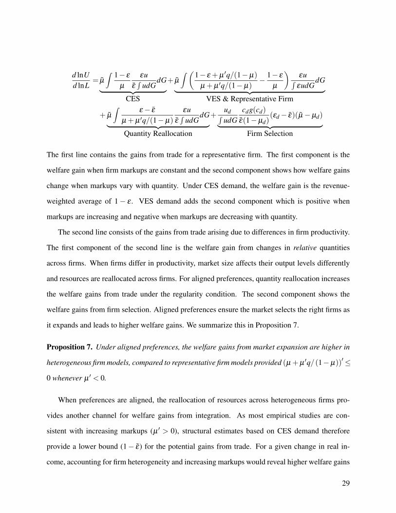
The first line contains the gains from trade for a representative firm. The first component is the

welfare gain when firm markups are constant and the second component shows how welfare gains

change when markups vary with quantity. Under CES demand, the welfare gain is the revenue-

weighted average of 1− ε . VES demand adds the second component which is positive when

markups are increasing and negative when markups are decreasing with quantity.

The second line consists of the gains from trade arising due to differences in firm productivity.

The first component of the second line is the welfare gain from changes in relative quantities

across firms. When firms differ in productivity, market size affects their output levels differently

and resources are reallocated across firms. For aligned preferences, quantity reallocation increases

the welfare gains from trade under the regularity condition. The second component shows the

welfare gains from firm selection. Aligned preferences ensure the market selects the right firms as

it expands and leads to higher welfare gains. We summarize this in Proposition 7.

Proposition 7. Under aligned preferences, the welfare gains from market expansion are higher in

heterogeneous firm models, compared to representative firm models provided (µ +µ ′q/(1−µ))′≤

0 whenever µ ′ < 0.

When preferences are aligned, the reallocation of resources across heterogeneous firms pro-

vides another channel for welfare gains from integration. As most empirical studies are con-

sistent with increasing markups (µ ′ > 0), structural estimates based on CES demand therefore

provide a lower bound (1− ε) for the potential gains from trade. For a given change in real in-

come, accounting for firm heterogeneity and increasing markups would reveal higher welfare gains

29

from trade. The magnitude of these additional gains depends on the markup variation (through

ε(q(c))− ε(q(cd)) and µ ′(q(c))) and on the productivity distribution (through g(cd)).

6 Conclusion

This paper examines the efficiency of market allocations when firms vary in productivity and

markups. Considering the Spence-Dixit-Stiglitz framework, the efficiency of CES demand is valid

even with productivity differences across firms. This is because market outcomes maximize rev-

enue, and under CES demand, private and social incentives are perfectly aligned.

Generalizing to variable elasticities of substitution, firms differ in market power which affects

the trade-off between quantity, variety and productivity. Unlike symmetric firm models, the mar-

ket distortions depend on the elasticity of demand and the elasticity of utility. Under CES demand,

these two elasticities are constant and miss out on meaningful trade-offs. When these elasticities

vary, the pattern of misallocations depends on how demand elasticities change with quantities, so

policy analysis should ascertain these elasticities and take this information into account. While

the modeling framework we consider provides a theoretical starting point to understand distortions

across firms, enriching the model with market-specific features can yield better policy insights.

Neary and Mrazova (2013) and Parenti, Ushchev, and Thisse (2017) provide further generaliza-

tions of demand and costs, and Bilbiie, Ghironi, and Melitz (2006) and Opp, Parlour, and Walden

(2013) consider dynamic misallocations. Future work can also provide guidance on the design of

implementable policies to realize further welfare gains.

We focus on international integration as a key policy tool to realize potential gains. Market

expansion does not guarantee welfare gains under imperfect competition. As Dixit and Norman

(1988) put it, this may seem like a “sad note” on which to end. But we find that integration

provides welfare gains when the two demand-side elasticities ensure private and social incentives

are aligned. The welfare gains from integration are higher than those obtained in representative

firm models with constant elasticities, because market expansion also leads to a better reallocation

30

of resources across heterogeneous firms. Further work might quantify the scope of integration as a

tool to improve the performance of imperfectly competitive markets.

31

A Appendix: Proofs

A.1 A Folk Theorem

In this context, we need to define the policy space. Provided Me and q(c), and assuming withoutloss of generality that all of q(c) is consumed, allocations are determined. The only questionremaining is what class of q(c) the policymaker is allowed to choose from. A sufficiently rich classfor our purposes is q(c), which are positive and continuously differentiable on some closed intervaland zero otherwise. This follows from the basic principle that a policymaker will utilize lowcost firms before higher cost firms. Proposition 1 shows without loss of generality that quantitiesproduced at the market equilibrium are continuously differentiable. So we restrict q to be in setsof the form

Q[0,cd ] ≡ {q ∈ C 1,> 0 on [0,cd] and 0 otherwise}.

We use the following shorthand throughout the proofs: G(x)≡∫ x

0 g(c)dc, R(x)≡∫ x

0 cρ/(ρ−1)g(c)dc.Proof of Proposition 1. Our assumptions imply the existence of a unique market equilibrium,which guarantees that R(c) is finite for admissible c. First note that at both the market equilibriumand the social optimum, L/Me = fe + f G(cd) implies utility of zero, so in both cases L/Me >

fe + f G(cd). The policymaker’s problem is

max MeL∫ cd

0q(c)ρg(c)dc subject to fe + f G(cd)+L

∫ cd

0cq(c)g(c)dc = L/Me

where the maximum is taken over choices of Me, cd, q∈Q[0,cd ]. We will exhibit a globally optimalq∗(c) for each fixed (Me,cd) pair, reducing the policymaker’s problem to a choice of Me and cd .We then solve for Me as a function of cd and finally solve for cd .Finding q∗(c) for Me,cd fixed. For convenience, define the functionals V (q),H(q) by

V (q)≡ L∫ cd

0v(c,q(c))dc, H(q)≡ L

∫ cd

0h(c,q(c))dc

where h(c,x)≡ xcg(c) and v(c,x)≡ xρg(c). One may show that V (q)−λH(q) is strictly concave∀λ .19 Now for fixed (Me,cd), consider the problem of finding q∗ given by

maxq∈Q[0,cd ]

V (q) subject to H(q) = L/Me− fe− f G(cd). (2)

Following Troutman (1996), if some q∗ maximizes V (q)−λH(q) on Q[0,cd ] for some λ and satis-

19Since h is linear in x, H is linear and since v is strictly concave in x (using ρ < 1) so is V .

32

fies the constraint then it is a solution to Equation (2). For any λ , a sufficient condition for someq∗ to be a global maximum of Q[0,cd ] is

D2v(c,q∗(c)) = λD2h(c,q∗(c)). (3)

This follows because (3) implies for any such q∗, ∀ξ s.t. q∗+ ξ ∈Q[0,cd ] we have δV (q∗;ξ ) =

λδH(q∗;ξ ) (where δ denotes the Gateaux derivative in the direction of ξ ) and q∗ is a global maxsince V (q)−λH(q) is strictly concave. Condition (3) is ρq∗(c)ρ−1g(c) = λcg(c), which impliesq∗(c) = (λc/ρ)1/(ρ−1).20 From above, this q∗ serves as a solution to maxV (q) provided thatH(q∗) = L/Me− fe− f G(cd). This will be satisfied by an appropriate λ since for fixed λ we have

H(q∗) = L∫ cd

0(λc/ρ)1/(ρ−1)cg(c)dc = L(λ/ρ)1/(ρ−1)R(cd)

so choosing λ as λ ∗ ≡ ρ (L/Me− fe− f G(cd))ρ−1 /Lρ−1R(cd)

ρ−1 makes q∗ a solution. In sum-mary, for each (Me,cd) a globally optimal q∗ satisfying the resource constraint is

q∗(c) = c1/(ρ−1) (L/Me− fe− f G(cd))/LR(cd) (4)

which must be > 0 since L/Me− fe− f G(cd) must be > 0 as discussed at the beginning.Finding Me for cd fixed. We may therefore consider maximizing W (Me,cd) where

W (Me,cd)≡MeL∫ cd

0q∗(c)ρg(c)dc = MeL1−ρ [L/Me− fe− f G(cd)]

ρR(cd)1−ρ . (5)

Direct investigation yields a unique solution to the FOC of M∗e (cd) = (1−ρ)L/( fe + f G(cd)) andd2W/d2Me < 0 so this solution maximizes W .Finding cd . Finally, we have maximal welfare for each fixed cd from Equation (5), explicitlyW (cd) ≡W (M∗e (cd),cd). We may rule out cd = 0 as an optimum since this yields zero utility.Solving this expression and taking logs shows that

lnW (cd) = lnρρ(1−ρ)1−ρL2−ρ +(1−ρ) [lnR(cd)− ln( fe + f G(cd))] .

Defining B(cd)≡ lnR(cd)− ln( fe + f G(cd)) we see that to maximize lnW (cd) we need maximizeonly B(cd). In order to evaluate critical points of B, note that differentiating B and rearranging

20By abuse of notation we allow q∗ to be ∞ at c = 0 since reformulation of the problem omitting this single pointmakes no difference to allocations or utility which are all eventually integrated.

33

using R′(cd) = cρ/(ρ−1)d g(cd) yields

B′(cd) ={

cρ/(ρ−1)d −R(cd) f/ [ fe + f G(cd)]

}/g(cd)R(cd). (6)

Since limcd−→0 cρ/(ρ−1)d = ∞ and limcd−→∞ cρ/(ρ−1)

d = 0 while R(cd) and G(cd) are bounded, thereis a positive interval [a,b] outside of which B′(x) > 0 for x ≤ a and B′(x) < 0 for x ≥ b. Clearlysupx∈(0,a]B(x),supx∈[b,∞)B(x) < supx∈[a,b]B(x) and therefore any global maximum of B occurs in(a,b). Since B is continuously differentiable, a maximum exists in [a,b] and all maxima occur atcritical points of B. From Equation (6), B′(cd) = 0 iff R(cd)/cρ/(ρ−1)

d −G(cd) = fe/ f . For cd thatsatisfy B′(cd) = 0, M∗e and q∗ are determined and inspection shows the entire system correspondsto the market allocation. Therefore B has a unique critical point, which is a global maximum thatmaximizes welfare.

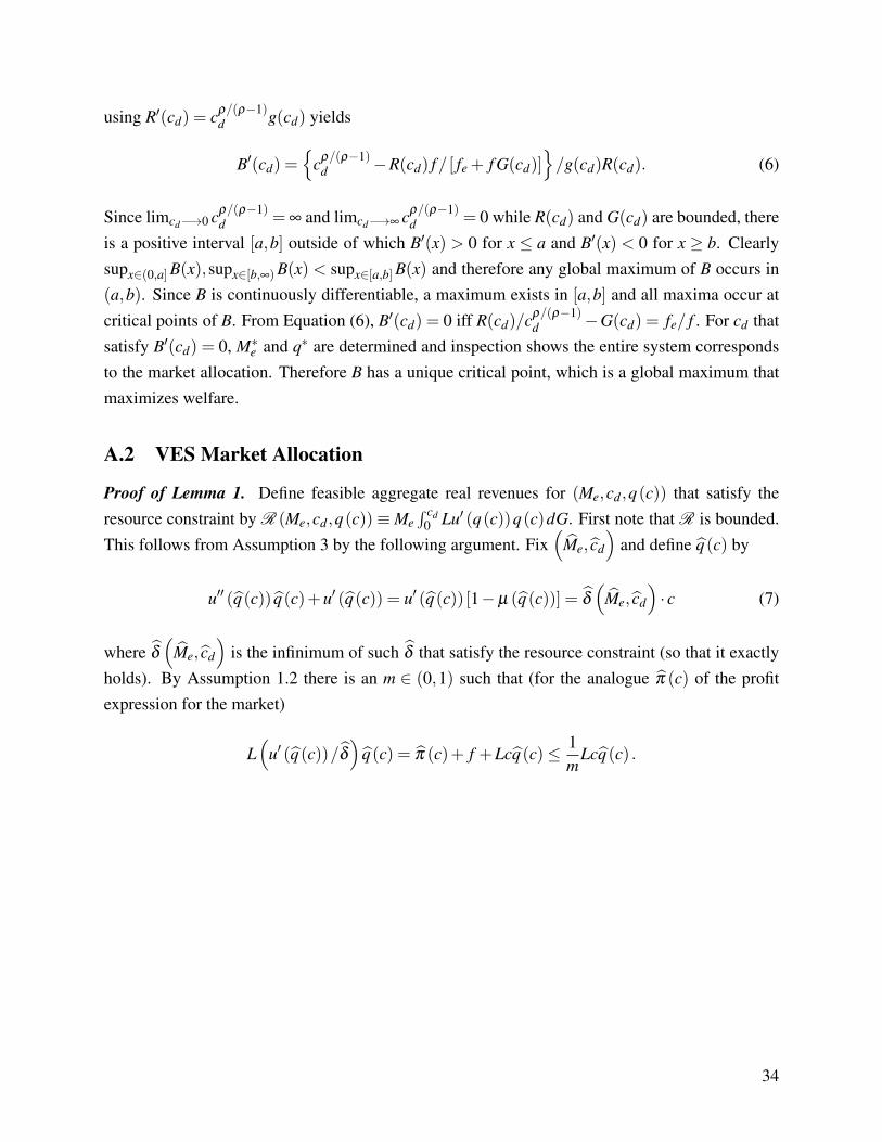
A.2 VES Market Allocation

Proof of Lemma 1. Define feasible aggregate real revenues for (Me,cd,q(c)) that satisfy theresource constraint by R (Me,cd,q(c))≡Me

∫ cd0 Lu′ (q(c))q(c)dG. First note that R is bounded.

This follows from Assumption 3 by the following argument. Fix(

Me, cd

)and define q(c) by

u′′ (q(c)) q(c)+u′ (q(c)) = u′ (q(c)) [1−µ (q(c))] = δ

(Me, cd

)· c (7)

where δ

(Me, cd

)is the infinimum of such δ that satisfy the resource constraint (so that it exactly

holds). By Assumption 1.2 there is an m ∈ (0,1) such that (for the analogue π (c) of the profitexpression for the market)

L(

u′ (q(c))/δ

)q(c) = π (c)+ f +Lcq(c)≤ 1

mLcq(c) .

34

Therefore aggregate real revenues at q(c) are bounded as:

R(

Me, cd, q(c))= δMe

∫ cd

0L(

u′ (q(c))/δ

)q(c)dG

≤ δMe

m

∫ cd

0Lcq(c)dG

= δMe

m

∫ cd

0Lc(u′)−1

(δc

1−µ (q(c))

)dG

≤ δ

mL2

fe

∫∞

0c(u′)−1

(δc

1−m

)dG

=1−m

mL2

fe

∫∞

0c(u′)−1

(c)dG (8)

where the second to last line follows from Assumption 1.2 and Me ≤ L/ fe (from the resourceconstraint), while the last by a change of variable in the integrand. Assumption 3.2 implies the lastline, 8, is finite.

We will now show that R(

Me, cd, ·)

is bounded for quantity distributions that satisfy the re-

source constraint. Let q(c) satisfy the resource constraint at(

Me, cd

), so that since

∫ cd0 Lcq(c)dG<

∞, it follows that G({c : cq(c) = ∞}) = 0. Since G is absolutely continuous, G({c : c = 0}) =0 and therefore G({c : q(c) = ∞}) ≤ G({c : cq(c) = ∞}) + G({c : c = 0}) = 0, i.e. q(c) isbounded almost everywhere and similarly q(c). Thus, for almost every c, there is a γ (c) ∈ [0,1]such that for qξ (c)≡ ξ q(c)+(1−ξ ) q(c), by the mean value theorem

u′ (q(c))q(c)−u′ (q(c)) q(c) = u′(qγ(c)

)(1−µ

(qγ(c)

))(q(c)− q(c)) .

35

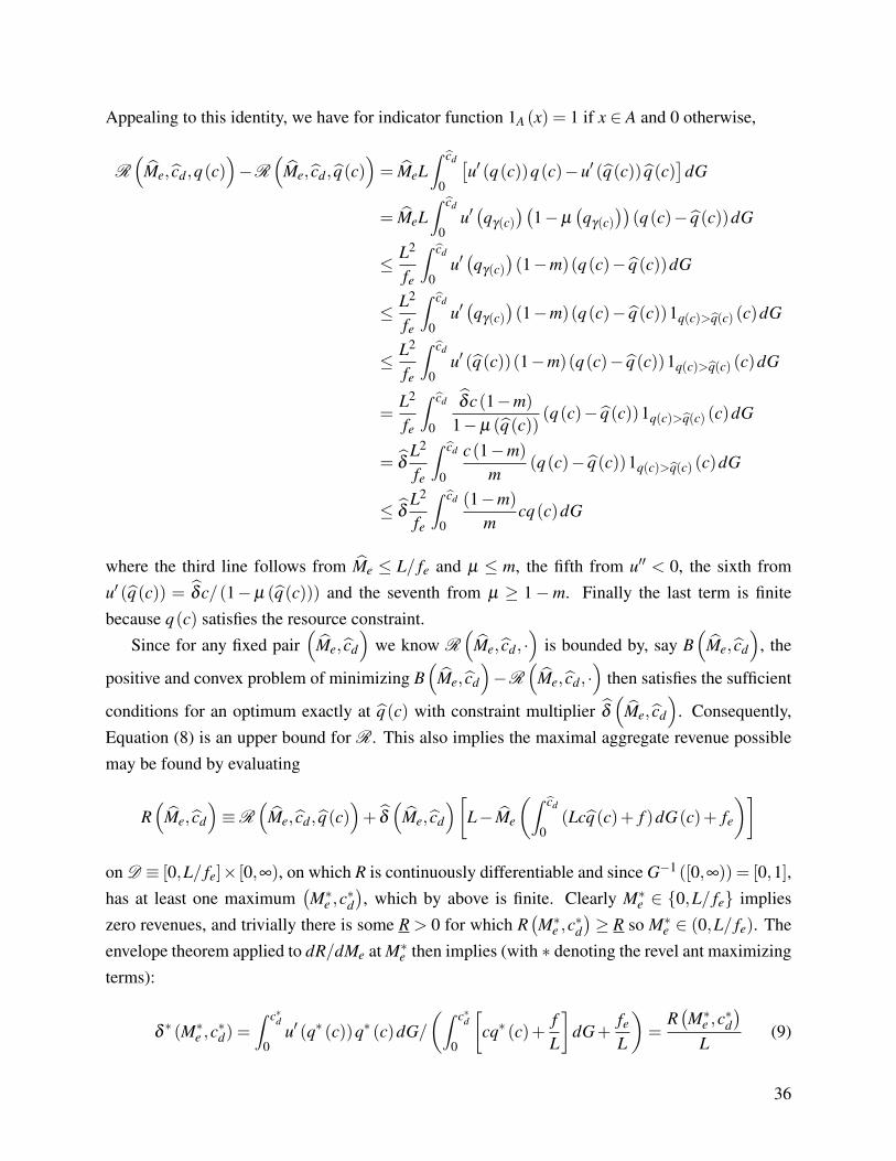
Appealing to this identity, we have for indicator function 1A (x) = 1 if x ∈ A and 0 otherwise,

R(

Me, cd,q(c))−R

(Me, cd, q(c)

)= MeL

∫ cd

0

[u′ (q(c))q(c)−u′ (q(c)) q(c)

]dG

= MeL∫ cd

0u′(qγ(c)

)(1−µ

(qγ(c)

))(q(c)− q(c))dG

≤ L2

fe

∫ cd

0u′(qγ(c)

)(1−m)(q(c)− q(c))dG

≤ L2

fe

∫ cd

0u′(qγ(c)

)(1−m)(q(c)− q(c))1q(c)>q(c) (c)dG

≤ L2

fe

∫ cd

0u′ (q(c))(1−m)(q(c)− q(c))1q(c)>q(c) (c)dG

=L2

fe

∫ cd

0

δc(1−m)

1−µ (q(c))(q(c)− q(c))1q(c)>q(c) (c)dG

= δL2

fe

∫ cd

0

c(1−m)

m(q(c)− q(c))1q(c)>q(c) (c)dG

≤ δL2

fe

∫ cd

0

(1−m)

mcq(c)dG

where the third line follows from Me ≤ L/ fe and µ ≤ m, the fifth from u′′ < 0, the sixth fromu′ (q(c)) = δc/(1−µ (q(c))) and the seventh from µ ≥ 1−m. Finally the last term is finitebecause q(c) satisfies the resource constraint.

Since for any fixed pair(

Me, cd

)we know R

(Me, cd, ·

)is bounded by, say B

(Me, cd

), the

positive and convex problem of minimizing B(

Me, cd

)−R

(Me, cd, ·

)then satisfies the sufficient

conditions for an optimum exactly at q(c) with constraint multiplier δ

(Me, cd

). Consequently,

Equation (8) is an upper bound for R. This also implies the maximal aggregate revenue possiblemay be found by evaluating

R(

Me, cd

)≡R

(Me, cd, q(c)

)+ δ

(Me, cd

)[L− Me

(∫ cd

0(Lcq(c)+ f )dG(c)+ fe

)]on D ≡ [0,L/ fe]× [0,∞), on which R is continuously differentiable and since G−1 ([0,∞)) = [0,1],has at least one maximum

(M∗e ,c

∗d

), which by above is finite. Clearly M∗e ∈ {0,L/ fe} implies

zero revenues, and trivially there is some R > 0 for which R(M∗e ,c

∗d

)≥ R so M∗e ∈ (0,L/ fe). The

envelope theorem applied to dR/dMe at M∗e then implies (with ∗ denoting the revel ant maximizingterms):

δ∗ (M∗e ,c

∗d) =

∫ c∗d

0u′ (q∗ (c))q∗ (c)dG/

(∫ c∗d

0

[cq∗ (c)+

fL

]dG+

fe

L

)=

R(M∗e ,c

∗d

)L

(9)

36

and thus δ ∗ ≥ R/L. Now consider that c∗d = 0 implies zero revenues so c∗d > 0 and at any positive,finite cd:

dR/dcd = MeL[u′ (q(cd)) q(cd)− δ (cd q(cd)+ f/L)

]= MeLδ

[µ (cd)

1−µ (cd)cd q(cd)− f/L

].

It follows that if cd q(cd)< m/(1−m) · f/L, then dR/dcd < 0. In particular,

cd q(cd) = u′ (q(cd)) q(cd)(1−µ (q(cd)))/δ ≤ u′ (q(cd)) q(cd)(1−m)/(R/L) . (10)

Since δ is increasing in cd (from the resource constraint), δ cd is increasing in cd and goes to infinityas cd does, which implies q(cd) goes to zero as cd goes to infinity. Since limq−→0 u′ (q)q = 0, thisimplies cd q(cd) −→ 0 as cd −→ 0 through Equation (10). Therefore for all sufficiently large cd ,dR/dcd < 0 so it must be that c∗d is finite. By the envelope theorem, at c∗d , it must be that

u′ (q∗ (c∗d))q∗ (c∗d) = δ∗ (c∗dq∗ (c∗d)+ f/L) . (11)

Now consider the equations that uniquely fix (Me,cd,q(c)) in the market allocation, namely:

u′ (q(cd))q(cd)/(cdq(cd)+ f/L) = δ ,∫ cd

0u′ (q(c))q(c)dG/

(∫ cd

0[cq(c)+ f/L]dG+ fe/L

)= δ ,

u′′ (q(c))q(c)+u′ (q(c)) = δc,

Me

(∫ cd

0Lcq(c)+ f dG+ fe

)= L.

The first line is Equation (11), while the second is Equation (9), the third is Equation (7) and thefourth holds from the definition of δ ∗. Since these conditions completely characterize every marketequilibrium, the uniqueness of the market equilibrium guarantees a unique solution here as well.

A.3 Static Distortion Results

Proof of Proposition 4. The result relies on the following relationship we first prove:

σ ≡ supc≤cmkt

d

ε

(qmkt(c)

)> δ/λ> inf

c≤coptd

ε(qopt(c)

)≡ σ . (12)

37

To see this recall δ = Mmkte∫ cmkt

d0 u′

(qmkt(c)

)qmkt(c)dG so σ > δ/λ because

δ/σ = Mmkte

∫ cmktd

0

(ε

(qmkt(c)

)/σ

)u(

qmkt(c))

dG < Mmkte

∫ cmktd

0u(

qmkt(c))

dG (13)

and λ is the maximum welfare per capita so λ > Mmkte∫ cmkt

d0 u

(qmkt(c)

)dG > δ/σ . A similar

argument shows λσ < δ , giving Equation (12). Now note that[u′′(

qmkt(c))

qmkt(c)+u′(

qmkt(c))]

/δ = c, u′(qopt(c)

)/λ = c. (14)

And it follows from Equations (14) we have[1−µ

(qmkt(c)

)]·u′(

qmkt(c))/u′(qopt(c)

)= δ/λ . (15)

When µ ′ and ε ′ have different signs, and since infq ε (q) > 0, from above in both cases it holdsthat infq>0 1−µ (q) = infq>0 ε (q) and supq>0 1−µ (q) = supq>0 ε (q). The arguments above haveshown that supq>0ε (q)> δ/λ > infq>0 ε (q) and therefore

supq>01−µ (q)> δ/λ > infq>01−µ (q) .

It follows from Equation (15) that for some c∗, 1−µ(qmkt(c∗)

)= δ/λ and therefore u′

(qmkt(c∗)

)=

u′ (qopt(c∗)) so qmkt(c∗) = qopt(c∗). Furthermore, qmkt(c) is strictly decreasing in c so with µ ′ 6= 0,c∗ is unique. Returning to Equation (15), using the fact that qmkt(c) is strictly decreasing in c alsoshows the relative magnitudes of qmkt(c) and qopt(c) for c 6= c∗.

Proof of Proposition 5. For α ∈ [0,1], define vα(q) ≡ αu′ (q)q+(1−α)u(q) and also definew(q)≡ u′ (q)q−u(q) so vα (q) = u(q)+αw(q). Consider the continuum of maximization prob-lems (indexed by α) defined as:

maxMe,cd ,q(c)

LMe

∫ cd

0vα (q(c))dG subject to L≥Me

(∫ cd

0Lcq(c)+ f dG+ fe

). (16)

Let the Lagrange multiplier associated with each α in Equation (16) be written as β (α). By ap-pealing to the envelope theorem and differentiating (16) in Me we have β (α) =Me

∫ cd0 vα (q(c))dG

and that dβ/dα = Me∫ cd

0 w(q(c))dG = Me∫ cd

0 u(q(c)) [ε(q)−1]dG < 0. The conditions charac-terizing the solution to every optimum also imply

β (α) = vα (q(cd))/(cdq(cd)+ f/L) ,

38

whereby we arrive at

dvα (q(cd))/dα = (dβ/dα)(vα (q(cd))/β )+β ((dcd/dα)q(cd)+ cd (dq(cd)/dα))

= w(q(cd))+ v′α (q(cd))(dq(cd)/dα)

= w(q(cd))+βcd (dq(cd)/dα)

so cancellation and rearrangement, using the expressions for β , dβ/dα above shows

βq(cd)(dcd/dα) = w(q(cd))− (vα (q(cd))/β )(dβ/dα)

= w(q(cd))−(

vα (q(cd))/Me

∫ cd

0vα (q(c))dG

)·Me

∫ cd

0w(q(c))dG.

We conclude that dcd/dα ≷ 0 when w(q(cd))∫ cd

0 vα (q(c))dG ≷ vα (q(cd))∫ cd

0 w(q(c))dG. Ex-panding this inequality we have (suppressing q(c) terms in integrands):

w(q(cd))∫ cd

0udG+αw(q(cd))

∫ cd

0wdG ≷ u(q(cd))

∫ cd

0wdG+αw(q(cd))

∫ cd

0wdG.

Cancellation and expansion again show this is equivalent to

u′ (q(cd))q(cd)∫ cd

0udG ≷ u(q(cd))

∫ cd

0u′q(c)dG.

Finally, this expression can be rewritten ε (q(cd)) ≷∫ cd

0 ε (q(c))u(q(c))dG/∫ cd

0 u(q(c))dG andsince q(c) is strictly decreasing in c, we see dcd/dα ≷ 0 when ε ′ ≶ 0. Note that Equation (16)shows α = 0 corresponds to the social optimum while α = 1 corresponds to the market equilib-rium. It follows that when ε ′ < 0 that dcd/dα > 0 so we have cmkt

d > coptd and vice versa for ε ′ > 0.

A.4 Welfare Gains from Trade

The sufficient condition for gains from trade follows from differentiating U = Me∫

u(q)dG = δ/ε

where the average elasticity of utility is ε ≡∫

εudG/∫

udG. An increase in market size raises themarginal utility of income at the rate of average markups d lnδ/d lnL =

∫µ pqdG/

∫pqdG ≡ µ .

From d lnδ/d lnL and d ln ε/d lnL, the change in welfare is

d lnUd lnL

= µ

[1+

∫ 1−µ− ε

µ +µ ′q/(1−µ)

εuε∫

udGdG]+

[ud∫udG

cdg(cd)

ε(1−µd)(εd− ε)(µ−µd)

].

39

When preferences are aligned, the second term in square brackets is positive because µ and (1−ε)

move in the same direction. The first term in square brackets is also positive when preferences arealigned, given the regularity condition that (µ +µ ′q/(1−µ))′ ≤ 0.Proof of Proposition 6. Following the discussion above, it is sufficient to show that for γ ≡ε (µ +µ ′q/(1−µ))−1,

1+∫ 1−µ− ε

µ +µ ′q/(1−µ)

εuε∫

udGdG =

∫ [1− ε +µ

′q/(1−µ)] γu

ε∫

udGdG≥ 0. (17)

This clearly holds for µ ′ ≥ 0, and for the other case where preferences are aligned, we have µ ′ <

0 < ε ′. Expanding Equation (17) for γ ≡∫

γ · (u/∫

udG)dG shows that∫ [1− ε +µ

′q/(1−µ)] γu

ε∫

udGdG =[1− ε−µ] γ/ε +1+

∫[µ−µ]

γuε∫

udGdG.

Since ε ′ > 0, 1− ε − µ > 0 and [1− ε−µ] γ/ε > 0. Therefore, it is sufficient to show that 1+∫[µ−µ] γu

ε∫

udGdG > 0. This sufficient condition is equivalent to

∫(µ + ε)

u∫udG

dG≥∫

µγu

γ∫

udGdG (18)

Since∫

γ · (u/γ∫

udG)dG = 1 and dµ/dc > 0, it follows that if dγ/dc < 0, then Equation (18)holds by stochastic dominance. As dγ/dc < 0 iff dγ/dq > 0, and ε ′ ≥ 0, it is sufficient thatµ +µ ′q/(1−µ) is decreasing in q , which is true by assumption.

40

ReferencesAlessandria, G. and H. Choi. 2007. “Do Sunk Costs of Exporting Matter for Net Export Dynam-

ics?” The Quarterly Journal of Economics 122 (1):289–336.

Arkolakis, C., A. Costinot, D. Donaldson, and A. Rodriguez-Clare. forthcoming. “The ElusivePro-Competitive Effects of Trade.” Review of Economic Studies .

Arkolakis, C., A. Costinot, and A. Rodriguez-Clare. 2012. “New trade models, same old gains?”American Economic Review 102 (1):94–130.

Arkolakis, Costas. 2010. “Market Penetration Costs and the New Consumers Margin in Interna-tional Trade.” Journal of Political Economy 118 (6):1151–1199.

Asplund, M. and V. Nocke. 2006. “Firm turnover in imperfectly competitive markets.” The Reviewof Economic Studies 73 (2).

Atkeson, A. and Burstein. 2010. “Innovation, Firm Dynamics, and international Trade.” Journalof Political Economy 118 (3):433–484.

Baldwin, R. E. and F. Robert-Nicoud. 2008. “Trade and growth with heterogeneous firms.” Journalof International Economics 74 (1):21–34.

Bartelsman, E. J. and M. Doms. 2000. “Understanding productivity: Lessons from longitudinalmicrodata.” Journal of Economic literature 38 (3).

Baumol, W. J. and D. F. Bradford. 1970. “Optimal Departures From Marginal Cost Pricing.” TheAmerican Economic Review 60 (3):265–283.

Benassy, J. P. 1996. “Taste for variety and optimum production patterns in monopolistic competi-tion.” Economics Letters 52 (1):41–47.

Bernard, A. B., J. Eaton, J. B. Jensen, and S. Kortum. 2003. “Plants and Productivity in Interna-tional Trade.” American Economic Review .

Bernard, A. B., J. B. Jensen, S. J. Redding, and P. K. Schott. 2007. “Firms in International Trade.”The Journal of Economic Perspectives 21 (3):105–130.

Bilbiie, F. O., F. Ghironi, and M. J. Melitz. 2006. “Monopoly power and endogenous variety indynamic stochastic general equilibrium: distortions and remedies.” manuscript, University ofOxford, Boston College, and Princeton University .

Bykadorov, Igor, Alexey Gorn, Sergey Kokovin, and Evgeny Zhelobodko. 2015. “Why are lossesfrom trade unlikely?” Economics Letters 129:35–38.

Campbell, J. R. and H. A. Hopenhayn. 2005. “Market Size Matters.” Journal of Industrial Eco-nomics 53 (1):1–25.

41

Costinot, Arnaud and Andrés Rodriguez-Clare. 2013. “Trade Theory with Numbers: Quantify-ing the Consequences of Globalization.” In In: Helpman, E.(Ed.), Handbook of internationaleconomics. Citeseer.

de Blas, B. and K. Russ. 2010. “Understanding Markups in the Open Economy under BertrandCompetition.” American Economic Journal: Macroeconomics 7:157–180.

De Loecker, Jan, Pinelopi K. Goldberg, Amit K. Khandelwal, and Nina Pavcnik. 2012. “Prices,markups and trade reform.” Tech. rep., National Bureau of Economic Research.

De Loecker, Jan and Frederic Warzynski. 2012. “Markups and Firm-Level Export Status.” TheAmerican Economic Review 102 (6):2437–2471.

Dhingra, Swati and John Morrow. 2016a. “Efficiency in Heterogeneous Firm Trade Models.”Working Paper .

———. 2016b. “Existence and Uniqueness of the Market Equilibrium in a VES Economy.” .

Dhyne, Emmanuel, Amil Petrin, and Frederic Warzynski. 2011. “Prices, Markups and Quality atthe Firm-Product Level.” Tech. rep., Mimeo, University of Minnesota.

Dixit, A. K. and V. Norman. 1988. Theory of international trade. Cambridge Univ. Press.

Dixit, A. K. and J. E. Stiglitz. 1977. “Monopolistic Competition and Optimum Product Diversity.”The American Economic Review 67 (3):297–308.

Eckel, Carsten. 2008. “Globalization and specialization.” Journal of International Economics75 (1):219–228. URL http://ideas.repec.org/a/eee/inecon/v75y2008i1p219-228.html.

Epifani, P. and G. Gancia. 2011. “Trade, markup heterogeneity and misallocations.” Journal ofInternational Economics 83 (1):1–13.

Feenstra, R. and H. L. Kee. 2008. “Export variety and country productivity: Estimating the monop-olistic competition model with endogenous productivity.” Journal of International Economics74 (2):500–518.

Feenstra, R. C. 2003. “A homothetic utility function for monopolistic competition models, withoutconstant price elasticity.” Economics Letters 78 (1):79–86.

———. 2006. “New Evidence on the Gains from Trade.” Review of World Economics 142 (4):617–641.

Foster, L., J. Haltiwanger, and C. Syverson. 2008. “Reallocation, firm turnover, and efficiency:Selection on productivity or profitability?” American Economic Review 98 (1):394–425.

Foster, L., J. C. Haltiwanger, and C. J. Krizan. 2001. “Aggregate productivity growth. Lessonsfrom microeconomic evidence.” In New developments in productivity analysis. University ofChicago Press.

42

Goldberg, P. and Michael Knetter. 1997. “Goods prices and exchange rates: what have we learned.”Journal of Economic Literature 5862.

Grossman, Gene M. and Elhanan Helpman. 1993. Innovation and Growth in the Global Economy.MIT Press.

Helpman, E., O. Itskhoki, and S. J. Redding. 2013. “Trade and Labor Market Outcomes.” Advancesin Economics and Econometrics 2:459–504.

Helpman, E. and P. R. Krugman. 1985. Market Structure and Foreign Trade: increasing returns,imperfect competition, and the international economy. MIT Press.

Holt, C. A. and S. K. Laury. 2002. “Risk aversion and incentive effects.” American EconomicReview 92 (5):1644–1655.

Katayama, H., S. Lu, and J. R. Tybout. 2009. “Firm-level productivity studies: illusions and asolution.” International Journal of Industrial Organization 27 (3):403–413.

Klette, Tor J. 1999. “Market power, scale economies and productivity: estimates from a panel ofestablishment data.” The Journal of Industrial Economics 47 (4):451–476.

Krugman, P. 1979. “Increasing Returns, Monopolistic Competition, and International Trade.”Journal of International Economics 9 (4):469–479.

Krugman, P. R. 1987. “Is free trade passé?” The Journal of Economic Perspectives 1 (2).

Krugman, Paul R. 1980. “Scale Economies, Product Differentiation, and the Pattern of Trade.”American Economic Review 70 (5):950–959.

Mankiw, N. G. and M. D. Whinston. 1986. “Free entry and social inefficiency.” The RAND Journalof Economics :48–58.

Matsuyama, Kiminori. 1995. “Complementarities and Cumulative Processes in Models of Monop-olistic Competition.” Journal of Economic Literature 33 (2):701–729. URL http://ideas.repec.org/a/aea/jeclit/v33y1995i2p701-729.html.

Melitz, M. J. and S. J. Redding. 2012. “Heterogeneous Firms and Trade.” Handbook of Interna-tional Trade (commissioned) .

Melitz, Marc and Daniel Trefler. 2012. “Gains from Trade when Firms Matter.” Journal of Eco-nomic Perspectives 26.

Melitz, Marc J. 2003. “The Impact of Trade on Intra-Industry Reallocations and Aggregate Indus-try Productivity.” Econometrica 71 (6):1695–1725.

Melitz, Marc J. and Gianmarco I. P. Ottaviano. 2008. “Market Size, Trade, and Productivity.”Review of Economic Studies 75 (1):295–316.

Melitz, Marc J. and Stephen J. Redding. 2013. “Firm Heterogeneity and Aggregate Welfare.” Tech.rep., National Bureau of Economic Research.

43

Melvin and R. D. Warne. 1973. “Monopoly and the theory of international trade.” Journal ofInternational Economics 3 (2):117–134.

Neary, J. Peter and Monika Mrazova. 2013. “Not so demanding: Preference structure, firm behav-ior, and welfare.” Tech. rep., University of Oxford, Department of Economics.

Nocco, Antonella, Gianmarco I. P. Ottaviano, and Matteo Salto. 2013. “Monopolistic Competitionand Optimum Product Selection: Why and How Heterogeneity Matters.” CEP Discussion Paper1206.

Opp, Marcus M., Christine A. Parlour, and Johan Walden. 2013. “A Theory of Dynamic ResourceMisallocation and Amplification.” Available at SSRN 2049447 .

Parenti, Mathieu, Philip Ushchev, and Jacques-François Thisse. 2017. “Toward a theory of mo-nopolistic competition.” Journal of Economic Theory 167:86–115.

Pavcnik, N. 2002. “Trade Liberalization, Exit, and Productivity Improvements: Evidence fromChilean Plants.” The Review of Economic Studies 69 (1):245–276.

Post, T., M. J. Van den Assem, G. Baltussen, and R. H. Thaler. 2008. “Deal or no deal? Decisionmaking under risk in a large-payoff game show.” The American Economic Review 98 (1):38–71.

Roberts, Mark J. and Dylan Supina. 1996. “Output price, markups, and producer size.” EuropeanEconomic Review 40 (3):909–921.

———. 2001. “Output price and markup dispersion in micro data: The roles of producer hetero-geneity and noise.” Advances in Applied Microeconomics 9:1–36.

Saha, A. 1993. “Expo-power utility: A’flexible’form for absolute and relative risk aversion.” Amer-ican Journal of Agricultural Economics :905–913.

Spence, M. 1976. “Product Selection, Fixed Costs, and Monopolistic Competition.” The Reviewof Economic Studies 43 (2):217–235.

Stiglitz, J. E. 1986. “Towards a more general theory of monopolistic competition.” Prices, compe-tition and equilibrium :22.

Syverson, C. 2004. “Market Structure and Productivity: A Concrete Example.” Journal of PoliticalEconomy 112 (6):1181–1222.

———. 2011. “What Determines Productivity?” Journal of Economic Literature 49 (2).

Troutman, J. L. 1996. Variational calculus and optimal control: Optimization with elementaryconvexity. New York: Springer-Verlag.

Tybout, J. R. 2003. “Plant-and firm-level evidence on "new" trade theories.” Handbook of Inter-national Trade 1:388–415.

Venables, A. J. 1985. “Trade and trade policy with imperfect competition: The case of identicalproducts and free entry.” Journal of International Economics 19 (1-2):1–19.

44

Vives, X. 2001. Oligopoly pricing: old ideas and new tools. The MIT press.

Weyl, E. G. and M. Fabinger. 2012. “Pass-through as an Economic Tool.” University of Chicago,mimeo .

Zhelobodko, Evgeny, Sergey Kokovin, Mathieu Parenti, and Jacques-François Thisse. 2012.“Monopolistic competition: Beyond the constant elasticity of substitution.” Econometrica80 (6):2765–2784.

45

Tables

Table 1: Private and Social Markups for Common Utility Forms(1− ε)′ ,µ ′ < 0 (1− ε)′ ,µ ′ > 0

HARA (α < 0): (q/(1−ρ)+α)ρ−αρ

ρ/(1−ρ) HARA (α > 0): (q/(1−ρ)+α)ρ−αρ

ρ/(1−ρ)

Expo-power (α < 0):1−exp(−αq1−ρ)

αExpo-power (α > 0):

1−exp(−αq1−ρ)α

CARA, Quadratic

46

Table 2: Distortions for Aligned Preferences by Demand ElasticitiesIncreasing Markups Decreasing Markups

µ ′,(1− ε)′ > 0 µ ′,(1− ε)′ < 0Quantities High-Cost Skewed: Quantities Low-Cost Skewed:qmkt(c)< qopt(c) for c < c∗ qmkt(c)> qopt(c) for c < c∗

qmkt(c)> qopt(c) for c > c∗ qmkt(c)< qopt(c) for c > c∗

Productivity Too Low: cmktd > copt

d Productivity Too High: cmktd < copt

d

47

Figure Legends

Figure 1: Bias in Firm Production for Aligned Preferences with Increasing Markupsµ ′,(1− ε)′ > 0

48