Embed Size (px)
Citation preview

T H E I N T E R N A T I O N A L J O U R N A L O F
CONDITIONMONITORING
Volume 1 | Issue 1 | June 2011
OFFICIAL JOURNAL OF THE BRITISH INSTITUTE OF NON-DESTRUCTIVE TESTING

The International Journal of Condition Monitoring | Volume 1 | Issue 1 | June 20112
CONTENTS
Volume 1 | Issue 1 | June 2011
Comment ....................................................................... 3
Trends in industrial oil analysis – a review,by P O Vähäoja and H V S Pikkarainen ......................... 4
A comparison of methods for separation of deterministic and random signals,by R B Randall, N Sawalhi and M Coats .....................11
Condition monitoring of brushless DC motor-based electromechanical linear actuators using motor current signature analysis,by G Sreedhar Babu, A Lingamurthy and A S Sekhar ........................................................................20
A novel feature selection algorithm for high-dimensional condition monitoring data,by Kui Zhang, A D Ball, Yuhua Li and Fengshou Gu .....................................................................33
The International Journal of Condition Monitoring | Volume 1 | Issue 1 | June 20111
COMMENT
I am pleased to introduce this the first issue of The International Journal of Condition Monitoring (IJCM).
IJCM is a scientific-technical journal containing high-quality, innovative, in-depth peer-reviewed papers on all the condition monitoring disciplines, including prognostics and root cause analysis. IJCM will be published four times a year online. It will be of interest to all those concerned with condition monitoring and will contain material that is highly relevant to a wide range of readers, including academics, scientists and engineers.
The journal, together with the annual International Condition Monitoring Conference, organised by The British Institute of NDT in partnership with the Society for Machinery Failure Prevention Technology (USA), and the recently launched International Society for Condition Monitoring, create a powerful condition monitoring triangle at a high scientific-technical level. This triangle, which covers all areas of condition monitoring, is the result of joint efforts of the high-level international scientific-technical community associated with the annual International Condition Monitoring Conference. The community consists of academic and industry members from more than 30 countries worldwide, including representatives of renowned universities from all continents and leading industrial players: BAE Systems, Boeing, Rolls-Royce, Shell and others.
The launch of the journal demonstrates the international growth and value of innovative research and developments provided by the community. The creation and inauguration of this journal are solid evidence of the triangle members’ commitment to advancing the field of conditioning monitoring and making the benefits of this science available to the international community. The IJCM also demonstrates the field’s dedication to collaborative research and study that have produced outstanding results, benefiting the industries and nations that we serve.
I would like to thank all members of the CM triangle for their great efforts in creating the IJCM.
The Condition Monitoring Conferences and the Society will strongly support the Journal, and I am sure that this will result in it soon becoming established as the leading publication in its field.
I am pleased to invite readers of the Journal to become active members of the CM triangle by submitting a paper to the journal (http://mc.manuscriptcentral.com/ijcm), and to the International Condition Monitoring Conference CM/MFPT 2012 (London, UK, 12-14 June 2012) and by applying for membership of the International Society for Condition Monitoring.
Please enjoy this issue…Thank you.
Professor Len GelmanHonorary Technical Editor, International Journal of Condition MonitoringChair in Vibro-Acoustical Monitoring, Cranfield UniversityChairman, the Condition Monitoring Technical Committee, BINDTDirector, International Institute of Acoustics and Vibration
Editorial BoardEditor: Mr D Gilbert (UK)Honorary Technical Editor: Prof L Gelman (UK)Vice Honorary Technical Editor: Dr N Martin (France)International Editorial Panel (regional editors): Prof S Heyns (South Africa) Prof A Hope (UK) Prof R Randall (Australia)
Editorial contributions should be addressed to The Editor, IJCM, BINDT, Newton Building, St George’s Avenue, Northampton NN2 6JB, UK. Tel: +44 (0)1604 89 3811; Fax: +44 (0)1604 89 3861; Email: [email protected]
Paper SubmissionThe British Institute of Non-Destructive Testing invites contributions of quality and originality which will interest the readership of IJCM. Technical papers submitted are peer-reviewed. Referees are appointed by the Institute’s Condition Monitoring Technical Committee, which directs the Journal. This Committee is supported by the Editorial Board.The decision to publish rests with the Condition Monitoring Technical Committee.Online submission at http://mc.manuscriptcentral.com/ijcmGuidelines for Authors are available on request.
CirculationJoan Paintin. Tel: +44 (0)1604 89 3811.
Subscriptions IJCM is free to members of The British Institute of Non-Destructive Testing. Members may access IJCM directly via the members’ log-in area of the www.bindt.org website without having to log in a second time on Atypon-Link.Non-members and institutions may take out subscriptions to IJCM at the following rate for 2011/2012: £66.50 (4 issues).
Copyright© 2011 The British Institute of Non-Destructive Testing.This publication is copyright under the Berne Convention and the International Copyright Convention. All rights reserved. Apart from any fair dealing for the purpose of private study, research, criticism or review, as permitted under the Copyright, Designs and Patents Act 1988, no part of this publication may be reproduced, stored in a retrieval system or transmitted in any form or by any means without the prior permission of the copyright owners. Reprographic reproduction is permitted only in accordance with the terms of licences issued by the Copyright Licensing Agency, 90 Tottenham Court Road, London W1P 9HE. Unlicensed multiple copying of the contents of the publication without permission is illegal.The views expressed in this publication are those of the authors and except where specifically indicated are not necessarily those of The British Institute of Non-Destructive Testing.ISSN 2047-6426Information on IJCM and other Institute services can be found on the World Wide Web at: http://www.bindt.orgPublished by The British Institute of Non-Destructive Testing, Newton Building, St George’s Avenue, Northampton NN2 6JB, UK . Tel: +44 (0)1604 89 3811; Fax: +44 (0)1604 89 3861; Email: [email protected] British Institute of Non-Destructive Testing is a Limited Company (Reg No 969051 England) and a Charity (Reg No 260666)).
Member of the Association of Learned and Professional Society Publishers
Members:Prof R Allen (UK) Prof J Antoni (France) Prof W Bartelmus (Poland) Dr C Byington (USA) Prof M Crocker (USA)Dr N Eklund (USA)Mr V Fox (USA) Prof T-H Gan (UK)Prof K Horoshenkov (UK)Prof P Irving (UK) Prof I Jennions (UK) Prof P John (UK)Dr E Juuso (Finland)Dr K Keller (USA)
Dr S King (UK)Dr R Klein (Israel)Prof V Kostyukov (Russia)Prof L Kuravsky (Russia)Prof T Lago (Sweden) Prof S Lahdelma (Finland)Prof A Lucifredi (Italy) Prof S Radkowski (Poland) Prof R Smid (Czech Republic)Prof J Strackeljan (Germany)Prof L Swedrowski (Poland)Prof P Trampus (Hungary)Prof J Vizintin (Slovenia) Dr L Wang (UK)Prof P White (UK)

The International Journal of Condition Monitoring | Volume 1 | Issue 1 | June 20114
FEATURE | OIL ANALYSIS
This article is a literature review of current trends in industrial oil analysis. The most significant off-line (laboratory) oil analysis techniques, ie wear metal analysis, solid debris analysis and additive analysis, are presented with some application remarks. Because more real-time data is continuously required in industry to support maintenance decisions, on- and in-line oil analysis techniques are especially concentrated on in the review of current literature. In particular solid debris and other contaminant analysers and oil condition sensors are discussed thoroughly. Certain commercial players in the industrial oil analysis field, such as lubricant manufacturers, oil analysis laboratories, machine manufacturers and measurement instrument manufacturers, are handled as well. A comparison of oil analysis techniques with vibration monitoring and acoustic emission is carried out.
1. IntroductionModern maintenance would ideally be based on the real condition of machines. Condition monitoring of machinery can be anything from simple visual inspection to continuously functioning real-time condition monitoring systems. Oil analysis is a significant part of condition-based maintenance, because oil tells about the history of the machine since the last oil change. Oil includes the wear metals and contaminants and, for example, may indicate the need to repair certain machine elements or inform about problems in oil filtration. Oil analysis also reveals the condition of the oil itself, whether its properties are still at a sufficiently good state or if an oil change will be required soon. Oil analysis may first be seen as a cost only, but one should notice that oil analysis may either directly or indirectly help to improve the availability and performance of the machines and improve the quality of the final products (for example in metal working). An efficient oil analysis programme is often based on off-line oil analysis, meaning thorough laboratory analyses of oil properties. However, there are more and more requirements for real-time oil analysis data to support the maintenance decisions. A lot of continuously measuring on-line/in-line oil analysis sensors are commercially available. However, these sensors often measure one property only, for instance particle size distribution or moisture. The amount of data these sensors produce may be vast, hence correct and reliable alarm and action limits should be chosen. Of course, if possible in a sensible time, unusual findings can be confirmed by laboratory analyses.
Trends in industrial oil analysis – a reviewP O Vähäoja and H V S Pikkarainen
Pekka O Vähäoja is with Winwind Oy, Kaarnatie 38, FI-90530 Oulu, Finland. Email: [email protected]
Harri V S Pikkarainen is with Kemi-Tornio University of Applied Sciences, Optical Measurement Laboratory, Kiveliönkatu 36, FI-94600 Kemi, Finland.
2. Off-line oil analysisOff-line oil analyses require oil sampling. The oil sample must be taken in the same way at the same place every time in order to make trending of the analysis results possible. Contamination of the samples has to be prevented during oil sampling and the samples should preferably be taken from a running machine under its normal operating conditions. If oil samples are not taken in the correct way, they will not be representative and can lead to totally the wrong conclusions about the status of the machine being studied. Efficiency of an oil analysis programme depends on the time schedule of sampling. Failures must be observed at the earliest possible stage to determine the optimal corrective action and its timetable(1-2).
2.1 Wear metal analysisWear metal analysis techniques are used to determine the total concentrations of wear, contaminant and additive metals (and also some half- and non-metal elements). With the help of this information, the need for machine repair, oil change or oil filtration can be decided upon and the possible operational time before machine stoppage or even the usable lifetime of the whole machine can be evaluated. The most used wear metal analysis methods are: atomic absorption spectrometry (flame and electrothermal AAS), optical emission spectrometry (inductively coupled plasma or rotating disk electrode OES), mass spectrometry (inductively coupled plasma MS), X-ray fluorescence spectrometry (XRF) and neutron activation analysis (NAA). Due to the complex and viscous nature of lubricating oils, they may require pre-treatment before wear metal analysis(3).
In AAS techniques, the atomisation source is either a flame (FAAS) or electrically-heated graphite tube (ETAAS). A hollow cathode lamp emits UV or visible light at the characteristic wavelength of the studied element, atoms of which in the sample absorb the radiation. The amount of absorption is proportional to the amount of studied element in the sample. The main problem of the AAS techniques is their sequential nature, ie concentrations of only one element in the sample can be determined at a time and determination of concentrations of the next element needs a new measurement (and often a change of the hollow cathode lamp) and so on. This means that determination of various elements is very time-consuming(1,4). The FAAS technique is suitable when certain indicator metals of wearing are detected(5) and it has been applied widely in wear metal analysis of oils for decades now(6-8). The ETAAS technique offers higher sensitivity, but the sensitivity of the FAAS technique is usually sufficient for condition monitoring purposes. Typical pre-treatment methods of oil samples with AAS techniques are dissolution with organic solvents, wet digestion with and without microwave-assistance, and emulsification.
Submitted 08.05.10 Accepted 04.08.10

The International Journal of Condition Monitoring | Volume 1 | Issue 1 | June 20115
OIL ANALYSIS | FEATURE
An inductively coupled plasma-optical emission spectrometer (ICP-OES) is a very widely used measurement technique in oil analysis. Atomisation, sometimes ionisation, and excitation of the elements of the sample are carried out by using plasma. Death of the excitation states cause element-specific emission spectra to be produced. ICP-OES makes simultaneous analysis of over 70 elements possible; its linear determination range is wide, chemical interferences are minimal and the detection limits are low. The drawbacks of this technique are spectral interferences, matrix effects in nebulisation and excitation stages, and the high purchase and operating costs(1,4). Similar pre-treatments of oil samples as with AAS techniques can be applied(5,7,9-11).
Atoms can also radiate specific emission lines in the X-ray region. This property is applied in X-ray fluorescence spectrometry (XRF), which can be used to detect both additive and wear metals in oils. Certain lighter elements, such as Mg, Si and Al, cannot be monitored due to X-ray absorption and scattering by the oil if they are suspended in oil. The method is non-destructive, measurements are fast, and accuracy and precision of the measurements are good. Sensitivity of the XRF is not very high and instruments may be relatively expensive(1,4). One benefit of the XRF is that no sample pre-treatment is required, but pre-treatment of oil samples may improve efficiency of the XRF(12-13).
2.2 Solid debris analysisMetallic solid debris in oils is due to different types of wearing phenomena of metallic machine elements. Non-metallic solid debris can originate, for example, from filters, seals or paints. Solid sludge containing carbon deposits is produced by severe oxidation of the oil. Internal combustion engine oils usually include large amounts of solid carbonaceous residues caused by the combustion process, also known as soot. Contamination with process chemicals or environmental dust also increases the amount of solid debris in oils. Patch analysis is one of the oldest and most efficient methods of off-line solid debris analysis. A known volume of lubricating oil is filtrated through a filter membrane with a suitable pore size. The pore size of 0.45 μm is used to determine the total amount of solid particles in the oil. The solid debris trapped on the membrane can be studied in different ways. One such way is manual particle counting by a microscope. It should be noted that different operators will get slightly different results and the results of manual counting also usually differ from the results determined by automatic particle counters. Manual particle counting can sometimes be the only choice with some oils. By usingmmicroscopic inspection (for example the use of an optical or scanning electron microscope), information about shapes, colours, edge profiles and textures of the particles, ie about their morphology, can be produced. This information is useful when there is a need to detect the source of the particles, their wearing mechanisms and the status of the machine(1-2). Ferrographic techniques can be roughly divided into two categories: direct reading ferrographs and devices of analytical ferrography. These are produced, for example, by Predict Inc(14). Other devices based on magnetism and detecting ferrous particles are commercially available, such as the much used PQ Quantifier developed by Analex Ltd(15).
The cleanliness of hydraulic fluids and other oil systems with close tolerances have been monitored by means of automatic particle counters for a long time(16). A collimated light beam is passed through the oil sample to the detector in optical particle counters. When a particle hits the light beam, it blocks an amount of light proportional to its size. The light blockage is detected as a change in electrical signal. Some optical sensors are based on light scattering from the particle and they are more sensitive, but their measurement range is narrower than in light blockage sensors. When the detector is calibrated against calibration standards, particle size and count data can be generated. Optical counters are influenced by fluid opacity, ie its darkness, air bubbles and water. Optical counters may also suffer from coincidence error if large amounts of small particles are present in the sample. This means that groups of various small particles are seen as single large particles that causes erroneous results. Typical optical laboratory counters are Pamas SBSS, HIAC ABS-2 or 8012 or Hydac ALPC 9000 series(1,17-19). Particle counters can also be based on flow decay, ie the use of mono-size micro sieves blocked by particles, or mesh obscuration, ie pressure differential principle. Flow decay particle counters utilise different types of microsieve such as with 5, 10 or 15 µm pore size, which can be selected to the specific test based on the viscosity of the oil studied. The flow decay counter can be effective as long as the calibration formula converting the flow decay data to ISO cleanliness codes is valid. Selection of the correct pore size of the microsieve can sometimes be problematic when unknown samples are measured. Mesh obscuration particle counters utilise three micro-screens with 2, 5 and 15 µm pore sizes. Particles retained on micro-screens cause pressure drops which are measured and the pressure data is converted to particle count data and further to ISO cleanliness codes. Careful calibration of the counters with the known standard material is needed, but the mesh obscuration counters are effective for most oils, independent of their colour, and they are not usually sensitive to entrained air or water(1).
Fluid Imaging Inc has developed a particle image analysis method called the FlowCAM. It can be used in continuously imaging mode or in fluorescence triggered mode. A computer analyses the imaged particles by calculating length, width, equivalent spherical diameter, area and aspect ratio. In addition to laboratory measurements, determinations in situ can also be achieved. The FlowCAM has a wide measurement range (particle sizes of 1 µm - 3 mm) and a very high depth of focus. Interesting features can be calculated in real-time and later the images can be processed in desired ways(20). LaserNet Fines by SpectroInc is a system with applications for off-line, but also for in-/on-line, monitoring of wear debris in oils. It is capable of carrying out morphological analysis of wear particles. The system determines size distributions and shape characteristics of solid debris in oils in the size range of 5-100 µm. The device is based on parallel/series CCD technology, high-speed image processing and neural net classification. Particles larger than 20 µm are automatically classified to six different classes: cutting, severe sliding, fatigue, non-metals, fibres and water droplets. The total free water amount can also be calculated. Because the optical system of the LaserNet Fines uses transmitted light, particle colours, textures and surface attributes cannot be determined. The most recent version of

The International Journal of Condition Monitoring | Volume 1 | Issue 1 | June 20116
FEATURE | OIL ANALYSIS
the LaserNet Fines off-line device, ie Spectro LNF Q200, is also capable of determining the dynamic viscosity of the fluid(21-22).
2.3 Additive analysisLubricating oils typically consist of a base oil and different additives for improving certain properties of the base oil, producing totally new properties or weakening certain unwanted properties or preventing harmful reactions. The total amounts of the main elements in certain additives can be determined by means of the earlier presented atomic spectroscopic methods. Other additive analysis methods are infrared spectroscopy (IR), chromatographic techniques, nuclear magnetic resonance spectroscopy (NMR) and mass spectroscopy (MS)(1).
Infrared spectroscopy is based on the absorption of infrared radiation by molecules of the sample. IR produces information about functional groups of molecules without destructing the sample. IR can be used either for qualitative or quantitative analysis. Examples of quantitative measurements of oils using IR are shown in the literature(23-24). In addition to determining different additives, IR can be used to identify different oil types(25). Oil oxidation, sulphation, nitration or water contamination can also be monitored by means of the IR techniques(26-28). Oil samples must not necessarily be pre-treated prior to IR measurement, but usually dilution with a suitable solvent is needed.
2.4 Commercial off-line oil analysis suppliersLubricant manufacturers have oil analysis programs for the lubricants they sell. Typical programs are, for example, Shell LubeAnalyst or ExxonMobil Signum. The basic analysis packages may include the following: appearance, viscosity, water content, wear metals, particle count, oxidation and TAN. It is usually also possible to order more detailed analysis packages(29-30). Statoil has taken this a little bit further. It has laboratory-based oil analysis programs (LabAdvisor), but it also offers lubrication systems and maintenance systems (LubeMaster and Tekla Maintenance)(31).
The knowledge of lubricant manufacturers is superior of their own products, but they do not necessarily know the machines in which the oils are used. This may cause problems in giving an accurate interpretation of results. Analysis is often done in a centralised manner, for instance in central laboratories abroad, which may cause delays for obtaining the analysis results. Independent oil analysis laboratories can easily tailor their solutions to meet the client’s requirements and they usually have shorter response times. What they might lack is the accurate knowledge about the oil and the lubricated machine, but they can be more versatile than larger laboratories. Typical specific oil analysis laboratories are, for example, Oelcheck in Germany(32) and Fluidlab in Finland(33).
Certain machine manufacturers also offer oil analysis services and their obvious advantage is superior knowledge of the machines they sell and the oils suitable for the machines. The services might be global rather than local. A good example of this kind of service is the Caterpillar S.O.S. system. Its main benefit is connected with the fact that Caterpillar’s engineers know their machines best and know the exact material compositions in different machine parts, hence correct repair propositions can be made on a need basis(34).
3. On-/in-line oil analysisIn-line analysers monitor the whole oil flow of the system, while on-line analysers take the sample from a suitable side flow. In-/on-line measurement devices are typically different types of solid debris analysers/particle counters, moisture analysers or oil condition monitoring equipment. On-line analysers include devices permanently attached to the oil circulation system and portable devices.
3.1 Solid debris analysisSome solid debris analysers may only detect certain particles, such as magnetic, while others detect all types of particles, unrelated to their origin. On-/in-line solid debris analysers usually determine the quantities and sizes of particles and some of them may give some information of composition of particles, for example magnetic or not. These methods seldom indicate the morphology of the particles. Analysers capable of determining particle size distributions are based, for example, on some of the following principles: filter blockage, inductance, magnetic attraction, optical (Fraunhofer, light blockage or time of transition), thin film wear or ultrasonics(2).
The filter blockage method is a very rugged technique. This method does not differentiate between metallic or non-metallic particles; all are detected(1-2). If a coil is attached around the oil pipe then metal particles in the oil flow cause an inductance change. Ferrous and non-ferrous particles cause different kinds of change, hence they can be separated. Sensitivity of the inductance method is not very high. The magnetic attraction method detects only ferromagnetic particles and a view of large and small particles is determined rather than a particle count.
If oil is guided to a surface which has a thin conductive coating layer, the resistance across the thin film will be increased when the particles wear the surface. This method has to be adjusted for the specific debris types and oil viscosities. Basically, this method detects the quantity of debris rather than size. The ultrasonic method is based on the reflection of the ultrasound from the particles. This ‘echo’ is dependent on the size of the particles. Air bubbles and fluid droplets (water, solvent) may cause problems(1-2).
The Fraunhofer method is based on the diffraction of light caused by particles in the oil. Small and large particles cause a diffraction of different magnitudes. The Fraunhofer method detects only particle distributions, but it is a very sensitive method and can even detect particles smaller than 1 μm. Dense and mixed fluids, or air bubbles within, may cause problems. Time of transition methods are based on the use of a rotating focused light beam passing over the particles. The time of transition is proportional to the particle size. This method is effective for a wide range of particle sizes up to concentrations as high as 70% debris. Light blockage methods are the most typical on-line instruments for particle measurements of oils. The light blockage is proportional to the particle size. These methods are very accurate for low particle numbers, but large amounts of small particles can cause a coincidence error. Dense, mixed and opaque fluids cause problems, as do air bubbles in the fluid. Optical debris sensors are typically suitable for mineral oils and most
The International Journal of Condition Monitoring | Volume 1 | Issue 1 | June 20117
OIL ANALYSIS | FEATURE
synthetic oils. Phosphate ester-based synthetic oil may require a use of special sensors instead of standard models since it swells standard seals and may cause corrosive reactions(1-2).
3.1.1 Commercial devicesSome optical particle counters, which can be used to determine particle amounts in cleanliness classes defined by ISO(35-36), and their properties are presented in Table 1. The amount of particle size channels the device has, for instance, is very important. The more size classes that can be determined, the better the classification of small and large particles and better evaluation of the real condition of the oil and the machine studied can be achieved.
Table 1. Examples of optical particle counters determining ISO cleanliness values
Device Type Amount of particle size
channels
Properties Reference number
Pamas S40 Portable 8 Volumetric cell design (measures particles in the whole sample chamber)
17
HIAC PODS
Portable 8 On-line and bottle samples, suitable for very dirty oils, also viscosity and temperature determination
18
HIAC PM4000
On-line 4 Harsh conditions
18
Hydac FCU 8000 series
Portable 6 19
Hydac CS 2000 series
On-line 4 Compact size 19
There are also other types of solid debris sensors which are not used to determine oil cleanliness values, but are used to detect large particles, especially those typical for machine wear situations. The GasTOPS MetalSCAN wear debris sensor can be attached in-line before oil filters and it recognises ferromagnetic and non-ferromagnetic wear metal particles. There are three coils around the oil line which can sense the passage of metal debris. The two outer stimulus coils are energised with an opposing high-frequency signal creating opposite fields. These cancel each other in a null point between them into which the sensing coil is located. When a ferrous particle passes, it disturbs the first and the second field and generates a detectable signature in the sensing coil. A non-ferrous particle generates an opposite signature. Ferrous and non-ferrous particles are binned according to their size. The minimum detectable particle size depends on the bore size of the sensor and the flow speed through it. The smallest detectable particles are 125 µm (ferrous) and 450 µm (non-ferrous)(1,37). An on-line metallic particle sensor developed by Analex(15) is also
based on the use of induction coils and it can detect larger than 40 µm ferrous particles and 135 µm non-ferrous particles.
3.2 Oil condition monitoringThere are sensors available which do not necessarily involve measurements of machine condition (wear debris) but oil condition instead. These sensors can detect additive concentrations in oil, oxidation and moisture, for instance. Oil additives and oil oxidation have been traditionally determined using laboratory devices, but integration of advanced micro components in optical sensors and choice of the correct measurement parameters by means of data mining have made it possible to develop effective on-line analysers. The oxidation of oils can be measured, for instance, by dielectric sensors. Other characteristics of the oil (water, acids, mixed fluids and wear debris) also affect the dielectric constant. Optical sensors can also detect oil oxidation. Optical micro-sensors can measure visible and infrared wavelengths, informative for studying oil additives or oxidation(38).
The SENSOIL development project aimed to develop an on-line sensor for monitoring the quality of the lubricating oil in compressors. The main features of the developed sensor were optical grating, miniaturised optical components and a detection system assembled to two spectrometer systems (visible and mid-infrared spectral range). The sensor also had auto-calibration capabilities. The developed demonstration sensor was a simplified IR spectroscope, having only four lines of information instead of 1000 lines as in standard laboratory spectrometers(38-40). Agoston et al(41) proposed an on-line oil condition monitoring sensor which uses a thermal infrared source and selects spectral lines of interest by a narrow band infrared filter. The transmitted IR light is detected by a thermopile sensor. The correlation between the oxidation values calculated from the sensor signals and the oxidation numbers determined by laboratory measurements was reasonable (R2 = 0.9866) in the investigated concentration range. The proposed measurement principle could also be used for detecting other properties such as nitration, sulphation, water content, glycol or even, in some circumstances, soot, by selecting a infrared band typical for the studied property, ie using different type of infrared filter. Raadnui and Kleesuwan(42) developed a low-cost oil condition monitoring sensor which is designed to be used in the direct measurement of the quality of used oil. The sensor is based on the use of a grid capacitance sensor and it can detect relative changes in lubricant degradation, for example a change of physical or chemical properties, suspended wear particles and other contaminants such as water, fuel and dust. The detection is based on the variation of the dielectric constant of the oil due to contaminants.
The traditional laboratory measurement of water content using Karl Fischer titration gives the total water content without indication as to whether the water in oil is present as dissolved, emulsified or free water. The use of relative values, such as activity values of water, can be beneficial parameters in condition monitoring. The activity values can be determined using, for example, a capacitive polymer sensor. Polymer film absorbs water molecules, which change the dielectric properties of the film and can be measured electrically. The amount of water absorption is proportional to the

The International Journal of Condition Monitoring | Volume 1 | Issue 1 | June 20118
FEATURE | OIL ANALYSIS
relative equilibrium moisture of the oil, hence the saturation level of oil with respect to water can be determined. When the activity value of 1.0 is reached, free water begins to form. These sensors are sensitive to very small amounts of water, do not require temperature corrections or oil-specific calibration, and neither oil additives nor oxidation products disturb the measurement. If an oil’s saturation curve, ie its ability to dissolve water, is known through the whole temperature range in which the oil is used, then relative activity values can also be converted to ppm values. However, one should keep in mind that these conversions are valid only if the properties of the oil do not change(43).
3.2.1 Commercial devicesSome examples of commercially available on- and in-line oil moisture, condition and viscosity sensors and their properties are presented in Table 2.
Table 2. Examples of oil moisture, condition and viscosity sensors possible for attaching on- or in-line
Device Properties Reference number
Vaisala Humicap MMT330
Determines water activity and temperature
43
Kytölä Oilan Based on IR absorption, determines water concentration as ppm values
44
Analex rs Oil Condition Sensor
Based on dielectricity, detects changes in water and acid levels, gives results as oil quality units (0-100)
15
HydacLab Determines relative changes in dielectric constant, temperature and relative humidity
19
Cambridge Viscosity SPC/L571 Oilsense
Based on electromagnetism, determines dynamic viscosity, temperature is measured due to viscosity’s temperature dependence
45
4. Oil analysis compared with other condition monitoring techniques
All condition monitoring techniques have their own pros and cons. Oil analysis tells about the problems in lubrication and reveals the wearing machine elements, for example problems in gears, hydraulics or reciprocating engines are easily detected by oil analysis. It is recommendable to combine the best properties of different techniques in order to get an indication of problems in machinery at the earliest possible stage. For instance, vibration monitoring can effectively detect problems such as unbalance or misalignment, whereas oil analysis can detect wear phenomena of machine elements at an earlier stage. However, one technique can usually be applied in confirming the results of the other one or be
used to pinpoint the real cause of the fault. For example, Troyer(46) presents a study in a nuclear plant in which 40% of bearing faults could be detected by oil analysis only, 33% by vibration analysis only and 27% by both methods.
Peng and Kessissoglou(47) and Peng et al(48) have efficiently combined vibration analysis and wear debris analysis in condition monitoring of worn gears. They carried out experiments under lack of proper lubrication, in normal operating conditions of the gear and with the presence of different contaminant particles in oil. Wear debris analysis was carried out off-line using an optical microscope and confocal laser scanning microscope. Vibration measurements were carried out at three measurement points and mainly frequency domain analysis was applied. Wear debris analysis provided data from the wear rate and wear mechanism of the gears, whereas vibration analysis provided information on the condition of the bearings. Dempsey(49) and Dempsey and Afjeh(50) have used both oil analysis and vibration analysis for pitting detection in gears in a helicopter transmission. Two different vibration monitoring algorithms and a commercial on-line oil debris monitoring device based on magnetism and capable of detecting particle sizes between 125 and 1000 μm were applied. Both techniques detected pitting but improvements were still required, for instance vibration algorithms were too sensitive to the load changes of the gear. Oil debris analysis seemed to be a more reliable method for pitting detection of spur gears, for instance damage progression was easily detected by increasing debris mass in the oil. Tan et al(51) did a comparison study of diagnostic and prognostic capabilities of acoustic emission, vibration analysis and spectrometric oil analysis in studying the pitting of spur gears. Acoustic emission was more sensitive in this case than vibration analysis or oil analysis. Oil analysis detected pitting better than vibration analysis, especially at higher torque experiments. However, it is not always easy to use acoustic emission in gear fault detection because of the various factors affecting the acoustic emission activity, such as temperature(52).
5. ConclusionA review of current trends in industrial oil analysis was presented. Theory and applications of both off-line and on-/in-line oil analysis were handled and certain commercial players of oil analysis were presented. The techniques discussed were related to wear metals, solid debris, oil additives and overall oil condition. A brief comparison of oil analysis with vibration analysis and acoustic emission was made.
AcknowledgementsThis article was written as a part of the project ‘Oil analysis – A machine vision platform for oil analysis’, belonging to the Interreg IV A North EU programme and funded by the European Union and national financers in Sweden (County Administrative Board of Norrbotten) and Finland (State Provincial Office of Lapland). All funding is greatly acknowledged. Pekka Vähäoja would also like to thank his former employer University of Oulu (Department of Mechanical Engineering, Laboratory of Machine Design) for the opportunity to work as a post doc research fellow in this project.

The International Journal of Condition Monitoring | Volume 1 | Issue 1 | June 20119
OIL ANALYSIS | FEATURE
References
1. L A Toms, ‘Machinery oil analysis – methods, automation & benefits’, Coastal Skills Training, USA, 1998.
2. B J Roylance and T M Hunt, The Wear Debris Analysis Handbook, Coxmoor Publishing Company, UK, 1999.
3. P Vähäoja, I Välimäki, K Roppola, T Kuokkanen and S Lahdelma, ‘Wear metal analysis of oils’, Critical Reviews in Analytical Chemistry, Vol 38, No 2, pp 67-83, 2008.
4. D A Skoog and J J Leary, Principles of Instrumental Analysis, Harcourt Brace & Company, USA, 1992.
5. P Vähäoja, I Välimäki, K Heino, P Perämäki and T Kuokkanen, ‘Determination of wear metals in lubrication oils: A comparison study of ICP-OES and FAAS’, Analytical Sciences, Vol 21, pp 1365-1369, 2005.
6. J A Burrows, J C Heerdt and J B Willis, ‘Determination of wear metals in used lubricating oils by atomic absorption spectrometry’, Analytical Chemistry, Vol 37, pp 579-582, 1965.
7. A D King, D R Hilligoss and G F Wallace, ‘Comparison of results for determination of wear metals in used lubricating oils by flame atomic absorption spectrometry and inductively coupled plasma emission spectrometry’, Atomic Spectroscopy, Vol 5, pp 189-191, 1984.
8. B F Reis, M Knochen, G Pignalosa, N Carbera and J Giglio, ‘A multicommuted flow system for the determination of copper, chromium, iron and lead in lubricating oil with detection by flame AAS’, Talanta, Vol 64, pp 1220-1225, 2004.
9. E B M Jansen, J H Knipscheer and M Nagtegaal, ‘Rapid and accurate element determination in lubricating oils using inductively coupled plasma optical emission spectrometry’, Journal of Analytical Atomic Spectrometry, Vol 7, pp 127-130, 1992.
10. R M de Souza, A L S Meliande, C L P da Silveira and R Q Aucélio, ‘Determination of Mo, Zn, Cd, Ti, Ni, V, Fe, Mn, Cr and Co in crude oil using inductively coupled plasma optical emission spectrometry and sample introduction as detergentless microemulsions’, Microchemical Journal, Vol 82, pp 137-141, 2006.
11. P Vähäoja, I Välimäki, T Kuokkanen and S Lahdelma, ‘A new digestion and ICP-OES method for the analysis of wear, contaminant and additive elements in machinery oils’, Proceedings of the 19th International Congress of Condition Monitoring and Diagnostic Engineering Management, Luleå, Sweden, pp 141-150, June 2006.
12. M Pouzar, T Černohorský and A Krejčová, ‘Determination of metals in lubricating oils by X-ray fluorescence spectrometry’, Talanta, Vol 54, pp 829-835, 2001.
13. Z Yang, X Hou and B T Jones, ‘Determination of wear metals in engine oil by mild acid digestion and energy dispersive X-ray fluorescence spectrometry using solid phase extraction disks’, Talanta, Vol 59, pp 673-680, 2003.
14. Predict Inc, Instrumentation, Ferrography instruments, www.predictusa.com
15. Kittiwake, Products, www.kittiwake.com16. M J Day and J Rinkinen, ‘Contaminant monitoring of
hydraulic systems – The need for reliable data’, Proceedings
of the 10th International Congress of Condition Monitoring and Diagnostic Engineering Management, Espoo, Finland, Vol 1, pp 171-182, June 1997.
17. Pamas, Particle Counters, www.pamas.de18. Hiac, Fluid Particle Products, Liquid Particle Counter,
www.hachultra.com19. Hydac, Products, Measurement Display and Analysis,
Measuring Instruments, Contamination measurements, www.hydac.com
20. Fluid Imaging Technologies, About FlowCAM, www.fluidimaging.com
21. M Lukas, D P Anderson, T Sebok and D Filicky, ‘LaserNet Fines – a new tool for the oil analysis toolbox’, Practising Oil Analysis, September 2002.
22. SpectroInc, Products, Particle Analysis, LaserNet Fines Q200, www.spectroinc.com
23. P Vähäoja, J Närhi, T Kuokkanen, O Naatus, J Jalonen and S Lahdelma, ‘An infrared spectroscopic method for quantitative analysis of fatty alcohols and fatty acid esters in machinery oils’, Analytical and Bioanalytical Chemistry, Vol 383, pp 305-311, 2005.
24. F R van de Voort, A Ghetler, D L García-González and Y D Li, ‘Perspectives on quantitative mid-FTIR spectroscopy in relation to edible oil and lubricant analysis: evolution and integration of analytical methodologies’, Food Analytical Methods, Vol 1, pp 153-163, 2008.
25. R M Balabin and R Z Safieva, ‘Motor oil classification by base stock and viscosity based on near infrared (NIR) spectroscopy data’, Fuel, Vol 87, pp 2745-2752, 2008.
26. M P Zakharich, I I Zaitsev, V P Komar, F N Nikonovich, M P Ryzhkov and I V Skornyakov, ‘Analysis of transformer oil using IR analysers’, Journal of Applied Spectroscopy, Vol 68, No 1, pp 61-65, 2001.
27. A R Caneca, M F Pimentel, R K H Galvão, C E da Matta, F R de Carvalho, I M Raimundo Jr, C Pasquini and J J R Rohwedder, ‘Assessment of infrared spectroscopy and multivariate techniques for monitoring the service condition of diesel-engine lubricating oils’, Talanta, Vol 70, pp 344-352, 2006.
28. F R van de Voort, J Sedman, R Cocciardi and S Juneau, ‘An automated FTIR method for the routine quantitative determination of moisture in lubricants: An alternative to Karl Fischer titration’, Talanta, Vol 72, pp 289-295, 2007.
29. Shell, LubeAnalyst, www.shell.com30. ExxonMobil, Signum Oil Analysis, www.signumoilanalysis.
com31. Statoil Lubricants, Services, www.statoillubricants.com and
www.statoil.se32. Oelcheck GmbH, Oil Analysis Tests, www.oelcheck.de33. Fluidlab, Products & Services, www.fluidlab.fi34. Caterpillar, North America, Parts & Service, Maintenance &
Support, S.O.S. Fluid Analysis, Why choose S.O.S., www.cat.com
35. International Organisation for Standardisation, ‘ISO 11171:1999. Hydraulic Fluid Power – Calibration of automatic particle counters for liquids’, 1999.
36. International Organisation for Standardisation, ‘ISO
The International Journal of Condition Monitoring | Volume 1 | Issue 1 | June 201110
FEATURE | OIL ANALYSIS
4406:1999. Hydraulic Fluid Power – Fluids – Method for Coding the Level of Contamination by Solid Particles’, 1999.
37. GasTops, Condition Assessment, www.gastops.com38. A Arnaiz, A Aranzabe, J Terradillos, S Merino and
I Aramburu, ‘New-micro-sensor system to monitor on-line oil degradation’, Proceedings of the 17th International Congress of Condition Monitoring and Diagnostic Engineering Management, Cambridge, UK, pp 466-475, August 2004.
39. A Adgar, M H Schwarz and J MacIntyre, ‘Development of intelligent software for a microsensor-based oil quality analysis system’, Proceedings of the 17th International Congress of Condition Monitoring and Diagnostic Engineering Management, Cambridge, UK, pp 415-422, August 2004.
40. E Gorritxategi, A Arnaiz, E Aranzabe, J Ciria and J Terradillos, ‘Indirect optical measurements for lubricant status assessment’, Proceedings of the 19th International Congress of Condition Monitoring and Diagnostic Engineering Management, Luleå, Sweden, pp 367-376, June 2006.
41. A Agoston, C Schneidhofer, N Dörr and B Jakoby, ‘A concept of an infrared sensor system for oil condition monitoring’, Elektrotechnik & Informationstechnik, Vol 125, No 3, pp 71-75, 2008.
42. S Raadnui and S Kleesuwan, ‘Low-cost condition monitoring sensor for used oil analysis’, Wear, Vol 259, pp 1502-1506, 2005.
43. Vaisala, Industrial Instruments, www.vaisala.com44. Kytölä Instruments, OILAN Oil Moisture Analyser,
www.kytola.com
45. Cambridge Viscosity, Products, Process Viscometers, SPC/L571 OILSENSE Miniature Sensor, www.cambridgeviscosity.com
46. D D Troyer, ‘Effective integration of vibration analysis and oil analysis’, Proceedings of the International Conference on Condition Monitoring, Swansea, UK, pp 411-420, April 1999.
47. Z Peng and N Kessissoglou, ‘An integrated approach to fault diagnosis of machinery using wear debris and vibration analysis’, Wear, Vol 255, pp 1221-1232, 2003.
48. Z Peng, N J Kessissoglou and M Cox, ‘A study of the effect of contaminant particles in lubricants using wear debris and vibration condition monitoring techniques’, Wear, Vol 258, pp 1651-1662, 2005.
49. P J Dempsey, ‘A comparison of vibration and oil debris gear damage detection methods applied to pitting damage’, NASA/TM-2000-210371, September 2000.
50. P J Dempsey and A A Afjeh, ‘Integrating oil debris and vibration gear damage detection technologies using fuzzy logic’, NASA/TM-2002-211126, July 2002.
51. C K Tan, P Irving and D Mba, ‘A comparative experimental study on the diagnostic and prognostic capabilities of acoustic emission, vibration and spectrometric oil analysis for spur gears’, Mechanical Systems and Signal Processing, Vol 21, pp 208-233, 2007.
52. T Toutountzakis, C K Tan and D Mba, ‘Application of acoustic emission to seeded gear fault detection’, NDT&E International, Vol 38, pp 27-36, 2005.

The International Journal of Condition Monitoring | Volume 1 | Issue 1 | June 201111
SIGNAL PROCESSING | FEATURE
In signal processing for condition monitoring purposes there is often a requirement to separate signals of different types. One of the most fundamental divisions is into deterministic and random components, and this is the subject of this paper. A major application is the separation of bearing and gear signals in a gearbox because the gear signals are normally quite strong and can dominate, even where there are faults in the bearings but not in the gears. Over the last few years, a number of techniques have been developed for separating deterministic and random signals, but they have different properties and are thus suitable for different situations. This paper discusses and compares the following techniques:1. Time synchronous averaging (TSA) – this gives
minimum disruption of the residual signal and the best separation, but requires separate angular sampling for each harmonic family. It removes harmonics but not modulation sidebands.
2. Linear prediction – this separates the predictable (ie deterministic) part of the signal and gives simultaneous pre-whitening of the residual. Some choice of what is removed is given by the order of the autoregressive (AR) model used.
3. Self-adaptive noise cancellation (SANC) – this removes all deterministic components, including sidebands, and can cope with some speed variation.
4. Discrete/random separation (DRS) – this is more efficient than SANC, but may require order tracking to suppress speed variation. It likewise removes all deterministic components.
5. New cepstral method – this removes selected discrete frequency components, including sidebands, even in a limited frequency (zoom) band. Other selected components can be left if desired.
The fundamentals of all methods, as well as their pros and cons, are discussed and illustrated by examples.
1. IntroductionThe analysis of vibration signals for condition monitoring purposes is basically done blind, in the sense that all the various components that constitute the signal, ie the different sources and the different transmission paths from each source to the measurement point, must be separated without reference signals, except possibly for a once-per-rev tacho pulse from one or more
shafts, and occasionally shaft encoder signals giving a number of pulses per rev from a particular shaft. One of the fundamental divisions is into deterministic and random components. In recent years, it has been realised that the latter include cyclostationary signals, in addition to the stationary random signals that have long been recognised. A signal is nth order cyclostationary if its nth order statistics are periodic (even if the signal itself is random). Thus, a first-order cyclostationary signal has a periodic mean value (eg a periodic signal plus noise), while a second-order cyclostationary signal will have periodic variance (eg a random signal amplitude modulated by a periodic envelope). Many rotating and reciprocating machines produce cyclostationary as well as periodic signals. An example is the combustion pressure signal in an internal combustion (IC) engine, which has a periodic component (the local mean value averaged over many cycles) and a second-order cyclostationary component (amplitude modulated noise) representing the deviations from the mean in each individual cycle. In gearboxes, the signals from the gears are deterministic (as long as the teeth do not lose contact and the load is reasonably constant) because the same profiles mesh in the same way each basic period, while the signals from rolling element bearings are (approximately) second-order cyclostationary. The repetitive pulses from local faults are not exactly periodic because of the slightly random placement of the rolling elements in the clearance of the cage and the non-exact rotational speed of the cage due to slip. The signals from local faults in rolling element bearings have been shown to be not exactly cyclostationary, but have been termed ‘pseudo-cyclostationary’ and can be treated for some purposes as if they were cyclostationary.
Consequently, the separation of vibration signals into deterministic (ie discrete frequency for stationary signals) and random components is a very powerful tool in diagnostics and is often a first step. In signals from gearboxes, it often gives a separation of gear and bearing components, at least in certain frequency bands. In the following, a number of different methods for effecting this separation are described and compared, giving the pros and cons of each. This paper is the first to make a definitive comparison of these methods and also the first to introduce a new method based on editing in the real cepstrum to produce edited time signals.
2. Time synchronous averaging (TSA)The traditional way of separating gear signals from all masking signals is using time synchronous averaging (TSA). It is used to extract a periodic signal with a particular period and thus must be repeated separately for every periodic component in the signal. It is discussed first because it is the oldest technique and provides
Robert B Randall, Nader Sawalhi and Michael Coats are with the School of Mechanical and Manufacturing Engineering, University of New South Wales, Sydney 2052, NSW, Australia.
A comparison of methods for separation of deterministic and random signalsR B Randall, N Sawalhi and M Coats
Submitted 15.02.11 Accepted 27.05.11

The International Journal of Condition Monitoring | Volume 1 | Issue 1 | June 201112
FEATURE | SIGNAL PROCESSING
the best separation, with minimum disruption of the residual signal. However, it is also the most onerous and is not normally required if the purpose is simply to extract bearing signals that are masked by gear signals.
The conventional way to perform TSA is to average a number of signal segments, each corresponding to one period of the periodic signal to be extracted. This requires that the period corresponds to an integer number of samples and would normally require that the sample rate is changed from the original. It also requires that the effects of small speed fluctuations are first removed by applying ‘order tracking’ or ‘angular resampling’ before the averaging is implemented. Order tracking ensures, at the same time, that the first sample in each period corresponds to a particular phase angle of the periodicity (for example the angular position of a shaft as defined by a tacho or key phasor signal).
The averaging of a series of signal segments can be modelled as a convolution with a train of impulses spaced at the periodic time (Braun[3]). Thus:
y(t) =1
Nx(t + nT )
n=0
N −1
∑ ..............................(1)
Braun shows that the convolution in the time domain corresponds to multiplication in the frequency domain with a comb filter characteristic defined by:
H ( f ) =1
N
sin(NπTf )
sin(πTf ) .............................(2)
This is depicted in Figure 1 (for an average of eight periods). It transmits the harmonics indicated by the comb and suppresses noise in proportion to the bandwidth of the peaks.
The noise bandwidth of the comb filter is 1/N, so the improvement in signal/noise ratio (SNR) is 10 log10N dB for additive random noise. McFadden[4] shows how this basic theory is modified slightly by practical factors associated with the finite length of signals and their processing using the fast Fourier transform (FFT).
The angular resampling is normally based on a phase reference signal from a tachometer or shaft encoder. There are advantages in recording the phase reference signal at the same time as the actual signals, and carrying out the resampling by post processing, so that it is always possible to return to the time domain if desired. McFadden[5] shows that the optimum interpolation to use is based on the cubic spline, as it gives the least distortion of the signal and the minimum sidelobes which fold back into the measurement range. Bonnardot et al[6] showed that the phase reference could
be obtained from the signal itself if phase-locked components, such as gear mesh frequencies, were contained in the signal and reasonably separated from other components.
It should be recognised that a speed related signal of a certain order, for example a once-per-rev tachometer signal from a particular shaft, does not contain information about all higher harmonics of that shaft speed and is unlikely to be valid for more than about ten harmonics. However, it is possible to use an iterative procedure to increase the validity to progressively higher harmonics, as described in[7]. Here, a ‘separation index’ is defined as follows, which gives a measure of how successful the separation of the deterministic and random components has been:
SI =1
ny
yi
2
i=0
ny
∑⎛
⎝⎜
⎞
⎠⎟
1
nx
xi
2
i=0
nx
∑⎛
⎝⎜
⎞
⎠⎟ ........................(3)
where yi is the extracted periodic signal and xi is the residual left by subtraction from the total. It is based on the fact that if a mixture contains two uncorrelated components (which must be the case for a deterministic and a random mixture), then the total power (ie mean square value) of the whole signal is equal to the sum of the mean square values of the two components (since the cross terms vanish) and thus the mean square value of the deterministic part will be maximised at the same time that the mean square value of the residual signal is minimised. In principle, this index will be different for each individual signal as it depends on the mixture of deterministic and random components at each measurement point and operating condition.
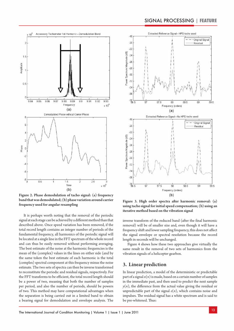
Some results from[7] are shown to demonstrate the possibilities. It involved vibrations from a gas turbine engine with two shafts, but the tacho signal for the high-speed (HS) shaft was from a geared auxiliary shaft at a lower speed for which the gear ratio was known only approximately. However, a lot of the speed fluctuation could be removed by resampling at equal phase angle increments of the auxiliary shaft. The phase variation of this shaft about the mean speed, determined by phase demodulation, is shown in Figure 2(b), while Figure 2(a) shows the original spectral peak corresponding to the first harmonic of the auxiliary shaft, which was demodulated to get this result.
After angular resampling, the 60th harmonic of the HS shaft could also be located in the vibration spectrum and this was used to calculate a new gear ratio for the order tracking. This gave an improvement in the separation of the lower harmonics of the HS shaft, but higher order harmonics (57-59) were not removed at all. The separation index was 0.2211. However, it was found that by progressively phase demodulating higher order shaft harmonics, a much better result could be obtained. Figure 3 shows how well the higher harmonics have been removed by two strategies, both giving almost the same result. In the first case, the auxiliary tacho signal was used to remove most of the speed fluctuation, after which the 141st shaft harmonic could be located in the vibration spectrum and demodulated to give further refinement. In the second case, the tacho signal was not used, but the speed correction was done in three steps: first the fundamental, then the 43rd harmonic, and finally the 141st harmonic of the HS shaft speed could be located and demodulated for further refinement. The separation indices for the two methods were 0.6917 and 0.6785, respectively.
Figure 1. Comb filter characteristic for eight synchronous averages[4]
The International Journal of Condition Monitoring | Volume 1 | Issue 1 | June 201113
SIGNAL PROCESSING | FEATURE
It is perhaps worth noting that the removal of the periodic signal at each stage can be achieved by a different method than that described above. Once speed variation has been removed, if the total record length contains an integer number of periods of the fundamental frequency, all harmonics of the periodic signal will be located at a single line in the FFT spectrum of the whole record and can thus be easily removed without performing averaging. The best estimate of the noise at the harmonic frequencies is the mean of the (complex) values in the lines on either side (and by the same token the best estimate of each harmonic is the total (complex) spectral component at this frequency minus the noise estimate. The two sets of spectra can then be inverse transformed to reconstitute the periodic and residual signals, respectively. For the FFT transforms to be efficient, the total record length should be a power of two, meaning that both the number of samples per period, and also the number of periods, should be powers of two. This method may have computational advantages when the separation is being carried out in a limited band to obtain a bearing signal for demodulation and envelope analysis. The
inverse transform of the reduced band (after the final harmonic removal) will be of smaller size and, even though it will have a frequency shift and lower sampling frequency, this does not affect the signal envelope or spectral resolution because the record length in seconds will be unchanged.
Figure 4 shows how these two approaches give virtually the same result in the removal of two sets of harmonics from the vibration signals of a helicopter gearbox.
3. Linear predictionIn linear prediction, a model of the deterministic or predictable part of a signal x(n) is made, based on a certain number of samples in the immediate past, and then used to predict the next sample y(n), the difference from the actual value giving the residual or unpredictable part of the signal e(n), which contains noise and impulses. The residual signal has a white spectrum and is said to be pre-whitened. Thus:
Figure 2. Phase demodulation of tacho signal: (a) frequency band that was demodulated; (b) phase variation around carrier frequency used for angular resampling
Figure 3. High order spectra after harmonic removal: (a) using tacho signal for initial speed compensation; (b) using an iterative method based on the vibration signal

The International Journal of Condition Monitoring | Volume 1 | Issue 1 | June 201114
FEATURE | SIGNAL PROCESSING
x(n) = − a(k) ⋅ x(n − k)k=1
p
∑ + e(n) ......................(4)
and y(n) is the first term on the right.The coefficients a(k) of the autoregressive (AR) model,
represented by y(n), can be obtained using the Yule-Walker equations, often using the so-called Levinson-Durban Recursion (LDR) algorithm[8]. A Fourier transform of Equation (4), with x(n) incorporated into the summation of the convolution term, leads to:
X ( f )A( f ) = E( f ) ..................................(5)
or
X ( f ) =E( f )
A( f ) .......................................(6)
which can be considered as the output X(f) of a system with transfer function A–1(f) when excited by the forcing function E(f). The AR transfer function is thus an all-pole filter, the poles corresponding to the roots of polynomial A(f). The forcing function E(f) is white, containing stationary white noise and impulses, and its time domain counterpart e(n) is said to be ‘pre-whitened’. Thus, removing the deterministic (discrete frequency) components leaves a pre-whitened version of the residual signal, which includes the bearing signal because of its randomness. Some flexibility in choosing what is removed is given by the order p of the model. Each discrete frequency will correspond in principle to one pole, and so the order is often chosen to be roughly twice the number of expected discrete frequencies. Another consideration is the longest period of the periodicity being removed. In gear diagnostics[9,10], the order p is chosen to be several periods of the gear mesh frequency, so as to remove it, but shorter than the rotation period of the gear so as not to remove fault pulses repeating every revolution.
Various criteria can be used for optimising the filter order. The literature[9] recommends the Akaike Information Criterion (AIC)[11] for gear diagnostics, which prevents the choice of too high an order while attempting to minimise the error power. In bearing diagnostics, the main aim is to maximise the impulsiveness of the
residual signal (assuming that this is dominated by the bearing fault) and in[12] it was shown that this could often be achieved with a very small order, using a kurtosis criterion instead of the AIC. Figure 5 shows a result from[12], where a model of order 4 (AR(4)) was able to remove the dominant masking of the gears while increasing the kurtosis from –0.04 to 5.7.
Where very large numbers of components are to be removed, for example both mesh harmonics and sidebands in gear spectra, the DRS method of Section 5 is probably better because of its efficiency and stability.
4. Self-adaptive noise cancellation (SANC)This method is based on the different correlation lengths of deterministic and random signals. It is an extension of the concept of adaptive noise cancellation, where a primary signal, containing a mixture of two components, can be separated into those two constituents using an adaptive filter fed with a reference signal containing only one[13]. The reference signal does not have to be identical to the relevant component, just coherent with it so that they are related by a linear transfer function, this being found by the adaptive filter. In self-adaptive noise cancellation, the primary signal must be a combination of deterministic and random components, and the reference signal is simply a delayed version of the primary signal.
This is illustrated in Figure 6, for the situation where the deterministic part is a gear signal and the random part a bearing signal. If the delay is made longer than the correlation length of the random part, the adaptive filter will only recognise the relationship between the primary signal and the delayed version of it, and by minimising the power of the residual signal (the random part) will find the appropriate transfer function, which is a delay.
Ho[14] shows that an iterative procedure for the calculation of
Figure 4. Power spectrum of: (a) order tracked signal showing two sets of harmonics; (b) residual signal obtained by setting the rotor-related harmonics to the mean of adjacent (noise) lines; and (c) residual signal obtained by subtracting the synchronous average
Figure 5. Use of AR model to remove gear masking from a gearbox signal with a bearing outer race fault: (a) raw signal; (b) linearly predicted part of AR(4) model; and (c) AR(4) residual (pre-whitened signal)

The International Journal of Condition Monitoring | Volume 1 | Issue 1 | June 201115
SIGNAL PROCESSING | FEATURE
the adaptive filter Wk is given by:
Wk+1 =Wk+2µ
nεkXk
(L +1)σ̂k
2 ................................(7)
where Wk = Vector of weight coefficients of the adaptive filter at the kth iteration
μn = Normalised convergence factor: 0 < μn < 1
μ = Convergence factor: µ =µn
(L +1)σ̂k
2
εk = Output error at kth iteration Xk = Vector of input values at kth iteration L = Order of the adaptive filter (L+1) = Number of filter coefficients !̂
k
2 = Exponential-averaged estimate of the input signal power at the kth iteration
and the output error εk is being minimised by a ‘least mean squares’ (LMS) operation[13]. It will converge to the minimum if the normalised convergence factor μn is chosen correctly. If it is too large, the result will oscillate and diverge, while if too small, the iteration process will take too long. The best choice may have to be arrived at by trial and error.
Some guidance is also required for the choice of the other parameters in the expression, and for the delay Δ. The order L is typically in the hundreds or even thousands where the number of sinusoids to be removed is large. An empirical study of the optimum choice of filter order was made in[15], and the major results (for a single family of equally-spaced harmonics or sidebands in the band being treated) are shown in Figure 7.
As mentioned above, the delay Δ should be longer than the correlation length of the random part of the signal. This will be of the order of the reciprocal of the minimum 3 dB bandwidth of resonance peaks in the signal spectrum, which may be estimated by inspection or by a knowledge of typical damping factors of modes in the frequency range of interest. The delay should be at least three times this value, but not much longer, because even though the correlation length of deterministic signals is theoretically infinite, there is some deterioration in practice, in
particular if minor speed fluctuations have not been removed. Where the random signal is dominated by rolling element
bearing fault signals, it is reasonable to assume that the random variation in period of the fault pulses will be of the order of 1%, in which case the correlation length will correspond to 100 periods of the centre frequency of the band to be demodulated, and so a delay of 300 periods is appropriate. If the band is at 10 kHz, for example, this will correspond to about 30 ms.
It is in fact one of the advantages of the SANC method, over the DRS method discussed in the next section, that the adaptive filter can accommodate slow changes in the signal over periods greater than the filter order. Otherwise, the DRS method will normally be more efficient, though giving very similar results.
5. Discrete/random separation (DRS)This method also finds the coherent relationship between the signal and a delayed version of itself, but because it is done in the frequency domain, it is much more efficient[16]. The frequency response function (FRF) between the original and delayed signals is obtained using a formulation similar to the so-called H1 FRF used in modal analysis. This is defined as:
H1( f ) =
E Gb ( f )Ga * ( f )[ ]E Ga ( f )Ga * ( f )[ ]
=Gab ( f )
Gaa ( f ) ..................(8)
where Ga(f) is the spectrum of the input, Gb(f) is the spectrum of the output, Gab(f) is the cross spectrum and Gaa(f) is the input autospectrum. H1 is ideal when the input signal has little noise, since noise averages out of the cross spectrum. However, in DRS the input and output signals contain the same amount of noise, and in[16] it is shown that the amplitude of the separation filter (which should be unity for discrete frequency components and zero for noise) is given by:
ρN
2W ( f )
2
ρN
2W ( f )
2+1
......................................(9)
where ρ = SNR (signal-to-noise ratio), N is the transform size, and W(f) is the Fourier transform of the window used, scaled to a maximum value of 1 in the frequency domain. Even for a SNR as low as 10–2 (–20 dB), this gives a value of 0.7 for N = 512. This filter can be applied in the frequency domain, which is much more efficient than applying convolutive filters in the time domain, as for SANC (or linear prediction). If the amplitude of the FRF (filter characteristic) is used, it corresponds to a non-causal filter which does not alter the phase of filtered components. Because the filter is applied blockwise in the frequency domain, and all FFT operations are circular, the so-called ‘overlap/add’ method must be used for the application of the filter, basically discarding half the result each time, but it is still much more efficient than time domain convolutions, in particular for high order filters. The filter is determined by averaging over the whole time record first and then applied by post-processing, so in general speed fluctuations must first be removed by order tracking[5].
Figure 8 shows the result of applying the DRS procedure to a complicated signal from a helicopter gearbox. Only a zoomed section of the spectrum is shown for clarity, but the whole
Figure 7. Minimum filter order versus number of discrete spectrum components
Figure 6. Schematic diagram of self-adaptive noise cancellation used for removing periodic interference

The International Journal of Condition Monitoring | Volume 1 | Issue 1 | June 201116
FEATURE | SIGNAL PROCESSING
(normalised) spectrum range from 0-0.5 times the sampling frequency was processed in one operation.
Figure 8(a) shows the original spectrum, with a mixture of different discrete frequency families protruding above the noise level by varying amounts. Figure 8(b) shows the generated H1 filter, which can be seen to be close to 1 where the discrete frequencies protrude most from the noise, and near zero for the noise in between. Figure 8(c) shows that when this filter is applied back on the original signal, the noise level has been reduced by approximately 20 dB. Figure 8(d) shows that the residual noise signal left after subtraction of the deterministic part has some notches in the vicinity of the discrete filters, but this does not normally affect the envelope of the signal if the purpose is to perform envelope analysis for bearing diagnostics.
Figure 9 shows the result of applying DRS to the same signal as Figure 4, where order tracking has been applied to remove speed fluctuations, but where there was not an integer number of samples per period of each harmonic family. Notches can be seen in the noise spectrum.
Figure 10 illustrates the application to bearing diagnostics, in a case where the bearing fault signal was only visible in the original time signal at some isolated peaks[16]. The fault was in a rolling element (ball) and so the fault pulses were strongly modulated at cage speed, the basic period being about 2½ times the shaft rotation period.
6. Cepstral methodThere are a number of versions of the cepstrum, but the fundamental definition can be said to be the inverse Fourier transform of a logarithmic spectrum as in Equation (10):
C(τ ) = ℑ
−1 log F( f )( ){ } ..........................(10)
The spectrum can be obtained from the forward Fourier transform of a time signal, in which case it will be complex, and can be expressed in terms of its amplitude and phase at each frequency as:
F( f ) = ℑ f (t){ } = A( f )e jφ ( f ) ...................(11)
If the phase is retained, the logarithmic spectrum has log amplitude as real part and phase as imaginary part, and the so-called ‘complex cepstrum’ is obtained as:
C
c(τ ) = ℑ−1 ln A( f )( ) + jφ( f ){ } .................(12)
In order to calculate the complex cepstrum, the phase φ(f)must be a continuous function of frequency. This is possible for analytic functions such as FRFs, but not in general for forcing functions or response functions where the forcing function is modified by a transfer function. Forcing functions often consist of a mixture of deterministic discrete frequency components, where phase is undefined between these components, and noise, whose phase is discontinuous with frequency. Note that despite its name the complex cepstrum is actually real, since the log amplitude is even, while the phase is odd.
If the phase is disregarded, as in Equation (13), the so-called ‘real cepstrum’ is obtained:
C
r(τ ) = ℑ
−1 ln A( f )( ){ } ............................(13)
This has the advantage that the phase does not have to be unwrapped and it can be applied to forcing and response signals. On the other hand, it is only reversible to the spectrum, rather
Figure 8. Application of DRS to a helicopter gearbox vibration signal: (a) original spectrum (zoomed); (b) amplitude characteristic of filter; (c) spectrum of deterministic part; (d) spectrum of random part
Figure 9. Spectrum of signal of Figure 4 after removal of all discrete frequency components using DRS
Figure 10. Example of a ball fault in a gearbox: (a) measured vibration signal; (b) extracted periodic part; (c) extracted non-deterministic part[16]
The International Journal of Condition Monitoring | Volume 1 | Issue 1 | June 201117
SIGNAL PROCESSING | FEATURE
than a time signal. It can also be applied to smoothed autospectra, which will often reduce noise. If the log autospectrum (power spectrum) is used, the squaring of the amplitude leads to a trivial scaling of Equation (13) by a factor of 2, and the result is often called the ‘power cepstrum’. In fact, the originally proposed cepstrum[17] was a power cepstrum defined as the power spectrum of the logarithm of the power spectrum, but this was not reversible, even to the spectrum. Note that when the autospectrum is used, the only difference between the cepstrum and the autocorrelation function is the logarithmic operation, but the latter gives the considerable benefit that forcing function and transfer function are related by addition rather than convolution in the response.
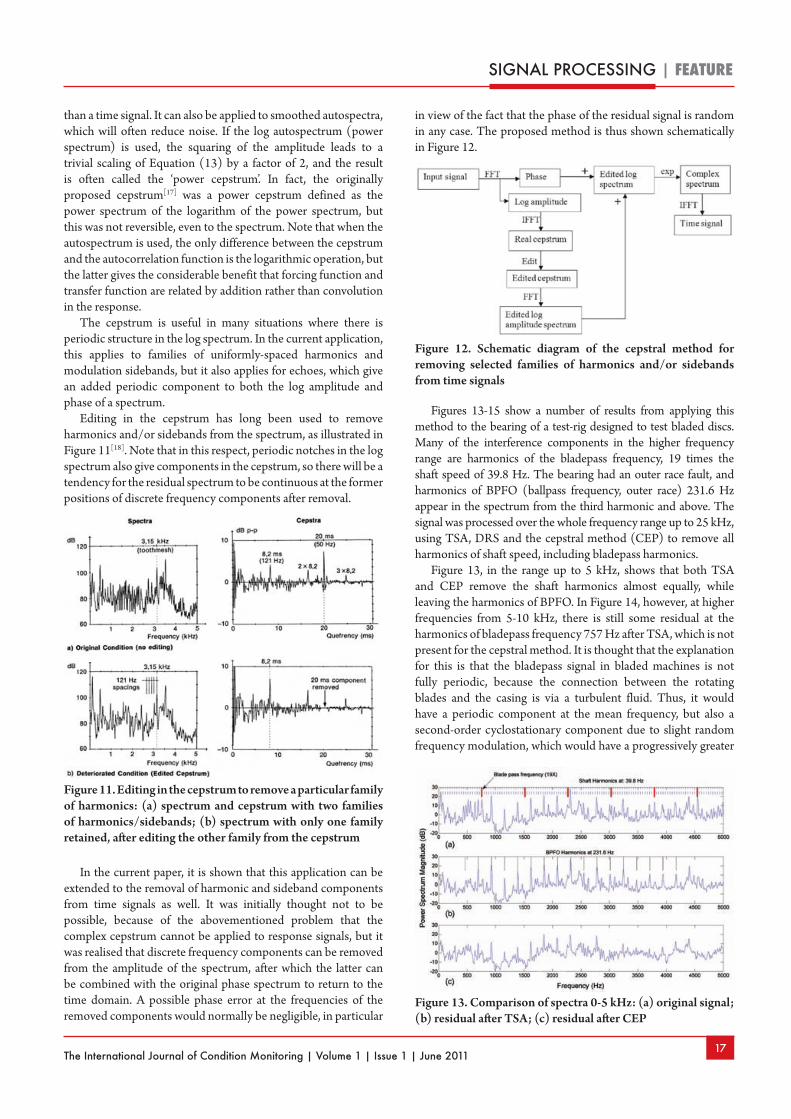
The cepstrum is useful in many situations where there is periodic structure in the log spectrum. In the current application, this applies to families of uniformly-spaced harmonics and modulation sidebands, but it also applies for echoes, which give an added periodic component to both the log amplitude and phase of a spectrum.
Editing in the cepstrum has long been used to remove harmonics and/or sidebands from the spectrum, as illustrated in Figure 11[18]. Note that in this respect, periodic notches in the log spectrum also give components in the cepstrum, so there will be a tendency for the residual spectrum to be continuous at the former positions of discrete frequency components after removal.
In the current paper, it is shown that this application can be extended to the removal of harmonic and sideband components from time signals as well. It was initially thought not to be possible, because of the abovementioned problem that the complex cepstrum cannot be applied to response signals, but it was realised that discrete frequency components can be removed from the amplitude of the spectrum, after which the latter can be combined with the original phase spectrum to return to the time domain. A possible phase error at the frequencies of the removed components would normally be negligible, in particular
in view of the fact that the phase of the residual signal is random in any case. The proposed method is thus shown schematically in Figure 12.
Figures 13-15 show a number of results from applying this method to the bearing of a test-rig designed to test bladed discs. Many of the interference components in the higher frequency range are harmonics of the bladepass frequency, 19 times the shaft speed of 39.8 Hz. The bearing had an outer race fault, and harmonics of BPFO (ballpass frequency, outer race) 231.6 Hz appear in the spectrum from the third harmonic and above. The signal was processed over the whole frequency range up to 25 kHz, using TSA, DRS and the cepstral method (CEP) to remove all harmonics of shaft speed, including bladepass harmonics.
Figure 13, in the range up to 5 kHz, shows that both TSA and CEP remove the shaft harmonics almost equally, while leaving the harmonics of BPFO. In Figure 14, however, at higher frequencies from 5-10 kHz, there is still some residual at the harmonics of bladepass frequency 757 Hz after TSA, which is not present for the cepstral method. It is thought that the explanation for this is that the bladepass signal in bladed machines is not fully periodic, because the connection between the rotating blades and the casing is via a turbulent fluid. Thus, it would have a periodic component at the mean frequency, but also a second-order cyclostationary component due to slight random frequency modulation, which would have a progressively greater
Figure 11. Editing in the cepstrum to remove a particular family of harmonics: (a) spectrum and cepstrum with two families of harmonics/sidebands; (b) spectrum with only one family retained, after editing the other family from the cepstrum
Figure 12. Schematic diagram of the cepstral method for removing selected families of harmonics and/or sidebands from time signals
Figure 13. Comparison of spectra 0-5 kHz: (a) original signal; (b) residual after TSA; (c) residual after CEP
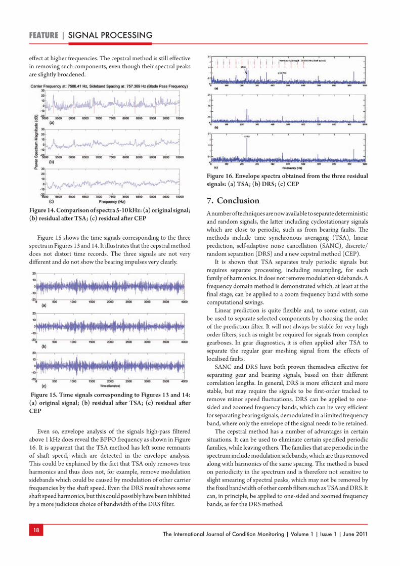
The International Journal of Condition Monitoring | Volume 1 | Issue 1 | June 201118
FEATURE | SIGNAL PROCESSING
7. ConclusionA number of techniques are now available to separate deterministic and random signals, the latter including cyclostationary signals which are close to periodic, such as from bearing faults. The methods include time synchronous averaging (TSA), linear prediction, self-adaptive noise cancellation (SANC), discrete/random separation (DRS) and a new cepstral method (CEP).
It is shown that TSA separates truly periodic signals but requires separate processing, including resampling, for each family of harmonics. It does not remove modulation sidebands. A frequency domain method is demonstrated which, at least at the final stage, can be applied to a zoom frequency band with some computational savings.
Linear prediction is quite flexible and, to some extent, can be used to separate selected components by choosing the order of the prediction filter. It will not always be stable for very high order filters, such as might be required for signals from complex gearboxes. In gear diagnostics, it is often applied after TSA to separate the regular gear meshing signal from the effects of localised faults.
SANC and DRS have both proven themselves effective for separating gear and bearing signals, based on their different correlation lengths. In general, DRS is more efficient and more stable, but may require the signals to be first-order tracked to remove minor speed fluctuations. DRS can be applied to one-sided and zoomed frequency bands, which can be very efficient for separating bearing signals, demodulated in a limited frequency band, where only the envelope of the signal needs to be retained.
The cepstral method has a number of advantages in certain situations. It can be used to eliminate certain specified periodic families, while leaving others. The families that are periodic in the spectrum include modulation sidebands, which are thus removed along with harmonics of the same spacing. The method is based on periodicity in the spectrum and is therefore not sensitive to slight smearing of spectral peaks, which may not be removed by the fixed bandwidth of other comb filters such as TSA and DRS. It can, in principle, be applied to one-sided and zoomed frequency bands, as for the DRS method.
effect at higher frequencies. The cepstral method is still effective in removing such components, even though their spectral peaks are slightly broadened.
Figure 15 shows the time signals corresponding to the three spectra in Figures 13 and 14. It illustrates that the cepstral method does not distort time records. The three signals are not very different and do not show the bearing impulses very clearly.
Even so, envelope analysis of the signals high-pass filtered above 1 kHz does reveal the BPFO frequency as shown in Figure 16. It is apparent that the TSA method has left some remnants of shaft speed, which are detected in the envelope analysis. This could be explained by the fact that TSA only removes true harmonics and thus does not, for example, remove modulation sidebands which could be caused by modulation of other carrier frequencies by the shaft speed. Even the DRS result shows some shaft speed harmonics, but this could possibly have been inhibited by a more judicious choice of bandwidth of the DRS filter.
Figure 14. Comparison of spectra 5-10 kHz: (a) original signal; (b) residual after TSA; (c) residual after CEP
Figure 15. Time signals corresponding to Figures 13 and 14: (a) original signal; (b) residual after TSA; (c) residual after CEP
Figure 16. Envelope spectra obtained from the three residual signals: (a) TSA; (b) DRS; (c) CEP

The International Journal of Condition Monitoring | Volume 1 | Issue 1 | June 201119
SIGNAL PROCESSING | FEATURE
8. AcknowledgementThis research has been supported by the Australian Government’s Defence Science and Technology Organisation, through the DSTO Centre of Expertise at UNSW.
9. References1. J Antoni, ‘Cyclostationarity by examples’, Mechanical Systems
and Signal Processing, 23, pp 987-1036, 2009.2. J Antoni and R B Randall, ‘Differential diagnosis of gear and
bearing faults’, ASME Journal of Vibration and Acoustics, 124, pp 165-171, 2002.
3. S Braun, ‘The extraction of periodic waveforms by time domain averaging’, Acoustica, 23 (2), pp 69-77, 1975.
4. P D McFadden, ‘A revised model for the extraction of periodic waveforms by time domain averaging’, Mechanical Systems and Signal Processing, 1 (1), pp 83-95, 1987.
5. P D McFadden, ‘Interpolation techniques for time domain averaging of gear vibration’, Mechanical Systems and Signal Processing, 3 (1), pp 87-97, 1989.
6. F Bonnardot, M El Badaoui, R B Randall, J Danière and F Guillet, ‘Use of the acceleration signal of a gearbox in order to perform angular resampling (with limited speed fluctuation)’, Mechanical Systems and Signal Processing, 19, pp 766-785, 2005.
7. M D Coats, N Sawalhi and R B Randall, ‘Extraction of tacho information from a vibration signal for improved synchronous averaging’, in: Proceedings of Acoustics Australia 2009, Adelaide, Australia, 23-25 November, 2009.
8. M S Kay and S L Marple, ‘Spectrum analysis – a modern perspective’, Proc IEEE, 69 (11), pp 1380-1419, 1981.
9. W Wang and A K Wong, ‘Autoregressive model-based gear fault diagnosis’, Trans ASME, Journal of Vibration and
Acoustics, 124, pp 172-179, 2002.10. H Endo and R B Randall, ‘Enhancement of
autoregressive model-based gear tooth fault detection technique by the use of minimum entropy deconvolution filter’, Mechanical Systems and Signal Processing, 21(2), pp 906-919, 2007.
11. H Akaike, ‘Fitting autoregressive models for prediction’, Ann Inst Math, 21, pp 243-247, 1969.
12. N Sawalhi, ‘Rolling element bearings: diagnostics, prognostics and fault simulations’, PhD Dissertation, University of New South Wales, 2007. Available from UNSW Library at www.library.unsw.edu.au/~thesis/adt-NUN/public/adt-NUN20070704.105600/index.html
13. B Widrow and S Stearns, Adaptive Signal Processing, Prentice-Hall, Englewood Cliffs NJ, pp 349-351, 1985.
14. D Ho, ‘Bearing diagnostics and self-adaptive noise cancellation’, PhD Dissertation, UNSW, 2000.
15. D Ho and R B Randall, ‘Effects of time delay, order of FIR filter and convergence factor on self-adaptive noise cancellation’ International Conference on Sound and Vibration (ICSV5), Adelaide, 1997.
16. J Antoni and R B Randall, ‘Unsupervised noise cancellation for vibration signals: part II – a novel frequency-domain algorithm’, Mechanical Systems and Signal Processing, 18, pp 103-117, 2004.
17. B P Bogert, M J R Healy and J W Tukey, ‘The quefrency alanysis of time series for echoes: cepstrum, pseudo-autocovariance, cross-cepstrum and saphe cracking’, in: Proc of the Symp on Time Series Analysis, M Rosenblatt (Ed), Wiley, NY, pp 209-243, 1963.
18. R B Randall, ‘Cepstrum Analysis’, in: Encyclopedia of Vibration, Eds D Ewins, S S Rao and S Braun, Academic Press, London, 2001.

The International Journal of Condition Monitoring | Volume 1 | Issue 1 | June 201120
FEATURE | MCSA
This paper presents the results of an experimental approach used to arrive at the detection of faults in brushless DC motor-based electromechanical linear actuators using motor current signature analysis (MCSA). The failure modes for these systems transcend electrical, mechanical and electronic systems and are masked by external forces and the dynamic properties of control systems, making it difficult to use model-based condition monitoring techniques. Generally, these systems are critical for mission accomplishment and are stored for longer durations before operation, so a comprehensive health monitoring strategy is required for their fault-free operation. The aim of this paper is to identify fault signatures due to more practically observed faults, such as gear tooth breakage, and errors in gear mounting, such as eccentricity and clearance. The paper also deals with identifying faults in the satellite roller screw, considering improper preload and backlash. Vibration signatures are used as a reference to validate the MCSA. The effect of load on the motor current signatures and their comparison with vibration signatures is also presented. MCSA signatures of faults in the satellite roller screw are dealt with in the paper for the first time.
Keywords: BLDC motor, condition monitoring, electromechanical linear actuator, motor current signature analysis.
1. IntroductionCondition monitoring is defined as a technique or a process of monitoring the operating characteristics of a machine in such a way that the changes and trends of the monitored characteristics can be used to predict the need for maintenance before serious deterioration. Electrical motor-based reliable power-by-wire actuation systems for both aeronautical and space applications have been sought recently to eliminate hydraulic and pneumatic systems and thus improve safety, efficiency, reliability and maintainability. Brushless DC (BLDC) motors further enhance the advantages, such as linear torque speed characteristics, better cooling, sparkless
commutation etc. Electromechanical actuators (EMLA) on board aircraft are powered from the aircraft electrical system, eliminating the need for central hydraulic and pneumatic systems. Efficient torque amplification has made the electromechanical linear actuators more popular than rotary actuators.
Motor current signature analysis (MCSA) has been a recent addition as a non-intrusive and easy-to-measure condition monitoring technique. The application of MCSA to gear condition monitoring has been investigated by Mohanty and Kar(1,2), applied to induction motor-driven systems using MCSA. The MCSA was used to detect the fault signatures as sidebands to supply line frequencies in the case of induction motors. Mohanty and Kar(3) applied amplitude demodulation and frequency demodulation to the current drawn by the induction motor for detecting the rotating shaft frequencies and GMFs, respectively. Discrete wavelet transform was applied to the demodulated current signal for denoising and removing the intervening neighbouring features. The spectrum of a particular level, which comprises the GMFs, is used for one and two teeth removal gear fault detection. All the above work has been carried out on
Condition monitoring of brushless DC motor-based electromechanical linear actuators using motor current signature analysisG Sreedhar Babu, A Lingamurthy and A S Sekhar
G Sreedhar Babu and A Lingamurthy are Scientists at the Control Systems Laboratory, RCI, Hyderabad, India.
A S Sekhar* is a Professor in the Machine Design Section, Department of Mechanical Engineering, Indian Institute of Technology Madras, Chennai 600 036, India.
*Corresponding author. Email: [email protected]
Notation A Amplitude of the position command issued to actuatorBLDC Brushless direct current motor DAC Data acquisition computerDC Direct currentEMLA Electromechanical linear actuatorFFT Fast Fourier transformFRA Frequency response analyserGMF Gear mesh frequencyG1 Gear with one tooth removed fault induced G2 Gear with two teeth removed fault induced HALF High-amplitude low-frequency command LVDT Linear variable differential transducerMCSA Motor current signature analysisPWM Pulse width modulation Ramp Position command with uniform velocity to arrive at frictional torqueSine 195 Position command, 5 cycles of sine wave, 9 V (27 mm) amplitude, frequency 1 Hz to obtain harmonic responseSRS Satellite roller screwStep 9 Position step command of 9 V electrical amplitude (27 mm mechanical stroke) STFT Short-time Fourier transformω Motor’s rotor frequency in HzΩ Frequency of linear position command given to actuator in Hz
Submitted 11.08.10 Accepted 02.12.10

The International Journal of Condition Monitoring | Volume 1 | Issue 1 | June 201121
MCSA | FEATURE
induction motors. In the present work, which is along similar lines, and also in the case of the BLDC motors, the current is free from supply line harmonics making MCSA more appropriate.
Rajagopalan et al(4) investigated the effect of several potential rotor faults on the current spectrum of BLDC motors to develop an effective condition monitoring scheme. The effect of load unbalances, misalignments and varying load torques on the diagnosis of such machines was investigated and experimentally concluded that current signature analysis could be a viable tool for diagnosing the condition of BLDC machines. However, their work was confined to electrical faults of motors running continuously.
The output shafts of electromechanical linear actuators oscillate about a mean position and can never run in a steady state condition as they have a limited stroke, unlike the rotary actuators which can run in a stationary condition. Rajagopalan et al(5) have discussed analytic wavelet transform of the stator-current signal and proposed methods for detecting dynamic eccentricity in BLDC motors operating under rapidly varying speed and load conditions. They devised a method that works over a wide speed range of motor operation and provides an effective and robust way of detecting rotor faults such as dynamic eccentricity in BLDC motors. Rajagopalan et al(6) have proposed methods using windowed Fourier ridges and Wigner-Ville-based distributions for the detection of rotor faults in BLDC motors operating under continuous non-stationary conditions. Rajagopalan et al(7) used the Wigner-Ville family of time-frequency distributions as an alternative to short-time Fourier transforms (STFTs) and wavelets for the diagnostics of rotor faults in a BLDC motor. All the works reported concentrate on motors driving rotary actuators and faults within the BLDC motor. Actuator level faults such as faults in transmission elements external to the BLDC motor were not considered. The present paper deals with faults in the actuator external to the motor, transmitted to the motor through the transmission mechanism.
Byington et al(8) presented a model-based approach to prognostics and health management that applies physical modelling and advanced parametric identification techniques, along with fault detection and failure prediction algorithms, for flight control actuator fault detection and failure prediction. The kinematic and dynamic models of a similar linear electric actuator were presented(9). The kinematic model was obtained by geometric analysis. The dynamic model was obtained with Lagrange’s methodology for a linear actuator used in an elbow prosthesis. Juricic et al(10) presented a system for diagnosing faults in a valve actuator driven by a BLDC motor during offline preflight tests.
From the above survey, it is evident that a good amount of work has been done in the field of condition monitoring of BLDC motors and induction motors up to the motor level only, revealing their importance and utility. Kim(11) presented modelling of BLDC motor-based EMLA for robot manipulators and described dynamic and fault analysis of the actuator using the model. Jayakumar and Das(12) proposed a simulation-based fault detection scheme. It uses a single Luenberger observer-based scheme for the detection and isolation of incipient sensor faults in a practical electromechanical flight actuator used in a flight control actuation system. However, this is based on simulation rather than experimentation. The research carried out by Alstom Power on the development and validation of an observer-based
fault detection identification and accommodation (FDIA) system for an electromechanical actuator on laboratory-scale plant has also been discussed(13). Skormin et al(14) presented a mathematical model describing the dynamics of a self-contained flight control actuator. A diagnostic model of the actuator, intentionally sensitive to particular types of failure, is defined. This work is in the field of mathematical models; verification is done in simulation and no experimental comparison is presented.
The present work concentrates on the condition monitoring of an electromechanical linear actuator (EMLA), which differs from the above discussed systems in terms of operation and utility. The EMLAs are extensively used in aerospace applications and are generally inaccessible. These EMLAs cannot be run in a stationary condition, unlike the systems discussed earlier, since linear stroke is limited and they are basically closed-loop feedback systems.
Although the need for condition-based maintenance is clearly recognised, the problem of detecting faults and predicting failures in actuators is complex and difficult to solve. The failure modes for these systems transcend electrical, mechanical and fluid systems and can be masked by external forcing due to aerodynamic loads and other varying forces. The dynamic properties of control systems can further mask the developing faults until the damage becomes excessive and dangerous enough to trip a system fault monitor.
The aim of the present study is to devise an experimental methodology for the condition monitoring of closed-loop BLDC motor-based electromechanical linear actuators used in aerospace applications. The study is to identify MCSA fault signatures due to more practical faults such as gear tooth breakage and errors in gear mounting such as eccentricity and clearance. A satellite roller screw (SRS), a popular rotary-to-linear motion conversion mechanism, is used in such systems. The paper also deals with fault signatures in SRS, considering errors such as improper preload and backlash. MCSA signatures of faults in the satellite roller screw are dealt with in the paper for the first time. Unlike the previous studies, the condition monitoring aspects are based on an experimental approach. The present experimental study is only a step towards building a diagnosis model of typical faults. The novelty of the paper is to use the MCSA technique on a BLDC motor EMLA for identification of faults external to the motor and transmitted to the motor, based on an experimental approach.
The organisation of the subsequent sections is as follows. In Section 2, the paper introduces the system under experimentation, followed by explaining generally occurring faults in the system. The experimental details are presented in Section 3. Here, different sensors with the corresponding instrumentation and various tests planned are discussed. In Section 4, the calculated values of frequencies expected from the spectra due to the system geometry and a detailed explanation of closed-loop systems are presented. The experimentation is done in two phases. In the first phase, experimentation is carried out to arrive at a sampling frequency, comparison of vibration and MCSA fault signatures and the affect of load on MCSA and vibration signatures, as explained in Sections 5.1 and 5.2. In the second phase, the MCSA signatures of more practical faults in the gear train and satellite roller are discussed in detail in Sections 5.3 to 5.6. In these Sections, only MCSA is considered.
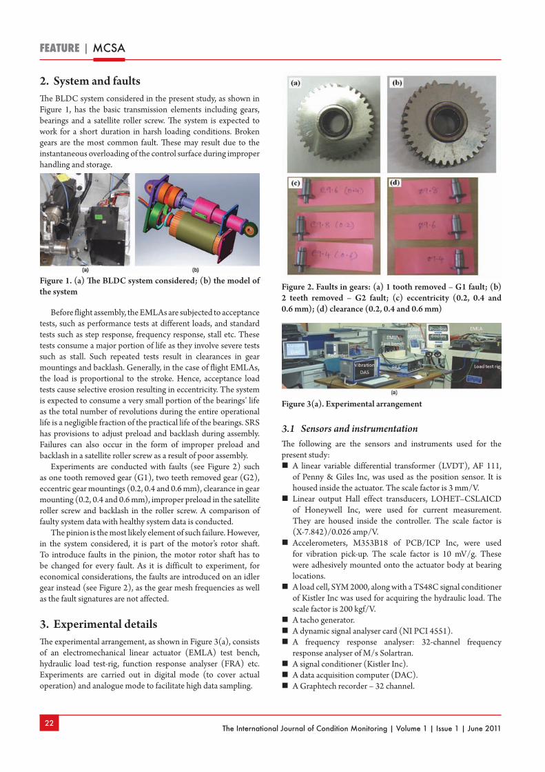
The International Journal of Condition Monitoring | Volume 1 | Issue 1 | June 201122
FEATURE | MCSA
2. System and faultsThe BLDC system considered in the present study, as shown in Figure 1, has the basic transmission elements including gears, bearings and a satellite roller screw. The system is expected to work for a short duration in harsh loading conditions. Broken gears are the most common fault. These may result due to the instantaneous overloading of the control surface during improper handling and storage.
Before flight assembly, the EMLAs are subjected to acceptance tests, such as performance tests at different loads, and standard tests such as step response, frequency response, stall etc. These tests consume a major portion of life as they involve severe tests such as stall. Such repeated tests result in clearances in gear mountings and backlash. Generally, in the case of flight EMLAs, the load is proportional to the stroke. Hence, acceptance load tests cause selective erosion resulting in eccentricity. The system is expected to consume a very small portion of the bearings’ life as the total number of revolutions during the entire operational life is a negligible fraction of the practical life of the bearings. SRS has provisions to adjust preload and backlash during assembly. Failures can also occur in the form of improper preload and backlash in a satellite roller screw as a result of poor assembly.
Experiments are conducted with faults (see Figure 2) such as one tooth removed gear (G1), two teeth removed gear (G2), eccentric gear mountings (0.2, 0.4 and 0.6 mm), clearance in gear mounting (0.2, 0.4 and 0.6 mm), improper preload in the satellite roller screw and backlash in the roller screw. A comparison of faulty system data with healthy system data is conducted.
The pinion is the most likely element of such failure. However, in the system considered, it is part of the motor’s rotor shaft. To introduce faults in the pinion, the motor rotor shaft has to be changed for every fault. As it is difficult to experiment, for economical considerations, the faults are introduced on an idler gear instead (see Figure 2), as the gear mesh frequencies as well as the fault signatures are not affected.
3. Experimental detailsThe experimental arrangement, as shown in Figure 3(a), consists of an electromechanical linear actuator (EMLA) test bench, hydraulic load test-rig, function response analyser (FRA) etc. Experiments are carried out in digital mode (to cover actual operation) and analogue mode to facilitate high data sampling.
3.1 Sensors and instrumentation The following are the sensors and instruments used for the present study: n A linear variable differential transformer (LVDT), AF 111,
of Penny & Giles Inc, was used as the position sensor. It is housed inside the actuator. The scale factor is 3 mm/V.
n Linear output Hall effect transducers, LOHET–CSLAICD of Honeywell Inc, were used for current measurement. They are housed inside the controller. The scale factor is (X-7.842)/0.026 amp/V.
n Accelerometers, M353B18 of PCB/ICP Inc, were used for vibration pick-up. The scale factor is 10 mV/g. These were adhesively mounted onto the actuator body at bearing locations.
n A load cell, SYM 2000, along with a TS48C signal conditioner of Kistler Inc was used for acquiring the hydraulic load. The scale factor is 200 kgf/V.
n A tacho generator. n A dynamic signal analyser card (NI PCI 4551).n A frequency response analyser: 32-channel frequency
response analyser of M/s Solartran.n A signal conditioner (Kistler Inc).n A data acquisition computer (DAC).n A Graphtech recorder – 32 channel.
Figure 1. (a) The BLDC system considered; (b) the model of the system Figure 2. Faults in gears: (a) 1 tooth removed – G1 fault; (b)
2 teeth removed – G2 fault; (c) eccentricity (0.2, 0.4 and 0.6 mm); (d) clearance (0.2, 0.4 and 0.6 mm)
Figure 3(a). Experimental arrangement

The International Journal of Condition Monitoring | Volume 1 | Issue 1 | June 201123
MCSA | FEATURE
3.1.1 EMLA test benchThe EMLA has provision for both MIL-STD bus digital and RS-232-based analogue mode operation. The EMLA operates in digital mode in service. This mode of testing was carried out using a dedicated EMLA test bench. The test bench has a limitation of data sampling at 100 Hz, which is not sufficient for certain tests such as step command. Thus, analogue mode testing was carried out using a standard 32-channel frequency response analyser. A patch card was made to enable the analogue mode testing.
The test bench, as shown in Figure 3(a), is a unified tool to configure the EMLA system, perform its self-check and evaluate its performance. It facilitates testing by subjecting the EMLA to specified types of position commands. Feedback is acquired from the actuators, converted to appropriate units and displayed. It encloses a function generator card built into a computer to generate the required position commands and communicate it to the electromechanical actuator in 10 ms intervals over MIL-STD-1553 in digital mode.
The system acquires feedback from the LVDT to determine the position of the output shaft, from the tacho generator to determine the angular velocity of the rotor, and from the Hall effect current sensors to determine motor current. Electronic commutation is done by decoding the data acquired from the Hall effect sensors. Based on the feedback from the BLDC motor, the current, velocity and position control loops are executed to deliver power to the motor. The power supply is through batteries. The test bench software facilitates the issuing of position commands as analogue signals of a specific type using a dynamic signal analyser card (NI PCI 4551) interfaced to ADC channel. It also logs the received data and stores it. It is also provided with user-friendly GUI.
The test bench consists of a DC power supply, industrial PC, test-jig, associated software and a display system. The EMLA test-jig serves as a unified tool to configure the EMLA system. It is used to interface the EMLA with analogue mode and digital mode inputs and also to control the power supply to the system. It serves as an interface medium between the input commands from the PC to the EMLA and provision to monitor the feedback signals received from the controller.
3.1.2 Load test-rig The load test-rig is shown in Figure 3(b). It has fixtures to hold firmly the EMLA during the test. It has both spring and hydraulic loading capabilities. It encloses the pump motor package, hydraulic circuitry, control valves, fixtures, power supply unit, load cells, position sensor, signal conditioner for load position and display system. Only hydraulic loading was used. The pump
motor package is based on a three-phase induction motor of 2 hp. The hydraulic loading system has the capability of applying loads in the range from 80 kgf to 1800 kgf. The motor used is a three-phase 2 hp induction motor of speed 1440 r/min. A 2 ton load cell SYM 2000 and TS48C signal conditioner of Kistler Inc are used for data acquisition.
The hydraulic actuator is firmly fixed on the test bench with the necessary mechanical and electrical connections. The EMLA is electrically connected to the controller, which is the interface. The current and other parameters, such as position command, position feedback, velocity feedback and hydraulic load, are tapped from the test bench to the recorder and then passed to the data acquisition computer (DAC).
3.2 Different tests Figure 4 shows the schematic diagram of the testing procedure. A 1 Hz sine command of five cycles for a full stroke (28 mm) is given and the smooth operation of the actuator is ensured. Hydraulic loading is applied by using the hydraulic load test-rig and proper loading is ensured from the load cell display/data. All data acquisition systems are started and the required position command is issued to the actuator through the controller using the test bench. After the test is over, all data acquisition systems are stopped. The hydraulic loading is withdrawn and the actuator is powered off. All the data acquired is forwarded to the DAC for offline analysis. Experimentation is done at a very low frequency (50 mHz), full stroke command of (± 30 mm) to arrive at a quasi-stationary process to facilitate the use of FFT and to cover the total working range of components. The tests are conducted in no load, 200 kgf load and 500 kgf loading conditions. The sampling frequency used for vibration is 10240 Hz (integral power of 2). All the data, such as current, commands, feedbacks, loads etc, are acquired through a 32-channel Graphtech recorder with different sampling frequencies depending upon the commands and durations of tests conducted. The EMLA test bench has a limitation to the sampling frequency of 1 mHz. So, wherever high sampling frequencies are demanded, the testing is done in the analogue mode using a frequency response analyser (Solartran). The following list gives the different experimental tests conducted and the reasons for conducting such tests.n Step response test: Gives the most information about the
system in terms of raise time, settling time, peak overshoot and steady state positional error, which gives an idea of linearity and order of the system.
n Ramp test: Gives the fidelity of the system. Gives the capability of the system for velocity inputs and velocity error, damping etc.
n Harmonic response test: The response of the system to sinusoidal input at a signal frequency.
n Frequency response test: 20-1 Hz sinusoidal sweep at 10% FS. Gives magnitude and phase as a function of frequency (Bode plot).
n High-amplitude and low-frequency test: Covers the overall transmission system at a quasi-steady-state and gives an idea of localised effects.
n Low-amplitude low-frequency test: Gives an idea of the non-linearities of the system such as threshold, backlash, dead band etc, due to the absence of inertial effects.Figure 3(b). Load test rig

The International Journal of Condition Monitoring | Volume 1 | Issue 1 | June 201124
FEATURE | MCSA
4. Faults and expected frequenciesThe system considered is a BLDC motor-driven electromechanical actuator whose schematic is shown in Figure 5(a), where the BLDC motor drives a roller screw through a spur gear train of reduction ratio 1:2. The satellite roller screw (SRS) has a lead of 5 mm/rev, converting the rotary motion of the BLDC motor to the linear motion of the output shaft. The actuator is commanded with a linear position requirement.
A typical calculation of motor running frequency (ω) for a translation typical command shown in Figure 5(b) and the corresponding gear mesh frequency are given as: n No-load, high amplitude (27 mm), low-frequency (50 mHz)
command datan The frequency of command (Ω) = 50 e-3 Hzn Command amplitude (A) = 27 mmn Rotational speed of motor (ω) = A*Ω*cos Ωt/2.5 = 0.54 Hzn Gear mesh frequency (GMF) = nX ω = 8.64 Hz
From the example, it can be observed that the spectrum is expected to have peaks at harmonics of 8.64 Hz and sidebands at harmonics of 0.54 Hz. The frequencies of major concern that are expected to be visible in the current/vibration spectrum are: n Current pulse width modulation (PWM) frequency: 12.5 kHzn Motor rotating frequency: X Hzn Gear mesh frequency: 16X Hzn Supply line frequency (in hydraulic loading): 50 Hzn Hydraulic motor frequency: 23.5 Hz
The characteristic frequencies of the satellite roller screw (SRS) are also expected. As the geometry of the satellite roller screw is analogous to a roller bearing, the corresponding frequencies are calculated using the standard formulae. These frequencies for the SRS are estimated and more details are given in Section 5. The frequencies relating to other transmission elements such as bearings are also calculated for reference.
The frequency selection was based on the Nyquest sampling frequency. The sampling frequency is chosen to be double the maximum expected frequency. The highest frequency is the PWM frequency, happening at 12.5 kHz. Subsequent tests are also carried out at sampling frequencies such as 10 kHz, 5 kHz, 1 kHz and 100 Hz. Analysis of this phase revealed that only the lower frequency spectrum contains all the information. The sampling frequency is chosen as 1 kHz in subsequent tests. A higher sampling frequency is tedious in the case of both data acquisition and data analysis. Choices of frequencies influence the condition monitoring results in the form of maximum frequency of interest and frequency resolution only. All the characteristic frequencies of our interest are the result of physical phenomenon and invariant, so the frequency values will not change. As calculated values of expected frequencies are known, frequency resolution is not a problem.
The data acquired is noise-free and the frequency values will not change. As calculated values of expected frequencies are known, the frequency resolution is not a problem. The data acquired is noise-free because, in the electromechanical actuators, the current, position and velocity are in feedback loops, so they are processed to be noise-free for proper operation. The feedback loop will saturate the velocity loop in the presence of noise, resulting in a faulty system. So, the effect of noise is negligible and need not be considered in this study.
Feedback is a mechanism, process or signal that is looped back to control a system within itself. Such a loop is called a feedback loop. Systems that utilise feedback are called closed-loop control systems. The feedback is used to make decisions about changes to the control signal that drives the plant. A closed-loop controller uses feedback to control states or outputs of a dynamical system.
Figure 4. Schematic diagram of testing
Figure 5. (a) Schematic diagram of transmission; (b) Typical command to EMLA

The International Journal of Condition Monitoring | Volume 1 | Issue 1 | June 201125
MCSA | FEATURE
Its name comes from the information path in the system: process inputs (position commands given to the EMLA) have an effect on the process outputs (velocity or torque of the BLDC motor), which is measured with sensors (LVDT, LOHET etc) and processed by the controller; the result (the control signal) is used as input to the process, closing the loop. Due to the above, a closed-loop system has the following characteristics:n Disturbance rejection (such as unmeasured friction in a
motor), making the system insensitive to noise and unexpected loads due to faults.
n Guaranteed performance even with model uncertainties, when the model structure does not match perfectly the real process and the model parameters are not exact.
n Stabilising unstable processes.n Reduced sensitivity to parameter variations such as wear and
tear, clearances, preloads etc.n Improved reference tracking performance.
The above are results of the fact that the system becomes an error-driven system and reacts to an error, irrespective of its cause. For example, if the EMLA is given a position command of 28 mm, the control loop senses the actual position of the output shaft by the sensor (LVDT) and feeds it back to the controller. There it is compared with the commanded value and an error is generated. Proportional to this error, the motor is commanded to rotate at the required rate and sense to minimise this error. The errors are automatically compensated for in the closed-loop dynamics. As this correction is done at very high speeds, even a partially faulty system runs like a normal one, making it difficult to monitor its health.
5. ResultsThe experiments have been carried out for very-low-frequency linear commands. Vibration and current signatures extracted are applied with standard FFT to get the corresponding spectra using MATLAB software. The algorithm is given in Appendix ‘A’. The comparison of vibration and current signatures detailing the effect of load on fault signatures is also touched upon.
5.1 Comparison of vibration and MCSA signaturesThe vibration and current data are evaluated for healthy and with different gear faults (G1 and G2). The results are compared in Figure 6. The frequencies and amplitudes of the important peaks due to the faults are given in Table 1.
Comparing the results of the vibration and MCSA from Figure 6 and Table 1, it is evident that the vibration signatures and the MCSA signatures are closely matching in the case of frequency
peaks. These are appearing almost at the second harmonics of the gear mesh frequency (GMF) of 8.64 Hz (see Section 4). It is also observed from Figure 6 that the gear characteristic sidebands are more clearly visible in the MCSA signature but not so in the case of vibration data, because the system is not able to run until a stationary condition is reached. As it is a linear actuator system, it has to run in reciprocation, causing the motor to oscillate rather than to rotate. Also, the vibration pick-ups are mounted on the body of the actuator; the vibration has to transmit through the gear to the bearings and then to the body. However, in the case of MCSA signatures, the gear is an integral part of the rotor. Moreover, the vibration pick-ups see the effect of an attenuated fault whereas the MCSA uses the motor current to see an amplified error as it has to overcome the fault, imagine a pin entrapped between gears. The current drawn by the motor increases owing to the fact that the transmission system has some efficiency; the motor always has to
draw more differential current compared to power lost due to a fault. It is also observed that the MCSA signature pattern is more sensitive to faults in terms of low-frequency component pattern. It is clearly evident from Figure 6(c) that the MCSA signature pattern drastically changed due to the fault, making its identification much simpler than from a vibration signature, where a comparison of peaks has to be made with healthy ones.
Table 1. Comparison of vibration and current spectrum signatures
Peak Healthy actuator Actuator with G1 fault Actuator with G2 fault
Vibration MCSA Vibration MCSA Vibration MCSA
Frequency (Hz) 17.03 16.97 17 16.97 16.95 16.97
Amplitude 330.8 28.5 383.8 33.47 764.5 86.18
% change in amplitude +16.02 +17.44 +131.11 +202.38
Figure 6. FFT of (i) vibration signature and (ii) current signature (MCSA) with (a) healthy gear, (b) G1 fault and (c) G2 fault

The International Journal of Condition Monitoring | Volume 1 | Issue 1 | June 201126
FEATURE | MCSA
5.2 Effect of load on fault identification Most of the time, the EMLAs operate at 20 to 50% of their operational/designed loads. The load tests are carried out to arrive at their effects on fault signatures. The change in amplitude of vibrations and current for different loads are given in Table 2. It is evident that the effect of load on the MCSA signatures is relatively less compared to vibration signatures. Moreover, the peaks of characterisation frequencies are reduced. This can be due to the fact that the vibration signatures are passive in nature and the hydraulic loading has a damping effect.
The vibration also has to overcome the load, whereas in the case of EMLA, the MCSA signatures are due to the motor current, which is switched at a very high frequency (12.5 kHz) and the load effects are corrected at a much higher rate, causing the signatures to be almost unaffected by load. From the discussion, it is evident that the MCSA signatures for the system discussed are not much affected by loading in comparison with vibration signatures.
From the above two discussions (Sections 5.1 and 5.2), it is clear that the MCSA is capable of extracting fault signatures and is less affected by load compared to vibration signatures. So, MCSA has an additional advantage for condition monitoring due to reduced load tests and hence enhances the life of the system. Subsequent sections deal mainly with MCSA results.
5.3 Comparison of MCSA signatures of healthy and faulty systems with gear tooth removal faults
Referring to Figure 6, the comparison of the standard FFT plots is done for G1 and G2 faulty systems with a healthy system. The results are tabulated in Table 3.
The peaks are observed at even gear mesh frequencies (GMF) and sidebands deferred from them by rotor frequency of the motor. The comparison of the faulty system data is done with healthy system data. It is observed from Table 3 that, for the gear 1 fault, the second harmonic peak of GMF (8.64 Hz) increases by 17.4%. The lower sidebands are affected more by the gear teeth removal fault when compared to the higher sidebands. For the gear 2 fault, the second harmonic peak of GMF (8.64 Hz) increases by 202%
and all the lower harmonics of rotor frequency have increased drastically, making a clearly visible pattern change.
5.4 Comparison of MCSA signatures of healthy and faulty systems with gear mounting faults
Clearance Clearance is introduced by reducing the size of the idler gear mounting pin by 0.2 mm, 0.4 mm and 0.6 mm, concentrically. The position command, a sinusoidal signal of 4.5 V (13.5 mm) amplitude with a frequency of 50 mHz, is issued to the system and
the corresponding spectra are shown in Figure 7. In this case, the corresponding gear mesh frequency is 4.32 Hz, since the command signal amplitude is half the previous case of 27 mm. The results are plotted in Figure 7 and tabulated in Table 4. The peaks are observed at about 11.3 Hz, which is close to the third harmonic of 12 Hz.
Table 4. Comparison of amplitude and frequency of peaks in the current spectra
of system with and without clearance faults
Peak Healthy Clearance of 0.2 mm
Clearance of 0.4 mm
Clearance of 0.6 mm
Frequency (Hz)
10.51 11.27 11.31 11.19
Amplitude 41.85 62.7 66.21 68.16
The amplitudes of the characteristic peaks are increased by 49%, 58% and 63% for the clearance faults of 0.2, 0.4 and 0.6 mm, respectively.
EccentricityFor different amounts of eccentricity faults in the gear, the current spectra plotted in Figure 8 and the magnitude and frequency of the peaks due to the faults are given
Table 2. Comparison of load effect on vibration and current signatures
Peak No load Actuator with 200 kgf Actuator with 500 kgf
Vibration MCSA Vibration MCSA Vibration MCSA
Frequency (Hz) 16.96 16.99 16.71 16.98 16.9 16.99
Amplitude 330.8 27.52 163 26.38 73.9 23.07
% change in amplitude -50.7 -4.14 -77.7 -16
Table 3. Comparison of MCSA signatures of gear faults
Peak Healthy G1 fault G2 fault
Frequency (Hz)
Amplitude Frequency (Hz)
Amplitude Frequency (Hz)
Amplitude
Sideband 1 16.61 13.73 16.60 15.07 16.62 47.65
Peak 16.97 28.5 16.97 33.47 16.97 86.18
Sideband 2 17.41 11.69 17.41 11.52 17.40 50.74
Figure 7. Spectrum of (a) healthy, (b) clearance 0.2 mm, (c) clearance 0.4 mm and (d) clearance 0.6 mm

The International Journal of Condition Monitoring | Volume 1 | Issue 1 | June 201127
MCSA | FEATURE
in Table 5. It is evident from Figure 8 that the signatures of eccentricity and clearances are similar and peaks are occurring at the same frequencies, but the amplitudes of the peaks of an eccentricity fault are much higher than those of a clearance fault. The increases in peaks are of the order 42%, 84.5% and 104% for 0.2, 0.4 and 0.6 mm eccentricities, respectively. In comparison with clearances, the amplitudes of peaks changed by -5%, 16.6% and 25% for 0.2, 0.4 and 0.6 mm eccentricities, respectively. Eccentric fault signatures are similar to clearance fault signatures and are difficult to differentiate from clearance faults. However, the amount of higher peaks at the same frequencies will increase at a faster rate compared to those of clearances. However, from the MCSA analysis it is difficult to differentiate these two errors. A more comprehensive study and fault database is required to be generated and the methodology of differentiation between the two is to be studied.
Table 5. Comparison of amplitude and frequency of peaks in the current spectra of system with and without eccentricity faults
Peak Healthy Eccentricity of 0.2 mm
Eccentricity of 0.4 mm
Eccentricity of 0.6 mm
Frequency (Hz) 10.51 11.32 11.21 11.32
Amplitude 41.85 59.49 77.21 85.33
Geometrically, eccentricity can be treated as double the clearance. Hence, the effect of eccentricity on fault signature increases rapidly compared with clearance. On the other hand, the effect of clearance will be a reduction of peaks up to some value, as it helps in allowance for errors and misalignments in gears and the effect diminishes slowly as this allows. However, in the case of eccentricity, as the drive is positive the gears will try to move and will break after exceeding a certain value. Clearance results in loss of positive drive. The same is also evident from the results.
5.5 Comparison of MCSA signatures of healthy and improperly preloaded satellite roller screw (SRS)
Figure 9(a) shows the satellite roller screw used in the system under observation, Figure 9(b) is the exploded view, showing the internal details of the SRS, and Figure 9(c) shows the preload application. The SRS is preloaded with 100 kgf load and the results are compared with a normally preloaded SRS. The currents drawn in the case of normal preload and 100 kgf preload are given in Figure 10. The comparison is done with an average current drawn. From the plots it is evident that more current is drawn in the case of a preloaded actuator. The mean value of current sensor output for the duration of one cycle for a normal preloaded actuator is 7.8116 V and for an over preloaded case is 7.826 V. This resulted in an increase of current by 0.55 A. As the system is working at 140V DC, the power lost in friction due to preload is around 77.54 W.
The spectra of the current obtained by FFT for normal and over preloaded cases are shown in Figure 11. From the plots it is evident that the first peak occurred at 17 Hz for both cases, corresponding to the second harmonic of GMF and with the sidebands. However, the second peak at the fourth harmonic of GMF (33.9 Hz) increases by 10% and the lower sideband spaced at the running frequency (0.54 Hz) increases drastically by 41%. The spectrum in the over preloaded case is observed to be smeared due to gear mesh frequencies and it is difficult to identify the signatures using MCSA.
As the identification is difficult in the case of MCSA, the vibration spectra are also considered, as presented in Figure 12 for comparison. The vibration peaks at the even multiples of gear mesh
Figure 8. Spectrum in the case of (a) healthy, (b) eccentricity 0.2 mm, (c) eccentricity 0.4 mm and (d) eccentricity 0.6 mm
Figure 9. (a) Satellite roller screw (SRS), (b) exploded view of SRS and (c) preload on SRS

The International Journal of Condition Monitoring | Volume 1 | Issue 1 | June 201128
FEATURE | MCSA
frequency are clearly visible in the case of over preloaded signatures. It is observed that the first peak is reduced by 9%, but the second peak increased by 76% and the third by 68%. The signatures are not smeared by gear mesh frequencies, unlike in the case of MCSA. Although there are no sidebands observed, the vibration technique appears to outperform MCSA in this case.
5.6 Comparison of MCSA signatures of healthy and satellite roller screw with induced backlash
The satellite roller screw used in the system is a RV 20X5 of M/s Rollvis (Rollvis swiss satellite roller screw catalogue, Jan 2008). In construction and operation it is similar to a roller bearing. So, the standard formulae of bearing characteristic frequencies are used to arrive at the characteristic frequencies of the satellite roller screw. The following are the relevant data required for arriving at the same:
(a) Number of rollers = 10; (b) diameter of roller = 6.6 mm; (c) pitch diameter of rollers = 25 mm; (d) contact angle
β = 00 (roller over roller).
The following are the characteristic frequencies for the unit frequency of the rotor:n Roller pass frequency outer race (RPFO) = n/2(1-d*Cos β /D) = 3.68 Xn Roller pass frequency inner race (RPFI) = n/2(1+d*Cos β /D) = 6.32 X
Figure 10. Current drawn in (a) normal actuator and (b) over preloaded (100 kgf) actuator
Figure 11. Spectrum of current drawn in (a) normal actuator and (b) over preloaded (100 kgf) actuator
Figure 12. Spectrum of vibration signatures of the (a) normal and (b) preloaded systems

The International Journal of Condition Monitoring | Volume 1 | Issue 1 | June 201129
MCSA | FEATURE
n Roller spin frequency (RSF) = (D/d)*(1-(d/D)2*Cos2 β)=3.52 Xn Fundamental train frequency FTF = ½ * (1- d*Cos β /D)=0.36 X
The rotor frequencies associated with each experiment and the corresponding roller spin frequencies are given in Table 6.
Table 6. List of rotor frequencies and roller spin frequencies for different tests
Experiment Rotor running frequency (Hz) (X)
Roller spin frequency (Hz) (3.52X)
Step 140 493
Ramp 72.6 256
Sine195 1.2 4.2
HALF 0.30 1.06
Backlash generally excites the system’s natural frequencies as it is like an impulse at engagement and its effects are seen dominantly at the instants of start, stop and reversal. The peaks at natural frequencies are more predominant with increased backlash. As the backlash is introduced at the satellite roller screw end, the effects of backlash are expected to be visible in the spectrum at roller spin frequency and its harmonics are as given in Table 6 for different tests.
To find out the natural frequency of the system, a frequency response test is carried out using a frequency response analyser of M/s Solartran. The command used is a 20 to 1 Hz sinusoidal sweep of amplitude 3 mm (1 V), which is 10% of full stroke used as standard practice. From the analysis, the natural frequency is found to be 12 Hz (at 90 deg phase lag point in Bode plot).
A backlash of 400 µm is introduced in the satellite roller screw. As the backlash manifests itself as an impact load on the roller screw, it can cause damage, so limited experimentation is done and the analysis is carried out by different signal processing techniques. As the operation of the EMLA is non-stationary, wavelets are used to analyse the data.
Wavelets detect and locate the time of disturbances successfully, but for measurement of power/energy they also have to be estimated and classified accurately. The number of coefficients of the wavelets is an important number that affects output decomposition and energy distribution leakage(15). Wavelets provide an output in terms of the time-frequency scale. The frequency bandwidth characteristics of these individual wavelet levels provide a better understanding of the wavelets. The sampling frequency and the number of data points are important parameters and must be carefully selected to avoid the frequency of interest falling into the end regions. In this study, the wavelet used is db4 to levels of 10.
The experiments are carried out for step command of 9 V (27 mm); high-amplitude low-frequency (HALF) command (15 mm at 50 mHz); sine; and ramp, with a triangular wave of 18 mm at 5Hz. The satellite roller screw used is analogous to a roller bearing of similar geometry and rollers. The backlash will act as an impact load on the rolling elements affecting the magnitude of the peaks of roller spin frequency.
The experimental data is denoised and the residuals are
obtained. The actual data is expected to have kinks or small discontinuities at the fault engagement instants. As the deniosed data is smooth, these residuals are expected to be more at faulty element engagement instants. From the wavelet analysis it is possible to get the exact instances and frequencies of fault engagements. However, the study is focused only on identifying the fault signatures due to the backlash. The signatures of the backlash are expected to have the peaks at system natural frequency and its harmonics as the effect of backlash is analogous to impulse response and also, as the rollers are the primary reason for this, peaks are also expected at roller spin frequency, its harmonics and sub-harmonics. The residual spectrum is calculated. The wavelet analysis is done for all four experiments conducted with backlash and the results are discussed in the following subsections.
For all the results of wavelet analysis discussed below, the abscissa is normalised frequency (0-2000 Hz ⇔ 0-1). Hence, the frequency axis is to be scaled by 2000 and the ordinate represents the residual energy.
5.6.1 High-amplitude low-frequency command (HALF)The EMLA is experimented with a position command of high amplitude 90% full scale and low frequency. The high amplitude (27 mm) helps in covering the range of all transmission elements and very low frequency (50 mHz) helps to understand the performance of the system alone, excluding the inertial effects. The results are presented in Figure 13. The maximum peak is observed at around 11.6 Hz (as mentioned earlier, normalisation is to be done with 2000 Hz) for both the healthy and faulty cases. This value is close to the natural frequency of 12 Hz. The peak at 11.5 Hz is increased drastically by 295% in the case of an actuator with backlash when compared with a healthy actuator. From the zoomed spectrum of portions (not shown here) of Figure 13, peaks are observed to be separated by the rolling element spin frequency of 1 Hz (see Table 6).
The result is encouraging as MCSA is able to detect the fault signature and is also able to detect the system natural frequency (the signature of system), even when system is tested at ultra-low frequency. This helps to avoid subjecting the EMLA to severe tests such as frequency response to arrive at the system natural frequency.
5.6.2 Sine The command used in the test is a 1 Hz sine command of amplitude 9 V (27 mm) for five cycles. The results for the sine command are presented in Figure 14. Most of the residual energy is located at the low-frequency zone in the cases of both the healthy and backlash introduced systems. The energy at 1 Hz and 4 Hz increased drastically. These are the input frequency and its multiples. Moreover, the frequency of 4 Hz is nearer to the rolling element spin frequency of 4.2 Hz from Table 6 for the sine command. The peak at the frequency of operation (1 Hz) is increased by 200% due to backlash, making the fault signature identifiable. In the case of a sinusoidal command, the increase in the residual energy peak of wavelet analysis at input frequency can thus be attributed to the quantity of backlash present in the system.
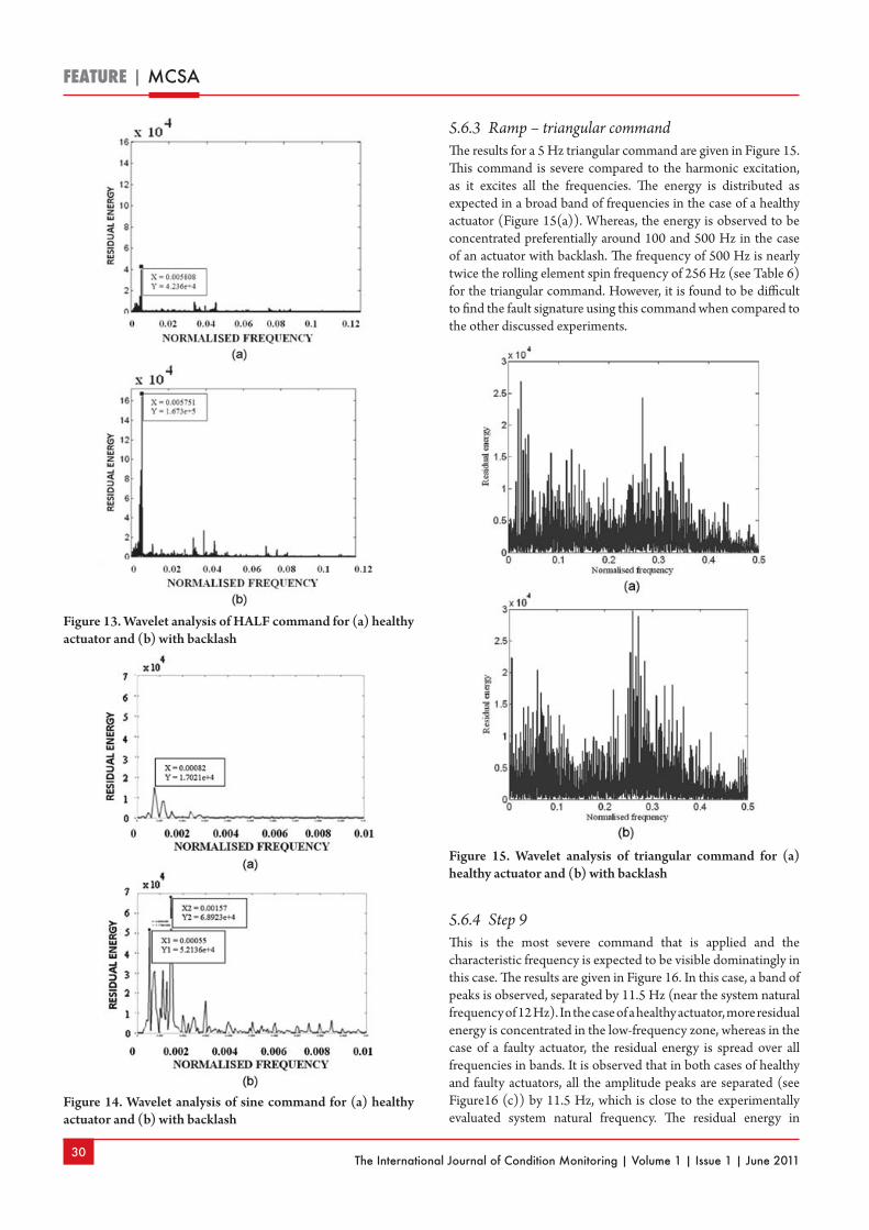
The International Journal of Condition Monitoring | Volume 1 | Issue 1 | June 201130
FEATURE | MCSA
5.6.3 Ramp – triangular commandThe results for a 5 Hz triangular command are given in Figure 15. This command is severe compared to the harmonic excitation, as it excites all the frequencies. The energy is distributed as expected in a broad band of frequencies in the case of a healthy actuator (Figure 15(a)). Whereas, the energy is observed to be concentrated preferentially around 100 and 500 Hz in the case of an actuator with backlash. The frequency of 500 Hz is nearly twice the rolling element spin frequency of 256 Hz (see Table 6) for the triangular command. However, it is found to be difficult to find the fault signature using this command when compared to the other discussed experiments.
5.6.4 Step 9 This is the most severe command that is applied and the characteristic frequency is expected to be visible dominatingly in this case. The results are given in Figure 16. In this case, a band of peaks is observed, separated by 11.5 Hz (near the system natural frequency of 12 Hz). In the case of a healthy actuator, more residual energy is concentrated in the low-frequency zone, whereas in the case of a faulty actuator, the residual energy is spread over all frequencies in bands. It is observed that in both cases of healthy and faulty actuators, all the amplitude peaks are separated (see Figure16 (c)) by 11.5 Hz, which is close to the experimentally evaluated system natural frequency. The residual energy in
Figure 15. Wavelet analysis of triangular command for (a) healthy actuator and (b) with backlash
Figure 13. Wavelet analysis of HALF command for (a) healthy actuator and (b) with backlash
Figure 14. Wavelet analysis of sine command for (a) healthy actuator and (b) with backlash

The International Journal of Condition Monitoring | Volume 1 | Issue 1 | June 201131
MCSA | FEATURE
the case of the healthy actuator is concentrated at and around 150 Hz and 475 Hz, which is in close match with the rolling element spin frequency of 493 Hz (see Table 6) for the step 9 V command.
In the case of backlash, peaks corresponding to 493 Hz have increased significantly. However, it is relatively difficult to find the signature of a backlash fault using the step response test owing to the fact that a large number of peaks are present in the residual spectrum.
5.6.5 Summary of backlashFrom all the discussions in Sections 5.6.1 to 5.6.4, the effect of the backlash is observed to be an overall increase of residual energy. The backlash fault shifts the residual energy to higher frequencies, but spread over all frequencies in bands. The backlash is clearly detectable in the low-frequency HALF command with
a considerable increase of peak at the system natural frequency of 11.5 Hz, making it alone sufficient for detection. In the case of the sine command, the fault is detectable with the increase in amplitude at the exciting frequency and rolling element spin frequency. In the case of the other two tests, it is detectable, but comparatively difficult due to the fault signature peaks submerged in the large number of peaks.
6. ConclusionsIt is observed that, in comparison with vibration, MCSA is simple in terms of both experimentation and data analysis. In the case of broken gear tooth faults, the vibration signatures are sensitive to the amplitude of peaks at GMF and rotor running harmonics. In the case of MCSA, the signatures (peaks at GMF harmonics) are also sensitive to pattern change, in addition to the amplitude, thus making fault detection much easier. The sidebands corresponding to gear mesh frequency are directly visible in the FFT of MCSA without requiring further analysis such as cepstrum, which is required in the case of vibration signatures.
Unlike the previous studies, in the present study there are closed-loop feedback systems and hence the error corrections; also, the control loop tries to correct the errors and thus affects the system dynamics. The effect of loads below the operating load on the MCSA fault signatures is observed to be very small compared to vibration signatures.
The improper preload is difficult to detect using MCSA compared to the vibration technique. However, for all other faults experimented, MCSA outperformed the vibration technique. The high-amplitude low-frequency (HALF) command covering the entire range of transmission elements very slowly is found to be the best suited for fault detection. The present experimental study envisages a great utility and is a step towards building a diagnosis model of typical faults.
Appendix – AFFT and wavelet calculations are done through the Matlab (R2008b) of M/s Mathworks Inc software.
FFT analysis:%%%%%%%%%%%%%DATA ENTRY for current%%%%%%%%%%%%%%%%%%%%%%% clear all% close all% clc% name=’FREQ.csv’ %%ENTER THE FILE NAME HERE% sree = importdata(name, ‘,’, 16);%CHECK HEADER LINES% cur=sree.data(:,4);%%%%%CHECK APPROPRIATE DATA% cur=cur’;% plot(cur)% [x,y]= ginput(2);% cur=cur(floor(x(1)):ceil(x(2)));% plot(cur)% clear(‘sree’,’x’,’y’)
%%%%%%%%%%%%DATA ENTRY for vibration%%%%%%%%%%%%%%%%%%%%%%clear allclose allclcname=’half.mat’ ;%%ENTER THE FILE NAME HEREsree = importdata(name);cur=sree.Data1_R1____;plot(cur)[x,y]= ginput(2);cur=cur(floor(x(1)):ceil(x(2)));
Figure 16. Wavelet analysis of step 9 V command for (a) healthy actuator, (b) with backlash and (c) zoomed plot of part of (b)
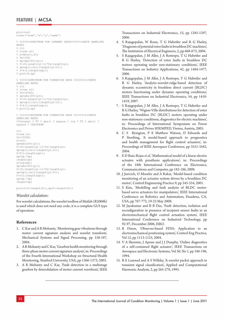
The International Journal of Condition Monitoring | Volume 1 | Issue 1 | June 201132
FEATURE | MCSA
plot(cur)clear(‘sree’,’x’,’y’,’name’)
% %%%%%%%SPECTRUM FOR CURRENT DATA%%%%%%(CHECK SAMPLING RATE)% clc% close all% y=data(:,4);% fs=100;% sp=abs(fft(y));% f=(0:length(y)-1)*fs/length(y);% sp=sp(1:ceil(length(y)/2));% f=f(1:length(sp));% plot(f,sp)
% %%%%%%SPECTRUM FOR VIBRATION DATA %%%%%%%%(CHECK SAMPLING RATE)% clc% close all% fs=10240;% sp=abs(fft(y));% f=(0:length(y)-1)*fs/length(y);% sp=sp(1:ceil(length(y)/2));% f=f(1:length(sp));% plot(f,sp)
% %%%%%%CEPSTRUM FOR VIBRATION DATA %%%%%%%%(CHECK SAMPLING RATE)%%%signal ? FT ? abs() ? square ? log ? FT ? abs() ? square ? CEPSTRUM
clcclose allfs=10240;y=cur;sp=abs(fft(y));f=(0:length(y)-1)*fs/length(y);sp=sp(1:ceil(length(y)/2));f=f(1:length(sp));sp=sp.*sp;length(sp)y=log(sp);sp=abs(fft(y));f=(0:length(y)-1)*fs/length(y);sp=sp(1:ceil(length(y)/2));f=f(1:length(sp));sp=sp.*sp;length(sp)
plot(f(5:length(f)),sp(5:length(f)))
Wavelet calculation:For wavelet calculations, the wavelet toolbox of Matlab (R2008b) is used which does not need any code; it is a complete GUI type of operation.
References1. C Kar and A R Mohanty, ‘Monitoring gear vibrations through
motor current signature analysis and wavelet transform’, Mechanical Systems and Signal Processing, pp 158-187, 2004.
2. A R Mohanty and C Kar, ‘Gearbox health monitoring through three-phase motor current signature analysis’, in: Proceedings of the Fourth International Workshop on Structural Health Monitoring, Stanford University, USA, pp 1366-1373, 2003.
3. A R Mohanty and C Kar, ‘Fault detection in a multistage gearbox by demodulation of motor current waveform’, IEEE
Transactions on Industrial Electronics, 53, pp 1285-1297, 2006.
4. S Rajagopalan, W Roux, T G Habetler and R G Harley, ‘Diagnosis of potential rotor faults in brushless DC machines’, The Institution of Electrical Engineers, 2, pp 668-673, 2004.
5. S Rajagopalan, J M Aller, J A Restrepo, T G Habetler and R G Harley, ‘Detection of rotor faults in brushless DC motors operating under non-stationary conditions’, IEEE Transactions on Industry Applications, 42, pp 1464-1477, 2006.
6. S Rajagopalan, J M Aller, J A Restrepo, T G Habetler and R G Harley, ‘Analytic-wavelet-ridge-based detection of dynamic eccentricity in brushless direct current (BLDC) motors functioning under dynamic operating conditions’, IEEE Transactions on Industrial Electronics, 54, pp 1410-1419, 2007.
7. S Rajagopalan, J M Aller, J A Restrepo, T G Habetler and R G Harley, ‘Wigner-Ville distributions for detection of rotor faults in brushless DC (BLDC) motors operating under non-stationary conditions, diagnostics for electric machines’, in: Proceedings of International Symposium on Power Electronics and Drives SDEMPED, Vienna, Austria, 2005.
8. C S Byington, P E Matthew Watson, D Edwards and P Stoelting, ‘A model-based approach to prognostics and health management for flight control actuators’, in: Proceedings of IEEE Aerospace Conference, pp 3551-3562, 2004.
9. E D Ruiz-Rojas et al, ‘Mathematical model of a linear electric actuator with prosthesis applications’, in: Proceedings of the 18th International Conference on Electronics, Communications and Computer, pp 182-186, 2008.
10. J Juricich, O Moseler and A Rakar, ‘Model-based condition monitoring of an actuator system driven by a brushless DC motor’, Control Engineering Practice 9, pp 545-554, 2001.
11. S Kim, ‘Modelling and fault analysis of BLDC motor-based servo actuators for manipulators’, IEEE International Conference on Robotics and Automation, Pasadena, CA, USA, pp 767-772, 19-23 May 2008.
12. M Jayakumar and B B Das, ‘Fault detection, isolation and reconfiguration in presence of incipient sensor faults in an electromechanical flight control actuation system’, IEEE International Conference on Industrial Technology, pp 92-97, December 2006, ISRO.
13. R Dixon, ‘Observer-based FDIA: Application to an electromechanical positioning system’, Control Eng Practice, Vol 12, pp 1113-1125, 2004.
14. V A Skormin, J Apone and J J Dunphy, ‘Online diagnostics of a self-contained flight actuator’, IEEE Transactions on Aerospace and Electronic Systems, Vol 30, No 1, pp 186-196, 1994.
15. R E Learned and A S Willsky, ‘A wavelet packet approach to transient signal classification’, Applied and Computational Harmonic Analysis, 2, pp 265-278, 1995.

The International Journal of Condition Monitoring | Volume 1 | Issue 1 | June 201133
FAULT DIAGNOSIS | FEATURE
The technique of machinery condition monitoring has been greatly enhanced over recent years with the application of many effective classifiers. However, these classification methods suffer from the ‘curse of dimensionality’ when applied to high-dimensional condition monitoring data. Actually, many classification algorithms are simply intractable when the number of features in the data is sufficiently large. In order to solve the problem, engineers have to resort to complicated feature extraction methods and other statistical theories to reduce the data dimensionality. However, features extracted using these methods lose their original engineering meaning and become obscure for engineers. In this study, a novel feature selection algorithm is presented to help to identify machinery condition quickly, based only on frequency spectrum data and without considering any complicated feature extraction methods. This brings many significant benefits: it can not only help engineers out of difficulties with complicated feature extraction methods, but it also gives a clear insight into the real condition of machinery without any loss of engineering meaning from the features used. The algorithm forms a functional extension of a relevance vector machine to feature selection, with a fast step-variable sequential backward search algorithm to search relevant scale parameters within a kernel function. Two case studies on different levels of condition monitoring are conducted to demonstrate the potential of applying the algorithm to high-dimensional engineering data.
Keywords: Feature selection, relevance vector machine, step-variable sequential backward search, fault diagnosis, condition monitoring.
1. IntroductionThe increasing complexity of modern machinery demands effective fault detection and diagnosis with low cost, high efficiency and reliability, and this in turn depends upon accurate pattern classification. Pattern classification methods can help to establish the relation between the measured symptoms and the
faults. The study to apply pattern classification to fault diagnosis has been greatly improved over recent years with the development of several classifiers, for example neural networks[1-4], support vector machine (SVM) and k-nearest neighbour (k-NN)[9] etc. However, the data used to represent a complex system is often high-dimensional with possibly hundreds and thousands of variables from a variety of sensors. Moreover, the number of samples is often limited due to the workload of data acquisition and processing, compared with large dimensions of the data. This makes pattern classification methods suffer from the ‘curse of dimensionality’. Many classification algorithms are intractable when the number of features in the data is sufficiently large. This problem is further exacerbated by the fact that many features in a learning task may either be irrelevant or redundant to other features with respect to predicting the class of an instance[10].
In order to solve the problem, engineers have to resort to spectra detection techniques[11] or feature extraction methods. Feature extraction methods as a dimensionality reduction technique are widely used in condition monitoring, for example principal component analysis (PCA)[12-14], high-order statistics (HOS)[15,16], independent component analysis (ICA)[17,18] etc. However, the choice and exploitation of all these methods demands a great knowledge of statistics and experience of engineering data processing. Besides, the new features transformed by feature extraction methods have usually lost the engineering meaning of the original features, which prevents engineers, used to visual inspection of frequency spectra, from understanding the essential correlation between features and machinery condition.
For this reason, other forms of dimensionality reduction technique – feature selection methods – are also applied in fault diagnosis, for example the distance measurement-based algorithm[19,20], sequential backward search (SBS)[21], decision tree analysis[6] etc. According to the survey on these feature selection methods, it is found that the candidate features for further selection are not high-dimensional ones based on the simple time-frequency spectrum, but a few statistical features extracted by using some complicated feature extraction methods or statistical theories. For example, the paper[6] attempts to select features from 11 statistical features such as mean, standard deviation and kurtosis using a decision tree. In the paper[19], the candidate features for selection are 24 independent components and principal components resulting from feature extraction processes such as ICA and PCA. This still requires pre-processing of complicated feature extraction and leads to a loss of the original meaning of features.
In this study, a novel feature selection method called RVM-StepSBS is presented. This method focuses on feature selection for high-dimensional data from the simple time-frequency
Kui Zhang is with Salford Business School, The University of Salford, Manchester M5 4WT, UK. Email: [email protected]
Andrew D Ball and Fengshou Gu are with the School of Computing & Engineering, The University of Huddersfield, Huddersfield HD1 3DH, UK. Email: [email protected]
Yuhua Li is with the School of Computing & Intelligent Systems, The University of Ulster, Londonderry BT48 7JL, UK.
A novel feature selection algorithm for high-dimensional condition monitoring dataKui Zhang, A D Ball, Yuhua Li and Fengshou Gu
Submitted 04.09.10 Accepted 10.02.11

The International Journal of Condition Monitoring | Volume 1 | Issue 1 | June 201134
FEATURE | FAULT DIAGNOSIS
spectrum and ignores the complicated feature extraction methods. Not only can it be readily understood by field engineers who are unfamiliar with statistical methods, but it can be applied to high-dimensional data processing. Another notable fact is that the method facilitates data visualisation and data understanding by discarding irrelevant features.
The relevance vector machine (RVM) is a statistical learning method in a Bayesian probabilistic learning framework. Since its introduction by Tipping in 2000[22], it has been successfully applied to a number of applications[23-27]. The key feature of this approach is that the inferred predictors are particularly sparse. The majority of weight parameters are automatically set to zero during the learning process[22], in deference to the principle of automatic relevance determination, which was originally formulated in the framework of Bayesian neural networks[28,29]. However, the RVM cannot compete with the support vector machine in terms of training time, although it can deliver many sparse models[30]. The computational cost with matrix inversion is challenging, especially when applied to high-dimensional data with redundant features. Therefore, feature selection becomes a potential topic to extend the RVM performance. Tipping suggests a way to deal with irrelevant input variables by tuning multiple input scale parameters within kernels, for example the width parameters of the Gaussian kernel. Tipping also attempts to realise it by using conjugate gradient methods, ie a joint non-linear optimisation over hyperparameters and scale parameters. However, he admits that the optimisation algorithm is computationally demanding, and it is impractical when applied to complicated high-dimensional data processing. This paper therefore explores a novel feature selection algorithm called RVM-StepSBS to select optimal features by applying a step-variable sequential backward search (StepSBS) algorithm to scale parameter selection within a kernel function, aiming at maintaining or improving the generalisation performance of the RVM.
The paper is organised into five main sections. Section 2 begins with an introduction to feature selection and then presents a novel step-variable sequential backward search algorithm (StepSBS) based on an analysis of the sequential backward search (SBS) algorithm. In Section 3, a structured analysis of the extended RVM for feature selection is given based on a parameter tuning theory within a kernel function. Section 4 offers further insight into how to apply the StepSBS algorithm to scale parameter selection in order to achieve the goal of feature selection with high accuracy in classifier performance. In order to demonstrate the advantages of the algorithm in processing high-dimensional condition monitoring data, two case studies are presented in Section 5. The final section contains a summary of the paper and a look towards future work.
2. Step-variable sequential backward search for feature selection
2.1 Feature selectionFeature extraction creates new features based on transformations or combinations of the original feature set[31], while feature selection chooses a set of features from existing features and does not construct new ones[32]. Feature selection is defined by many
authors by looking at it from various angles. In terms of space mapping, feature selection can be considered as a mapping from a high-dimensional space to a lower-dimensional feature space. The mapping should be carried out without severely reducing class separability[33]. When emphasising the reduction in the number of features, feature selection is to select a subset of d features from the given set of D measurements, d<D, without significantly degrading the performance of the recognition system[34]. In considering the improvement of prediction accuracy, the problem of feature selection is to select a subset of d features from a large set of D features or measurements to optimise the value of a criterion over all the subsets of the size d[35]. In this study, the main goal of feature selection is to seek the smallest subset of features without significantly degrading the performance of classification, ie to find the smallest subset of features for which the classification error rate is below a certain specified level.
Feature selection methods can be divided into three main types: filters, wrappers and embedded approaches. Filters select subsets of variables as a pre-processing step, independently of the chosen predictor[36]. Wrappers conduct a search for a good subset using the classification algorithm itself as part of the evaluation function[32]. In embedded methods, the feature selection is embedded within the classification algorithm[37]. Embedded methods perform variable selection in the process of training and are usually specific to given learning machines[36]. In this study, an embedded method for an RVM is employed to select features with the aim of keeping the error rate of classification below a threshold.
A feature selection method is usually based on two basic components: evaluation criterion and search procedure. The evaluation criterion must be defined to judge whether one subset of features is better than another[38]. Dash[39] divides the evaluation criterion into five categories: distance measures, information measures, dependence measures, consistency measures and classifier error rate measures. In this study, the classification error rate of the relevance vector classifier is chosen as the evaluation criterion. Also, a good systematic search procedure is very important when searching through the subsets of candidate features. The search strategies are categorised into three groups by Doak[40,41]: exponential search (for example exhaustive search, Branch and Bound[35]), randomised search (for example simulated annealing, probabilistic hill-climbing, genetic algorithms[42]) and sequential search (for example sequential backward search (SBS), sequential forward search (SFS), floating selection[34], plus l and take away r (PTA(l, r))). The exponential search is the most computationally complex approach which is impractical for problems with very large feature sets[34]. Although genetic algorithms are suitable for high-dimensional problems, the setting of parameters is difficult[43]. Therefore, a search algorithm called step-variable sequential backward search (StepSBS) is developed in this research, in search of the relevant scale parameters of the kernel function in the RVM to achieve the goal of feature selection.
2.2 Sequential backward search (SBS)The procedure of sequential backward search (SBS) is to start with the complete set Y of the dimensionality D, and to eliminate

The International Journal of Condition Monitoring | Volume 1 | Issue 1 | June 201135
FAULT DIAGNOSIS | FEATURE
one variable at a time. At each stage of the algorithm, the feature chosen for elimination is the one which keeps the value of the selection criterion below a given threshold with its removal. The algorithm is described in Table 1.
2.3 Step-variable sequential backward search (StepSBS)
The SBS algorithm is realised by removing one feature at one time. Since the data embodying important engineering information is often located in some particular region of the frequency domain rather than spread over the whole frequency range, irrelevant features can be removed piece by piece instead of one by one. Thus, a generalised step-variable sequential backward
search (StepSBS) algorithm has been developed in this study to speed up the search for significant features. In the algorithm, the input feature set is divided into several partitions and all of the features in any certain partition are removed at one time. For example, the bearing data reported in Section 5.1 is comprised of 200 frequency features. The 200 features can be grouped into 20 partitions, each including 10 features (referred to in this study as having a step length of 10). In the search process, 10 features are then eliminated at one time. Thus, in the first search, 200 iterations in the SBS decrease to 20 iterations in the StepSBS, which greatly improves the efficiency of the SBS.
Table 2 describes this algorithm in detail. In the StepSBS, the candidate feature set is usually divided into two partitions
at the beginning of the search. When the classification error rates are all beyond a given threshold with the removal of any partition, ie no irrelevant features are found, the candidate dataset will be divided into smaller partitions. When some irrelevant features are found and removed, the remaining feature subset is regarded as a new candidate feature set with which to start the next search. The search will stop when the step length becomes 1 and the performance of the classifier is beyond the threshold with removal of any feature.
3. Relevance vector machine for feature selection
Since the RVM was proposed by Tipping[22], it has faced a challenge from the processing of high-dimensional data, especially when the number of variables is larger than the number of total training instances. Thus, feature selection becomes an important topic in the RVM. This section will present an insight into how a standard algorithm of the RVM classifier, with single scale parameters within a Gaussian kernel, is extended to perform feature selection by employing multiple scale parameters within the kernel.
3.1 Standard RVM classifier modelThe sparse linear model RVM, like the support vector machine (SVM), performs a non-linear projection of a D-dimensional input space x∈RD into a high-dimensional (often infinite) feature space H by a set of non-linear basis functions[44].
Given an input set x = [x1,x2,…,xM]T with xm = [xm1,xm2,…,xmD] (D is the number of input variables or dimensions), the output function of the RVM classifier model is of the form:
Table 1. Sequential backward search algorithm
(1) Input: Y = {yi | i = 1,…,D}; /*complete set of measurements*/ Output: Xk = {xi | i = 1,…, k, xi ∈ Y}, k = 1,…,D; Evaluation function threshold: f0 ; /*set minimum error rate of classifier as evaluation
function */(2) Initialization: k :=D; X :=Y;(3) /* Start SBS*/ Repeat if f(Xk – x–) ≤ f0 /* find one nonsignificant feature x– in Xk */ then Xk–1
:= Xk – x–; /* remove one nonsignificant feature at a time */ Xk
:= Xk–1; k := k – 1; endif Stop when the performance of classifier will not be improved with the decrease of features;(4) Return Xk
Table 2. Step-variable sequential backward search algorithm
(1) Input: Y = {yi | i = 1,…,D}; /*complete set of measurements*/ Output: Xk = {xi | i = 1,…, k, xi ∈ Y}, k = 1,…,D; Evaluation function threshold: f0 ; /*set minimum error rate of classifier as evaluation
function */(2) Initialization: X := Y; k := D; q := 2;(3) /*Start StepSBS*/ Repeat s = D/q; /* set step length s, where q is the number of partitions*/ while (finishing testing all the partition of the features) X– = xi
– (i = 1,…,s) /* remove one partition of features with step length s */ if f(Xk – X–) ≤ f0 /* find one partition of nonsignificant features xi
– in Xk */ then Xk–s := Xk – X–; /*remove one partition of nonsignificant features at a time*/ Xk := Xk–s; k := k – s; endif (test next partition of features) endwhile if (k < D) D := k; /*there are features removed*/ else q := q + 1; endif Stop when the performance of classifier will not be improved by removing any feature with
s = 1; (4) Return Xk

The International Journal of Condition Monitoring | Volume 1 | Issue 1 | June 201136
FEATURE | FAULT DIAGNOSIS
y x( ) = wΤΦ(x, ′x ) = wn
n=1
N
∑ Φ(x, ′xn) .......................(1)
where ′x = ′x
1, ′x
2,…, ′x
N[ ]T is the training set with
′xn= ′x
n1, ′x
n2,…, ′x
nD[ ] .The supervised learning is to attempt to construct the classifier
function y that can map the training vector ′x = ′x
1, ′x
2,…, ′x
N[ ]T
onto the corresponding target t = t
1,t2,…, t
N[ ]T , ie to estimate
the weights w = w
1,w
2,…,w
N[ ]T . In the RVM scheme, the
estimated value of the model weights is given by the mean of the posterior distribution, which is also the maximum a posteriori (MP) estimation of the weights[44,45].
The basis function Φ x, ′x( ) is the M×N design matrix with Φ(x, ′x
n) = Φ x
1, ′x
n( ),Φ x2, ′x
n( ),...,Φ xM, ′x
n( ) Τ
. For the purpose of feature selection in this study, it is chosen as a Gaussian kernel centred on each of the training points:
Φ xm, ′x
n( ) = exp −1
r2xm− ′x
n
2
= exp −η x
md− ′x
nd( )2
d=1
D
∑
...(2)
where r is the input scale (or width) parameter and η =1
r2
.
The model introduces a prior over the model weights and assigns an individual hyperparameter αn (n = 1,2,…,N) to each weight wn or basis function. The zero-mean Gaussian prior distribution over w is:
p w α( ) = ∏n=1
N
Ν wn0,α
n
−1( ) = ∏n=1
N αn
2πexp −
αnwn
2
2
........(3)
According to the Bayesian theorem, the posterior probability of w is:
P w t,α( ) =P t w,α( ) p w α( )
p t α( ) ..........................(4)
where p(w|α) is a prior which can be calculated by (3), p(t|α) is the evidence and P(t|w,α) is the likelihood, which can be calculated by:
P t w,α( ) = ∏n=1
N
f yn( )tn1− f yn( )
1−tn
...............(5)
where f(y) = 1/(1+e–y) is the logistic sigmoid link function with yn = y(xn,w).
Since , P(w|t,α) ∝ P(t|w,α)p(w|α), the most probable weight wMP can be obtained by finding the maximum of:
log P w t,α( )( ) = tn log f yn( )( ) + 1− tn( ) log 1− f yn( )( ) −αnwn
2
2
n=1
N
∑ ..(6)
The quantity is differentiated twice to give:
∇w∇wlogP w t,α( ) w
MP
= − ΦΤ&Φ +A( ) ..............(7)
where B = diag{f(yn)[1–f(yn)]} and A = diag(α1,α2,…,αN).So, the covariance and mean for a Gaussian approximation to
the posterior around weight centred at wMP (in place of μ) can be obtained:
Σ = ΦTBΦ +A( )
−1
...................................(8)
µ = ΣΦTBt ..........................................(9)
Update αn by using[22,46]:
αn
new =1−α
n
oldΣn,n
µn
2 .....................................(10)
where Σn,n is the nth diagonal component of the posterior covariance given by (8) and μn is the nth component of the posterior mean given by (9).
If αn exceeds a preset maximum value, the corresponding weight wn is set to zero and the corresponding Φ is removed. After several iterations, just a few active terms in (1) are retained. The remaining active vectors with non-zero weights are called the relevance vectors. With the sparse vectors, the trained RVM can be used to classify the unseen data efficiently.
3.2 Extended RVM for feature selectionIt is worth pointing out that the width parameters η (or r) of the Gaussian kernel in the standard RVM model are set uniformly for all feature variables (See Equation (2)). As a matter of fact, the performance of the RVM heavily depends on the width parameters[44]. Tipping suggested that the use of the multiple input scale parameters within kernels can be an effective way of dealing with irrelevant input variables[22]. Following this suggestion, an adaptive Gaussian kernel Φ x
m, ′x
n( ) with multiple scale parameters is presented in this study:
Φ xm, ′x
n( ) = exp −1
rd
2xmd− ′x
nd( )2
d=1
D
∑
= exp − η
dxmd− ′x
nd( )2
d=1
D
∑
... (11)
Compared with Equation (2), it is found that width parameters ηd= r
d
−2d =1,2,...,D( ) are assigned to each of D input variables
individually, instead of a common width parameter being used. In the probabilistic interpretation, the kernel function is the prior covariance function. The width parameter ηd determines the distance between test data and training data in each feature direction d. As a width parameter becomes small, the Gaussian kernel becomes relatively insensitive to the corresponding input variable[46]. If the performance of classification will not significantly degrade when ignoring the input variable corresponding to a small width parameter, this indicates that the input variable is irrelevant for classification. Thus, a goal of feature selection can be achieved by selecting the width parameters within a Gaussian kernel.
Tipping attempts to estimate these width parameters by performing a cycle of maximisation of the marginal likelihood with respect to ηd (d = 1,2,…,D) at each iteration of the hyperparameter update, ie a joint non-linear optimisation over hyperparameters and scale parameters by using conjugate gradient methods. However, he admits that the optimisation algorithm is computationally demanding and it is impractical when applied to complicated high-dimensional data processing. Thus, the following idea for feature selection is proposed in this study:
When the error rate of the classification with ηd set to 0 is kept below a threshold, the corresponding dth feature is regarded as a non-significant feature for the performance of the classifier and can be removed. Conversely, when the error rate of the classification with ηd = 0 is greater than the threshold, the corresponding feature cannot be eliminated as it includes significant information for classification.

The International Journal of Condition Monitoring | Volume 1 | Issue 1 | June 201137
FAULT DIAGNOSIS | FEATURE
This idea forms a functional extension of a standard RVM classifier to feature selection. It can realise feature selection by using the StepSBS algorithm to search significant features based on the corresponding setting of scale (or width) parameters within a Gaussian kernel in the RVM. Since only the optimisation of weights and hyperparameters is emphasised during iterations, this idea delivers a practical solution for the processing of high-dimensional data.
4. Feature selection by applying StepSBS to parameter selection within the kernel of an RVM
This section details the proposed feature selection method which the authors have named the RVM-StepSBS. The method enables feature selection by applying the StepSBS algorithm to scale parameter selection within the kernel function of the RVM. The aim of this algorithm is to find the relevance of certain features to the performance of the classifier. If the accuracy of the classifier has not been affected significantly when the values of certain scale parameters are set to zero, the corresponding features are considered to be irrelevant features or weakly relevant features. Conversely, if the accuracy of the classifier decreases very greatly with some scale parameters set to zero, the corresponding features are considered to be strongly relevant and should be kept.
4.1 RVM-StepSBS algorithmWe can choose SBS as a search method for scale parameter selection, but it is an inefficient method with one feature being removed at one time. Instead of SBS, a generalised StepSBS algorithm has been developed in this study. This is a step length variable method used in the process of parameter search, but the step length is fixed within each search phase. RVM-StepSBS performs feature selection with a fast StepSBS algorithm to search relevant scale parameters within a kernel function. The procedure can be explained as follows:1. Input a training dataset and a test dataset with a known
classification target.2. Initialise all scale parameters ηd (d = 1,2,…,D) to some non-
zero initial value η0, where D is the dimension of the candidate feature set.
3. Set a minimum error rate f0 of the classifier as a threshold.4. Initialise the number of partitions (q) into which the candidate
feature set is divided, and divide the feature set accordingly. The choice of initial number of partitions depends on the problem to be solved (see Section 4.2), but q is usually initialised to 2 when the number of feature candidates is large.
5. Calculate the step length: s = D/q, and start to test the first partition of the feature set (i = 1). The step length is the number of features in a partition. If s = D/q is not an integer, then s will be rounded to the nearest integers greater than or equal to s. For example, in case study 1 in Section 5.1, when the candidate feature set including 200 features is divided into 3 partitions (D = 200 and q = 3), the step length is calculated as s = 67. The first two partitions include 67
features respectively, the remaining 66 features are included in the last partition.
6. Set the scale parameters of the ith partition of the feature set to zero: ηi = 0 (i = 1 + s * (i–1),…, s * i), and keep others unchanged (η0) in Gaussian kernel function for both training and test data, then calculate the classification error rate fi by using the relevance vector classifier.
7. If the error rate fi is greater than the minimum error rate f0 (fi > f0), ie the ith partition of the feature set is significantly relevant to the performance of the classifier, then the value of the corresponding ηi will be reset to η0. However, if the error rate fi is not greater than error rate f0 (fi ≤ f0), then the ith partition of the feature set is removed from both the training dataset and the test dataset. Go back to Step 6 to test the next partition of the feature set.
8. After finishing the search of q partitions via repeating Steps 6 and 7, assess if there are any features removed. If not, subdivide the feature set for further searching with q = q+1 and then go to Step 5. Otherwise, take the obtained feature subset as a new feature set with a new D and go back to Step 5.
9. Repeat Step 5 through to Step 8 until the classification performance cannot be below the threshold by setting any non-zero scale parameter to zero when s = 1.
4.2 Step lengthThe RVM-StepSBS is a flexible feature selection algorithm in which the step length can be changed freely, according to the problem to be solved and the number of features for selection. The following discussion identifies some special cases:n When the number of feature candidates is small (for example
D < 20) or the relevant features disperse or spread out from each other, the step length may be chosen as 1 (s = 1 or q = D). In this case, the StepSBS algorithm is just a standard SBS algorithm.
n When the number of feature candidates is large (for example D > 40) and the relevant features cluster together, the step length may be initialised as half the number of feature candidates, ie the feature candidates are divided into two partitions (q = 2). By comparison with the error rate of the classifier obtained from two partitions, it is easy to find which partition includes the more important information for classification. If the error rates of the two partitions are both far greater than the minimum error rate, ie relevant features exist on both sides, then the step length has to be much shorter, for example q = 3,4,…. After several iterations, the relevant feature partitions remain. The iteration will stop when the step length is 1.
n In some cases, the distribution of features shows some obvious periodicity, for example the line bearing defect data in Section 5.1. The step length may be chosen as a smaller value than the periodic length, for example by using an initial s = 10 rather than s = 100. The results obtained are similar, but the efficiency of the feature search is much higher than the case in which the search of step length starts with 100. This result is discussed in Section 5.3.

The International Journal of Condition Monitoring | Volume 1 | Issue 1 | June 201138
FEATURE | FAULT DIAGNOSIS
5. Application to high-dimensional condition monitoring data
Since data processing methods are evaluated based upon their usefulness in fault detection, diagnosis and severity assessment, the following two case studies deal with the topics of fault detection and severity assessment individually by using the RVM-StepSBS algorithm, and in this way the significance of the algorithm is demonstrated by its application to high-dimensional condition monitoring data.
5.1 Case Study 1: Severity assessment of faulty bearings
The failure of rolling element bearings is one of the major causes of breakdown of rotating machinery. The failure is likely to develop from fatigue cracks caused by cyclic contact stress. Detecting the onset of these defects and monitoring their development can often avoid catastrophic failures and economic loss. The following experiment was designed to investigate the correlation between frequency features of a monitored acoustic signal and the severity of defects in a bearing.
ExperimentIn this experiment, two different sizes of line defect were seeded on the outer race of bearings to simulate fatigue damage: a large defect (approximately 1.04 mm × 16 mm) and a small defect (approximately 0.11 mm × 6 mm). The data was acquired by an acoustic emission (AE) transducer placed directly on the bearing housing using equipment and procedures described previously[47], and then was converted into frequency spectrum data via envelope analysis.
Although it is straightforward for an experienced engineer to make a clear discrimination between the two faulty bearings based upon the characteristic frequency features of Figure 1, the visual inspection process depends on the skills of the engineer, familiarity with the bearing under investigation, the operating conditions and the signal analysis technique being used. Such intuitive judgement cannot meet the requirement of modern condition monitoring in terms of the discrimination accuracy and diagnosis efficiency.
Feature selection by the RVM-StepSBSThe feature selection by the RVM-StepSBS algorithm went through the following key phases:1. Dataset: 270 samples in 200 dimensions were obtained with
a known classification target. Each sample was composed of 200 elements, taken from the amplitude spectrum with a frequency resolution of 4.83 Hz, from 0 Hz to 1000 Hz. The sample dataset was split into a training set of 90 samples and a testing set of 180 samples.
2. Initialisation: Scale parameters were initialised to ηd = 4 (d = 1,2,…,200), and minimum error rate f0 = 5%.
3. Search: The candidates feature set was first split into two partitions (q = 2), so the length of step was calculated as s = D/q = 100. The calculation of the classification error rates was based on two sets of features: one with ηd = 0 (d = 1,2,…,100) and ηd = 4 (d = 101,102,…,200), and the other was opposite: ηd = 4 (d = 1,2,…,100) and ηd = 0 (d = 101,102,…,200). It was found that the error rates based on the two feature sets were both 46.67%, which means that there were relevant features in both partitions and hence the feature set should be divided into smaller partitions for further searching. When the feature set was divided into three partitions (q = 3 or s = 67), the error rates were 11.67%, 41.67% and 0.56%, respectively. The third error rate was less than the minimum error rate of 5% (0.56% < 5%), ie the last partition included less significant features. Thus, the features in the last partition were removed and only 134 features remained as a new feature set for further search. As shown in Figure 2, when s = 27, the number of features decreased from 134 to 108 with an error rate of 0.56% caused by the removal of 27 features. The number of features reached 92 when s = 11; 88 when s = 7; 74 when s = 6; 67 when s = 5; 62 when s = 4; 58 when s = 3; and 47 when s = 2. After the last iteration, when s = 1, only 6 features remained. The error rate of classification also decreased to 0, which was slightly lower than the original error rate (1.1%) based on the original feature set with ηd = 4.
4. Results: As a result, the selected features were: 18, 36, 53, 70, 87 and 104, which corresponded to frequencies of 86.94 Hz, 173.88 Hz, 255.99 Hz, 338.1 Hz, 420.21 Hz and 502.32 Hz.
Figure 1. AE envelope amplitude spectra of bearings with seeded defects
Figure 2. Step lengths, number of features and classification error rate (*0.05%) for bearing data

The International Journal of Condition Monitoring | Volume 1 | Issue 1 | June 201139
FAULT DIAGNOSIS | FEATURE
ValidationTo verify the selected features as the relevant features, a 2D visualisation of 270 bearing samples in Figure 3 is presented. In the sense of discrimination, it shows that two selected features (no 18 and no 36) are better than a randomly chosen pair of non-selected features (no 15 and no 20). The results demonstrate that the features selected by the RVM-StepSBS algorithm are significant for discrimination between data in two different classes. Also, this demonstrates another benefit of feature selection – to facilitate data visualisation and data understanding.
Engineering interpretationThe bearing type used in the investigation was an N406 parallel roller bearing of bore diameter 30 mm, outer diameter 90 mm, roller length 23 mm, pitch diameter 59 mm and having nine rollers of diameter 14 mm. Based on these geometric sizes and the rotational speed of 1,456 r/min (24.3 Hz), the outer-race defect frequency was easily calculated to be 83.3 Hz according to (12)[48]:
fo =Ne
2* fr 1−
BD
PDcosα
..........................(12)
where Ne is the number of elements, fr is the rotational frequency, BD is the roller diameter, PD is the pitch diameter and α is the contact angle (assumed to be zero since this is a parallel roller bearing).
If a fault produces a signal at a known frequency, then the magnitude of this signal is expected to increase as the fault develops. The seeded line defect on the outer race causes repetitive impulses when struck by the rollers and hence the defect should appear at that frequency, the values of which are multiples of 83.3 Hz. Obviously, the results obtained by using the RVM-StepSBS algorithm are comparable to the theoretical results, proving that in this case this algorithm has important engineering significance in revealing the correlation between the faults and relevant frequency features.
To demonstrate the significance of the developed algorithm, this section presented a simple example to help to understand the application process of this algorithm. The next section will show a demanding example in which the significant frequency features are not easily located by visual discrimination.
5.2 Case Study 2: Fault detection of induction motorAngular misalignment between the rotor and stator is a common cause of motor failure. It can cause excessive stress within the machine and greatly increase bearing wear. In addition, the radial magnetic force waves produced by misalignment can also act on the stator core and subject the stator windings to unnecessary and potentially harmful vibration. It is also feasible for a rotor-to-stator rub to occur with consequential damage to the windings and the rotor cage. This can lead to insulation failure of the stator windings or breaking of rotor cage bars or end-rings and hence require a costly repair[49]. Early and accurate fault detection and diagnosis are of key importance. The following experiment was conducted to examine the fault-related frequency domain features to distinguish angular misalignment of a faulty motor from a healthy motor, based on the vibration signature.
ExperimentIn this experiment, two 3 kW direct-on-line (DOL) three-phase induction motors were tested: a healthy motor and an angular misalignment faulty motor. The vibration data was collected by an accelerometer mounted vertically on the stator feet and then converted into frequency spectrum data (See Figure 4) by fast Fourier transformation (FFT). It is obvious that it is not easy to find discriminative features in Figure 4 via visual inspection, as was possible with the bearing case in Figure 1.
Feature selection by the RVM-StepSBSFeature selection with the RVM-StepSBS went through the following key phases:1. Dataset: 240 samples in 640 dimensions were taken from the
amplitude spectrum with a frequency resolution of 1.5625 Hz, from 0 Hz to 1000 Hz. The samples were split into two sets: a training set of 105 samples and a test set of 135 samples. Up to 640 features made it difficult for engineers to identify
Figure 3. Visualisation of the samples by selected features (a) and non-selected features (b)

The International Journal of Condition Monitoring | Volume 1 | Issue 1 | June 201140
FEATURE | FAULT DIAGNOSIS
the characteristic frequency features for fault diagnosis. 2. Initialisation: Scale parameters were set to ηd = 4
(d = 1,2,…,200), and minimum error rate f0 = 5%.3. Search: The search started with q = 2 (s = 340), ie the original
feature set was divided into two partitions. Since the error rates of classification calculated by separately setting one of the partitions ηd = 0 and the other ηd = 4 were all above a threshold of f0 (5%), the feature set had to be further subdivided. Until q = 4 (s = 160), the error rate of classification (4.44%) fell below a threshold of f0 (5%). Thus, the partition of features with ηd = 0 was removed, which made the number of features retained quickly decrease to 480, and a new feature set with 480 features was formed for further searching. Iteration stopped when the error rates of classification were all above the threshold, even though the step length was set to 1. (The process of the iteration is shown in Figure 5.)
4. Results: 22 features were selected which were mainly clustered around two frequency components. One was between 400 Hz and 423.44 Hz, and the other was between 900 Hz and 923.44 Hz.
ValidationTo add further confidence to the results obtained by the algorithm, another evaluation criterion called the Relief algorithm was applied to the same dataset. The Relief algorithm is a feature weight-based algorithm inspired by instance-based learning algorithms[50]. It samples instances randomly from the training set and updates the relevance weight values based on the Euclidean distance between the selected instance and the two nearest instances of the same and opposite class (the ‘near-hit’ and ‘near-miss’). ‘Near-hit’ is the instance having minimum Euclidean distance among all instances of the same class as that of the chosen instance; ‘near-miss’ is the instance having minimum Euclidean distance among all instances of a different class[39]. The weights of features are initialised to zero in the beginning, based on the intuitive idea that a feature is more relevant if it distinguishes between an instance and its ‘near-miss’ and less relevant if it distinguishes between an instance and its ‘near-hit’. After exhausting all instances in the sample, it chooses all features having weight greater than or equal to a threshold. As a result, the frequencies of the first six ranked features were mostly around 401.56 Hz or 900 Hz.
The results are obviously close to those obtained by the RVM-StepSBS algorithm. Therefore, the features selected by the RVM-StepSBS algorithm are very likely to be fault-related features.
Engineering interpretationIn this experiment, the seeded fault was that of angular misalignment between the rotor and stator, producing static eccentricity within the motor along the length of the air gap. It was seeded by insertion of eccentric steel rings into the drive end bearing housing, which enabled radial misalignment of 0.2 mm within the motor (having an initial air gap of 0.35 mm). Although the rotor could be spun freely by hand when radial misalignment of 0.2 mm was induced, the combined effects of unbalanced magnetic pull and in-operation deflected shape caused intermittent minor rotor-stator contact. This slight rubbing had the effect of redistributing the energy associated with the major frequency components into a range of mid-to-high frequencies (400-1000 Hz)[51].
The presence of static eccentricity can be detected by an accelerometer mounted vertically on the stator feet. The equation that can be used to predict the frequency components of interest is[52]:
fecc = fs kR± nd( )1− s( )p
± nw
........................(13)
where k is any integer (1,2,…), nw is the order of the stator time harmonics that are present in the power supply driving the motor (1, 3, 5,…), R is the number of rotor slots, p is the number of pole pairs, nd is the eccentricity order (nd = 0 for static eccentricity), fs is the fundamental supply frequency and s is the motor slip.
Here, the details of the induction motor tested are: number of rotor slots is 28, number of poles is 2, supply frequency is 50 Hz and slip at 75% load is 0.036. By inserting the parameter values into Equation (13), the eccentricity frequency components of 399.6 Hz and 899.6 Hz can be gained. Obviously, this theoretical result is consistent with the result obtained by the RVM-StepSBS algorithm despite a slight difference between the two.
Figure 4. Motor vibration spectra for healthy and faulty conditions
Figure 5. Step lengths, number of features and classification error rate (*0.05%) for motor data

The International Journal of Condition Monitoring | Volume 1 | Issue 1 | June 201141
FAULT DIAGNOSIS | FEATURE
5.3 Further experiment on choice of step length and scale parameters
Choice of step lengthIn terms of choice of step length, another two experiments with the same set of data from the bearing case were conducted (See Table 3).
Table 3. Comparison of the same dataset with different starting step length
Initial step length (s) 100 10 1
Initial number of partitions (q) 2 20 200
Total iterations 10 5 1
Original features 200 200 200
Selected features 6 7 7
Selected feature codes
18, 36, 53, 70, 87, 104
18, 36, 52, 70, 86, 87, 104
18, 36, 52, 53, 70, 87, 104
Error rate of classification with selected features
0 0 0
When the step length is initialised to 10 (q = 20) instead of 100 (q = 2) for the first iteration, 80 features are removed and the number of features decreases to 120 from 200. Then there is a reduction to 96 with s = 6, to 72 with s = 4 and to 27 with s = 3; finally there are seven features remaining: 18, 36, 52, 70, 86, 87 and 104. The result is surprisingly similar to the case starting with s = 100, but the iterations are far smaller. The choice of step length can often speed up the efficiency of feature selection, which depends upon the problem to be solved.
When the initial step length is chosen as 1, ie selecting feature using the SBS algorithm, it is found that the accuracy of feature selection is comparable to the results using the StepSBS algorithm. The SBS is obviously lower than the StepSBS in computational efficiency when applied to the data whose characteristic frequency features are concentrated in a certain frequency range. However, it is not lower than the StepSBS when the relevant features are scattered over a wide frequency range.
Choice of scale parametersTo disclose the effect of the non-zero scale parameters within a Gaussian kernel on the results of feature selection, an experiment was carried out on the dataset from the motor case, which includes 640 candidate features (See Table 4).
Table 4. Feature selection results with different scale parameters within Gaussian kernel
Scale parameters 1 2 3 4 5 6 7 8
Number of selected features
233 96 64 22 54 72 45 65
When the scale parameters are very small, for example when ηd = 1, 233 out of 640 features are selected as significant features. This means that plenty of irrelevant features in the remaining 233 features failed to be detected. In the RVM-StepSBS algorithm, the scale parameters are set to 0 when used to test whether the corresponding features are irrelevant. When ηd is very small, the features with the small ηd cannot be readily differentiated from the tested features with ηd = 0. The Gaussian kernel also becomes very insensitive to the features with small scale parameters.
However, nearly 90% of irrelevant features are removed successfully when scale parameters are chosen in the range between 3 and 8. In this motor case, ηd is chosen as 4, which delivers the smallest relevant feature set (only 22 features).
In summary, the RVM-SepSBS algorithm greatly depends on the choice of scale parameters and the improper choice of scale parameters can lead to failure of feature selection.
5.4 DiscussionsAs shown in Table 5, the processed data in the above-mentioned two cases are from different data sources and different test-rigs, and they are simply frequency spectrum data. The number of components (ie the number of features) is much greater than the number of acquired samples, which can readily cause problems with the generalisation performance of a classifier. With the use of the RVM-StepSBS algorithm, features related to the accuracy of classification are selected. The selected features account for only 3% of the original candidate features in the case of the bearing, and 3.4% in the case of the motor. Although the number of selected features is small, there exists significant engineering information in them. This information can help engineers to focus on the more important frequency components, to identify typical faults and make rapid decisions. Moreover, the accuracy of classification does not decrease with the removal of features; on the contrary, it improves, especially in the case of the motor.
Table 5. Comparison of two cases
Test-rig Bearing Induction motor
Sensor Acoustic emission transducer
Accelerometer
Training data 90 105
Test data 180 135
Original features 200 640
Selected features 6 22
Error rate of classification with whole features
1.11% 48.89%
Error rate of classification with selected features
0 2.22%
6. ConclusionsAlthough Tipping proposed the idea of dealing with irrelevant input variables by the use of the multiple input scale parameters within Gaussian kernels, his attempt on the estimation of these

The International Journal of Condition Monitoring | Volume 1 | Issue 1 | June 201142
FEATURE | FAULT DIAGNOSIS
width parameters by performing a joint non-linear optimisation over hyperparameters and scale parameters is proven to be impractical when applied to complicated high-dimensional data processing. The RVM-StepSBS algorithm solves the problem. It fixes the setting of scale parameters during iterations of hyperparameters, which allows the RVM to focus on the optimisation over hyperparameters and weights. Meanwhile, it uses the StepSBS algorithm to search relevant features based on the corresponding setting of scale parameters. The StepSBS algorithm is a flexible search strategy, because its step length can be changed according to the problem to be solved and the number of features for selection.
Furthermore, the RVM-StepSBS algorithm is proven to be practical in engineering applications where the relevant features come from some characteristic region of the frequency domain rather than being scattered over a wide frequency range. For instance, the discriminative frequency features in the bearing case are concentrated in the low frequency range, whilst the fault-related frequency features in the motor case are in the mid- to high-frequency range. The algorithm can remove the irrelevant features piece by piece and swiftly focus on the characteristic frequencies, which facilitates fault detection and diagnosis. Also, for the case in which the significant features are periodical, for example the bearing case, the efficiency of discrimination can further be improved by adjustment of the step length. However, it is not an efficient algorithm when fault-related features scatter over a wide frequency range or does not display periodical distribution. The choice of optimal step length is an intractable task. Moreover, when the frequency features are dynamic rather than static in real-time condition monitoring, the algorithm needs further exploration.
References1. W Lai et al, ‘Classification of gear faults using cumulants and
the radial basis function network’, Mechanical Systems and Signal Processing, 18, pp 381-389, 2004.
2. Y Li, M J Pont and N B Jones, ‘Improving the performance of radial basis function classifiers in condition monitoring and fault diagnosis applications where ‘unknown’ faults may occur’, Pattern Recognition Letters, 23, pp 569-577, 2002.
3. C T Kowalski and T Orlowska-Kowalska, ‘Neural networks application for induction motor faults diagnosis’, Mathematics and Computers in Simulation, 63, pp 435-448, 2003.
4. B Samanta, K R Al-Balushi and S A Al-Araimi, ‘Artificial neural networks and support vector machines with genetic algorithm for bearing fault detection’, Engineering Application of Artificial Intelligence, 16, pp 657-665, 2003.
5. S Yuan and F Chu, ‘Fault diagnosis based on particle swarm optimisation and support vector machines’, Mechanical Systems and Signal Processing, 2006.
6. V Sugumaran, V Muralidharan and K I Ramachandran, ‘Feature selection using decision tree and classification through proximal support vector machine for fault diagnosis of roller bearing’, Mechinical Systems and Signal Processing, 2006.
7. S Poyhonen et al, ‘Coupling pairwise support vector machines for fault classification’, Control Engineering Practice, 13, pp
759-769, 2005.8. V Sugumaran, G R Sabareesh and K I Ramachandran,
‘Fault diagnostics of roller bearing using kernel-based neighbourhood score multi-class support vector machine’, Expert Systems with Applications, 34, pp 3090-3098, 2008.
9. C K Mechefske and J Mathew, ‘Fault detection and diagnosis in low-speed rolling element bearings Part II: The use of nearest neighbour classification’, Mechanical Systems and Signal Processing, 6 (4), pp 309-316, 1992.
10. D Koller and M Sahami, ‘Towards optimal feature selection’, in Proceedings of International Conference on Machine Learning, 1996.
11. D A Clifton and L Tarassenko, ‘Novelty detection in jet engine vibration spectra’, in: The Sixth International Conference on Condition Monitoring and Machinery Failure Prevention Technologies, Dublin, Ireland, 2009.
12. N Baydar et al, ‘Detection of incipient tooth defect in helical gears using multivariate statistics’, Journal of Mechanical Systems and Signal Processing, 15 (2), pp 303-321, 2001.
13. Q He, F Kong and R Yan, ‘Subspace-based gearbox condition monitoring by kernel principal component analysis’, Mechanical Systems and Signal Processing, 21, pp 1755-1772, 2007.
14. I Trendafilova, ‘An automated procedure for detection and identification of ball bearing damage using multivariate statistics and pattern recognition’, Mechanical Systems and Signal Processing, 24, pp 1858-1869, 2010.
15. F Hernandez et al, ‘Application of higher-order statistics on rolling element bearings diagnosis’, in: Innovative Algorithms and Techniques in Automation, Industrial Electronics and Telecommunications, T Sobh et al editors, Springer, pp 145-148, 2007.
16. W Li, ‘A study of diesel engine acoustic characteristics’, University of Manchester, 2000.
17. W Li et al, ‘A study of the noise from diesel engines using independent component analysis’, Mechanical Systems and Signal Processing, 15 (6), pp 1165-1184, 2001.
18. Z Li et al, ‘Fault recognition method for speed-up and speed-down process of rotating machinery based on independent component analysis and factorial hidden Markov model’, Journal of Sound and Vibration, 291, pp 60-71, 2006.
19. A Widodo, B-S Yang and T Han, ‘Combination of independent component analysis and support vector machines for intelligent faults diagnosis of induction motors’, Expert Systems with Application, 2006.
20. K C Varghese, J H Williams and D R Towill, ‘Computer-aided feature selection for enhanced analogue system fault location’, Pattern Recognition, 10, pp 265-280, 1978.
21. R Casimir et al, ‘The use of feature selection and nearest neighbours rule for faults diagnostic in induction motors’, Engineering Application of Artificial Intelligence, 19, pp 169-177, 2006.
22. M E Tipping, ‘Sparse Bayesian learning and the relevance vector machine’, Journal of Machine Learning Research, 1, pp 211-244, 2001.
23. A Agarwal and B Triggs, ‘3D human pose from silhouettes by relevance vector regression’, Proceedings of the 2004 IEEE

The International Journal of Condition Monitoring | Volume 1 | Issue 1 | June 201143
FAULT DIAGNOSIS | FEATURE
Computer Society Conference on Computer Vision and Pattern Recognition, 2, pp 11882-11888, 2004.
24. A B Oliver Williams and R Cipolla, ‘Sparse Bayesian learning for efficient visual tracking’, IEEE Transaction on Pattern Analysis and Machine Intelligence, 27 (8), pp 1292-1304, 2005.
25. S Chen, S R Gunn and C J Harris, ‘The relevance vector machine technique for channel equalisation application’, IEEE Transactions on Neural Networks, 12 (6), pp 1529-1532, 2001.
26. Y Y Liyang Wei, R M Nishikawa and Yulei Jiang, ‘A study on several machine-learning methods for classification of malignant and benign clustered microcalcifications’, IEEE Transactions on Medical Imaging, 24 (3), pp 371-380, 2005.
27. J X Tao Yang, ‘The study of an improved relevance vector machine MUD based on perfect sampling’, Chinese Journal of Electronics, 13 (3), 2004.
28. D J C Mackay, ‘Bayesian methods for backpropagation networks in models of neural networks’, E Domany, J L v Hemmen and K Schulten editors, Springer, pp 211-254, 1994.
29. R M Neal, Bayesian Learning for Neural Networks, Springer, 1996.
30. Z Yang, ‘A fast algorithm for relevance vector machine’, Lecture Notes in Computer Science, 4224, pp 33-39, 2006.
31. D Z Anil Jain, ‘Feature selection: evaluation, application and small sample performance’, IEEE Transactions on Pattern Analysis and Machine Intelligence, 19 (2), pp 153-158, 1997.
32. R Kohavi and G H John, ‘Wrappers for feature subset selection’, Artificial Intelligence, 97 (1-2), pp 273-324, 1997.
33. K Fukunaga, Introduction to Statistical Pattern Recognition, Academic Press Limited, San Diego, CA, 1990.
34. J N P Pudil and J Kittler, ‘Floating search methods in feature selection’, Pattern Recognition Letters, 15, pp 1119-1125, 1994.
35. P M Narendra and K Fukunaga, ‘A branch and bound algorithm for feature subset selection’, IEEE Transactions on Computers, C-26 (9), pp 917-922, 1977.
36. I Guyon and A Elisseeff, ‘An introduction to variable and feature selection’, Journal of Machine Learning Research, 3, pp 1157-1182, 2003.
37. E Yom-Tov, ‘An introduction to pattern classification’, in: Advanced Lectures on Machine Learning, O Bousquet, U v Luxburg and G Ratsch editors, Springer, 2004.
38. C M Bishop, Neural Networks for Pattern Recognition,
Oxford University Press, 1997.39. M Dash and H Liu, ‘Feature selection for classification’,
Intelligent Data Analysis, 1, pp 131-156, 1997. 40. J Doak, ‘Intrusion detection: the application of input
selection, a comparison of algorithm, and the application of a wide area network analyser’, University of California, 1992.
41. I B T Ozge Uncu, ‘A novel feature selection approach: combining feature wrappers and filters’, Information Sciences, 2006.
42. M Srinivas, ‘Genetic algorithms: a survey’, Computer, pp 17-26, 1994.
43. M Kudo and J Sklansky, ‘Comparison of algorithms that select features for pattern classifiers’, Pattern Recognition, 33 (1), pp 25-41, 2000.
44. J Quinonero-Candela and L K Hansen, ‘Time series prediction based on the relevance vector machine with adaptive kernels’, in IEEE International Conference on Acoustics, Speech and Signal Processing, Orlando, USA, 2002.
45. C M Bishop and M E Tipping, ‘Bayesian regression and classification’, in: Advances in Learning Theory: Methods, Models and Applications, J A K Suykens, G Horvath and S Basu editors, IOS Press, pp 1-19, 2003.
46. C M Bishop, Pattern Recognition and Machine Learning, Springer, New York, 2006.
47. Y L Kui Zhang, Yibo Fan, Fengshou Gu and Andrew Ball, ‘An evaluation of the potential offered by a relevance vector classifier in machinery fault diagnosis’, International Journal of COMADEM, 9 (4), pp 35-40, 2006.
48. I M Howard, ‘A review of rolling element bearing vibration ‘detection, diagnosis and prognosis’’, DSTO Research Report 0013, 1994.
49. D G Dorrell and S Roach, ‘Analysis of airgap flux, current and vibration signals as a function of the combination of static and dynamic airgap eccentricity in three-phase induction motors’, IEEE Transactions on Industry Applications, 33 (1), pp 24-34, 1997.
50. D W Aha and M K Albert, ‘Instance-based learning algorithms’, Machine Learning, 6, pp 37-66, 1991.
51. B S Payne, ‘Condition monitoring of electric motors for improved asset management’, in: Manchester School of Engineering, University of Manchester, Manchester, UK, 2003.
52. M Arkan and M E Tagluk, ‘Bearing and misalignment fault detection in induction motors by using the space vector angular fluctuation signal’, Electrical Engineering, 87, pp 197-206, 2005.

Published by The British Institute of Non-Destructive Testing, Newton Building, St George’s Avenue, Northampton NN2 6JB, UK.
Tel: +44 (0)1604 89 3811; Fax: +44 (0)1604 89 3861; Email: [email protected]
www.bindt.org


![CONDITION MONITORING AND ASSESSMENT OF … Sankar May 13.pdf · Duval’s triangle [15] The triangle representation of fault diagnosis is shown in Fig.1.The three sides of the triangle](https://img.dokumen.tips/doc/110x75/5ab174c97f8b9abc2f8cb66f/condition-monitoring-and-assessment-of-sankar-may-13pdfduvals-triangle-15.jpg)