Monitoring infrastructure asset through its acoustic signature

Fedele, Rosario1

University Mediterranea of Reggio Calabria

Via Graziella, 89124, Reggio Calabria (RC), Italy

Praticò, Filippo Giammaria2

University Mediterranea of Reggio Calabria

Via Graziella, 89124, Reggio Calabria (RC), Italy

ABSTRACT

Structural health monitoring can benefit transportation infrastructures in terms of

pavement management systems and risk management. In this study, a new, non-

destructive, acoustic-based method for assessing and monitoring the structural

health status (SHS) of road pavements along their operational life is presented. In

order to validate the proposed method, an experimental investigation was carried

out. The acoustic response of an asphalt concrete road pavement following a proper

mechanical excitation (hereafter named acoustic signature) was recorded and

analysed. A specifically designed microphone-based electronic system was set up

and applied. The acoustic responses were analysed in the time and frequency

domain. An integrated system, including the power supply, the abovementioned

system, and data transmission equipment was set up and applied as a part of a

research project, to collect data and extract features and information valuable to

different stakeholders. Experimental results show that the proposed system is able

to detect the change of the acoustic signature of the infrastructure asset over time

using a small number of meaningful features extracted by clustering techniques.

Consequently, it can be used to monitor the SHS of road pavements by detecting the

onset of cracks, and keeping under observation their evolution over time.

Keywords: Acoustic signature, intelligent structural health monitoring, feature-based

hierarchical clustering

I-INCE Classification of Subject Number: 74

http://i-ince.org/files/data/classification.pdf

1. INTRODUCTION During its life time, a road pavement is subjected to repeated thermal and vehicular

traffic loads. These loads induce stresses, strains, displacements, and vibrations into the

pavement layers. These effects lead to the generation and propagation of several types of

cracks until the failure of the road pavement occurs. Many methods have been proposed

in the last decades in order to carry out the assessment and monitoring of the structural

conditions of road infrastructures in real conditions (e.g., under traffic-related stresses),

1 rosario.fedele@unirc.it 2 filippo.pratico@unirc.it

or under simulated stresses. Importantly, different factors should be taken into account

when road pavements need to be monitored. These factors mainly refer to: i) the sources

of the above-mentioned stresses, which in turn are function of vehicle-, and traffic-related

features [1]; ii) the mean of propagation of traffic-induced stresses (i.e., the pavement)

and its properties, performance, and conditions [2–6].

Road pavement Structural Health Monitoring (SHM) usually aims at detecting surface

cracks and rarely internal cracks. Tests and particularly Non-Destructive Tests (NDT) use

different types of sensors([7]), vehicles equipped with cameras [8], laser scanners [8,9],

vehicles equipped with three-axis accelerometers [10], with smartphone gyroscopes [11–

13], or accelerometers embedded or placed on the road surface [14,15]. Internal cracks

can be monitored using Ground Penetrating Radars (GPR; see e.g., [16]).

Intelligent solutions should be able to detect, in real-time, changes of the response of

a monitored road pavement to stresses and loads. To this end, a SHM system may need

to: i) identify variations of the signals collected; ii) recognize signals variations over time;

iii) derive the frequency components corresponding to the variations above; iv) detect the

“development” of new frequencies in the signals due to changes in the structural dynamics

[17]. In the last decades, different Intelligent Transportation System (ITS)-based and/or

SHM-based systems, with different data processing methods have been proposed, among

which filter-based methods [18], Gabor filter [19], Artificial Neural Network (ANN; cf.

e.g., [20,21], Wavelet Transform (WT) [17,22,23], or ANN combined with WT [9,12,24–

26]. Despite the high number of methods proposed, solutions are still needed to promptly

detect “invisible” (bottom-up) structural failures, which are crucial for flexible pavements

[27].

Based on preliminary studies [28,29], the study presented in this paper aims at solving

some of the issues listed above (see Section 2). Section 3 deals with the description of

method and experimental set-up. Section 4 deals with the results and is followed by

Conclusions.

2. OBJECTIVES

Based on previous section, the main objectives of this study are:

1) to present an innovative SHM method, specially designed for road pavements,

which is based on signal analysis.

2) to carry out a prototypical validation of the method, dealing with controlled

impulses.

3. METHOD AND EXPERIMENTAL SET UP

In this study, a cheap, simple, and NDT method for detecting underneath cracks and

allowing an intelligent road monitoring is presented. This method (see Figure 1) is

innovative and considers: 1) waves originated by mechanical sources (e.g., the vehicular

traffic); 2) the road pavement as a “filter” of waves (i.e., vibrations and sounds); 3) waves

gathered using a proper receiver (i.e., a probe that acts as a stethoscope). Any variation

of the responses cited above is associated to a variation of the filter. 4) Consequently, any

variation of this particular filter (e.g., due to the occurrence, or the propagation of

concealed distresses) may be used to identify the structural health status variations of road

pavements. Based in the above, the proposed method consists of the following steps:

Step 1: The probe (a microphone isolated from the air-borne noise) is installed (NDT).

Step 2: The acoustic responses of the pavement (sounds) are recorded.

Step 3: The acoustic data gathered during the previous step are properly processed.

Step 4: The features extracted are analysed over (hierarchical clustering, HC).

Figure 1. Schematic of the method.

Authors carried out full-scale experiments. In more detail: i) the temperatures of air

and road surface were measured; ii) different structural health statuses (SHSs) were

induced (drilled holes); iii) a broad-band omnidirectional microphone (see Figure 2),

equipped with an external sound card, was used as a probe to gather the acoustic responses

of the pavement in each SHS. The probe was attached on the road pavement using

modelling clay and was covered with a cover with an high sound absorbing coefficient

(in order to isolate the probe from the air-born noise, and minimize the disturbances due

to the wind); iv) a Light Weight Deflectometer (LWD; Model: PRIMA100, produced by

Grontmij, Carl Bro A/S, Pavement Consultants, Denmark; see Figure 2), and a car were

used as sources to generate loads and waves; v) a laptop running Matlab was used to

record, process, and analyse the acoustic data gathered during the experiments. Note that

this paper refers on the measurements carried out using the LWD as a source only.

(a) (b) (c)

Figure 2. Experimental set up using the LWD as source: different structural health

statuses (SHSs) of the road pavement under test, which was damaged with: (a) 1 line of

drilled holes (=SHS1), (b) 2 lines of holes (=SHS2), and 3 lines of holes (=SHS3).

It is important to underline that, the LWD is a device primarily used to evaluate the

dynamic modulus of pavements (usually unbound layers) according to the standard

ASTM E 2583-07 [30]. Usually, during the test carried out using the most common

LWDs [31], the pavement is loaded with an impulse (i.e., maximum applied force = 7-20

kN, total load pulse = 15-30 ms, plate diameter = 100-300 mm, pressure about 100 kPa)

generated by a fixed mass (i.e., 2-15 kg), dropped from a fixed height (i.e., 60-85 cm).

The mechanical energy is transferred from the mass to the pavement (the measurement

depth is 1-1.5 times the LWD plate diameter; cf. [32]) through a damping system, which

causes a controlled transient load in the interface plate-pavement. The resulting road

(a) (b) (c)

dSR=2 m

II

II

I

II

III

SHS1 SHS2 SHS3

Road pavement 2. Propagation

Cracks

3.2 Probe (acoustic response)

`1.L

oad

(Im

pu

lse)

3.1 Probe insulation

4. Derivation of pavement

structural health status:

→9 features; →Distances for

clustering; →Confusion matrix;

→Structural Health Status, SHS

surface deflection in the interface pavement-plate is detected by one accelerometer

located into the LWD base. Forces and deflections are used to derive the stiffness, also

called modulus or dynamic modulus, of the underneath pavement layers (about 2 times

the diameter of the base plate [33]).

During the experimental investigation, it has been noticed that the metallic plate of the

LWD often generates undesirable sound components, which, in case of unsatisfactory

insulation of the microphone, might worsen SHS classification. To solve this problem,

different systems were tested to set up a proper coupling between the metallic plate and

the road surface. Good results were obtained using thin layers of modelling clay, rubber

mats, or cloth disc.

The first set of 50 Acoustic Responses (ARs) of the pavement that were recorded during

the experimental investigation, refers to SHS0, i.e., to the road pavement without drilled

holes. The signals were recorded running a simple Matlab code and using a sampling

frequency of 192 kilo Samples/second. As is well known, the main effects of the vehicles

wheels (especially of the heavy ones) on a road lane can be localized, into the wheel paths

[27,34]. Overall, it is possible to assume that the change of the SHS of the road pavement

is likely to be assessed by referring to the wheel path volumes (deep layers), i.e., where it

is more probable to detect concealed cracks. Consequently, in order to simulate the

presence of cracks along the wheel paths, three lines of holes were drilled between the

source (wheel paths) and the receiver (i.e., half of the distance LWD-microphone, herein

called dSR). In more detail, 43 holes were drilled as follows (see Figure 2): i) the first

line of 15 holes was drilled at half of the distance dSR; ii) the second line of 14 holes was

drilled between the first line of holes and the microphone, in such a way to obtain

distances among the holes of approximately 5 cm (i.e., a group of three neighbour holes

forms an equilateral triangle); iii) the third line of 14 holes was drilled between the LWD

and the first line of holes. Each hole has a diameter of 10 mm, and a height equal to the

thickness of the asphalt concrete layers of the pavement (i.e., 15 cm). The 43 holes were

made with a distance of 5 cm from each other. After the creation of each of the 43 holes,

50 loads were generated with the LWD and the related 50 ARs of the pavement were

recorded. At the end of the experiment, 2200 ARs were collected.

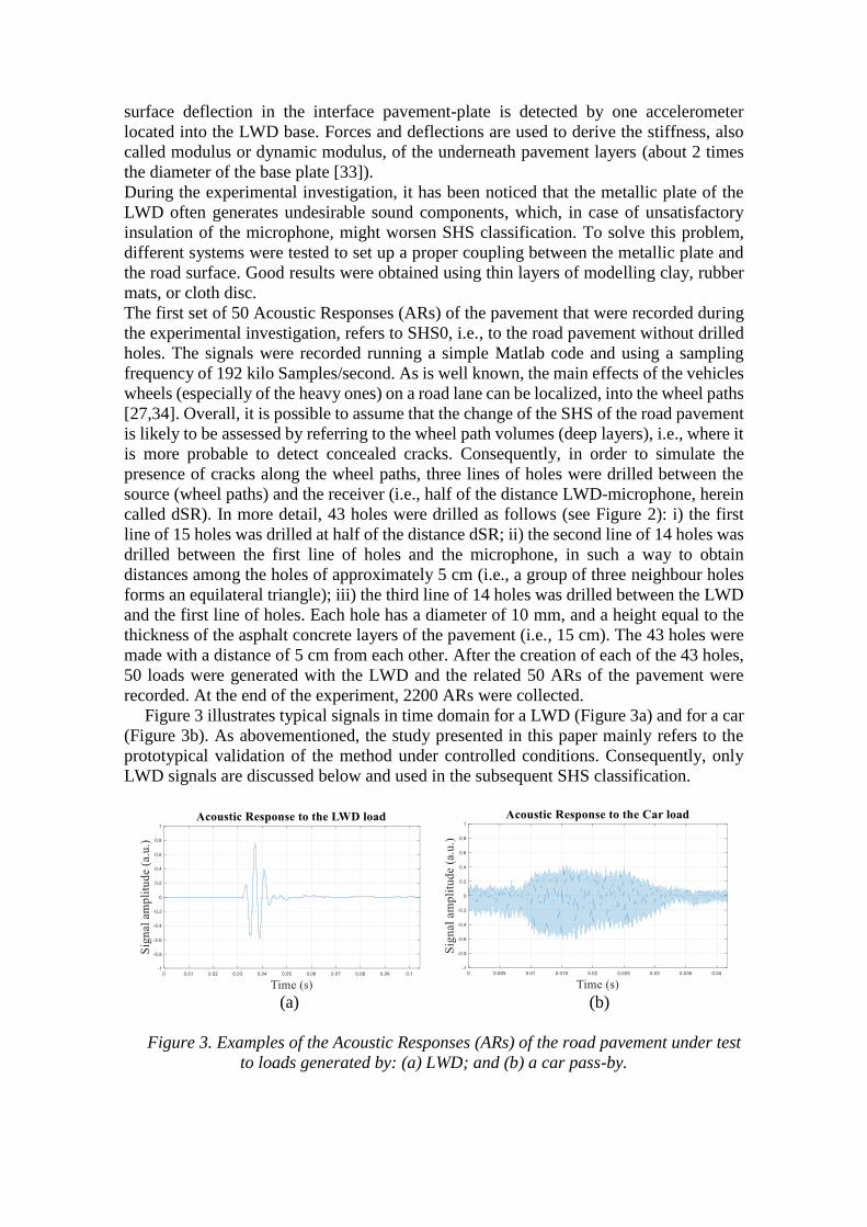
Figure 3 illustrates typical signals in time domain for a LWD (Figure 3a) and for a car

(Figure 3b). As abovementioned, the study presented in this paper mainly refers to the

prototypical validation of the method under controlled conditions. Consequently, only

LWD signals are discussed below and used in the subsequent SHS classification.

(a) (b)

Figure 3. Examples of the Acoustic Responses (ARs) of the road pavement under test

to loads generated by: (a) LWD; and (b) a car pass-by.

Preliminary analyses showed that the acoustic signals were too complex and large to

use without preliminary processing. In order to carry out a comprehensive analysis, the

features were extracted from the time, the frequency, and time-frequency domain. Several

features were taken into account considering the shape and the main characteristics of the

Acoustic Responses (ARs) of the pavement under test (time domain), and their processing

(i.e. periodogram and scalogram in frequency and time-frequency domains, respectively).

Among all the possible features, we selected the best three ones for each domain, which

are listed in Table 1.

Table 1. Features that were taken into account in this study to represent the acoustic

responses of the road pavement under test to the LWD load.

Symbol Feature Unit of

measure

Domain /

Feature Source

1. Δa Amplitude difference between the absolute

maximum P and the absolute minimum N of the

AR amplitudes.

a.u.

Time / Signal

2. Δt Time Delay of N from P Ms

3. σ Standard deviation of the ARs. a.u.

4. PSDmin Minimum of the PSD of the ARs into the

frequency range 50-150 Hz.

dBW/Hz

Frequency /

Periodogram

5. S Slope of the linear regression model of the PSD

of the ARs into the frequency range 20-250 Hz.

Hz

6. fc Spectral Centroid of the Periodogram (PSD vs.

frequency) in the frequency range 20-450 Hz.

Hz

7. EntCWCs Maximum Entropy of the CWCs. a.u.

Time-Frequency /

CWT Scalogram

8. p-fWR Pseudo-frequency of the WR (from the y-axis of

the scalogram).

Hz

9. EngCWCs,max Energy of the CWCs above a given threshold

(60 out of 64, i.e. red areas of the Scalogram).

a.u.

Symbols. AR = Acoustic Response; a.u. = arbitrary unit; dim. = dimensionless;

ms = milliseconds; dB = decibel; dBW/Hz = decibel Watt per Hertz; Hz = Hertz; s = seconds;

Ent = Entropy; CWCs = Continuous Wavelet Coefficients; p-f = pseudo-frequency;

WR = Wavelet Ridges; Eng = Energy; max =maximum; min = minimum.

Figure 4 refers to two out of the three features extracted in time domain.

Figure 4. Graphical representation of two features extracted in the time domain.

P (absolute maximum of the signal amplitude)

N (absolute minimum of the signal amplitude)

Δt

Δa

One Acoustic Response (AR) in the time domain

In order to derive the three features in the frequency domain, the periodogram (Power

Spectral Density versus Frequency; see Figure 5) of each AR was obtained using the

following equation [35]:

FsN

FFTPSD

2

2 , (1)

where FFT is the Fast Fourier Transform of the selected response; N is the length of the

selected response (samples); Fs is the sample frequency used to record the signals (Hz).

PSD is the power of the AR per unit of frequency, i.e., Watt per Hertz or dBW/Hz if the

decibel scale is used to represent the PSD. In this study, in the pursuit of better analysing

the PSD of the ARs of the pavement under investigation, the logarithmic scale for the y-

axis (dBW/Hz) was used and values between -100 and 0 (y-axis) and in the range 25-450

(x-axis) were considered (Fig. 4). Furthermore, the periodogram in Fig. 4 shows: i) the

section of the periodogram where the local minima of PSD were calculated (i.e., the

feature herein called PSDmin); ii) an example of linear regression line of the PSD into

the frequency range 20-250 Hz and its slope (i.e., the feature herein called S, cf. Table 1);

iii) the spectral centroids of the periodogram (i.e., the feature herein called fc, which is

represented by a triangle). From the periodogram, the spectral centroid (“centre of mass”

of the periodogram, cf. [36]) was derived using the following expression:

,1

0

1

0

N

nn

N

nnn

c

p

fp

f (2)

where fc is the spectral centroid (Hz); N is the number of signal samples included in the

frequency range in which the spectral centroid is calculated (samples); pn represents the

weights (e.g. decibel Watt per Hz or dBW/Hz), i.e., the values on the y-axis of the

periodogram; fn refers to the frequencies (Hz; x-axis of the periodogram).

Figure 5. Graphical representation of the features used in the frequency domain.

Wavelet transforms resulted to be the most suitable method to see signal changes

because of the well-known property called “time-frequency localization” [17,37]. This is

the main strength of the WT, which makes the WT: i) more similar to the human ear than

S (slope of the linear regression model)

PSDminfc

Periodogram (PSD vs. Frequency) of one AR

other “too much artificial” tools; ii) particularly suitable for the recognition and the

monitoring of non-stationary phenomena or of signals with short-lived transient

components (which are the combination of transient high frequency components - visible

at the top of the scalogram - and long lasting low frequency components - shown at the

bottom of the scalogram as a continuous magnitude; [37]). For these reasons, the WT

were used in this study. In particular, the Continuous Wavelet Transform (CWT) was

preferred to the Discrete Wavelet Transform (DWT) because of the fact it allows more

detailed analysis than the DWT. The results of the application of the CWT (Equation 3)

is a matrix that contain the Continuous Wavelet Coefficients (CWCs), which are the result

of the convolution between the signal to be analysed and a variable-sized window

functions called Wavelet (or mother wavelet; cf. [37]). A typical 2-D graphical

representation of the CWCs in the time-frequency domain is the “scalogram” (see Figure

6). It shows the scaled percentage of energy of the wavelet coefficients (different colours

or intensity variation of a colour) with respect to time, or shift (x-axis), and scale variables

(y-axis) [17].

dta

btψtx

abaCWT

1

, , (3)

where a is the scaling parameter (a vector with positive elements, which allows

contracting the mother wavelet ψ [38]); b is the shifting parameter, which permits the

translation of the mother wavelet ψ along the x-axis (time); x(t) is the signal to be

transformed; t stands for time (seconds); ψ* is the complex conjugate of ψ. Usually,

scalograms show on the y-axis the scaling parameter, a. However, in this work, a pseudo-

frequency was derived from the scaling parameter using the following expression [39]:

,Sc

a Fa

FF (4)

where Fa is the pseudo-frequency (Hz) corresponding to the scale factor a

(dimensionless); Fc is the central frequency of the mother wavelet ψ used (Hz); FS is the

sampling frequency (Hz). In this study, the mother wavelet “meyr” was used in the CWT.

Figure 6. Graphical representation of two features used in the time-frequency domain.

Time (ms)

Pse

ud

o-f

req

uen

cy (

Hz)

Scalogram of one AR

p-fWR

Wavelet ridge

EngCWCs

The features extracted in the time-frequency domain were derived from the scalograms

and from the CWCs as follows. The Shannon’s Entropy of the CWCs (herein called

EntCWC) per each scale factor a was calculated using the following expression [40]:

i

N

iiCWC ppaEnt

12log , with

aEng

iaCWCpi

2,

, (5)

where N is the length of each AR, and pi is the energy probability distribution of the

CWCs, for i = 1, 2, …, N. The term EngCWC(a) represents the Energy of the CWCs per

each scale factor a. In more detail [40], the variable EngCWC(a) can be calculated from the

CWCs, for b = 1, 2, …, N (with N equal to the length of each AR), using the following

expression:

b

CWC baCWCaEng .,2

(6)

Finally, the validation of the method proposed in this study is based on the

experimental investigation described above and on the following procedure that aims at

carrying out the hierarchical clustering of the acoustic responses (ARs) of the road

pavement and the relative features presented above. In particular, this procedure consists

in: i) computing the distance matrix, which contains the Euclidean distances between

pairs of observations (i.e., samples of each AR or values of each features) [41]; ii)

encoding a tree of hierarchical clusters (i.e., a matrix with cluster indices and linkage

distances between pairs of clusters) using as input the distance matrix calculated in the

first step, counting the highest distance between two element of the distance matrix, and

considering 4 clusters, i.e., one for the structural health condition un-cracked, and the

other three for the structural health status (SHS) cracked with one, two, and three lines of

holes drilled into the road pavement under investigation; iii) finding the smallest height

at which a horizontal cut through the agglomerative hierarchical cluster tree (generated

in the previous step) groups the observations into 4 clusters; iv) generating the confusion

matrix (i.e., a matrix that shows how many observations were associated to each cluster)

and verifying if the ARs associated to a given SHS is correctly clustered and associated

to a single cluster.

4. RESULTS AND DISCUSSIONS

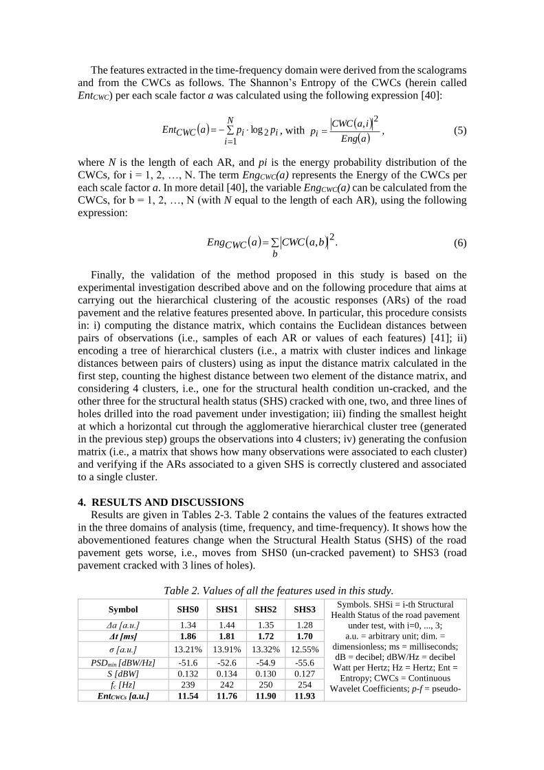
Results are given in Tables 2-3. Table 2 contains the values of the features extracted

in the three domains of analysis (time, frequency, and time-frequency). It shows how the

abovementioned features change when the Structural Health Status (SHS) of the road

pavement gets worse, i.e., moves from SHS0 (un-cracked pavement) to SHS3 (road

pavement cracked with 3 lines of holes).

Table 2. Values of all the features used in this study.

Symbol SHS0 SHS1 SHS2 SHS3 Symbols. SHSi = i-th Structural

Health Status of the road pavement

under test, with i=0, ..., 3;

a.u. = arbitrary unit; dim. =

dimensionless; ms = milliseconds;

dB = decibel; dBW/Hz = decibel

Watt per Hertz; Hz = Hertz; Ent =

Entropy; CWCs = Continuous

Wavelet Coefficients; p-f = pseudo-

Δa [a.u.] 1.34 1.44 1.35 1.28

Δt [ms] 1.86 1.81 1.72 1.70

σ [a.u.] 13.21% 13.91% 13.32% 12.55%

PSDmin [dBW/Hz] -51.6 -52.6 -54.9 -55.6

S [dBW] 0.132 0.134 0.130 0.127

fc [Hz] 239 242 250 254

EntCWCs [a.u.] 11.54 11.76 11.90 11.93

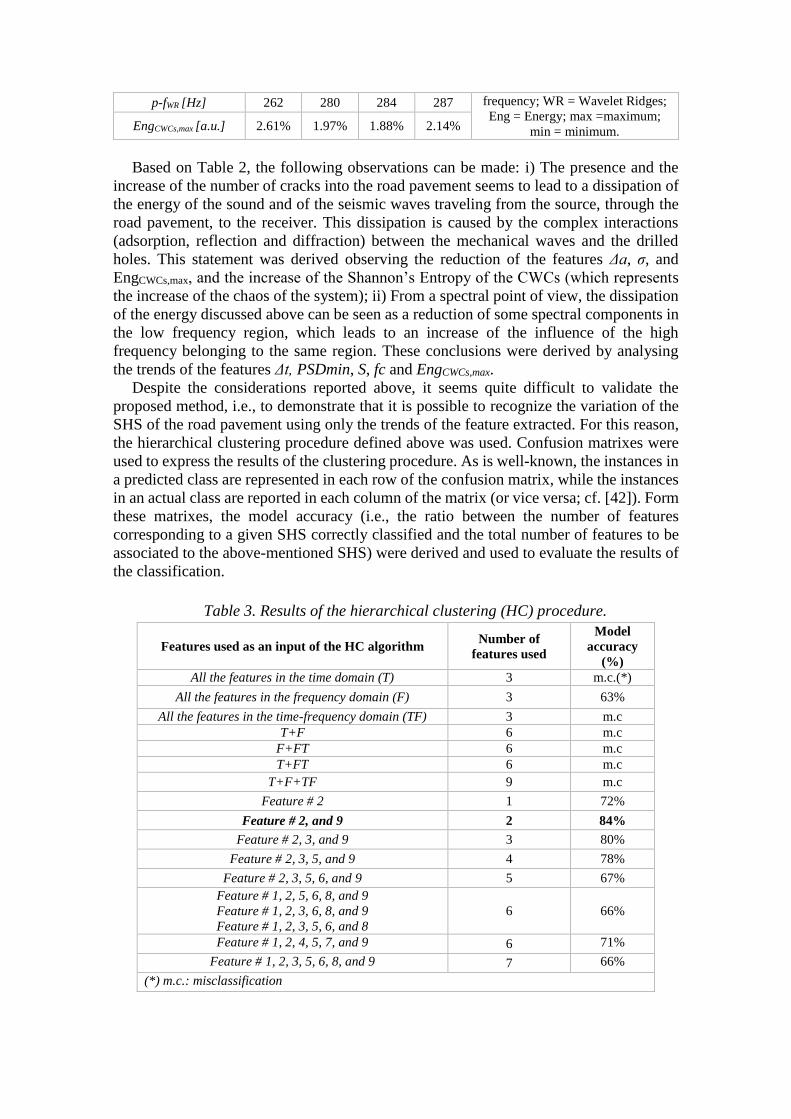
p-fWR [Hz] 262 280 284 287 frequency; WR = Wavelet Ridges;

Eng = Energy; max =maximum;

min = minimum. EngCWCs,max [a.u.] 2.61% 1.97% 1.88% 2.14%

Based on Table 2, the following observations can be made: i) The presence and the

increase of the number of cracks into the road pavement seems to lead to a dissipation of

the energy of the sound and of the seismic waves traveling from the source, through the

road pavement, to the receiver. This dissipation is caused by the complex interactions

(adsorption, reflection and diffraction) between the mechanical waves and the drilled

holes. This statement was derived observing the reduction of the features Δa, σ, and

EngCWCs,max, and the increase of the Shannon’s Entropy of the CWCs (which represents

the increase of the chaos of the system); ii) From a spectral point of view, the dissipation

of the energy discussed above can be seen as a reduction of some spectral components in

the low frequency region, which leads to an increase of the influence of the high

frequency belonging to the same region. These conclusions were derived by analysing

the trends of the features Δt, PSDmin, S, fc and EngCWCs,max.

Despite the considerations reported above, it seems quite difficult to validate the

proposed method, i.e., to demonstrate that it is possible to recognize the variation of the

SHS of the road pavement using only the trends of the feature extracted. For this reason,

the hierarchical clustering procedure defined above was used. Confusion matrixes were

used to express the results of the clustering procedure. As is well-known, the instances in

a predicted class are represented in each row of the confusion matrix, while the instances

in an actual class are reported in each column of the matrix (or vice versa; cf. [42]). Form

these matrixes, the model accuracy (i.e., the ratio between the number of features

corresponding to a given SHS correctly classified and the total number of features to be

associated to the above-mentioned SHS) were derived and used to evaluate the results of

the classification.

Table 3. Results of the hierarchical clustering (HC) procedure.

Features used as an input of the HC algorithm Number of

features used

Model

accuracy

(%)

All the features in the time domain (T) 3 m.c.(*)

All the features in the frequency domain (F) 3 63%

All the features in the time-frequency domain (TF) 3 m.c

T+F 6 m.c

F+FT 6 m.c

T+FT 6 m.c

T+F+TF 9 m.c

Feature # 2 1 72%

Feature # 2, and 9 2 84%

Feature # 2, 3, and 9 3 80%

Feature # 2, 3, 5, and 9 4 78%

Feature # 2, 3, 5, 6, and 9 5 67%

Feature # 1, 2, 5, 6, 8, and 9

Feature # 1, 2, 3, 6, 8, and 9

Feature # 1, 2, 3, 5, 6, and 8

6 66%

Feature # 1, 2, 4, 5, 7, and 9 6 71%

Feature # 1, 2, 3, 5, 6, 8, and 9 7 66%

(*) m.c.: misclassification

Based on Table 3, it is possible to state the relationship between AR (through the

indicators shown in Table 1) and SHS (unknown). For example, when features 2 and 9 in

Table 1 (i.e., time lag and energy) were used, 84 cases out of 100 cases were correctly

classified (best set of features: Δt & EngCWCs,max).

5. CONCLUSIONS

A non-destructive, acoustic, feature-based SHM method was presented in this paper.

The validation of the proposed method was carried out through a specifically designed

experimental investigation. In particular, the proposed method was applied to an asphalt

concrete pavement and a change of its structural health status over time was simulated

(generation and propagation of cracks): i) three lines of drilled holes were created into the

pavement under test to simulate the cracks that usually are generated by vehicular traffic

along the wheel paths; ii) a Light Weight Deflectometer (LWD) was used as “pilot-

source” to load the pavement; iii) the acoustic responses (acoustic signals) of the

pavement to the load were detected by an insulated microphone; iv) the signals were

analysed through different graphical representations obtained using different

mathematical tools in three domains (i.e., time, frequency, and time-frequency domains);

v) different features were extracted and analysed, using a hierarchical clustering

procedure and confusion matrixes, in order to understand which feature is the most

meaningful in recognizing the presence and the growth over time of cracks in the

monitored structure. Results show that it is possible to identify and quantify cracks into

asphalt concrete road pavement using the proposed acoustic response and feature-based

SHM method. Future research will focus on the improvement of the proposed method in

terms of measurement system, signal analysis, in the pursuit of classifying different types

of road pavements and structures based on their acoustic response.

6. REFERENCES

1. F.A. Marcianò, G. Musolino, A. Vitetta, "Signal setting optimization on urban road

transport networks: The case of emergency evacuation", Saf. Sci., (2015)

doi:10.1016/j.ssci.2014.08.005

2. F.G. Praticò, "On the dependence of acoustic performance on pavement

characteristics", Transp. Res. Part D Transp. Environ., (2014)

doi:10.1016/j.trd.2014.04.004

3. F.G. Praticò, A. Moro, R. Ammendola, "Modeling HMA Bulk Specific Gravities: a

Theoretical and Experimental Investigation", Int. J. Pavement Res. Technol., (2) 115–

122 (2009)

4. F.G. Praticò, A. Moro, R. Ammendola, "Factors affecting variance and bias of non-

nuclear density gauges for PEM and DGFC", Balt. J. Road Bridg. Eng., (4) 99–107

(2009)

5. F.G. Praticò, A. Moro, R. Ammendola, "Potential of fire extinguisher powder as a filler

in bituminous mixes", J. Hazard. Mater., (2010) doi:10.1016/j.jhazmat.2009.08.136

6. J. Ba, C. Su, Y. Li, S. Tu, "Characteristics of heat flow and geothermal fields in

Ruidian, Western Yunnan Province, China", Int. J. Heat Technol., (2019)

doi:10.18280/ijht.360407

7. J. Guerrero-Ibáñez, S. Zeadally, J. Contreras-Castillo, "Sensor technologies for

intelligent transportation systems", Sensors (Switzerland), (2018)

doi:10.3390/s18041212

8. S. Cafiso, C. D’Agostino, E. Delfino, A. Montella, "From manual to automatic

pavement distress detection and classification", in 5th IEEE Int. Conf. Model. Technol.

Intell. Transp. Syst. MT-ITS 2017 - Proc., (2017) doi:10.1109/MTITS.2017.8005711

9. Y. Zhang, C. Chen, Q. Wu, Q. Lu, S. Zhang, G. Zhang, Y. Yang, "A kinect-based

approach for 3D Pavement surface reconstruction and cracking recognition", IEEE

Trans. Intell. Transp. Syst., (in press) (2018)

10. K. Chen, M. Lu, X. Fan, M. Wei, J. Wu, "Road condition monitoring using on-board

three-axis accelerometer and GPS sensor", in Proc. 2011 6th Int. ICST Conf. Commun.

Netw. China, CHINACOM 2011, (2011) doi:10.1109/ChinaCom.2011.6158308

11. T. Bills, R. Bryant, A.W. Bryant, "Towards a frugal framework for monitoring road

quality", in 2014 17th IEEE Int. Conf. Intell. Transp. Syst. ITSC 2014, (2014)

doi:10.1109/ITSC.2014.6958175

12. C.W. Yi, Y.T. Chuang, C.S. Nian, "Toward Crowdsourcing-Based Road Pavement

Monitoring by Mobile Sensing Technologies", IEEE Trans. Intell. Transp. Syst., (2015)

doi:10.1109/TITS.2014.2378511

13. M.R. Carlos, M.E. Aragon, L.C. Gonzalez, H.J. Escalante, F. Martinez, "Evaluation

of Detection Approaches for Road Anomalies Based on Accelerometer Readings--

Addressing Who’s Who", IEEE Trans. Intell. Transp. Syst., (2018)

doi:10.1109/TITS.2017.2773084

14. C. Lenglet, J. Blanc, S. Dubroca, "Smart road that warns its network manager when

it begins cracking", Inst. Eng. Technol. Intell. Transp. Syst., (11) 152–157 (2017)

doi:10.1049/iet-its.2016.0044

15. R. Fedele, M. Merenda, F.G. Praticò, R. Carotenuto, F.G. Della Corte, "Energy

harvesting for IoT road monitoring systems", Instrum. Mes. Metrol., (17) 605–623 (2018)

doi:10.3166/I2M.17.605-623

16. W. Uddin, "An Overview of GPR Applications for Evaluation of Pavement Thickness

and Cracking", in 15th Int. Conf. Gr. Penetrating Radar - GPR 2014, (2014)

17. M.M. Reda Taha, A. Noureldin, J.L. Lucero, T.J. Baca, "Wavelet transform for

structural health monitoring: A compendium of uses and features", Struct. Heal. Monit.,

(2006) doi:10.1177/1475921706067741

18. N. Hassan, S. Mathavan, K. Kamal., "Road crack detection using the particle filter",

in IEEE ICAC 2017, (2017)

19. M. Salman, S. Mathavan, K. Kamal, M. Rahman, "Pavement crack detection using

the Gabor filter", in IEEE Conf. Intell. Transp. Syst. Proceedings, ITSC, (2013)

doi:10.1109/ITSC.2013.6728529

20. T.A. Carr, M.D. Jenkins, M.I. Iglesias, T. Buggy, G. Morison., "Road crack detection

using a single stage detector based deep neural network", in IEEE EESMS 2018, (2018)

21. X. Wang, Z. Hu, "Grid-based pavement crack analysis using deep learning", in 2017

4th Int. Conf. Transp. Inf. Safety, ICTIS 2017 - Proc., (2017)

doi:10.1109/ICTIS.2017.8047878

22. P. Subirats, J. Dumoulin, V. Legeay, D. Barba, "Automation of pavement surface

crack detection using the continuous wavelet transform", in Proc. - Int. Conf. Image

Process. ICIP, (2006) doi:10.1109/ICIP.2006.313007

23. Y.O. Ouma, M. Hahn, "Wavelet-morphology based detection of incipient linear

cracks in asphalt pavements from RGB camera imagery and classification using circular

Radon transform", Adv. Eng. Informatics, (2016) doi:10.1016/j.aei.2016.06.003

24. S.W. Katicha, G. Flintsch, J. Bryce, B. Ferne, "Wavelet denoising of TSD deflection

slope measurements for improved pavement structural evaluation", Comput. Civ.

Infrastruct. Eng., (2014) doi:10.1111/mice.12052

25. J. Gajewski, T. Sadowski, "Sensitivity analysis of crack propagation in pavement

bituminous layered structures using a hybrid system integrating Artificial Neural

Networks and Finite Element Method", Comput. Mater. Sci., (2014)

doi:10.1016/j.commatsci.2013.09.025

26. H. Hasni, A.H. Alavi, K. Chatti, N. Lajnef, "A self-powered surface sensing approach

for detection of bottom-up cracking in asphalt concrete pavements:

Theoretical/numerical modeling", Constr. Build. Mater., (2017)

doi:10.1016/j.conbuildmat.2017.03.197

27. Y.H. Huang, "Pavement Analysis and Design", (2003)

28. R. Fedele, F.G. Praticò, R. Carotenuto, F.G. Della Corte, "Damage detection into road

pavements through acoustic signature analysis: First results", in 24th Int. Congr. Sound

Vib. ICSV 2017, (2017)

29. R. Fedele, F.G. Pratico, R. Carotenuto, F.G. Della Corte, "Instrumented

infrastructures for damage detection and management", in 5th IEEE Int. Conf. Model.

Technol. Intell. Transp. Syst. MT-ITS 2017 - Proc., (2017)

doi:10.1109/MTITS.2017.8005729

30. ASTM E2583-07, "Standard Test Method for Measuring Deflections with a Light

Weight Deflectometer (LWD)", ASTM International, West Conshohocken, PA, 2015,

www.astm.org, (2015)

31. C.W. Schwartz, Z. Afsharikia, S. Khosravifar, "Standardizing lightweight

deflectometer modulus measurements for compaction quality assurance", (2017).

https://www.roads.maryland.gov/OPR_Research/MD-17-TPF-5-285-

LWD_REPORT.pdf

32. C. Senseney, M. Mooney, "Characterization of Two-Layer Soil System Using a

Lightweight Deflectometer with Radial Sensors", Transp. Res. Rec. J. Transp. Res. Board,

(2011) doi:10.3141/2186-03

33. A.F. Elhakim, K. Elbaz, M.I. Amer, "The use of light weight deflectometer for in situ

evaluation of sand degree of compaction", HBRC J., (2014)

doi:10.1016/j.hbrcj.2013.12.003

34. F. Finn, C.L. Saraf, R. Kulkarni, K. Nair, W. Smith, A. Abdullah, "Development of

pavement structural subsystems", (1986)

35. A.G. Bendat, J.S. Piersol, "Random Data Analysis and Measurement Procedures",

Meas. Sci. Technol., (2000) doi:10.1088/0957-0233/11/12/702

36. E. Schubert, J. Wolfe, "Timbral brightness and spectral centroid", Acta Acust. United

with Acust., (92) 820–825 (2006)

37. P. Kumar, E. Foufoula-Georgiou, "Wavelet analysis for geophysical applications",

Rev. Geophys., (1997) doi:10.1029/97RG00427

38. H. Kim, H. Melhem, "Damage detection of structures by wavelet analysis", Eng.

Struct., (2004) doi:10.1016/j.engstruct.2003.10.008

39. A. Alhasan, D.J. White, K. De Brabanterb, "Continuous wavelet analysis of pavement

profiles", Autom. Constr., (2016) doi:10.1016/j.autcon.2015.12.013

40. M. Abdolmaleki, M. Tabaei, N. Fathianpour, B.G.H. Gorte, "Selecting optimum base

wavelet for extracting spectral alteration features associated with porphyry copper

mineralization using hyperspectral images", Int. J. Appl. Earth Obs. Geoinf., (2017)

doi:10.1016/j.jag.2017.02.005

41. Mathworks, "Hierarchical Clustering", (2006).

https://it.mathworks.com/help/stats/hierarchical-clustering.html

42. D.M. Powers, "Evaluation: from precision, recall and F-measure to ROC,

informedness, markedness and correlation", J. Mach. Learn. Technol., (2011)