Monitoring and modeling air quality in Mendoza, Argentinalidecc.cs.uns.edu.ar/~nbb/ccm/downloads/Clases/Literatura/EP... · desert climate and to improve urban ... the region is characterized

Chapter in Regional and local aspects of air quality, Editorial WIT Press, Southampton, Boston, Computational Mechanics Publications, (in press 2002).

E. Puliafito and C. Puliafito 1

Monitoring and modeling air quality in Mendoza, Argentina

E. Puliafito and C. Puliafito Institute for Environmental Studies (IEMA)

University of Mendoza, Argentina Abstract Like many big urban centers, Mendoza, a city of about 900,000 inhabitants, has been increasing its air pollution mostly from mobile sources. To asses on its air quality, two main strategies has been developed: the setup of a network of monitoring stations and the development of a comprehensive model. Continuous monitoring and daily measurements of main pollutants had been performed since more than 10 years, at different sites, combined with several measuring campaigns. On the other side, a model, based on a geographical information system has been developed to evaluate the air quality derived from stationary and mobile sources. Once the model has been calibrated with the given measurements, the system is then used to test the compliance to local standard air quality, or to study the environmental impact of new industries or to determine the changing conditions when vehicle circulation is increased. This allows to characterize areas with potential increase in air pollution or improvement in air quality. It is also possible to compute past or present conditions by changing basic information as traffic flow, or stack emission rates. In this article a review of the monitoring and modeling efforts, together with a prognosis of future possible scenarios will be presented. Also a case study during a high pollution event occurred in May 1995 is here described.

1 Introduction The city of Mendoza is located in western Argentina in an arid to semi-arid zone of low rainfall, as it will be described below. Its people has a clear oasis culture, where great care is given in managing its limited resources, especially water and space, and developing an appropriate habitat based on a steady effort. Therefore environmental preservation and sustainable development is a consequence of its long cultural survival process. The General Water Law from 1884, still in force, and the Irrigation Department created in 1916, which is responsible for managing the irrigation water resources, is a clear example of this environmental culture. We should also mention, as important milestones of the end of the nineteen’s and beginning of the twenty’s century, the development of sanitary works, the creation of a 450 ha park and public tree fostering in the urban area. Its many trees and green spaces could be identified as a natural way to moderate desert climate and to improve urban life quality. A century later, this visionary urban planning showed to be insufficient to stop the progressive degradation of the natural environment, and to solve the upraise of new conflicts. The increasing urbanization problems, with traffic congestion, air pollution, and loss of green or agricultural space, placed additional pressure to the administration of natural resources and existing infrastructures. This situation finally pushed the society to a broad discussion. As a consequence new environmental laws were passed by the Provincial Congress and in 1989 an Environmental Ministry was incorporated to the Provincial Executive Power. Lots of efforts was done to rearrange the institutional relations within the same Provincial State, the Municipalities and the Federal State, regulating the application of Provincial and Federal Laws or nationals decrees. The main objective of this Ministry was the action and coordination with Municipalities, Enterprises and Scientific institutions, in the following fields: a) environmental Information; b) development and up-dating of legal, institutional and techno-economics instruments for environmental protection; c) development of public environmental awareness; d) natural flora and fauna preservation; e) environment control and sanitation; f) urban regulation and environmental development; Urban services with direct environmental incidence (drinkable water, sewers, parks, and public transportation); and g) housing. The environmental policy was based on prevention (instead of acting on the consequences), participation (protection and improvement do require permanent consultation with the population, in order to know their hopes and expectation), and political and technical cooperation (the solution of environmental problems requires interdisciplinarity and new technology). Only through a vast cooperation among public offices, research institutes and non governmental organizations is possible to solve many of these problems and to prevent for continuous deterioration of urban life quality. Environmental legislation enforcement, has been very active in the area of pollution reduction and



control, especially in the following areas: a) atmospheric pollution by mobile sources; b) pollution by urban solid domestic residues; c) contamination by dangerous and special waste; d) atmospheric pollution due to stationary sources; e) industrial water pollution; f) contamination by oil exploitation; and g) contamination by mining exploitation. However, new regulations mandate the monitoring and tracking of numerous issues, introducing extra demands on agencies at the local government level. Since the early 90, the University of Mendoza through its Institute for Environmental Research (IEMA), in cooperation with the Center for Environmental Research UFZ-Leipzig-Halle, and the Max-Planck Institute for Aeronomy MPAE-Lindau (Germany), among other local universities and research centers, have joined the effort of the public office, implementing a broad environmental research program. Relevant aspects of this program included research in the area of urban pollution monitoring (Schlink [1,2], Puliafito [3], Weißflog [4]; Wenzel [5]) ecosystem modeling, environmental standards and legislation (Puliafito [6]), health effects due to ambient air, (Herbarth [7,8]) and sustainable architecture. In this article we will concentrate only with aspects related to the air pollution situation in the city of Mendoza. We will show the modeling efforts performed by our Institute, aimed to contribute to the local authorities in implementing an effective air pollution control strategy. The air in an urban area is influenced by many factors. They range from local meteorology and orography, natural and anthropogenic emissions, which sends to the atmosphere, among others, pollutants like Carbon monoxide, Oxides of Sulfur and nitrogen, photochemical oxidants and Hydrocarbons, and dust. The major source of man-made pollution comes typically from industry, commerce, domestic cooking and heating, and transportation activities. Urban environment is stressed by a number of common problems such us population, industrial and commercial growth, increasing energy and transportation demands. Worldwide, before 1990 most of the concern and control efforts was given to the industrial sources, but lately it was very clear that the major source for the degradation of the air quality was not any more factories, but the road vehicles, - buses, passengers cars, light and heavy duty trucks or motorcycles. Additionally concern has been given in the last decade to understand and evaluate the impact of such emissions on the population health. A program to control the air pollution is generally based on several goals: a) Setting air quality targets, based normally on health effects; b) data monitoring of principal pollutants and meteorology; c) completion of source inventories, through measurements and surveys; d) setting an appropriate model, to control the air quality targets and to correlate air quality standards with emission reduction targets; and e) implementation of legal and socio-economic measures to achieve the desired air quality targets. The selected model should help to evaluate and compare transport policies and plans, to determine air quality standards, to asses on environmental impact or health risk. The air quality modeling segments should include at least: a) emission forecasting models to predict the monitoring measurements; b) study and forecast of wind patterns and transport models; c) dispersion models to correlate emission with ground ambient concentrations in order to understand the contribution of each sources. With the exception of ozone, which is a secondary pollutant, the present models represent approximately the pollutant situation, therefore it is possible to model NOx, CO and hydrocarbons based on the emission rate at the source. Different approaches may be adopted to handle these big amount of information, depending on the available technology, skills and environmental programs. Moreover, this information needs to be handled not only in temporal data formats for some monitoring stations, but over a wide spatial distribution. The actual efforts in improving the air quality in Mendoza, and why a model based on a Geographical Information System (GIS) can meet the required needs, will be in this article presented. GIS is a computer based system that helps to translate environmental science into policy by using relevant geographically located information, combined with algorithms, procedures and models that represent general scientific understanding. Data sets created and organized under GIS can be shared between various government entities and the public. GIS applications allows any user, department or agency to access common geographical data and made it easy for the public to browse the data, providing an excellent software for development and analysis. Today, GIS is surely one of the most used software platform for planning all over the world. These features justify choosing GIS as an appropriate management tool for air pollution control.

2 Materials and Methods

2.1 Meteorology and orography The city of Mendoza, (33°S, 68°W, 750 m. a. N. s. l.), is located at the east side of the Andes Mountains in western Argentina. The Cordillera close to Mendoza, reaches an average height of 5,000 m with peaks up to



7,000 m. This natural barrier influences the meteorological conditions determining a strong dependence in the air pollution situation. As it was said, the region is characterized by its low precipitations: 120 to 400 mm/a, (mean 230 mm/a), which occurs specially during the summer months (November to March). Only 3% of the total province territory (250,000 km2) is irrigated by five main rivers with annual modules less than 50 m3, conforming three main oasis. Almost 70% of the population is concentrated in the northern oasis, conforming the Mendoza metropolitan area with approximate 900,000 inhabitants. This region is characterized by passing cyclones developing from cold polar air masses at the polar front of the southern hemisphere. Consequently the weather is disturbed by passing fronts, especially during the winter. However, during the summer season the polar front is pushed to the south, developing a stable area of high pressures in the north-east of Argentina. Unlike the northern hemisphere, the southern hemisphere is covered by more sea than land. The circulation is dominated by the planetary system. Therefore, the NE winds arise from the semi-permanent anticyclone on the atlantic east of the South American continent at approximately 30º S and thus belong to an “Atlantic wind system”. This subtropical circulation brings warm and moist air into the region. Since the polar front is shifted to the north in the winter, the metereological conditions of Mendoza, during this time, are determined by Pacific air masses (cyclones). Consequently in this season there is little rainfall. Due to its closeness to the mountains, Zonda winds similar to Föhn or Chinook winds, prevail in the higher layers mostly during the winter months (May to October) with high probability of frost, which contributes to a higher degree of pollution due to the occurrence of strong thermal inversion layers. Damp, warm tropical air masses pass over The Andes cordillera from west to east, and therefore, the air masses ascend saturated adiabatically, losing their moisture in the western hillside of The Andes. This wind descends dry adiabatically on the eastern hillside provoking strong increases of the temperature of about 4ºC per each kilometer of mountain height, and with speeds ranging 5-6 m/s, and gust up to 12 m/s. The mean wind intensity is around 2 m/s, with mostly calm days (< 0.5 m/s) 35%, and predominant wind from S 13%, NE and W 12%, SW 10%, SE 8 %. Low relative humidity (50%), low incidences of fog and few days with covered skies (65-75 days/annum). The solar global radiation varies from 270 MJ/m2 in winter to 780 MJ/m2 in summer, with annual mean daily heliophany of 7.9 hours. The climate can be classified according to the Köeppen scale as BWakw: dry dessert, with mean temperature of the hottest month > 22°C, cold and dry winter with mean temperature below 18°C. The area presents low relative humidity (50%), low incidences of fog and few days with covered skies (65-75 days/annum). Another important feature for the description of the air pollution is the day-night variation, characterized by a typical valley-mountain circulation. From the first hours after sunset to early hours after sunrise, there is a clear wind flow from WSW, while in daylight hours the circulation is ENE. Strong solar heating on the valley side causes an up-slope wind flow at daytime (ENE). At night due to rapid radiational cooling on the valley slope, the circulation switches over causing the air masses to move down the mountain from WSW. This strong night cooling and day heating produces an important variation in mixing heights and inversion layers. More on meteorological and climatic aspects relevant to the region can be seen in Schlink [1,2].

2.2. Monitoring and sampling Ambient concentration measurements of main pollutants have been monitored since 1970 in the metropolitan area of Mendoza by the Ministry of Environment and Public Works through its Direction for Environmental Control. In the urban area of Mendoza, around 15 stations monitors daily mean values of Total Suspended Particles (TSP) - by filter capture and reflectometry-, daily mean values of nitrogen oxides NOx -by colorimetric Griess-Saltzmann, and once a week 24 h mean values of lead Pb -by colorimetric ditozone-, and sulfur dioxide SO2 -by colorimetric West and Gacke modified by Pate-. Also, our Institute IEMA, measures since 1995, black carbon and PAH poliaromatic compounds (Aethalometer GIV reflectometry), surface ozone (O3), nitrogen oxides (NOx), Carbon monoxide (CO), using a set of Horiba instruments (series APO350E for O3 and APN360 for NOx and CO) and meteorological parameters, including solar global radiation. Besides the mentioned monitoring data, paper filter samples of particulate matter have been collected using a high volume pump at several measuring points. At the beginning of the project, few organized information was available over the emission of the fixed sources, thus it was necessary to set up an emission inventory of the main sources. These forms contain relevant information on the type of fuel, yearly consumption, physical data of boilers, chimneys and emission measurements if available. Additionally various stack measurements were performed by independent consultants using an isokinetic stack samplers, following U.S. EPA Standard Methods. The main industrial areas are located on the periphery of the city: oil refineries, petrochemical industries and energy production are situated SW of the city, two cement industries are on the north edge and finally the agro-



industrial production is mainly on the east side of Mendoza. Figure 1 shows a satellite picture of the city and surroundings, showing also the main industrial sources and the monitoring stations.

Figure 1: Satellite image of the area under study. Monitoring and meteorological stations are shown with

triangles, main industrial sources are represented with circles.

2.3 Cycles of the airborne pollutants The described meteorological and orographic conditions of the city, together with man’s activity produce a characteristic air pollution pattern. A detailed analysis of the gathered ambient data shows several well define cycles. A main cycle is the seasonal variation (winter-summer), with higher values in winter and lower values in summer. Figure 2 shows monthly mean values of daily measurements of total suspended particles, monitored at the downtown area. This cycle is directly coupled to the meteorological conditions above described, namely calm winds, few precipitations and high occurrences of low inversion layers in winter. Seldom polar fronts from SE bring snowfalls to mountain and valley, breaking the accumulation cycle of air pollution. Another clear cycle is the day-night variation, characterized by a typical valley-mountain circulation as mentioned above..

Figure 2: Monthly average of 24h values of total suspended particles at a

downtown monitoring station.



Figure 3 shows a typical day, with solar radiation, wind direction, surface ozone (O3), carbon monoxide (CO), and nitrogen oxides (NOx) measurements, monitored at the IEMA Institute. This graphic shows a strong traffic related emission, where it can be clearly seen the beginning of normal day activities from 7 to 9 am and back-to-home rush hour after 8 pm. It may also be noted that despite in Mendoza there is an important flux of back to home traffic at noontime, mainly for lunch and because of end of school activities, the vehicle pollution is not heavily shown in the ambient concentrations values. This is an indication of the high convective dispersion present during midday Note that Mendoza has a very dry (low humidity) climate, and then there is less heat exchange due to water vapor. Analyzing the monitoring data, it is possible to distinguish a typical weekly cycle, which confirms the relevance of mobile sources emissions in the air quality of Mendoza. Figure 4 shows the annual daily mean values for TSP and NOx according to the day of week, from a data series of several years taken at one of the fixed monitoring station. So, it can bee seen that from Monday through Thursday the values are very similar, Friday is lower, and a strong decrease is present on weekend days.

Figure 3: Typical daily variation of global solar radiation, and main pollutants monitored at the IEMA Institute,

sited in Benegas, Mendoza. NOx: gray line (ppb); solar radiation: dark line (W/m2); ozone: thin line with triangles (ppb); CO: dashed line with squares (x100 ppm).

The ozone data also show a very interesting pattern, according to our monitoring data. Ozone is a mayor secondary air pollutant in many urban and rural areas of the world. High concentrations of surface ozone have become a significant problem affecting human health, vegetation, and numerous man-made and natural materials. Ozone in the lower atmosphere is produced during hydrocarbon oxidation via the catalytic action of the nitrogen oxides NO and NO2. Although high ozone pollution of the lower troposphere has been widely investigated in the northern hemisphere, ozone has only been recorded in a limited extent in South America. Since 1994, the Institute IEMA, is measuring surface ozone from different locations in the Mendoza urban and suburban areas. The photochemical origination of ozone from pollutants (primarily from vehicles engines) and its strong dependence on the sun’s ultraviolet (UV) irradiation would suggest a high level of ozone production and accumulation in Mendoza. But this is not, in fact, the case. In winter the night-time temperature may drop below 0° C until the air is heated again after sunrise at about 8:00 a.m. In the semi-arid region of Mendoza, the air is very dry (especially in winter), and with temperatures of 15 °C at most, there are very few clouds. Hence, ozone formation takes place parallel to the temperature (radiation profile).



Figure 4: Annual mean values of TSP and NOx in µg/m3 as a function of the day of the week measured at

downtown area in Mendoza. The time period between sunrise and sunset is shorter in winter than in summer. This causes very sharp diurnal ozone peaks. Minor transport by wind causes the midday ozone concentration to reach the highest values of the year. The lower the daily maximum temperature, the lower is the transport and the higher is the midday ozone peak. In the morning and evening rush hours, vehicle emissions are able to enrich and reduce ozone. The ozone concentration immediately drops to zero. If any transport occurs, it mostly takes the form of the mountain-valley circulation systems. It lowers the midday ozone peak and produces ozone peaks during the dark night-time when warm air rich in ozone arrives from hills. During fall, with temperatures above 10 °C ozone and temperature peaks follow the diurnal radiation cycle, as they do in winter. During normal conditions, the temperature continuously increases after sunrise, reaching a maximum at about 2:00 p.m. and then generally declining until the next morning. This pattern is superimposed by the concentration changes due to the mountain-valley transport system, which are much stronger than in the winter (up to 0.11 mg/m3). The weak but continuous circulation starts at approximately 10:00 a.m. and reduces the ozone concentration. This explains the lower ozone maxima in the fall (peaks up to 0.07 mg/m3) and even in the summer (peaks up to 0.055 mg/m3) than in the winter. During the summer, as well as during the fall, the circulation system leads to additional minima in the diurnal ozone profile. The onset of circulation is connected with the transport of clean air and produces a morning minimum of concentration. At sunset, ozone formation is terminated and an evening minimum appears. However, the circulation system reverses and increases the ozone concentration anew by the downhill transport of ozone-rich air from the west. The strong circulation system causes the midday peak to be lower and the night-time peak to be higher in summer than in winter. This explains the findings of highest ozone variations during winter and the generally low medium ozone pollution [2]. One other possible cause that should be considered, in addition to meteorological influences, is the chemical reduction of ozone by particles and other pollutants from vehicle exhausts. This reaction, the probability of which depends on the temperature, leads to a drop in the ozone concentration, especially during summer.

2.4 Geographical Information System GIS is a computer based system for capturing, storing, checking and manipulating data that are spatially referenced. For this study we used the ArcView® application due to its relative user friendliness and its wide use by local authorities and many research institutes. New applications of GIS are been developed to explore dynamic environmental models. Like in every computer language, GIS uses data types, which are stored and manipulated in form of a vector (point, line or polygon) and or raster (cells or grid). So it is possible to associate each of this shapes with consistent information in their databases.



In our study, industries and monitoring sites are examples of point shapes, which correspond to records in the respective database. In each of this record, information regarding time series of monthly, annual mean values of ambient concentration are associated to the monitoring site database. Stack dimensions, emission rates and coordinates are associated to the industry database. In the GIS system, each street is represented by a segment corresponding to a record in the database. We have characterized streets according to three hierarchies: a) primary or main city access and inter county freeway; b) secondary or intra county roads; and c) tertiary or residential streets. The hierarchies had been selected according to traffic intensity, hourly variation, street width, dominant use, such as: private or public transport; light or heavy duty; commercial or residential; and other urban criteria. Streets axis, number and emission of vehicles are included in records of line shape type database. Each of these segments also includes length, street type, county and so on. Several other indicators such as inhabitants per car use, inhabitants growth rate, main city attractors, and a mobility source-destination public survey, have been used to complement the knowledge of the city mobility. A particular display of the different shapes and options are called themes and can be viewed or selected in any order, e.g. localization of monitoring sites, emission patterns, etc. These sites are sorted according to the modeller criteria, and the most relevant features may be highlighted on individual maps (or views) and displayed on different scales. It is important to note, that GIS is not only used as a map viewer, but more as an integrated tool to handle data from many sources.

2.5 Data collection Any air quality model requires good information on emission sources, energy consumption and meteorological data. There are several categories of sources: a) large stationary sources, like steelworks, petrochemical plants, power generation; b) medium-small stationary sources, including industrial boilers and process plants, commercial and residential heating, laundries, dry cleaners; c) domestic activities, such as heating and cooking; and d) road vehicles like gasoline or diesel passengers cars, public buses, light or heavy duty vehicles, two or three wheel vehicles. The emission inventories may be prepared according to the type of sources. For example, for large sources, by sending questionnaires to large energy consumers and checking them with in-situ stack measurements; and for small energy consumers, it can be treated as area sources derived from fuel consumption and calculating it through average emission factors. The estimation of mobile sources can be calculated thorough traffic emissions, using average emission factors for different fuel and power, number of vehicles, average speed and travelled distances, complemented with traffic counting and public registers and surveys.

2.6 Calculation of industrial emissions To treat the stationary sources, the model calls the program ISC3 (EPA: U.S. Environmental Protection Agency) that calculates the ambient concentration for multiple industrial sources at a receptor grid. As input for the ISC3 program we used the data of the prepared emission inventory: stack dimensions, output stack temperature, emission flow and velocity, source relative position and so on. The dispersion program needs also as input the local meteorological data from the monitoring stations. The output of this program is then calculated for each cell of the area under study. These concentrations are organized as a raster shape database inside the GIS system. It is important to note, that the Gaussian dispersion models and the available wind data have certain limitations, which can be summarized as: a) the dispersion models suppose linearity between source emission and ambient concentration values at the receptors when enough averaging data are present; the minimum significant correlation is one-hour average; b) the model does not consider chemical combination, that is, the gases and particulate matter are considered inerts, and the range leeward must not exceed 25 km; c) most of the anemometers record wind in 16 sectors of 22.5° degrees each, where an hourly mean value indicates the most frequent direction (mode); d) local micro dynamic at the receptor, due to the influence of trees, buildings, etc. are normally not considered. Despite these limitations, the calculations represent adequately daily, monthly and annually mean values, and are suitable for compliance with the air quality standards. The ambient concentration at a particular cell located at coordinates (x,y,z) from a fixed point source is generally calculated using a bidimensional Gaussian plume moving in the wind direction x. At ground level (z=0) the concentration C(g/m3) is:



)y

exp()H

exp(uQ

),y,x(Cyzzy2

2

2

2

22

10

σ−

σ−

σσπ= (1)

Where Q (g/m.s) is the emission rate of the source, H(m) is the effective stack height, y is the distance transversal to the wind direction in the horizontal plane, z is the altitude above ground, and u(m/s) is the wind speed. The lateral and vertical dispersion coefficients σx σy (m) depend on the stability class (and indirectly on the wind speed) and increase with increasing distance to the source x. The equation is well described in many books (Zanetti [9]; Seinfeld [10]).

2.7 Calculation of the vehicle emissions Two complementary approaches are generally proposed to estimate the emissions from road vehicles: the top-down approach or the bottom-up approach. The selection of one of these methods will depend on the availability of the main input data and the desired spatial and temporal resolution. In the top-down approach, the total annual emission from mobile sources is calculated using the number of road vehicles actually running for a given region. At any time and street, the vehicle flux is estimated through indirect information as population density, structure of the automotive park, fuel consumption, and number of cars per inhabitants. Three other estimations should be also considered, i.e., the average speed; the annual mean traveled distance; and the annual emission factors, normally based on the fuel consumption. This information has acceptable spatial distribution, but a poor temporal resolution, usually on an annual base. To estimate the emissions from road vehicles in the bottom-up approach, traffic counting and speed recording in many streets are required. Normally this has a high temporal resolution (an hourly base) but poor spatial resolution. Also it is convenient to determine the vehicle fleet distribution according to power, size, fuel, and typical vehicle use. It is clear, then, that this approach requires high data density. To calculate the total emissions, it is necessary to estimate, average emission factors and fuel consumption for each vehicle category together with the mean traveled distances. Usually this latter approach is selected in urban areas when the information is available. Although the bottom-up design seems to be more accurate, the randomness of the involved variables washes out the accuracy of the detailed information. To compare both approaches it is necessary to calculate the total annual emissions on the same temporal scale and for a given region. After doing this, one must check for fuel consumption, number of total traveled distances per vehicle, etc. The advantage in using GIS is that most of the gathered or estimated information can be geographically distributed, simplifying the association with temporal data. In this study, the bottom-up scheme was selected and downloaded to the GIS system. Traffic counting in main streets, average driving speed, and used emission factors, were recorded and grouped for different fuel and vehicle types. Also, this information was cross checked using a top-down methodology. In this case, relevant information from public registers and surveys was obtained: the structure of the automotive park, the average traveled distances the fuel consumption, the inhabitants density, car per inhabitants, etc. The emission information from the vehicle factories and relevant international regulations and legislations was also gathered (Concawe [11]). The emission factor e(g/km) due to street vehicles belonging to a group i is expressed as the mass of pollutant per unit length as a function of the traveled speed v. The total pollutant q for each street (or segment) with traffic flow n (veh/h) belonging to I vehicular groups is calculated as:

iiI

i n).v(ep

q ∑=100

(2)

Where p is the percentage of the vehicular group i with respect to the total flow. As emission factors we used Tables 8.1 to 8.3 of the Emission Inventory Guidebook (Andrias [12]). Table 1 shows typical values of the emission factors used for Mendoza. Primary streets ambient concentrations, where the roads present no obstacles to dispersion, are treated as a line source using a Gaussian dispersion model. Small flux residential streets (tertiary) are considered as area sources, and for downtown streets a canyon plume box model is used. These ambient concentrations C (µg/m3) may be calculated as in Hoydish [13]:

dHbTF*).u(W

./qaC ++

+

=50

63 (3)

Where a is a constant ≈7, q is given in g/(km.h), u is the wind speed (m/s) at roof level, F is a shape factor depending on the wind direction, W is the street width (m), T is the ambient temperature (in Celsius) and H is the mixing height (m); b and d are the regression coefficients. The total emissions of air pollutants from vehicles, using the top-down approach, for a given area, and for an (yearly) average period, it is characterized by three main factors:



leNE ××= (4) Where E (g/unit time) is the total emission in the time considered, N is the number of average circulating vehicles in the period, e is the specific average emission factor measured in g/km per vehicles, and l is the mean traveled distance in km. The emission factor is an empirical function of the fuel consumption, the speed and age of the vehicle. This information is useful to understand the problems associated with the road transport: i) The number of vehicles N: the monitoring data show clearly a raise of nitrogen associated to an increase in the automotive park. A reduction in N may be interpreted not only in a reduction of number of vehicles, but better as a decrease in the number of daily trips. Some logical implications to reduce the effective number of road vehicles are: a) to promote and improve public transportation; b) to increase the occupational rate of vehicles; c) to improve the coordination of time schedules, in order to balance the transport demands. ii) The emission factor e: This factor is directly related to the available technology standard, and the driving style. A reduction in e is slowly incorporated as new vehicles with better technology replace old vehicles, but since Mendoza is situated in an arid area, the average age vehicle is >10 years, and mostly not fitted with catalytic converter. Regular technical vehicle inspection and carefully planning of new avenues and traffic light synchronization may contribute to reduce the effective emission factor. iii) The driving distance l: To reduce l it is necessary to coordinate with city urban planners and decision makers some of the following aspects: a) decentralization of the public offices, which actually are very much concentrated in the downtown area; b) improvement of public educational activities at the peripheral areas; c) decentralization of shopping centers and bank offices. This latter has only been done by market needs, but unfortunately with not enough urban planning. Decentralization will promote and strength the local communities, will increase their cultural, educational and commercial offers, and certainly will contribute to reduce the needs of transportation. At present, the increase of Internet use may contribute positively to increase the efficiency in the transportation of goods.

Table 1: Example of emission factors in g/km for1999 for gasoline and diesel fuels for given vehicle speed. Speed TSP NOx HC CO G D G D G D G D 12 km/h 1.10 2.50 1.50 1.40 5.40 4.50 58.70 6.60 23 km/h 0.90 2.30 1.30 1.20 3.45 2.55 38.90 4.20 40 km/h 0.80 2.20 1.20 1.10 2.35 1.55 27.50 2.80 60 km/h 0.80 2.20 1.20 1.10 1.75 1.10 21.30 2.10

TSP: Total suspended particles, NOx Nitrogen oxides, HC: hydrocarbons, CO Carbon monoxide, G: Gasoline, D: Diesel.

2.8 Description of the model The diagram in figure 5 represents the principal steps of the used model, which will be quickly described. First, it is necessary to gather the necessary source information such as: industry inventory, number of vehicle, street types; secondly, emission factors for both stationary and mobile sources should be measured or estimated. Next, an emission pattern can be prepared, which will be computed and stored as either line shape (vehicle) or grid shape (industry) databases. To handle this information, the city has been divided into cells of 350 m x 350 m, where each cell represents a record in the database. This database contains information such as, coordinates of the receptor grid and ambient concentration for the main pollutants. For areas close to the industrial sources smaller grid of 100m x 100m are also available. In order to compare, at the street level, both databases type, the pollutant coming from the industrial sources are added as a background concentration to the ambient concentrations of pollutants provided by the mobile source calculations. Once the model is calibrated, then it is possible to use the model to simulate different scenarios, and prepare the output maps. If no acceptable match is obtained between calibration and measurements, then it is necessary to return to the first step and check for errors in the parameter estimation or to perform model corrections.



Figure 5: Diagram of the described model.

2.9 Calibration of the model Data from monitoring stations and from various measuring campaigns were collected to calibrate the model. For areas characterized mainly by mobile sources, three data sets corresponding to three urban monitoring sites were selected. One set of two weeks of 3-min continuous measurements was used to set the coefficients in (3), and two series with several years of daily mean values were used as control. Additionally, several ad-hoc measuring campaigns were collected for those areas where the industrial sources are predominating. We will here briefly present the calibration results.

2.9.1 Calibrating the model for mobile sources One urban downtown monitoring station was selected to measure one month continuously of NOx, CO, O3, black carbon, temperature, wind speed, and pressure close to a sidewalk. Also total suspended particle (TSP) measurements were captured with daily high volume filter samples. Additionally, vehicle counting in the surrounding streets of the monitoring station was performed regularly. Then, TSP, CO and NOx concentrations were calculated (using eq. 2 and 3) and compared with the measured data. This comparison allowed the estimation of the unknown parameters. The selected parameters were tested in atwo control data sets at different monitoring sites corresponding to several years of daily average values of NOx and TSP. Consequently, we simulated the distribution of ambient concentration of NOx and TSP. Since there were no traffic counting available for every day, it was necessary to suppose a Gaussian distribution around the daily mean of the number of vehicles. Following the same concept, the emission factors are only known as average processes, thus also a Gaussian distribution should be adopted. For the emission factors, we use as mean, the values adopted in the first calibration test and we included a small variance (25% for n and 20% for e). The wind intensities were taken from the available measurements. Figures 6 and 7 show the resulting frequency distribution for 5 years daily measurements (1993-1998) at station “IPV” and “Godoy Cruz” respectively. These control tests show that not only the mean



value and variances are matched suitable, but also their distributions are well fitted. These results are not possible if the Gaussian variation were not included in the traffic flow and emission factors.

2.9.2 Calibrating the model for industrial sources In the Mendoza area, it is possible to identify three main groups of stationary sources: a) an oil refinery and a petrochemical industry as main emitters of particles and SO2; b) an energy power plant, mainly based on natural gas, with important NOx emissions; and c) two medium companies responsible for black smoke fumes. These latter sources produce metal and ferrous alloy and coal briquettes for heating. Each of these two industries has also open piles for the storage of iron and coal respectively, which were included in the dispersion model as area sources of 400 x 400 m each. The geographical location of industrial sources was positioned using a GPS receiver. To calibrate the industrial source emissions, several monitoring campaigns were performed close to an industrial complex situated at the SW of the city. In these campaigns, continuously (3-min sampling) NOx, CO, O3, black carbon, temperature, wind speed, and pressure at different sites were taken. The black carbon data were compared with a gravimetric method, by taking several samples on a paper filter (48 hours each) using a high vacuum pump. The data were computed using equation (1) and then compared with the measured values at the test monitoring sites (fig.8), showing a correlation factor of 0.85.

Figure 6: Frequency density distribution of 5 years (1993-1998) of daily mean measurements and calculated

total suspended particles (µg/m3) in a downtown area (station “IPV”): measurements (dark line), calculated data (gray line with triangles).

Figure 7: Frequency density distribution of 5 years (1993-1998) of daily mean values measured and

calculated nitrogen, (NOx) in µg/m3, at station “Godoy Cruz”. Measurements (dark line), simulated data (gray line with triangles).



Figure 8: a) Top: Frequency distribution for measured and calculated data of nitrogen oxides (µg/m3) taken at

the south industrial area. (Dark solid line: measured; gray line with triangles: calculated). b) Down: Measured (gray area) and simulated mean hourly values of NOx (dark line) with respect to the wind direction.

Figure 8: (c) Mean hourly values of NOx as Figure 8 (a)-(b), but as a function of hour of a day.



3 Results

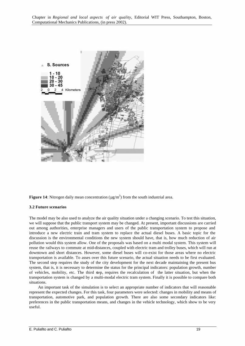
3.1 Model outputs After the calibration process has concluded, it is possible to study the spatial distribution of the ambient concentration for the entire city. As an example of these model outputs, two years (1997-98) of meteorological data, has been calculated. Different temporal integration are possible, but normally, the following averaging conditions are usually computed: maximum hourly values, 24 h, 30 days, and annual mean values. The next figures show several types of outputs, which illustrates the calculated conditions. Figure 9 shows a map with the spatial distribution of the street hierarchies and figure 10 displays the respective average traffic flow for each street. Based in this information, it is possible to establish a pollutant emission inventory for the mobile sources. Figure 11 plots, for example, the emission pattern for NOx. Figure 12 shows the calculated ambient concentration for NOx produced by the mobile sources, where it is possible to recognize areas with a mayor impact on the air quality, especially close to the central business area. As examples of the industrial areas, figure 13 shows the influence of the Refinery located south of the city as the main source of SO2, reaching maximum hourly values at the urban areas of the city of 100 µg/m3, and more than 400 µg/m3 in areas close to the source. Most of it is vented through the torch, although lately the refinery has incorporated a desulphuration Claus plant to reduce their SO2 emissions. At the south industrial area, the ferrous alloy and the coal burning processes are the main emitter, especially because they function with out any filtering device to their dust emissions. Maximum hourly immission values may reach 1500 µg/m3 and more than 200 µg/m3 daily mean values close to the sources. Ten kilometers away, at a residential part of the city annual mean values of 30 to 40 µg/m3 can be obtained, especially during the winter months. According to the calculations and the monitoring measurements, the influence of the industrial sources over the city do not exceed the air quality standard, with the exception of areas close to the industrial area. The power plant at Lujan de Cuyo is the main NOx emitter, but the concentration values do not exceed the local standard (100 µg/m3 for 1 year and 200 µg/m3 for 24 h). Mean daily values reaches de 20 to 40 µg/m3 and annual mean do not exceed 5 to 10 µg/m3, due to industrial sources. NOx values at the urban areas are mainly produced by vehicle exhaust. Figure 14 show a daily mean concentration map of nitrogen oxides emitted from the southern industrial area.



Figure 9: Street hierarchies for the Mendoza metropolitan area.



Figure 10: Average traffic flow in the city metropolitan area.



Figure 11: Emission pattern for mobile sources in Mendoza.



Figure 12: Ambient concentration values of NOx (µg/m3) produced by the road vehicles in Mendoza.



Figure 13: Annual average of 8 hr. Sulphur dioxide concentrations.



Figure 14: Nitrogen daily mean concentration (µg/m3) from the south industrial area.

3.2 Future scenarios The model may be also used to analyze the air quality situation under a changing scenario. To test this situation, we will suppose that the public transport system may be changed. At present, important discussions are carried out among authorities, enterprise managers and users of the public transportation system to propose and introduce a new electric train and tram system to replace the actual diesel buses. A basic topic for the discussion is the environmental conditions the new system should have, that is, how much reduction of air pollution would this system allow. One of the proposals was based on a multi modal system. This system will reuse the railways to commute at mid-distances, coupled with electric tram and trolley buses, which will run at downtown and short distances. However, some diesel buses will co-exist for those areas where no electric transportation is available. To asses over this future scenario, the actual situation needs to be first evaluated. The second step requires the study of the city development for the next decade maintaining the present bus system, that is, it is necessary to determine the status for the principal indicators: population growth, number of vehicles, mobility, etc. The third step, requires the recalculation of the latter situation, but when the transportation system is changed by a multi-modal electric tram system. Finally it is possible to compare both situations. An important task of the simulation is to select an appropriate number of indicators that will reasonable represent the expected changes. For this task, four parameters were selected: changes in mobility and means of transportation, automotive park, and population growth. There are also some secondary indicators like: preferences in the public transportation means, and changes in the vehicle technology, which show to be very useful.



From the source and destiny survey of 1998, it is known that 1,400,000 trips are performed daily within the metropolitan area. Public diesel buses carry around 510,000 passengers daily, implying 35% of the daily trips, while other 610,000 trips (45% of the daily trips) are done in private cars. However, the ratio public-to-private transportation is decreasing, showing a preference in using the own car. Table 2 records the main parameters and indicators used to estimate years 1999 and 2010. Analyzing the present trend, it is expected a 5% yearly increase in new vehicles, with a 1,5% yearly dismiss. With these values, it is possible also to estimate the actual vehicle technology and also to approximate the variation of the emission factors. In Table 3 we summarize the expected emission factors for year 2010, considering the estimated composition of the on road vehicles. It is foreseen, a reduction in the emission factors for 2010, due to technological improvement, however the impact of these improvements are weighted by the age of the older fleet.

Table 2: Number of daily trips vs. means of transportation.

Year 1999 2010 Means of transportation No. Of

Trips Relative % No. Of Trips

Public diesel bus 493600 34.9% 623100 Trolley bus 14900 1.1% 18800 Contracted (diesel) bus 5900 0.4% 7500 School bus 13400 0.9% 16900 Taxi or remise 23000 1.6% 29000 Own car, as driver 354700 25.1% 447800 Car, as accompanying 201000 14.2% 253700 Motorcycle 35200 2.5% 44400 Bicycle 102700 7.2% 129600 Walking more than 1000 m 111200 7.9% 140300 Other means (not specified) 59700 4.2% 75400 Total 1415300 100.0% 1786500

Table 3: Principal indicators for 1999 and 2010.

Year 1999 2010 Population (inhabitants) 895000 1050000 Mobility (number of daily trips per inhabitants) 1.58 1.7 Growth in the number of trips (1999-2010) 1.26 Population growth rate (1999-2010) 1.21 Private vehicle growth rate 1999-2010 1.36 Motorization rate (inhabitants per car) 3.1 2.7 Passengers per private car (per trip) 1.45 1.50 Number of private vehicles 291000 381000

As important parameter scenario for year 2010, we considered 25% of private car users using public transportation and a second scenario with only ten percent of car users switching to the electric system. Under these bases, daily traffic, emissions and ambient concentration values for air pollutants were estimated.

3.3 Results of the simulation Once the scenario is chosen, the principal calculations are the geographical distribution of daily traffic flow, emissions and ambient values for air pollutants. Normal output for this model are: a) daily vehicle fluxes, b) daily mean emission for TSP: Total suspended particles, NOx: Nitrogen oxides, HC: hydrocarbons and CO Carbon monoxide; c) total emissions for given areas of the city, discriminated according to the vehicle type and fuel; d) expected immissions for the present situation (1999), for year 2010 under several scenarios and for year 2010 incorporating the electric tram system. The total daily emissions for the city, for an approximate area of 25 x 20 km, can be calculated as a function of the type fuel consumption, which can also be interpreted in terms of private (mainly gasoline) and



public (mainly diesel) transport. This information is displayed in Table 4, while Table 5 shows these data as a ratio of emission to transported passengers. These two tables clearly remark that the public transport has a better overall performance than private cars, considering total daily emissions. Only for particles (total mass) diesel buses are worst than the gasoline vehicles.

Table 4: Daily emission of pollutants by fuel type in kg for year 1999.

Emission (in kg) / Transport mode Public (diesel) Private (gasoline) Total suspended particles (TSP) 600 400 Nitrogen (NOx) 850 2500 Hydrocarbons (HC) 950 2900 Carbon monoxide (CO) 5250 18400

Table 5: Ratio of the daily emissions to carried passengers for year 1999.

Emission per passenger (in g/pass.) Public (diesel) Private (gasoline) Total suspended particles (TSP) 1.15 0.60 Nitrogen (NOx) 1.65 3.65 Hydrocarbons (HC) 1.80 4.25 Carbon monoxide (CO) 10.25 26.65

Table 6 shows a comparison of the estimated total mean daily emission of the city, calculated for: a) year 1999; b) year 2010, no change (NP); and c) year 2010 with the proposed tram system on going (WP). It is foreseen for year 2010 an increase in air pollutant emissions from 20 to 40%, under the scenario presented in Tables 2 and 3. Consequently a worsening of the air quality is expected, both in absolute concentration values as well as an extension of the affected area. As an example, figure 15 (a) shows the calculated suspended particle concentrations for year 2010 and figure 15 (b) plots how the area with critical ambient concentration values could be reduced in extension and in absolute values, when the expected tram project is carried out. A higher positive impact is expected on Carbon monoxide and hydrocarbons emissions, because of their non linear dependence with the vehicle velocity. This double effect will improve or at least stabilize the present air quality in the city, despite the expected population and traffic growth. As traffic density increases, lower speeds are developed and hence producing higher emissions. On the contrary, as more users prefer a clean and safe electric public transport, traffic intensity will diminish considerably, and higher regular speeds can be achieved for those who use private transportation.

Table 6: Total daily emission of pollutants by mobile sources in tons.

Contaminant (in tons) 1999 2010 (NP) 2010 (WP) Total suspended particles (TSP) 1 1.4 1.0 Nitrogen (NOx) 3.4 4.3 3.2 Hydrocarbons (HC) 3.9 4.7 2.7 Carbon monoxide (CO) 23.6 30.3 18.0



Figure 15: Calculated Suspended particles (µg/m3) for year 2010, with present diesel public bus system (NP)

and under the projected electric public system scenario (WP).

4. Case study In the early morning of May 15, 1995, the population of the city of Mendoza was affected by a high pollution event, which produced serious pulmonary affections. During several hours hundreds of persons, especially children, needed to be hospitalized. Since no Enterprise or Company claimed to be the responsible for such situation, our Institute for Environmental research was called by the Federal Justice to study the case and to produce an environmental assessment. To study this case, we followed three lines of action: 1) we performed a epidemiological survey on the symptoms of the affected persons to see what kind of pollutant could be the responsible; 2) We collected the meteorological data and, according to the suspected pollutant, we run a dispersion model for possible emissions; 3) We tested the dispersion model with continuous monitoring measurements. Finally the federal judge as an important proof for the respective investigation and trial used our written assessment.

4.1 Epidemiological survey The main symptoms were associated in two groups: a) respiratory affections and dyspnea; b) headache, migraine, nausea and vomits. According to the patients, the event had a duration between two and four hours. Given also the strong smell witnesses by the affected persons and the intensity of the respiratory affections, we preliminary concluded that it could be a combination of Sulphur oxides and hydrogen Sulphur (SO2 and H2S) in presence of particulate matter (Folinsbee [14]; Pönkä [15]; Mustafa [16]). The reached ambient concentration of the gases could approximately be between 0.05 and 1 ppm. Note that the lower olfactory threshold of H2S is approx. 0.025-0.05 ppm. Unfortunately there were no SO2 or H2S measurements available that day.

4.2 Meteorological conditions During the first hours of May, 18, the meteorological conditions were: cold, calm winds (less than 1.5 m/s) from SW, overcastted with high pressure, characterized as stable with low inversion layer less than 200 - 300 m. By the midday the conditions improved to convective with soft winds.

4.3 Dispersion models Given the meteorological conditions and the intensity of the epidemiological aspects, only few possible stationary sources could be responsible of the emission. We simulated a short high emission from the



Refinery located 16 km SW from the affected area of the city. Supposing a worst-case scenario, with 500 kg/h of sour gases emitted at an 80 m high stack, and considering that 10 km downwind we may have had at least 10 % of H2S and 90 % of SO2, we obtained: Conc. SO2 = 2830 (µg / m3). 0,9 = 2547 (µg / m3) = 1,14 ppm Conc. H2S = 2830 (µg / m3). 0,1 = 283 (µg / m3). = 0,24 ppm Which confirms that our first guess on possible concentrations could have been possible.

4.4 Monitoring measurements As said before, there were no SO2 or H2S measurements available during this episode. But at our Institute IEMA we monitored surface ozone, detecting an anomalous situation. The monitoring station is located around 16 km SW downwind from the Refinery, and is closed to the affected area. We study how O3 could be affected by H2S, concluding that, after neglecting other smog components, the following reaction could take place [10]:

H2S + O3 →H2O + SO2 (5) Considering that the reaction time of 1 ppb of H2S in presence of 50 ppb of O3 with 15 000 particles / cm3 is about 2 hours. Then the dynamic variation of the ozone concentration may be expressed by:

[ ] [ ] [ ]O O t e e

d OdT

e d TM M K t K t

E

t

t K T3 3 0

31 1

0

1= +− − ∫( ) ( ) ( ) ( ) (6)

where [ ]K t k H S dTrt

t

1 20

( ) = ∫ and [ ]K T k H S d Trt

T

1 20

( ) '= ∫

[O3]M is the measured concentration for any t, [O3]M (t0) is the initial value, and [O3]E is the due value if [H2S] were not present. t0: initial time, t1 is end time of the reaction, kr reaction rate for H2S de 1,11x10-5 [ppb-1 seg-

1], for T= de 25 C (289,15 K); krT: reaction temperature dependence T0= 0 C (273,15 K) and α= 15; τ: reaction time rate, approx. 30 min, [H2S]: Hydrogen Sulphur concentration.

4.5 Results of the simulation model The resolution of the continuity equation yields in a Hydrogen Sulphur [H2S] pulse as it can be seen in figure 16. The [H2S] concentration, which is represented in continuous line, is the input in our program that reproduces the measurement of May 18. The mean square root of the olfactory threshold (50 ppb) is drawn in dotted line. This pulse begins approximately at 8:00 a.m. with a wave front of 100 ppb. This curve surpasses the olfactory threshold nearly some time before 9:00 a.m., and around 12:30 p.m. the smell is not perceived any more. The next figure 17 shows with pointed line the average value of ozone for May [O3]E(t), this value represents the expected value of ozone if the H2S pulse were not present. The continuous line is the true measured ozone value for May 18 [O3]M (t). The dashed line represents the simulation value [O3]C(t). Finally, the point-dashed line represents the measured value; compare this curve with the measured value. The value measured on May 18 had a different feature compared to ozone values of many days with similar meteorological characteristics, which gave a strong evidence of the presence of a anomalous situation. This could not been explained only by the presence of typical smog situation. The strong decay measured between 11:30 am and 12:00 pm gave us an indication of the reaction time of equation (6).



Figure 16: Emission of Hydrogen Sulphur H2S during a pollution episode in May 18, 1995.

4.6 Conclusions of the case study Using dispersion models and solving the temporal variation of ozone measured at the Institute, we calculated approximately the presence of SO2 and a H2S pulse of at least 100 ppb during 4 hours. Moreover, the epidemiological studies of the affected population also concluded that the presence of SO2 and H2S, in the same order of magnitude as it was calculated, could produce the detected respiratory affections. Several years later, during the trial process, personnel of the Refinery declared that due to a wrong maneuver, sour gases where vented through a secondary torch tower and emitted to the atmosphere with out burning it. The lapse time of the event and the amount of gases emitted where approximately the same as calculated.

Figure 17: Reconstructed ozone concentrations at Benegas during May 18, 1995. O3 Measurements

(continuous dark line), expected ozone values if the H2S pulse of figure 16 were not present (dotted line with X), simulated ozone concentrations (gray line).

As a consequence of this event, the Refinery incorporated a Claus plant that treats more than 95% of the produced sour gases and only occasionally they are vented directly through the torch to the atmosphere.



5 Conclusions The city of Mendoza has implemented a vast environmental program. This program includes various technical and legal aspects such as: a) environmental information; b) legal, and economic instruments for environmental protection; c) development of public environmental awareness; d) natural flora and fauna preservation; e) environmental control and sanitation; f) urban regulation and development; etc. An important task of an air quality management system is to establish suitable air quality targets; and to determine how effective these targets are temporally and geographically complied. Another important aspect is to forecast the possibility to reduce pollution emissions. Such an air quality system has three important components: monitoring of main pollutants; realization of a comprehensive model, and development of satisfactory legal strategies. This articles emphasizes the modeling efforts. The implemented model is based on a Geographical Information System, which offers various advantages to handle spatial and temporal data. GIS combines data with algorithms, procedures and models that represent general scientific understanding. In this article we showed the actual air quality situation in the city and we presented also possible future scenarios. Finally we have presented a high pollution episode occurred in the city, where many persons suffered respiratory affections. The modeling of this event was very useful to determine the legal responsibilities and to enforce the proper abatement strategies.

6 Acknowledgements The authors would like to thank the authorities of the University of Mendoza for the support to the research activities. Also are here acknowledged the engineers and technicians of our Institute IEMA for the permanent work in taking the daily measurements and calibrating the equipments. We thank as well the Ministry of Environment and Public Works of the Province of Mendoza, for permitting the use of the data from the monitoring stations. Our gratitude to the German colleagues from the Max Planck Institut für Aeronomie Lindau, in the person of Prof. Dr. Gerd Hartmann and the Center for Environmental Research in Leipzig, represented by Prof. Dr. Olf Herbarth and Dr. Ludwig Weißflog for their friendly and fructuous cooperation. This study was partially funded by Argentine-German International Scientific Cooperation and the Argentine Agency for Science and Technology (FONCYT) under grant PICT97 N° 13-00000-01579. We are also grateful to WIT Press for the kind invitation to present this article.

7 References [1] Schlink, U., Puliafito, E., Herbarth, O., Puliafito, J.L., Richter, M., Puliafito, C., Quero, J., Endlicher, W.,

Zahnen, B. Ozone air Pollution in Mendoza. in Air Pollution VI, Serie Advances in Air Pollution, Brebbia C., Ratto C., Power H. (Eds.), Witt Press, pp 435-444, 1998.

[2] Schlink, U, Herbarth, O., Richter, M., Rhewagen, M., Puliafito, J.L., Puliafito, E., Puliafito, C., Guerreiro, P., Quero, J.L., Behler, J.C. Ozone-Monitoring in Mendoza, Argentina: Initial results. J. Air and Waste Management Assoc. 49, 82-87, 1999.

[3] Puliafito E., Puliafito, J.L., Behler J.C, Alonso, P. La calidad del aire en Mendoza: Contaminación y efectos sobre la salud. In Mendoza Ambiental, Martinez, E. and Dalmasso, A., (Eds.), pp. 207-242, Mendoza, Argentina. ISBN 950-43-7961-6, 1995.

[4] Weißflog, L., Paladini, E., Gantuz, M., Puliafito, J., Puliafito, S., Wenzel, K., Schüürmann, G. Immission patterns of airborne pollutants in Argentina and Germany. I. First results of a heavy metal biomonitoring. Fresenius Environm. Bullet. (3) 728-7233.

[5] Wenzel, K., Weißflog, L., Paladini, E., Gantuz, M., Guerreiro, P., Puliafito, C., Schüürmann G. Immission patterns of airborne pollutants in Argentina and Germany. II. Biomonitoring of organo chlorine compounds and polyciclic aromatics. Chemosphere 34, pp 2505-2518, 1997.

[6] Puliafito, J.L: A South American Country Example: Environmental legislation Enforcement in Mendoza; Experience and challenges. Proc. of the Third International Conference on Environmental Enforcement, Vol. 2, pp51-62, Oxaca México, April 25-28, Gerardu, J., Wesserman, C., USEPA and Ministry of Housing and Spatial Planning and Environment (VROM) the Nederlands; VROM8300/133, 1994.

[7] Herbarth, O., Fritz, G., Behler, J.C., Rehwagen, M., Puliafito, J.L., Richter, M, Schlink, U., Sernaglia, J., Puliafito, E., Puliafito, C., Schilde, M., Wildführ, W. Epidemiologic Risk analysis of environmentally



attributed exposure on airway diseases and allergies in children. Centr. Eur. J. Publ. Health 7, (2), pp 72-76, 1999.

[8] Herbarth, O., Fritz, G., Wildfür, W., Behler, J.C. An epidemiological study to the effects of traffic and domestic heating attributed emissions on respiratory illness and allergies among children, Epidemiology, 7(4),86, 1996.

[9] Zanetti, P. Air pollution modeling. Computational Mechanics Publications, Southampton Boston. Van Nostrand Reinhold, New York, 1990.

[10] Seinfeld, J. Air pollution, physical and chemical fundamentals. McGraw-HilL, NewYork. 1975. [11] CONCAWE Reports: Motor vehicle emission regulations fuel specifications, Part 1, summary and annual

1996 update. Reports, No. 5/97, 1997. [12] Andrias, A., Samaras, Z., Zafiris, D., Ziercok, K. CORNAIR Working Group on emission factors for

calculating 1990 emission form road traffic. Final report, Document of the European Commission ISBN 92-826-5572-X,1993.

[13] Hoydish, G., Dabbert, F. Kinematics and dispersion characteristics of flows in asymmetric street canyons. Atmospheric Environment, 22, 2677-2689,1988.

[14] Folinsbee, L.: Human Health Effects of Air Pollution, Env. Health Perspectives, Vol 100, pp 45-56, 1993.

[15] Pönkä, A, A. Virtaten: Chronic Bronchitis, Emphysema, and Low-Level Air Pollution in Helsinki, 1987-1989. Environmental Research 65, 207-217, 1994.

[16] Mustafa, M., D. Tierney: Biochemical and Metabolic Changes in the Lung with Oxygen, Ozone, and Nitrogen Dioxide Toxicity, American Review of Respiratory Disease, Vol. 118, 1978.

Documents

Monitoring and modeling air quality in Mendoza, Argentinalidecc.cs.uns.edu.ar/~nbb/ccm/downloads/Clases/Literatura/EP... · desert climate and to improve urban ... the region is characterized