University of Northern Iowa University of Northern Iowa

UNI ScholarWorks UNI ScholarWorks

Honors Program Theses Honors Program

2018

Money matters: An analysis of campaign finance in United States Money matters: An analysis of campaign finance in United States

House of Representatives elections, 2010-2016 House of Representatives elections, 2010-2016

Destiny Leitz University of Northern Iowa

Let us know how access to this document benefits you

Copyright ©2018 Destiny Leitz

Follow this and additional works at: https://scholarworks.uni.edu/hpt

Part of the American Politics Commons, and the Applied Mathematics Commons

Recommended Citation Recommended Citation Leitz, Destiny, "Money matters: An analysis of campaign finance in United States House of Representatives elections, 2010-2016" (2018). Honors Program Theses. 328. https://scholarworks.uni.edu/hpt/328

This Open Access Honors Program Thesis is brought to you for free and open access by the Honors Program at UNI ScholarWorks. It has been accepted for inclusion in Honors Program Theses by an authorized administrator of UNI ScholarWorks. For more information, please contact scholarworks@uni.edu.

MONEY MATTERS

MONEY MATTERS: AN ANALYSIS OF CAMPAIGN FINANCE IN

UNITED STATES HOUSE OF REPRESENTATIVES ELECTIONS, 2010-2016

A Thesis Submitted

in Partial Fulfillment

of the Requirements for the Designation

University Honors

Destiny Leitz

University of Northern Iowa

May 2018

MONEY MATTERS

This Study by: Destiny Leitz Entitled: Money Matters: An Analysis of Campaign Finance in United States House of Representatives Elections, 2010-2016 has been approved as meeting the thesis or project requirement for the Designation University Honors ________ ______________________________________________________ Date

Mark Ecker, Honors Thesis Advisor, Department of Mathematics

________ ______________________________________________________ Date Dr. Jessica Moon, Director, University Honors Program

MONEY MATTERS 1

Introduction

Money in politics is the single largest threat to the democratic system in the United States.

It influences everything in politics, from the candidates to the issues debated. Every American

knows that running for office requires large amounts of funding, and being elected requires even

more. People worry that only the wealthiest voices are being heard; of course, candidates who

depend on money from wealthy donors for campaign strength would never support unfavorable

policies for their donors. Clearly, money in politics threatens the core democratic principles upon

which America was founded. However, few people discuss whether the money really makes a

difference in elections, and much of the outstanding literature on the impact of campaign funding

on election results dates back over twenty years. To make things worse, each study uses different

methodologies, so their results are difficult to compare. Since these studies were published, the

way that candidates finance their campaigns has completely changed. The Citizens United decision

in 2010 allowed corporations and political action committees, or PACs, to play a major role in

campaign funding. Still, funding is a strong predictor of election outcomes; a large amount of funds

indicates campaign strength for challengers but campaign weakness for incumbents. The impact

of campaign finance can depend on the source of funding. Incumbents tend to gain most from

individual donations, while challengers gain the most from PAC donations. Without serious

consideration of campaign finance reform, money will continue to be the primary source of

campaign strength and the wealthy will continue to influence elections.

Literature Review

Influence of Campaign Funding on Election Outcomes

Previous literature focused on the relative impacts of incumbents’ and challengers’

spending. As a challenger increased her campaign spending, the better she did in elections. Not

MONEY MATTERS 2

only did her average vote increase, but the frequency of challenger victories grew (Jacobson, 1978,

1990, 2006). One possible explanation is that in order to gather voter support, the candidate must

first become familiar to the voters. Then on Election Day, voters select candidates whom they

recognize. Spending campaign funds on advertising and other modes of marketing increases the

probability that a voter will become familiar with a particular campaign and will subsequently

support that candidate. McBurnett and McBurnett (1994) investigated which subsets of the

population were more likely to be swayed by campaign spending. They observed that people with

college degrees, people with an interest in political campaigns, and strong partisans were the least

likely to be affected.

Incumbents have a distinct outlook on campaign expenditures because they enjoy what

Jacobson (1978, 470) termed an “incumbency advantage.” Because they should already be familiar

to voters, incumbents do not need to spend as much campaign money to become recognized by

voters (Glantz, Abramowitz, & Burkhart, 1976; Silberman, 1976; Grier, 1989; Jacobson, 1990;

Abramowitz, 1991). Jacobson (1990) argued that voters will not turn against an incumbent without

a viable replacement. Therefore, it has been shown that if an incumbent is required to spend large

sums of money, they are less likely to be reelected -- not because their spending deters voters, but

because they only spend excessively when a formidable challenger presents herself. In this way,

incumbent spending is purely reactionary to challenger spending (Jacobson, 1978; Glantz et al.,

1976). Ironically, this spending does little, if anything, to improve election prospects (Caldeira &

Patterson, 1982; Jacobson, 1990; Levitt, 1994).

The campaigning period is crucial for challengers, especially, to reach voters with their

message. Several studies found that as a challenger’s expected vote count rose, their funding also

rose (Jacobson, 1978, 1985, 2006; Giertz & Sullivan, 1977). After all, contributors are more likely

MONEY MATTERS 3

to raise funds for candidates they support. As a candidate garners additional supporters, these

supporters will raise additional funding for the candidate. Therefore, it is difficult to determine a

cause and effect relationship between candidate success and funding. In other words, strong

candidates are able to gain funding, but funding also leads to winning elections. In statistics, this

problem is called confounding bias, otherwise known as simultaneity bias. Because the

expectations of election results cannot be modeled perfectly, the effect of challenger spending is

often overstated while the effect of incumbent spending is understated.

Previous researchers tackled simultaneity bias in several ways. The first is by eliminating

the variable for candidate funding altogether. Instead, they used the opponent’s campaign

expenditures to explain movement in voter support (Giertz & Sullivan, 1977). As a result, they

were able to remove the influence that a candidate’s spending had on their own voting, thereby

eradicating simultaneity bias. Other researchers used other functional forms, such as two-stage

least squares regression, in an attempt to define the cause and effect relationship between the two

variables (Jacobson, 1985). Grier (1989) denounced simultaneity bias altogether by arguing that if

campaign contributions are strictly based on expected candidate strength, then losing candidates

should be known from the beginning of the campaign cycle and will not be able to attract any

funds at all. However, that is not the case, since many losing candidates in past elections were able

to adequately finance their campaigns. Due to a lack of standardization between these methods,

the existing studies on the relative impact of incumbent and challenger spending on election results

have been inconclusive.

The results set forth by these past investigations have had major government policy

implications. First, because challengers are highly dependent on campaign funding to attract votes,

any government restrictions that limit campaign contributions will favor incumbents. Therefore, it

MONEY MATTERS 4

is no surprise that Congressmen do not vote to eliminate spending limit laws (Glantz, Abramowitz,

& Burkhart 1976; Abramowitz, 1991). The problem is exacerbated by the fact that incumbents

receive fewer individual contributions than challengers, and that their contributions are smaller in

size (Grier, 1989). Therefore, incumbents do not face the risk of losing funding if contribution

limits are enacted.

The Role of PACs and SuperPACs

Political action committees, commonly known as PACs, have long played a role in

campaign finance and election outcomes. These interest groups, who raise and contribute money

to campaigns of candidates likely to support their ideology, were introduced in 1944. While PACs

generally represent businesses, labor unions, or ideological interests, the process to create one is

not restricted to these groups. PACs are currently limited to a $5,000 donation to a single candidate

per election period, and $15,000 to a national party committee each year (The Center for

Responsive Politics, n.d.). PACs generally focus their contributions on incumbents (Giertz &

Sullivan, 1977; Welch, 1980). This suggests that PACs are more interested in gaining political

favors than influencing elections. In other words, they devote their money to candidates who

support their platform and have demonstrated an ability to win the election and advocate for their

ideas. After all, money given to the loser will be wasted, since she will not be able to affect the

legislature in the PAC’s favor.

Since these relationships were investigated, several court cases have reformed the world of

campaign finance. A landmark court decision regarding PACs was delivered by Citizens United v.

Federal Election Commission (2010). The Supreme Court ruled that limits on corporate funding

of independent political broadcasts in elections violate the First Amendment. This case is infamous

for addressing corporate personhood, in that they hold the same First Amendment rights as

MONEY MATTERS 5

citizens. Just months after the Citizens United decision, SpeechNow.Org v. Federal Election

Commission (2010) asserted that contribution limits on other groups and individuals were

unconstitutional as well, following the same logic as Citizens United.

More recent literature has investigated how the Citizens United decision has affected the

incumbency advantage. Jacobsen (2014) argued that growing party loyalty has diminished this

advantage in recent years. Fewer people are willing to vote for the opposite party, regardless of

the incumbency status of the candidates. Therefore, incumbents are increasingly campaigning in

districts where their challengers’ parties are favored. With more money available to them,

especially in districts that lean toward their party, challengers are able to respond to the

incumbents’ campaigns more effectively.

Citizens United has also had major implications on how campaigns are funded. In the

aftermath of these court decisions, the Federal Election Commission reported a nearly 470%

increase in independent expenditures by PACs, groups, and individuals (Bauerly, 2011).

Specifically, PAC funding doubled between the 2008 and 2010 elections, and accounted for more

than individuals, corporations, and unions combined. More importantly, the SuperPAC was born.

These organizations raise unlimited sums of money from businesses, unions, and individuals to

advocate for or against candidates, but cannot donate directly to the candidate’s campaign. Because

PACs are not required to disclose the sources of their funding, corporations and the wealthiest

Americans are able to donate immense funds to support candidates who support favorable policies.

Thus, the issue of PACs, especially SuperPACs, is hotly debated. However, it has yet to be

determined whether these expenditures truly help a candidate secure a victory.

MONEY MATTERS 6

Methodology

Incumbent Votes Earned

To analyze the impact of campaign finance on the percentage of votes garnered by the

incumbent, a multivariate ordinary least squares (OLS) regression model was employed:

𝐼𝑛𝑐𝑉𝑜𝑡𝑒% = 𝛽0 + 𝛽1 𝐼𝑛𝑐𝑅2010 + 𝛽2 𝐼𝑛𝑐𝑅2012 + 𝛽3 𝐼𝑛𝑐𝑅2014

+ 𝛽4 𝐼𝑛𝑐𝑅2016 + 𝛽5 𝐿𝑛(𝑇𝑜𝑡𝐼𝑛𝑐) + 𝛽6 𝐿𝑛(𝑇𝑜𝑡𝐶ℎ𝑎𝑙𝑙)

+ 𝛽7 𝐿𝑛(𝐼𝑛𝑑𝐼𝑛𝑐) + 𝛽8 𝐿𝑛(𝐶𝑜𝑚𝑚𝐼𝑛𝑐) + 𝛽9 𝐿𝑛(𝐶𝑎𝑛𝑑𝐼𝑛𝑐)

+ 𝛽10 𝐿𝑛(𝐿𝑜𝑎𝑛𝐼𝑛𝑐) + 𝛽11 𝐿𝑛(𝑂𝑡ℎ𝑒𝑟𝐼𝑛𝑐) + 𝛽12 𝐿𝑛(𝐼𝑛𝑑𝐶ℎ𝑎𝑙𝑙)

+ 𝛽13 𝐿𝑛(𝐶𝑜𝑚𝑚𝐶ℎ𝑎𝑙𝑙) + 𝛽14 𝐿𝑛(𝐶𝑎𝑛𝑑𝐶ℎ𝑎𝑙𝑙)

+ 𝛽15 𝐿𝑛(𝐿𝑜𝑎𝑛𝐶ℎ𝑎𝑙𝑙) + 𝛽16 𝐿𝑛(𝑂𝑡ℎ𝑒𝑟𝐶ℎ𝑎𝑙𝑙) + 𝜀

(1)

The dependent variable, IncVote% is the percentage of the vote earned by the incumbent.

IncR2010, IncR2012, IncR2014, and IncR2016 are binary variables, which equal 1 if the incumbent

was a Republican in the given election year, and zero otherwise. These variables capture whether

a particular party was favored in any of the elections.

The next two variables, Ln(TotInc) and Ln(TotChall) measure the log-scaled total funding

received by the incumbent and challenger, respectively. The incumbent’s share of the vote is

expected to rise when the incumbent’s spending rises or the challenger’s spending falls. A natural

logarithm transformation is appropriate because it captures the diminishing marginal utility of

funding. For example, a $1,000 donation is more valuable to a candidate with a $5,000 campaign

than a $5 billion campaign. This methodology is common practice among studies involving

monetary values.

The last ten variables categorize the contributions by source. Ln(IndInc) and Ln(IndChall)

contain the log-scaled contributions from individuals for incumbents and challengers, respectively.

MONEY MATTERS 7

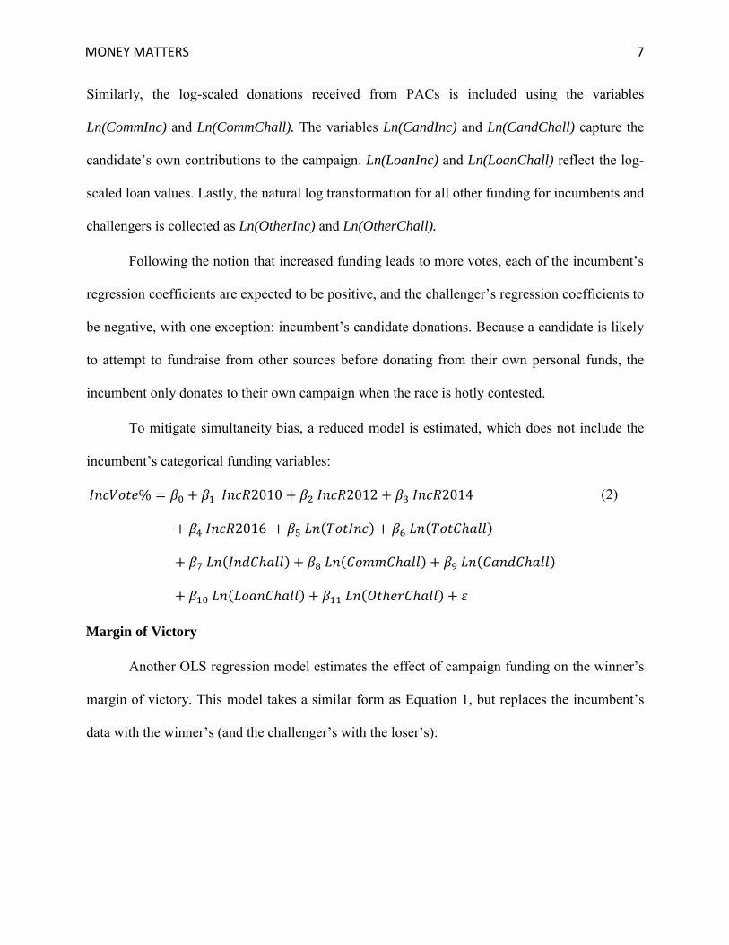
Similarly, the log-scaled donations received from PACs is included using the variables

Ln(CommInc) and Ln(CommChall). The variables Ln(CandInc) and Ln(CandChall) capture the

candidate’s own contributions to the campaign. Ln(LoanInc) and Ln(LoanChall) reflect the log-

scaled loan values. Lastly, the natural log transformation for all other funding for incumbents and

challengers is collected as Ln(OtherInc) and Ln(OtherChall).

Following the notion that increased funding leads to more votes, each of the incumbent’s

regression coefficients are expected to be positive, and the challenger’s regression coefficients to

be negative, with one exception: incumbent’s candidate donations. Because a candidate is likely

to attempt to fundraise from other sources before donating from their own personal funds, the

incumbent only donates to their own campaign when the race is hotly contested.

To mitigate simultaneity bias, a reduced model is estimated, which does not include the

incumbent’s categorical funding variables:

𝐼𝑛𝑐𝑉𝑜𝑡𝑒% = 𝛽0 + 𝛽1 𝐼𝑛𝑐𝑅2010 + 𝛽2 𝐼𝑛𝑐𝑅2012 + 𝛽3 𝐼𝑛𝑐𝑅2014

+ 𝛽4 𝐼𝑛𝑐𝑅2016 + 𝛽5 𝐿𝑛(𝑇𝑜𝑡𝐼𝑛𝑐) + 𝛽6 𝐿𝑛(𝑇𝑜𝑡𝐶ℎ𝑎𝑙𝑙)

+ 𝛽7 𝐿𝑛(𝐼𝑛𝑑𝐶ℎ𝑎𝑙𝑙) + 𝛽8 𝐿𝑛(𝐶𝑜𝑚𝑚𝐶ℎ𝑎𝑙𝑙) + 𝛽9 𝐿𝑛(𝐶𝑎𝑛𝑑𝐶ℎ𝑎𝑙𝑙)

+ 𝛽10 𝐿𝑛(𝐿𝑜𝑎𝑛𝐶ℎ𝑎𝑙𝑙) + 𝛽11 𝐿𝑛(𝑂𝑡ℎ𝑒𝑟𝐶ℎ𝑎𝑙𝑙) + 𝜀

(2)

Margin of Victory

Another OLS regression model estimates the effect of campaign funding on the winner’s

margin of victory. This model takes a similar form as Equation 1, but replaces the incumbent’s

data with the winner’s (and the challenger’s with the loser’s):

MONEY MATTERS 8

𝑀𝑂𝑉 = 𝛽0 + 𝛽1 𝑊𝑖𝑛𝑅2010 + 𝛽2 𝑊𝑖𝑛𝑅2012 + 𝛽3 𝑊𝑖𝑛𝑅2014

+ 𝛽4 𝑊𝑖𝑛𝑅2016 + 𝛽5 𝑊𝑖𝑛𝐼𝑛𝑐 + 𝛽6 𝐿𝑛(𝑇𝑜𝑡𝑊𝑖𝑛)

+ 𝛽7 𝐿𝑛(𝑇𝑜𝑡𝐿𝑜𝑠𝑒) + 𝛽8 𝐿𝑛(𝐼𝑛𝑑𝑊𝑖𝑛) + 𝛽9 𝐿𝑛(𝐶𝑜𝑚𝑚𝑊𝑖𝑛)

+ 𝛽10 𝐿𝑛(𝐶𝑎𝑛𝑑𝑊𝑖𝑛) + 𝛽11 𝐿𝑛(𝐿𝑜𝑎𝑛𝑊𝑖𝑛) + 𝛽12 𝐿𝑛(𝑂𝑡ℎ𝑒𝑟𝑊𝑖𝑛)

+ 𝛽13 𝐿𝑛(𝐼𝑛𝑑𝐿𝑜𝑠𝑒) + 𝛽14 𝐿𝑛(𝐶𝑜𝑚𝑚𝐿𝑜𝑠𝑒) + 𝛽15 𝐿𝑛(𝐶𝑎𝑛𝑑𝐿𝑜𝑠𝑒)

+ 𝛽16 𝐿𝑛(𝐿𝑜𝑎𝑛𝐿𝑜𝑠𝑒) + 𝛽17 𝐿𝑛(𝑂𝑡ℎ𝑒𝑟𝐿𝑜𝑠𝑒) + 𝜀

(3)

Here, the dependent variable, MOV, is the margin of victory, which is calculated as the

difference in the percentage of the votes earned by the winner and the loser. One additional

independent variable is included in the study: WinInc, which is a binary variable equal to 1 if the

winner is the incumbent. Because incumbents enjoy an incumbency advantage, the associated

regression coefficient is anticipated to be positive. The other regression coefficients in this

equation are expected to have the same signs as in Equation 1.

Analogous to Equation 2, the model given in Equation 3 is reduced by removing the

winner’s categorical funding to mitigate simultaneity bias. This model is as follows:

𝑀𝑂𝑉 = 𝛽0 + 𝛽1 𝑊𝑖𝑛𝑅2010 + 𝛽2𝑊𝑖𝑛𝑅2012 + 𝛽3 𝑊𝑖𝑛𝑅2014

+ 𝛽4 𝑊𝑖𝑛𝑅2016 + 𝛽5 𝐿𝑛(𝑇𝑜𝑡𝑊𝑖𝑛) + 𝛽6 𝐿𝑛(𝑇𝑜𝑡𝐿𝑜𝑠𝑒)

+ 𝛽7 𝐿𝑛(𝐼𝑛𝑑𝐿𝑜𝑠𝑒) + 𝛽8 𝐿𝑛(𝐶𝑜𝑚𝑚𝐿𝑜𝑠𝑒) + 𝛽9 𝐿𝑛(𝐶𝑎𝑛𝑑𝐿𝑜𝑠𝑒)

+ 𝛽10 𝐿𝑛(𝐿𝑜𝑎𝑛𝐿𝑜𝑠𝑒) + 𝛽11 𝐿𝑛(𝑂𝑡ℎ𝑒𝑟𝐿𝑜𝑠𝑒) + 𝜀

(4)

Data

The data used in this study was collected from United States House of Representatives

elections from 2010 through 2016, which is available through the Federal Election Commission

(n.d.). All dollars were adjusted for inflation to 2016 dollars using the Consumer Price Index.

House of Representatives data was chosen because districts are drawn according to population.

MONEY MATTERS 9

Therefore, there was no need to adjust for population differences between elections. Because 2010

was the first election after the Citizens United decision, it serves as the first set of data. Data from

the 2016 election is the most recent available.

Several elections were omitted from this study. The data points for open seats and

uncontested races were discarded because the incumbency-challenger relationship is not present.

Furthermore, the FEC only requires reporting campaign finance data if $5,000 or more was raised

or spent by a candidate, though some candidates choose to do so even if this minimum is not met.

Therefore, only elections in which both the incumbent and the challenger reported campaign

finances are included in this study. Lastly, due to the small number of third-party candidates, only

elections between the two major parties (Democrat and Republican) are studied.

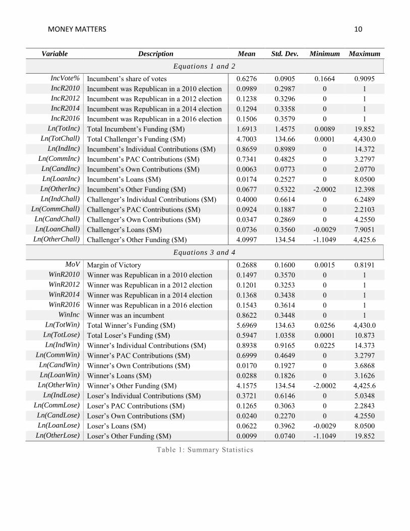
The final dataset includes 1,802 elections over the course of four election years. Summary

statistics can be found in Table 1. In the data, 86% of incumbents were reelected. The sample was

skewed towards Republicans, with 56% of them winning their election. Both of these rates

changed relatively little over the four election years. Surprisingly, the average spending by the

winner, loser, incumbent, and challenger also varied very little over the election years. It is

especially important to note that the average PAC spending did not change significantly over the

four election years. In this way, the Citizens United decision appears to have had little impact on

the role of PACs in campaign financing.

The 2012 election’s average spending is unrepresentative of the bulk of the data due to a

single election. In the state of Washington’s first district, Susan Delbene, a Democratic challenger,

spent $4.43 billion and won with 54% of the total vote. Because this figure is highly inflated

compared to the other elections, the average winner spending and average challenger spending are

MONEY MATTERS 10

Variable Description Mean Std. Dev. Minimum Maximum

Equations 1 and 2

IncVote% Incumbent’s share of votes 0.6276 0.0905 0.1664 0.9095 IncR2010 Incumbent was Republican in a 2010 election 0.0989 0.2987 0 1 IncR2012 Incumbent was Republican in a 2012 election 0.1238 0.3296 0 1 IncR2014 Incumbent was Republican in a 2014 election 0.1294 0.3358 0 1 IncR2016 Incumbent was Republican in a 2016 election 0.1506 0.3579 0 1

Ln(TotInc) Total Incumbent’s Funding ($M) 1.6913 1.4575 0.0089 19.852 Ln(TotChall) Total Challenger’s Funding ($M) 4.7003 134.66 0.0001 4,430.0

Ln(IndInc) Incumbent’s Individual Contributions ($M) 0.8659 0.8989 0 14.372 Ln(CommInc) Incumbent’s PAC Contributions ($M) 0.7341 0.4825 0 3.2797 Ln(CandInc) Incumbent’s Own Contributions ($M) 0.0063 0.0773 0 2.0770 Ln(LoanInc) Incumbent’s Loans ($M) 0.0174 0.2527 0 8.0500

Ln(OtherInc) Incumbent’s Other Funding ($M) 0.0677 0.5322 -2.0002 12.398 Ln(IndChall) Challenger’s Individual Contributions ($M) 0.4000 0.6614 0 6.2489

Ln(CommChall) Challenger’s PAC Contributions ($M) 0.0924 0.1887 0 2.2103 Ln(CandChall) Challenger’s Own Contributions ($M) 0.0347 0.2869 0 4.2550 Ln(LoanChall) Challenger’s Loans ($M) 0.0736 0.3560 -0.0029 7.9051

Ln(OtherChall) Challenger’s Other Funding ($M) 4.0997 134.54 -1.1049 4,425.6

Equations 3 and 4

MoV Margin of Victory 0.2688 0.1600 0.0015 0.8191 WinR2010 Winner was Republican in a 2010 election 0.1497 0.3570 0 1 WinR2012 Winner was Republican in a 2012 election 0.1201 0.3253 0 1 WinR2014 Winner was Republican in a 2014 election 0.1368 0.3438 0 1 WinR2016 Winner was Republican in a 2016 election 0.1543 0.3614 0 1

WinInc Winner was an incumbent 0.8622 0.3448 0 1 Ln(TotWin) Total Winner’s Funding ($M) 5.6969 134.63 0.0256 4,430.0

Ln(TotLose) Total Loser’s Funding ($M) 0.5947 1.0358 0.0001 10.873 Ln(IndWin) Winner’s Individual Contributions ($M) 0.8938 0.9165 0.0225 14.373

Ln(CommWin) Winner’s PAC Contributions ($M) 0.6999 0.4649 0 3.2797 Ln(CandWin) Winner’s Own Contributions ($M) 0.0170 0.1927 0 3.6868 Ln(LoanWin) Winner’s Loans ($M) 0.0288 0.1826 0 3.1626

Ln(OtherWin) Winner’s Other Funding ($M) 4.1575 134.54 -2.0002 4,425.6 Ln(IndLose) Loser’s Individual Contributions ($M) 0.3721 0.6146 0 5.0348

Ln(CommLose) Loser’s PAC Contributions ($M) 0.1265 0.3063 0 2.2843 Ln(CandLose) Loser’s Own Contributions ($M) 0.0240 0.2270 0 4.2550 Ln(LoanLose) Loser’s Loans ($M) 0.0622 0.3962 -0.0029 8.0500

Ln(OtherLose) Loser’s Other Funding ($M) 0.0099 0.0740 -1.1049 19.852

Table 1: Summary Statistics

MONEY MATTERS 11

highly skewed right. By removing Delbene’s election from the computation, the averages return

to values similar to the other three election years, as shown in Table 2.

Average Spending By Winner ($) Average Spending By Challenger ($)

Year N Including Delbene Excluding Delbene Including Delbene Excluding Delbene

2010 320 1,436,112 1,546,112 699,829 699,829 2012 227 21,190,353 1,682,346 20,095,784 582,934 2014 255 1,758,099 1,748,099 530,991 530,991 2016 280 1,853,555 1,853,555 588,060 588,060

Table 2: Average Spending by Election Year

Results

Prior to examining the regression results, it is important to understand statistical and

practical significance. Statistical significance is a measure of the meaningfulness or reliability of

the results. If a statistic is significant at the 10% level, then we are 90% sure that the results are

not due to chance. Therefore, the smaller the significance level, the stronger the evidence is.

Practical significance is somewhat different; it examines the magnitude of the result. If a statistic

is practically insignificant, it means that it has such a small effect that, even if it is statistically

significant, it is not useful in the real world. Meaningful statistics require both statistical and

practical significance. For example, if it is determined that campaign loans are strongly correlated

with the number of votes received, but getting millions of dollars of loans only improves the

number of votes by 1%, then the relationship is said to have statistical significance and practical

insignificance.

Incumbent Votes Earned

Table 3 presents the coefficients and statistical significance levels for Equation 1 and 2.

First, the Republican binary variables performed as expected. In 2010, Republicans swept the

MONEY MATTERS 12

Equation (1) (2)

Intercept 1.18618 1.22154 IncR2010 0.0254 *** 0.02616 *** IncR2012 -0.01102 * -0.01114 * IncR2014 0.01874 *** 0.01887 *** IncR2016 -0.00602 -0.00639

Ln(TotInc) -0.01332 ** -0.02370 *** Ln(TotChall) -0.01734 *** -0.01753 *** Ln(IndChall) -0.00203 -0.00196

Ln(CommChall) -0.00352 *** -0.00365 *** Ln(CandChall) 0.00037367 0.00044032 Ln(LoanChall) -0.00093493 ** -0.00099487 **

Ln(OtherChall) -0.00001507 -0.00011277 Ln(IndInc) -0.00554

Ln(CommInc) -0.00232

Ln(CandInc) -0.00131

Ln(LoanInc) -0.00093618

Ln(OtherInc) -0.00087694

R2 0.4666 0.4624 R2

adj 0.4586 0.4568

* Significant at 10% level | ** Significant at 5% level | *** Significant at 1% level

Table 3: Incumbent Vote Share Regression Results

MONEY MATTERS 13

United States House of Representatives elections, winning 63 former Democratic seats (Election

Map, n.d.). These results suggest that on average, Republicans earned about 2% more votes than

Democrats, controlling for funding. This finding is highly significant at the 1% level. In 2012,

Democrats took back 8 seats from Republicans (Election 2012 House Map, n.d.). The negative

coefficient for IncR2012 supports the election results, and its lower significance reflects the

smaller discrepancy between Democratic and Republican seats. For the 2014 election, the positive

and highly significant coefficient for IncR2014 confirms the election results, when Republicans

won back 12 formerly Democratic seats (Election 2014 House Election Results, 2014). Finally,

Democrats earned back 6 of their seats from the Republicans in the 2016 election (House Election

Results: G.O.P. Keeps Control, 2017). Since this election did not radically change the party

composition in the House of Representatives, the coefficient for IncR2016 is the smallest and least

significant of the four Republican binary variables. The results put forth by these variables suggests

that candidates from the more popular party during their election year are more likely to be elected.

Several conclusions can be reached by comparing Ln(TotInc) and Ln(TotChall). In

Equation 1, the two have comparable coefficients, suggesting that the funding has the same effect

for incumbents and challengers, alike. However, because the challenger’s funding is more

significant, its relationship with the incumbent’s share of the vote is more reliable. Both variables

are negative; thus, increasing total funding for the incumbent or the challenger lowers the

percentage of the vote received by the incumbent. When challengers raise more funds, they prove

themselves to be a more formidable opponent, and are more able to garner votes. On the other

hand, incumbents only raise funds if a viable opponent who is capable of earning votes emerges.

Equation 2 offers similar results, except that the incumbent’s funding is more significant, which

may be because the incumbent’s funding now serves as a proxy for each of the source-specific

MONEY MATTERS 14

variables (such as Ln(IndInc), Ln(CommInc), etc.). Thus, raising more money is a good thing for

the challenger and a bad thing for incumbents.

The majority of the source-specific coefficients are negative. As a challenger earns more

funding, she earns more support, and incumbents are required to raise more money. The only

exception to this rule is the challenger’s own contributions. However, this variable is statistically

and practically insignificant, meaning that a challenger’s own contributions to her campaign do

not improve her election prospects. Ln(CommChall) is highly significant at the 1% level and has

the most negative value, meaning that challengers benefit most from funding from PACs. This

may result because the challenger must already be strong competition in order to receive PAC

support. Although Ln(CommChall) is statistically significant, it has such a small coefficient that

lacks practical significance. On the other hand, incumbents benefit most from individual donations.

Perhaps an incumbent’s spending is most effective when it targets voters, specifically, to recall

their memory of the candidate. However, these results are inconclusive, and do not have enough

evidence to state with confidence that incumbent’s individual contributions alter the election

outcome. Therefore, the best way to earn votes is for incumbents to find individual donors, and for

challengers to find PAC support.

Equations 1 and 2 satisfy most of the five ordinary least squares assumptions. In particular,

both equations are linear in parameters. Because these models are not time series models, they do

not suffer from autocorrelation. Neither model exhibits a variance inflation factor over 10, so no

evidence for multicollinearity was detected. The residual plots were both slightly concave,

suggesting that heteroskedasticity might be a problem. However, the coefficients remain unbiased,

so it is suitable to explain and predict using these models. Finally, the error terms are approximately

normal. By satisfying many of the model assumptions, the model produces reliable results.

MONEY MATTERS 15

Overall, the two models appear to explain the data reasonably well. Approximately 46%

of the total variability in the share of votes earned by the incumbent is explained by these variables.

Their highly significant F-values imply that the coefficients jointly contribute to the

comprehensive fit of the model. Furthermore, there are no influential observations, as measured

by Cook’s Distance. Comparing the two models in their entirety is especially valuable in

determining each model’s effectiveness. Because each has similar coefficients and significances,

the models are said to be robust. Lastly, because the adjusted R2 does not substantially improve by

including the incumbent’s source-specific variables, they do not improve the explanatory power

of the model. None of these variables are statistically significant, and thus do not convincingly

affect the election results. Because Equation 1 and Equation 2 do not offer different conclusions,

this study cannot show that simultaneity bias exists.

Margin of Victory

Table 4 presents the regression results for Equations 3 and 4. In these models, the

coefficients for party influence are of predictable sign, but the significance has shifted. These

results were rather surprising; the Republican advantage in the 2010 elections was expected to be

to be the most significant, rather than in 2012. Furthermore, because Ln(TotWin) loses significance

in Equation 3, as compared to Equation 4, it can be said that the total contributions to the winner’s

campaign do not significantly contribute to their election prospects. Instead, her individual

donations and loans serve as a stronger predictor.

Once again, most of the source-specific variable coefficients are negative, meaning that as

funding rises, the margin of victory declines, regardless of which candidate receives the funding.

Therefore, candidates are only likely to raise funds if a formidable opponent exists. The result is a

close race, where the margin of victory is small. According to Equations 3 and 4, there are a few

MONEY MATTERS 16

Equation (3) (4)

Intercept 1.11444 1.11983 WinR2010 0.01927 * 0.01413 WinR2012 -0.03520 *** -0.03875 ** WinR2014 0.01109 0.0088 WinR2016 -0.02719 ** -0.02983 ***

WinInc 0.01934 0.03866 *** Ln(TotWin) 0.00562 -0.02676 ***

Ln(TotLose) -0.03498 *** -0.03729 *** Ln(IndLose) -0.00149 -0.00147

Ln(CommLose) -0.00521 *** -0.00532 *** Ln(CandLose) 0.00032569 0.00050658 Ln(LoanLose) -0.00105 -0.00109

Ln(OtherLose) 0.00052706 0.0032752 Ln(IndWin) -0.03234 ***

Ln(CommWin) -0.00042552

Ln(CandWin) -0.00212

Ln(LoanWin) -0.00213 *

Ln(OtherWin) -0.00149

R2 0.4636 0.4525 R2

adj 0.4550 0.4464

* Significant at 10% level | ** Significant at 5% level | *** Significant at 1% level

Table 4: Margin of Victory Regression Results

MONEY MATTERS 17

exceptions to this rule: the loser’s contributions to their own campaign, and other contributions to

the loser’s campaign. However, both of these coefficients are both practically and statistically

insignificant; they both show a small coefficient with more than 10% significance. Therefore, this

study cannot conclude with certainty that either truly affects the margin of victory.

The unique variable in Equations 3 and 4, WinInc, is positive in both cases, but changes

significance. Its positive value signifies that incumbents do enjoy an incumbency advantage. In

fact, the data suggest that incumbents earn a 1.9% margin over their challengers, on average, even

after controlling for funding. On the other hand, because WinInc loses significance by including

the source-specific variables, perhaps it is partially explaining the variance in source-specific

variables instead. This would suggest that incumbents do enjoy an advantage in raising funds, but

not in garnering votes.

We find similar significant variables when comparing Equations 1 and 2 with Equations 3

and 4. The results suggest that the loser benefits most from PAC contributions. Perhaps this is

because committee support is difficult to generate, and if a candidate is successful in doing so, a

close race is bound to occur. For the winners, individual contributions are the most beneficial.

These results are significant at the 1% level. The only other significant source-specific variable is

Ln(LoanInc), which is only significant at the 10% level, and has a relatively small impact on the

margin of victory. More research is needed to investigate whether loans truly benefit campaigns.

These results provide further evidence that donations from individuals and PACs is the most

effective for earning votes.

The results from Equations 3 and 4 are more questionable than that from Equations 1 and

2, because they fail to satisfy the ordinary least squares assumptions. Although they are still linear

in parameters and do not exhibit autocorrelation or multicollinearity, their residual plots suggest

MONEY MATTERS 18

that heteroskedasticity exists. Not only that, but the error terms are skewed right. Despite these

issues, the coefficients remain unbiased, though their standard errors are likely incorrect. Thus, the

results given by Equations 3 and 4 should be taken with caution.

As a whole, Equations 3 and 4 are suitable for explaining the differences in margin of

victory between elections. Each of them captures about 45% of the total variance in margin of

victory. Not only that, but their highly significant F-values signify that the variables as a whole

contribute strongly to the model’s fit. Once again, no influential observations were found, as

measured by Cook’s Distance. This implies that none of the elections impacted the results

significantly more than the rest. By comparing Equation 3 with 4, this study finds that adding the

winner’s source-specific funding does not improve the model in any notable way. For the most

part, coefficient signs and significances are unchanged, and very little is contributed to the R2

value. These findings cast doubt on the simultaneity bias argument. If simultaneity bias did exist,

then Equation 3 would have drastically different results than Equation 4. These results are quite

robust, but not as robust as Equations 1 and 2, so Equations 1 and 2 offer more reliable evidence

than Equations 3 and 4.

Conclusion

In the end, money does matter; it is a necessary, though admittedly insufficient, source of

campaign strength. Using ordinary least squares regression, this study investigated how election

prospects differ by candidate spending and partisanship. Candidates who belong to the more

popular party during their election year are more likely to be elected. Furthermore, the more

funding an incumbent receives, the smaller percentage of the vote she receives. The opposite is

true for challengers. Therefore, the more a candidate spends, the smaller the margin of victory

becomes, regardless of her incumbency status. This concept differs from the popular belief that

MONEY MATTERS 19

funding buys votes. This study adds to the literature by discussing how the impact of campaign

finance on election outcomes depends on the source of funding. In fact, incumbents benefit most

from individual contributions, while challengers gain the most from PAC contributions. Earning

little funding practically guarantees a loss, but earning a lot may not win the election. Therefore,

campaign finance reform is necessary to restore equality in electoral influence for all Americans,

regardless of wealth.

MONEY MATTERS 20

References

Abramowitz, A. I. (1991). Incumbency, campaign spending, and the decline of competition in

U.S. House elections. The Journal of Politics, 34-56.

Bauerly, C. L. (2011). Accountability after Citizens United: The role of the Federal Election

Commission., (pp. 1-22).

Caldeira, G. A., & Patterson, S. C. (1982). Bringing home the votes: Electoral outcomes in

state legislative races. Political Behavior, 33-67.

Citizens United v. Federal Election Commission, 08-205 (Supreme Court of the United States

January 21, 2010).

Election 2010 House map. (n.d.). Retrieved from The New York Times:

https://www.nytimes.com/elections/2010/results/house.html

Election 2012 House map. (n.d.). Retrieved from The New York Times:

https://www.nytimes.com/elections/2012/results/house.html

Election 2014 House election results. (2014, December 17). Retrieved from The New York Times:

https://www.nytimes.com/elections/2014/results/house

Federal Election Commission. (n.d.). Campaign finance data. Retrieved from Federal Election

Commission: United States of America: https://www.fec.gov/data/

Giertz, J. F., & Sullivan, D. H. (1977). Campaign expenditures and election outcomes: A critical

note. Public Choice, 157-162.

Glantz, S. A., Abramowitz, A. I., & Burkart, M. P. (1976). Election outcomes: Whose money

matters? The Journal of Politics, 1033-1038.

MONEY MATTERS 21

Grier, K. B. (1989). Campaign spending and Senate elections, 1978-84. Public Choice,

201-219.

House election results: G.O.P. keeps control. (2017, September 13). Retrieved from The New

York Times: https://www.nytimes.com/elections/results/house

Jacobson, G. C. (1978). The effects of campaign spending in congressional elections. The

American Political Science Review, 469-491.

Jacobson, G. C. (1985). Money and votes reconsidered: Congressional elections, 1972-1982.

Public Choice, 7-62.

Jacobson, G. C. (1990). The effects of campaign spending in House elections: New evidence

for old arguments. American Journal of Political Science, 334-362.

Jacobson, G. C. (2006). Campaign spending effects in U.S. Senate elections: Evidence from

the National Annenberg Election Survey. Electoral Studies, 195-226.

Jacobson, G. C. (2015). It's nothing personal: The decline of the incumbency advantage in US

House elections. The Journal of Politics, 861-873.

La Raja, R. J., & Schaffner, B. F. (2014). The effects of campaign finance spending bans on

election outcomes: Evidence from the states about the potential impact of Citizens

United v. FEC. Electoral Studies, 102-114.

Levitt, S. D. (1994). Using repeat challengers to estimate the effect of campaign spending on

election outcomes in the U.S. House. Journal of Political Economy, 777-798.

McBurnett, K., & McBurnett, M. (1994). An individual-level multiequation model of expenditure

effects in contested House elections. The American Political Science Review, 699-707.

MONEY MATTERS 22

Silberman, J. (1976). A comment on the economics of campaign funds. Public Choice, 69-73.

SpeechNow.Org, et al. v. Federal Election Commission, 08-5223 (United States Court of

Appeals for the District of Columbia Circuit March 26, 2010).

The Center for Responsive Politics. (n.d.). What is a PAC? Retrieved from OpenSecrets.org:

https://www.opensecrets.org/pacs/pacfaq.php

Welch, W. P. (1980). The allocation of political monies: Economic interest groups. Public

Choice, 97-120.

MONEY MATTERS 23

Appendices

Appendix A: Residual Plots

Equation 1

Equation 2

Equation 3

Equation 4

MONEY MATTERS 24

Appendix B: Normality Plots