Money, Credit and Banking

Aleksander BerentsenUniversity of Basel

Gabriele CameraPurdue University

Christopher WallerUniversity of Notre Dame

August 2006

Running Title: Money, Credit and Banking

1We would like thank David Andolfatto, Ken Burdett, Allen Head, Nobuhiro Kiyotaki,Guillaume Rocheteau, Shouyong Shi, Ted Temzelides, Neil Wallace, Warren Weber, Ran-dall Wright and three anonymous referees for very helpful comments. The paper has alsobenefitted from comments by participants at several seminar and conference presentations.Much of the paper was completed while Berentsen was visiting the University of Pennsyl-vania. We also thank the Federal Reserve Bank of Cleveland, the Kellogg Institute and theCES-University of Munich for research support.Corresponding author: Christopher Waller, cwaller@nd.edu, (574)-631-4963, fax (574)-

631-4963.

1

Abstract

In monetary models where agents are subject to trading shocksthere is typically an ex-post inefficiency since some agents are hold-ing idle balances while others are cash constrained. This problemcreates a role for financial intermediaries, such as banks, who ac-cept nominal deposits and make nominal loans. In general, finan-cial intermediation improves the allocation. The gains in welfarecome from the payment of interest on deposits and not from re-laxing borrowers’ liquidity constraints. We also demonstrate thatwhen credit rationing occurs increasing the rate of inflation can bewelfare improving. JEL Codes E41, E50

Keywords : Money, Credit, Rationing, Banking.

2

1 Introduction

In monetary models where agents are subject to trading shocks there is typi-cally an ex-post inefficiency since some agents are holding idle balances whileothers are cash constrained.1 Given this inefficiency a credit market that real-locates money across agents would reduce or eliminate this inefficiency. Whilethis seems obvious at first glance, it overlooks a fundamental tension betweenmoney and credit. A standard result in monetary theory is that for moneyto be essential in exchange there must be an absence of record keeping. Incontrast, credit requires record keeping. This tension has made it inherentlydifficult to introduce credit into a model where money is essential.2 Further-more, once credit exists the issues of repayment and enforcement naturallyarise.In this paper we address the following questions. First, how can money

and credit coexist in an environment where money is essential? Second, canfinancial intermediation improve the allocation? Third, what is the optimalmonetary policy if all trades are voluntary, i.e. when there is no enforcement?To answer these questions, we introduce financial intermediation into a

monetary model based on the Lagos and Wright [21] framework. We call fi-nancial intermediaries ‘banks’ because they accept nominal deposits and makenominal loans. Banks have a record-keeping technology that allows them tokeep track of financial histories but agents still trade with each other in anony-mous goods markets. Hence, there is no record keeping of good market trades.Consequently, the existence of financial record keeping does not eliminate theneed for money as a medium of exchange. We characterize the monetary equi-libria in two cases: with and without enforcement. By enforcement we meanthat banks can force repayment at no cost, which prevents any default, and themonetary authority can impose lump-sum taxes. In an environment with noenforcement, the monetary authority cannot tax agents and the only penaltyfor default is exclusion from the financial system.With regard to the second question, we show that the equilibrium with

credit improves the allocation. The gain in welfare comes from payment ofinterest to agents holding idle balances and not from relaxing borrowers’ liq-uidity constraints. With respect to the third question, the answer depends on

1Models with this property include [5], [8], [9], [15], [23] and [26].2By essential we mean that the use of money expands the set of allocations (see [19] and

[33]).

3

whether enforcement is feasible or not. If enforcement is feasible, the Friedmanrule attains the first-best allocation. The intuition is that under the Friedmanrule agents can perfectly self-insure against consumption risk by holding moneyat no cost. Consequently, there is no need for financial intermediation — theallocation is the same with or without credit. In contrast, without enforce-ment, deflation cannot be implemented nor can banks force agents to repayloans. In this situation, we show that price stability is not the optimal policysince some inflation can be welfare improving. The reason is that inflationmakes holding money more costly, which increases the punishment from beingexcluded from the financial system and thus the incentives to repay loans.3

How does our approach differ from the existing literature? Other mecha-nisms have been proposed to address the inefficiencies that arise when someagents are holding idle balances while others are cash constrained. Thesemechanisms involve either trading cash against some other illiquid asset [20],collateralized trade credit [29] or inside money [10, 11, 12, 16].In our model, the role of credit is similar to that of ‘illiquid’ bonds in

Kocherlakota [20] — credit allows the transfer of money from those with alow marginal value of consumption to those with a high valuation. The keydifference is that in [20] agents adjust their portfolios by trading assets whilein our model agents acquire one asset, namely money, by issuing liabilities.Although both approaches have the same implications for the allocation, ingeneral, the presence of illiquid bonds does not eliminate the role of credit.The reason is that some agents may hold so little money and bonds that theywould like to borrow additional money to acquire goods. Finally, Kocherlakotanever explains why bonds are illiquid. This is not a problem for us becausein our environment the interest-bearing debt instruments are held by agentswho do not want to consume.The mechanisms of [29] and [10, 11] are related to ours since some buyers

are able to relax their cash constraint by issuing personal liabilities directly tosellers and this improves the allocation. However, the inefficiency associatedwith holding idle cash balances is not eliminated. In our model agents caneither borrow to relax their cash constraints or lend their idle cash balancesand earn interest. More importantly, contrary to these other models, we findthat the welfare gain associated with financial intermediation is not due torelaxing buyers’ cash constraints. Instead it comes from generating a positive

3This confirms the intuition in Aiyagari and Williamson [1] for why the optimal inflationrate is positive when enforcement is not feasible.

4

rate of return on idle cash balances.4

Another key difference between our analysis and the existing literature isthat, with divisible money, we can study how changes in the growth rate ofthe money supply affect the allocation.5 Also, in terms of pricing, we usecompetitive pricing rather than bargaining (although we do study bargainingfor comparison purposes).6 Furthermore, unlike [10, 11] and related modelswe do not have bank claims circulating as medium of exchange nor do we havegoods market trading histories observable for any agent. Finally, in contrastto [16], there is no security motive for depositing cash in the bank.The paper proceeds as follows. Section 2 describes the environment and

Section 3 the agents’ decision problems. In Section 4 we derive the equilibriumwhen banks can force repayment at no cost and in Section 5 when punishmentfor a defaulter is permanent exclusion from the banking system. The lastsection concludes.

2 The Environment

The basic framework we use is the divisible money model developed in Lagosand Wright [21]. This model is useful because it allows us to introduce het-erogenous preferences for consumption and production while still keeping thedistribution of money balances analytically tractable.7 Time is discrete andin each period there are two perfectly competitive markets that open sequen-tially. There is a [0, 1] continuum of infinitely-lived agents and one perishablegood produced and consumed by all agents.At the beginning of the first market agents get a preference shock such

that they can either consume or produce. With probability 1 − n an agentcan consume but cannot produce while with probability n the agent can pro-duce but cannot consume. We refer to consumers as buyers and producers as

4This shows that being constrained is not per se a source of inefficiency. In any generalequilibrium model all agents face a budget constraint. Nevertheless, the equilibrium isefficient because all gains from trade are exploited.

5Recently, [13] has also developed a model of banking in which money and goods aredivisible. His banks serve a very different purpose than modeled here and they have recordsof goods markets trades between individuals, hence it is doubtful that money is essential inhis model.

6Competitive pricing in the Lagos-Wright framework has been introduced by [27] andfurther investigated in [3], [6] and [22].

7An alternative framework would be [30] which we could amend with preference andtechnology shocks to generate the same results.

5

sellers. Agents get utility u(q) from q consumption in the first market, whereu0(q) > 0, u00(q) < 0, u0(0) = +∞, and u0(∞) = 0. Furthermore, we assumethe elasticity of utility e (q) = qu0(q)

u(q)is bounded. Producers incur utility cost

c (q) from producing q units of output with c0 (q) > 0, c00 (q) ≥ 0. To moti-vate a role for fiat money, we assume that all goods trades are anonymous soagents cannot identify their trading partners. Consequently, trading historiesof agents are private information and sellers require immediate compensationmeaning buyers must pay with money.8

In the second market all agents consume and produce, getting utility U(x)from x consumption, with U 0(x) > 0, U 0(0) =∞, U 0(+∞) = 0 and U 00(x) ≤ 0.The difference in preferences over the good sold in the last market allows usto impose technical conditions such that the distribution of money holdings isdegenerate at the beginning of a period. Agents can produce one unit of theconsumption good with one unit of labor which generates one unit of disutility.The discount factor across dates is β ∈ (0, 1).We assume a central bank exists that controls the supply of fiat currency.

The growth rate of the money stock is given by Mt = γMt−1 where γ > 0

and Mt denotes the per capita money stock in t. Agents receive lump-sumtransfers τMt−1 = (γ−1)Mt−1 over the period. Some of the transfer is receivedat the beginning of market 1 and some during market 2. Let τ 1Mt−1 andτ 2Mt−1 denote the transfers in market 1 and 2 respectively with τ 1 + τ 2 = τ .Moreover, τ 1 = (1− n) τ b + nτ s since the government might wish to treatbuyers and sellers differently. This transfer scheme is merely an analyticaldevice to see whether or not a government policy of differential lump-sumtransfers based on an individual’s relative need for cash can replicate the sameallocation that occurs with banking. Note that although buyers and sellersget different transfers they are lump sum in nature since they do not affectmarginal decisions. For notational ease variables corresponding to the nextperiod are indexed by +1, and variables corresponding to the previous periodare indexed by −1.If there is enforcement, the central bank can levy nominal taxes to extract

cash from the economy, then τ < 0 and hence γ < 1. Implicitly this meansthat the central bank can force agents to trade. However, this does not meanthat it can force agents to produce or consume certain quantities in the good

8There is no contradiction between assuming Walrasian markets and anonymity. Tocalculate the market clearing price, a Walrasian auctioneer only needs to know the aggregateexcess demand function and not the identity of the individual traders.

6

markets nor does it mean that it knows the identity of the agents. If the centralbank does not have this power, lump-sum taxes are not feasible so γ ≥ 1. Wewill derive the equilibrium for both environments.

Banks and record keeping. We model credit as financial intermediationdone by perfectly competitive firms who accept nominal deposits and makenominal loans. For this process to work we assume that there is a technologythat allows record keeping of financial histories but not trading histories inthe goods market. Firms that operate this record-keeping technology can doso at zero cost. We call them banks because the financial intermediaries whoperform these activities - taking deposits, making loans, keeping track of credithistories - are classified as ‘banks’ by regulators around the world. Since recordkeeping can only be done for financial transactions, trade credit between buyersand sellers is not feasible. Moreover, since there is no collateral in our modelbilateral trade credit cannot be supported as in [29]. Record keeping does notimply that banks can issue tangible objects such as inside money. Hence, weassume that there are no bank notes in circulation. This ensures that outsidefiat currency is still used as a medium of exchange in the goods market.9

Finally, we assume that loans and deposits are not rolled over. Consequently,all financial contracts are one-period contracts. One-period debt contracts areoptimal in these environments because of the quasi-linear preferences. Unlikestandard dynamic contracting models, with linear disutility of production inmarket 2, there is no gain from spreading out repayment of loans or redemptionof deposits across periods in order to smooth the disutility of production.10

9Alternatively, we could assume that our banks issue their own currencies but there is a100 percent reserve requirement in place. In this case the financial system would be similarto narrow banking [32].

10In a stationary equilibrium, the Lagos-Wright framework turns the economy into asequence of repeated static problems. Hence, a one-period contract is sufficient to deal withany trading frictions occurring within the period.

7

Bank

Buyer Seller Cash

Goods

Cash

IOU

Market 1

Bank

Buyer Seller

Cash

Market 2

Redeem IOU

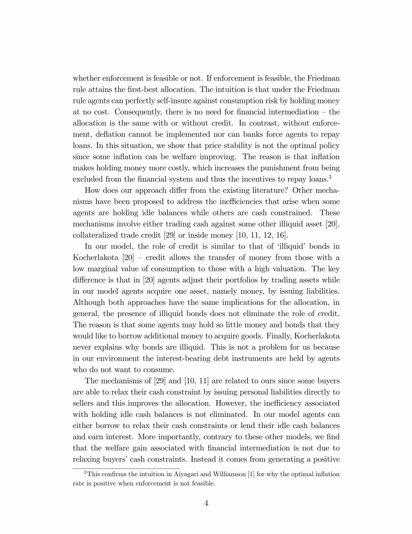
Figure 1. Cash and credit.

Although all goods transactions require money, buyers do not face a stan-dard cash-in-advance constraint. Before trading, they can borrow cash fromthe bank to supplement their money holdings but do so at the cost of thenominal interest rate as illustrated in Figure 1, which describes the flow ofgoods, credit and money in our model for markets 1 and 2. Note the absenceof links between the seller and the bank.11 The missing link is consistent withthe assumption that there is no record-keeping in the goods market due toanonymity. For example, it rules out the following mechanism. At the end ofeach period, every agent reports to the bank the identity of the trading part-ners and the quantities traded. If the report of an agent does not match thereport of his trading partner, then the bank punishes both agents by excludingthem from the banking system. This mechanism requires that the agents inthe good market can accurately identify their trading partners, which violatesour assumption of anonymity.12

Default. In any model of credit, default is a serious issue. We first assumethat banks can force repayment at no cost. In such an environment, defaultis not possible so agents face no borrowing constraints. In this case, banksare nothing more than cash machines that post interest rates for depositsand loans. In equilibrium these posted interest rates clear the market. We

11At the beginning of market 1 the seller deposits money at the bank which is redeemedin market 2. These two transactions, however, are independent from the flow of moneybetween buyer and bank and buyer and seller as described in Figure 1.

12It also excludes commonly used forms of payments such as credit card or check pay-ments. Such payments require that all agents must identify themselves and the value of theirgoods transactions to the banking system. With this information, money is not essentialsince all exchange can be done via record keeping.

8

then consider an environment where banks cannot force agents to repay. Theonly punishment available is that a borrower who fails to repay his loan isexcluded from the financial sector in all future periods. Given this punishment,we derive conditions to ensure voluntary repayment and show that this mayinvolve binding borrowing constraints, i.e. credit rationing.

Welfare. At the beginning of a period before types are realized, the expectedsteady state lifetime utility of the representative agent is

(1− β)W = (1− n)u (qb)− nc (qs) + U(x)− x (1)

where qb is consumption and qs production in market 2. We use (1) as ourwelfare criteria.To derive the welfare maximizing quantities we assume that all agents

are treated symmetrically. The planner then maximizes (1) subject to thefeasibility constraint

(1− n) qb = nqs. (2)

The first-best allocation satisfies

U 0 (x∗)= 1 and

u0 (q∗)= c0µ1− n

nq∗¶. (3)

where q∗ ≡ q∗b =n

(1−n)q∗s . These are the quantities chosen by a social planner

who could force agents to produce and consume.

3 Symmetric equilibrium

The timing in our model is as follows. At the beginning of the first marketagents observe their production and consumption shocks and they receive thelump-sum transfers τ 1M−1. Then, the banking sector opens and agents canborrow or deposit money. Finally, the banking sector closes and agents tradegoods. In the second market agents trade goods and settle financial claims.In period t, let φ be the real price of money in the second market. We

focus on symmetric and stationary equilibria where all agents follow identicalstrategies and where real allocations are constant over time. In a stationaryequilibrium end-of-period real money balances are time-invariant

φM = φ+1M+1. (4)

9

Moreover, we restrict our attention to equilibria where γ is time invariantwhich implies that φ/φ+1 = P+1/P =M+1/M = γ.13

Consider a stationary equilibrium. Let V (m) denote the expected valuefrom trading in market 1 with m money balances at time t. Let W (m, , d)

denote the expected value from entering the second market with m units ofmoney, loans, and d deposits at time t. In what follows, we look at arepresentative period t and work backwards from the second to the first market.

3.1 The second market

In the second market agents produce h goods and consume x, repay loans,redeem deposits and adjust their money balances. If an agent has borrowedunits of money, then he pays (1 + i) units of money, where i is the nominalloan rate. If he has deposited d units of money, he receives (1 + id) d, whereid is the nominal deposit rate. The representative agent’s program is

W (m, , d) = maxx,h,m+1

[U (x)− h+ βV+1 (m+1)] (5)

s.t. x+ φm+1 = h+ φ (m+ τ 2M−1) + φ (1 + id) d− φ (1 + i)

where m+1 is the money taken into period t + 1 and φ is the real price ofmoney. Rewriting the budget constraint in terms of h and substituting into(5) yields

W (m, , d) = φ [m+ τ 2M−1 − (1 + i) + (1 + id) d]

+maxx,m+1

[U (x)− x− φm+1 + βV+1 (m+1)] .

The first-order conditions are U 0 (x) = 1 and

φ = βV 0+1 (m+1) (6)

where V 0+1 (m+1) is the marginal value of an additional unit of money taken

into period t+ 1. Notice that the optimal choice of x is the same across timefor all agents and the m+1 is independent of m. As a result, the distributionof money holdings is degenerate at the beginning of the following period. Theenvelope conditions are

Wm=φ (7)

W =−φ (1 + i) (8)

Wd=φ (1 + id) . (9)

13This eliminates stationary equilibria where γ is stochastic.

10

3.2 The first market

Let qb and qs, respectively, denote the quantities consumed by a buyer andproduced by a seller trading in market 1. Let p be the nominal price of goodsin market 1. While we use competitive pricing for most of what we do, wealso consider matching and bargaining later on to compare the allocation withfinancial intermediation to the allocation in Lagos and Wright [21].It is straightforward to show that agents who are buyers will never deposit

funds in the bank and sellers will never take out loans. Thus, s = db = 0.

In what follows we let denote loans taken out by buyers and d depositsof sellers. We also drop these arguments in W (m, , d) where relevant fornotational simplicity.An agent who hasm money at the opening of the first market has expected

lifetime utility

V (m) = (1− n) [u (qb) +W (m+ τ bM−1 + − pqb, )]

+n [−c (qs) +W (m+ τ sM−1 − d+ pqs, d)](10)

where pqb is the amount of money spent as a buyer and pqs the money receivedas a seller. Once the preference shock occurs, agents become either a buyeror a seller. Note that sellers cannot deposit receipts of cash, pqs, earned fromselling in market 1. In short, the bank closes before the onset of trading inmarket 1.

Sellers’ decisions. If an agent is a seller in the first market, his problem is

maxqs,d

[−c (qs) +W (m+ τ sM−1 − d+ pqs, d)]

s.t. d ≤ m+ τ sM−1.

The first-order conditions are

−c0 (qs) + pWm=0

−Wm +Wd − λd=0.

where λd is the Lagrangian multiplier on the deposit constraint. Using (7),the first condition reduces to

c0 (qs) = pφ. (11)

Sellers produce such that the ratio of marginal costs across markets (c0 (qs) /1)is equal to the relative price (pφ) of goods across markets. Due to the linearity

11

of the envelope conditions, qs is independent of m and d. Consequently, sellersproduce the same amount no matter how much money they hold or whatfinancial decisions they make. Finally, it is straightforward to show that forany id > 0 the deposit constraint is binding and so sellers deposit all theirmoney balances.

Buyers’ decisions. If an agent is a buyer in the first market, his problemis

maxqb,

[u (qb) +W (m+ τ bM−1 + − pqb, )]

s.t. pqb ≤ m+ τ bM−1 +

≤ .̄

Notice that buyers cannot spend more cash than they bring into the firstmarket, m, plus their borrowing, , and the transfer τ bM−1. They also face theconstraint that the loan size is bounded above by .̄ They take this constraintas given. However, in equilibrium it is determined endogenously.Using (7), (8) and (11) the buyer’s first-order conditions reduce to

u0 (qb)= c0 (qs) (1 + λ/φ) (12)

φi=λ− λ (13)

where λ is the multiplier on the buyer’s cash constraint and λ on the borrowingconstraint. If λ = 0, then (12) reduces to u0 (qb) = c0 (qs) implying trades areefficient.For λ > 0, these first-order conditions yield

u0 (qb)

c0 (qs)= 1 + i+ λ /φ.

If λ = 0, thenu0 (qb)

c0 (qs)= 1 + i. (14)

In this case the buyer borrows up to the point where the marginal benefit ofborrowing equals the marginal cost. He spends all his money and consumesqb = (m+ τ bM−1 + ) /p. Note that for i > 0 trades are inefficient. In effect,a positive nominal interest rate acts as tax on consumption.Finally, if λ > 0

u0 (qb)

c0 (qs)> 1 + i. (15)

12

In this case the marginal value of an extra unit of a loan exceeds the mar-ginal cost. Hence, a borrower would be willing to pay more than the pre-vailing loan rate. However, if banks are worried about default, then theinterest rate may not rise to clear the market and credit rationing occurs.Consequently, the buyer borrows ,̄ spends all of his money and consumesqb =

¡m+ τ bM−1 +

¢̄/p.

Since all buyers enter the period with the same amount of money and facethe same problem, qb is the same for all of them. The same is true for thesellers. Finally, market clearing implies

qs =1− n

nqb. (16)

Banks. Banks accept nominal deposits, paying the nominal interest rate id,and make nominal loans at nominal rate i. The banking sector is perfectlycompetitive with free entry, so banks take these rates as given. There is nostrategic interaction among banks or between banks and agents. In particular,there is no bargaining over terms of the loan contract. Finally, we assume thatthere are no operating costs or reserve requirements.The representative bank solves the following problem per borrower

max (i− id)

s.t. ≤ ¯

u (qb)− (1 + i) φ ≥ Γ

where Γ is the reservation value of the borrower. The reservation value is theborrower’s surplus from receiving a loan at another bank. We investigate twoassumptions about repayment. In the first case, banks can force repaymentat no cost so the borrowing constraint is ¯ = ∞. In the second case, weassume that a borrower who fails to repay his loan will be shut out of thebanking sector in all future periods. Given this punishment, we need to deriveconditions to ensure voluntary repayment which determines .̄The first-order condition is

i− id − λL + λΓ

∙u0 (qb)

dqbd− (1 + i)φ

¸= 0

where λL and λΓ are the Lagrange multipliers on the lending constraint andparticipation constraint of the borrower respectively. For i− id > 0 the bank

13

would like to make the largest loan possible to the borrower. Thus, the bankwill always choose a loan size such that λΓ > 0.With free entry banks make zero profits so i = id. Since, dqb/d = φ/c0 (qs)

we haveu0 (qb)

c0 (qs)= 1 + i+

λLλΓφ

.

If λL = 0 the loan offered by the bank implies (14) so repayment is not anissue. If λL > 0 the constraint on the loan size is binding and implies (15).In a symmetric equilibrium all buyers borrow the same amount, , and sellersdeposit the same amount, d, so loan market clearing requires

(1− n) = nd. (17)

Marginal value of money. Using (10) the marginal value of money is

V 0 (m) = (1− n)u0 (qb)

p+ nφ (1 + id) .

In the appendix we show that the value function is concave inm so the solutionto (6) is well defined.Using (11) V 0 (m) reduces to

V 0 (m) = φ

∙(1− n)

u0 (qb)

c0 (qs)+ n (1 + id)

¸. (18)

The marginal value of money has two components. If the agent is a buyer hereceives u0 (qb) /c0 (qs) from spending the marginal unit of money. This effectis standard. Now, if he is a seller he can lend the unit of money and receive1 + id. Thus, financial intermediation increases the marginal value of moneybecause sellers can deposit idle cash and earn interest.

4 Equilibrium with enforcement

In this section, as a benchmark, we assume that the monetary authority canimpose lump-sum taxes and banks can force repayment of loans at no cost.This does not imply that the banks or the monetary authority can dictate theterms of trade between private agents in the goods market.In any stationary monetary equilibrium use (6) lagged one period to elim-

inate V 0 (m) from (18). Then use (4) and (16) to get

γ − β

β= (1− n)

"u0 (qb)

c0¡1−nnqb¢ − 1#+ nid. (19)

14

The right-hand side measures the value of bringing one extra unit of moneyinto the first market. The first term reflects the net benefit (marginal utilityminus marginal cost) of spending the unit of money on goods when a buyerand the second term is the value of depositing an extra unit of idle balanceswhen a seller.Since banks can force agents to repay their loans, agents are unconstrained

so ¯=∞. This implies that (14) holds. Using it in (19) yields14

γ − β

β= (1− n) i+ nid. (20)

Now, the first term on the right-hand side reflects the interest saving fromborrowing one less unit of money when a buyer.Zero profit implies i = id and so

γ − β

β= i. (21)

We can rewrite this in terms of qb using (14) to get

γ − β

β=

u0 (qb)

c0¡1−nnqb¢ − 1. (22)

Definition 1 When repayment of loans can be enforced, a monetary equilib-rium with credit is an interest rate i satisfying (21) and a quantity qb satisfying(22).

Proposition 1 Assume repayment of loans can be enforced. Then if γ > β,a unique monetary equilibrium with credit exists. Equilibrium consumption isdecreasing in γ, and satisfies qb < q∗ with qb → q∗ as γ → β.

It is clear from (22) that money is neutral, but not super-neutral. In-creasing its stock has no effect on qb, while changing the growth rate γ does.Moreover, the Friedman rule (γ = β) generates the first-best allocation.How does this allocation differ from the allocation in an economy without

credit? Let q̃b denote the quantity consumed when there is no financial in-termediation. It is straightforward to show that q̃b solves (19) with id = 0,i.e.,

γ − β

β= (1− n)

"u0 (q̃b)

c0¡1−nnq̃b¢ − 1# . (23)

14This equation implies that if nominal bonds could be traded in market 2, their nominalrate of return, ib, would be (1− n) i+nid. Thus agents would be indifferent between holdinga nominal bond or holding a bank deposit.

15

Comparing (23) to (22), it is clear that q̃b < qb for any γ > β. Thus, we haveproved the following

Corollary 1 For γ > β financial intermediation improves the allocation andwelfare.

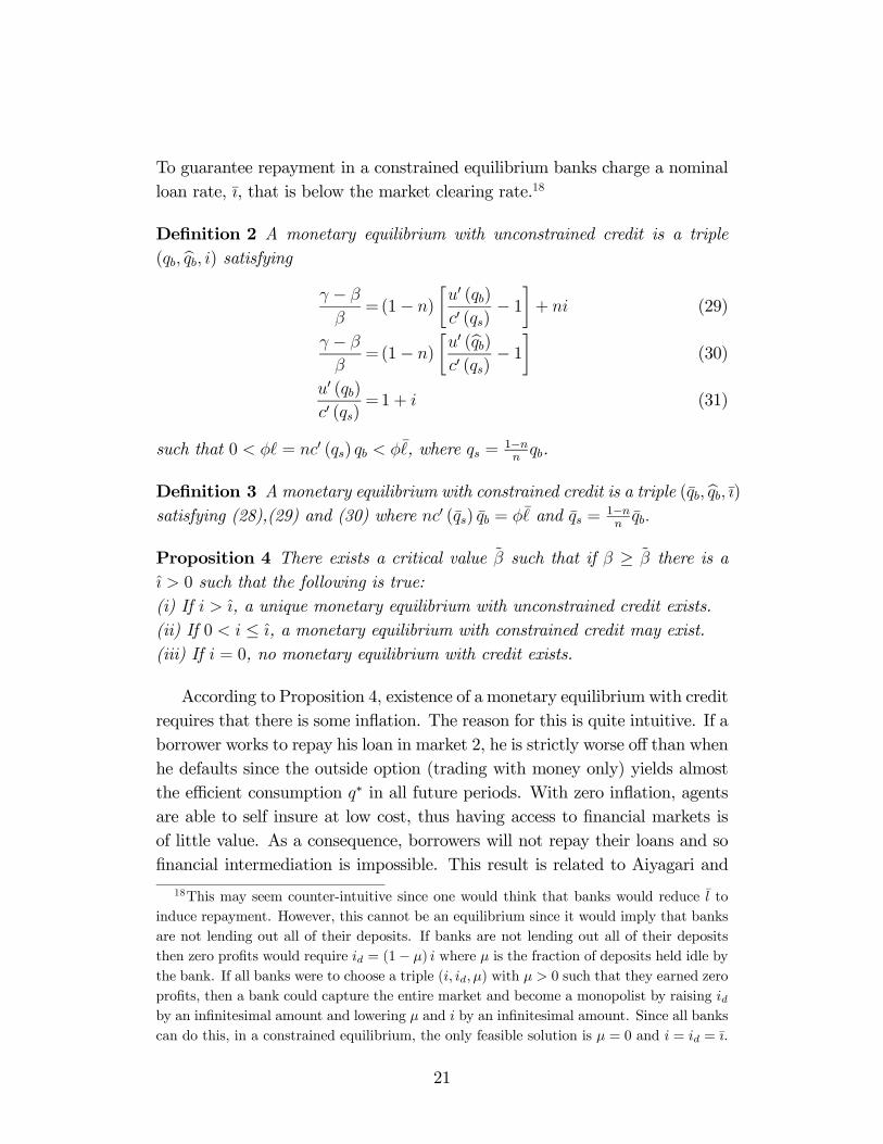
The key result of this section is that financial intermediation improves theallocation away from the Friedman rule. The greatest impact on welfare is formoderate values of inflation. The reason is that near the Friedman rule there islittle gain from redistributing idle cash balances while for high inflation ratesmoney is of little value anyway. At the Friedman rule agents can perfectlyself-insure against consumption risk because the cost of holding money is zero.Consequently, there is no welfare gain from financial intermediation.15

1 1.5 2 2.5 3γ

0.2

0.4

0.6

0.8

1

1.2

1.4

DW

β

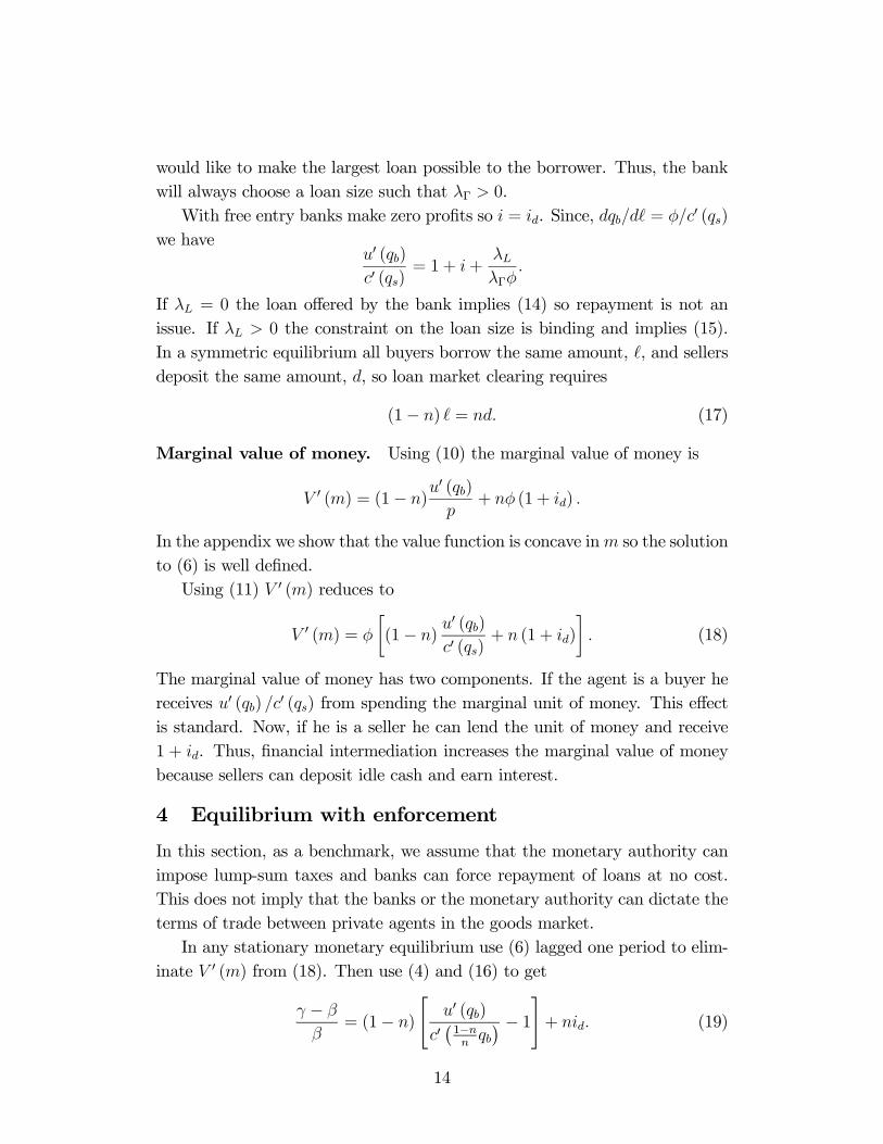
Figure 2: Difference in welfare.

The welfare implications of financial intermediation are displayed in Figure2. The graph shows the difference (DW =W b−W nb) in the expected lifetimeutilities with financial intermediation (W b) and without (W nb) as a function ofthe inflation rate γ. Note that the difference is equal to zero when γ = β (at theorigin), converges to zero when γ →∞ and is maximal for some intermediaterate of inflation. Figure 2 is drawn with the utility function u (q) = q0.8/0.8,cost function c (q) = q, discount factor β = 0.95 and measure of sellers n = 0.4.

15With extensive margin externalities as in [4] or [30], being away from the Friedmanrule can be optimal. In this case, financial intermediation clearly is welfare improving.

16

Given that financial intermediation improves the allocation away from theFriedman rule, is it because it relaxes borrowers’ liquidity constraints or be-cause it allows payment of interest to depositors? The following propositionanswers this question.

Proposition 2 The gain in welfare from financial intermediation is due tothe fact that it allows payment of interest to depositors and not from relaxingborrowers’ liquidity constraints.

According to Proposition 2 the gain in welfare comes from payment of in-terest to agents holding idle balances. To prove this claim we show in the proofof Proposition 2 that in equilibrium, agents are indifferent between borrowingto finance equilibrium consumption or bringing in a sufficient amount of cashto finance the same consumption. The only importance of borrowing is to sus-tain payment of interest to depositors. That is, even though each individualagent is indifferent between borrowing and not borrowing, agents taking outloans are needed to finance the interest received by the depositors.As a final proof of this argument, we consider a systematic government pol-

icy that redistributes cash in market 1 by imposing lump-sum taxes on sellersand giving the cash as lump-sum transfers to buyers. This clearly relaxes theliquidity constraints of the buyers while paying no interest to depositors. How-ever, inspection of (23) reveals that neither τ 1 nor τ b appear in this equation.Hence, varying the transfer across the two markets or by redistributing cashfrom sellers to buyers in a predictable, lump-sum fashion has no effect on q̃b. Itonly affects the equilibrium price of money in the last market. Agents simplychange the amount of money they bring into market 1 and so the demand formoney changes in market 2, which alters the price of money φ. Note also thatthis implies that the allocation with credit cannot be replicated by governmentpolicies using lump-sum transfers or taxes.Finally, we would like to see how the equilibrium allocation in our credit

model compares with Lagos and Wright [21]. Towards this end, we now con-sider matching and bargaining in market 1 as an alternative to Walrasianpricing.

Bargaining For simplicity we assume n = 1/2 and τ b = τ s = τ . The timingis similar as before in that agents observe their preference shocks, then go tothe bank to borrow and deposit funds. The bank then closes. The difference isthat buyers now are paired with sellers and they bargain according to the gen-

17

eralized Nash protocol over the quantity of goods and money to be exchanged.The decisions in market 2 are unaffected.The value function for each agent at the opening of market 1 is

V (m) = 12[u (qb) +W (m+ τM−1 + − zb, )]

+12[−c (qs) +W (m+ τM−1 − d+ zs, d)]

where zb is the amount of money given up when a buyer and zs is the amountreceived when a seller.Due to the linearity of W (m, , d), the bargaining problem is

maxq,z

[u (q)− φz]θ [−c (q) + φz]1−θ

s.t. z ≤ m+ τM−1 +

where θ is the buyer’s bargaining weight. As in Lagos and Wright [21], thesolution to the bargaining problem yields

φz = g (q) ≡ θc(q)u0(q) + (1− θ)u(q)c0(q)

θu0(q) + (1− θ)c0(q)

where g0 (q) > 0. If θ < 1, then g0 (q) > c0 (q) while for θ = 1, g0 (q) = c0 (q) .

In any monetary equilibrium, the buyer will spend all of his cash holdings soz = m+ τM−1+ . It then follows that dz/dm = 1 and ∂q/∂m = φ/g0 (q) > 0.To determine borrowing and lending choices, we still have that sellers will

deposit all of their money in the bank. Those who are buyers now maximize

maxu (q) +W (m+ τM−1 + − z, )

s.t. z ≤ m+ τM−1 + .

It is straightforward to show that the solution yields

u0 (q)

g0 (q)= 1 + i. (24)

Differentiating V (m) and rearranging gives

V 0 (m) =φ

2

∙u0 (q)

g0 (q)+ 1 + id

¸.

Using (6) lagged one period, (24) and i = id yields

γ − β

β=

u0 (q)

g0 (q)− 1 = i. (25)

18

The interesting aspect of this result is that the nominal interest rate withbargaining is exactly the same as it is with competitive pricing. It then followsfrom (24) that the quantity traded in all matches under bargaining is lowerthan under competitive pricing since g0 (q) > c0 (q). This is due to the holdupproblem that occurs on money demand under bargaining.How does the allocation here compare to the allocation in Lagos andWright

[21]? Their equilibrium value of q solves16

γ − β

β=1

2

∙u0 (q)

g0 (q)− 1¸. (26)

It is clear that the quantity solving (25) is greater than the quantity solving(26). Thus the existence of a credit market increases output and welfare evenwith bargaining.17

5 Equilibrium without enforcement

In the previous section enforcement occurred in two occasions. First, themonetary authority could impose lump-sum taxes. Second, banks could forcerepayment of loans. Here, we assume away any enforcement. The first impli-cation is that the monetary authority cannot run a deflation. Consequently,γ ≥ 1. The second is that those who borrow in market 1 have an incentive todefault in market 2. To offset this short-run benefit we assume that if an agentdefaults on his loan then the only punishment is permanent exclusion from thebanking system. This is consistent with the requirement that all trades arevoluntary since banks can refuse to trade with private agents. Furthermore,it is in the banks’ best interest to share information about agents’ repaymenthistories.For credit to exist, it must be the case that borrowers prefer repaying loans

to being banished from the banking system. Given this punishment, the realborrowing constraint φ¯ is endogenous and we need to derive conditions toensure voluntary repayment. In what follows, since the transfers only affectprices, we set τ b = τ s = τ 1 > 0.For buyers entering the second market with no money and who repay their

loans, the expected discounted utility in a stationary equilibrium is

W (m) = U (x∗)− hb + βV+1 (m+1)

16This is the expression if one sets σ = 1/2 in their model.17A similar result is found in [14] using a model of competitive search where market

makers can charge differential entry fees for buyers and sellers.

19

where hb is a buyer’s production in the second market if he repays his loan.Consider the case of a buyer who defaults on his loan. The benefit of

defaulting is that he has more leisure in the second market because he doesnot work to repay the loan. The cost is that he is out of the banking system,meaning that he cannot borrow or deposit funds for the rest of his life. Hecannot lend because the bank would confiscate his deposits to settle his loanarrears. Thus, a deviating buyer’s expected discounted utility is

cW (m) = U (bx)− bhb + βbV+1 (m̂+1)

where the hat indicates the optimal choice by a deviator. The value of beingin the banking system W (m) as well as the expected discounted utility ofdefection cW (m) depend on the growth rate of the money supply γ. This putsconstraints on γ that the monetary authority can impose without destroyingfinancial intermediation.Existence of a monetary equilibrium with credit requires that W (m) ≥cW (m), where the real borrowing constraint φ¯ satisfies

W (m) = cW (m) . (27)

Given a borrowing constraint there are two possibilities: 1) the borrowingconstraint is nonbinding for all agents or 2) it binds for some agents. In anunconstrained equilibrium with credit we have φ < φ¯ and in a constrainedequilibrium φ = φ .̄ The following Lemma is used for the remainder of thissection.

Lemma 3 The real borrowing constraint φ¯ satisfies

φ¯=β

(1 + i) (1− β)

½(1− n)Ψ (qb, bqb) + c0 (qs)

µγ − β

β

¶[bqb − (1− n) qb]

¾(28)

whereΨ (qb, bqb) = u (qb)− u (bqb)− c0 (qs) (qb − bqb) ≥ 0.

In any equilibrium, banks lend out all of their deposits so real lendingsatisfies

φ =n

1− nφM.

20

To guarantee repayment in a constrained equilibrium banks charge a nominalloan rate, ı̄, that is below the market clearing rate.18

Definition 2 A monetary equilibrium with unconstrained credit is a triple(qb, bqb, i) satisfying

γ − β

β=(1− n)

∙u0 (qb)

c0 (qs)− 1¸+ ni (29)

γ − β

β=(1− n)

∙u0 (bqb)c0 (qs)

− 1¸

(30)

u0 (qb)

c0 (qs)=1 + i (31)

such that 0 < φ = nc0 (qs) qb < φ ,̄ where qs = 1−nnqb.

Definition 3 Amonetary equilibrium with constrained credit is a triple (q̄b, bqb, ı̄)satisfying (28),(29) and (30) where nc0 (q̄s) q̄b = φ¯ and q̄s = 1−n

nq̄b.

Proposition 4 There exists a critical value β̃ such that if β ≥ β̃ there is aı̂ > 0 such that the following is true:(i) If i > ı̂, a unique monetary equilibrium with unconstrained credit exists.(ii) If 0 < i ≤ ı̂, a monetary equilibrium with constrained credit may exist.(iii) If i = 0, no monetary equilibrium with credit exists.

According to Proposition 4, existence of a monetary equilibrium with creditrequires that there is some inflation. The reason for this is quite intuitive. If aborrower works to repay his loan in market 2, he is strictly worse off than whenhe defaults since the outside option (trading with money only) yields almostthe efficient consumption q∗ in all future periods. With zero inflation, agentsare able to self insure at low cost, thus having access to financial markets isof little value. As a consequence, borrowers will not repay their loans and sofinancial intermediation is impossible. This result is related to Aiyagari and

18This may seem counter-intuitive since one would think that banks would reduce l̄ toinduce repayment. However, this cannot be an equilibrium since it would imply that banksare not lending out all of their deposits. If banks are not lending out all of their depositsthen zero profits would require id = (1− µ) i where µ is the fraction of deposits held idle bythe bank. If all banks were to choose a triple (i, id, µ) with µ > 0 such that they earned zeroprofits, then a bank could capture the entire market and become a monopolist by raising idby an infinitesimal amount and lowering µ and i by an infinitesimal amount. Since all bankscan do this, in a constrained equilibrium, the only feasible solution is µ = 0 and i = id = ı̄.

21

Williamson [1] who also report a break-down of financial intermediation closeto the Friedman rule in a dynamic contracting model with private information.For low rates of inflation credit rationing occurs. Again, in this case the cost

of using money to self insure is low. To induce repayment banks charge a belowmarket-clearing interest rate since this reduces the amount borrowers have torepay. In short, with an endogenous borrowing constraint, the interest rate islower than would occur in an economy where banks can force repayment.19

One aspect that is puzzling about this result is that the incentive to de-fault is higher for low nominal interest rates and lower for high nominal in-terest rates. This seems counter-intuitive at first glance since standard credit-rationing models, such as [31], suggest that the likelihood of default increasesas interest rates rise. The reason for the difference is that standard credit ra-tioning models focus on real interest rates, while our model is concerned withnominal interest rates. In our model, nominal rates rise because of perfectlyanticipated inflation, which acts as a tax on a deviator’s wealth since he carriesmore money for transactions purposes. This reduces the incentive to defaultthereby alleviating the need to ration credit. Consequently, a key contribu-tion of our analysis is to show how credit rationing can arise from changes innominal interest rates.

Is Inflation Welfare Improving? In an unconstrained borrowing equilib-rium, it is straightforward to show that inflation is always welfare reducingsince it reduces the real value of money balances and consumption for allagents. However, in a constrained borrowing equilibrium, it may be optimalfor the monetary authority to set γ > 1 since inflation increases the cost ofbeing excluded from the banking system. This relaxes the borrowing con-straint and creates a first-order welfare gain. We would like to know underwhat conditions the optimal inflation rate is positive. We can thus state thefollowing

Proposition 5 In a constrained credit equilibrium, if β > (1 + n)−1, then apositive steady state inflation rate maximizes welfare.

Thus, as long as agents are sufficiently patient, inflation is welfare improv-ing. By relaxing the budget constraint, inflation allows the nominal interestrate to increase towards the market clearing level. This increases the compen-sation sellers receive for bringing in idle money balances yet it does not crowd

19Similar results occur in [18], [17] or [2].

22

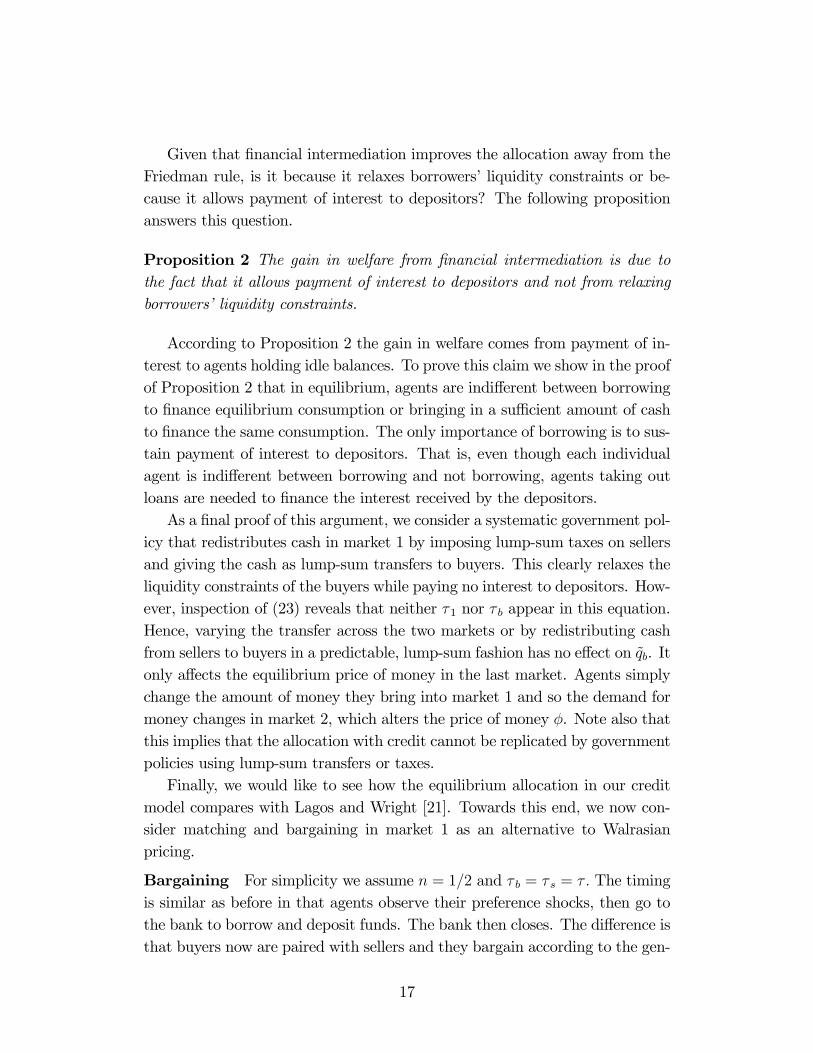
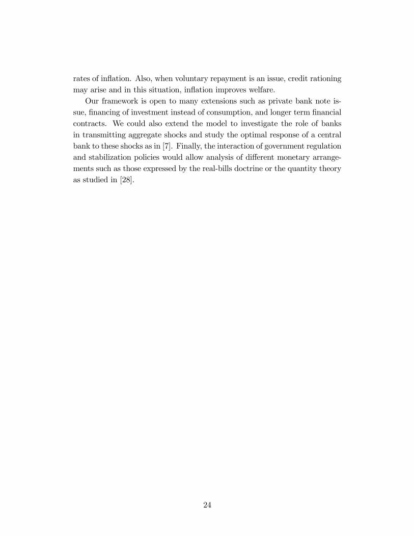
out consumption by buyers since they are credit constrained. Consequently,the demand for money in market 2 increases, which raises the real value ofmoney and qb. To illustrate this proposition we solve the model numericallyand the results are contained in Figure 3.

1.005 1.01 1.015 1.02γ

2.15

2.25

2.3

2.35

2.4

2.45

W

á welfare without credit

constrained credit unconstrained credit

γ

Figure 3: Welfare with endogenous borrowing constraint.

Figure 3 is a numerical example of our economy in which the equilibriumwith credit exists and is unique. The solid line is the equilibrium with creditwhile the dashed line is the equilibrium without credit. At the origin, γ =1, the constrained credit equilibrium breaks down so the allocation is thesame as the equilibrium without credit. When γ < eγ, where eγ = β (1 + ı̂),the borrowing constraint is binding and welfare is increasing in γ and whenγ > eγ the borrowing constraint is not binding and welfare is decreasing in γ.Note that the equilibrium with credit has higher welfare than the equilibriumwithout credit even if there is rationing.

6 Conclusion

In this paper we have shown how money and credit can coexist in a modelwhere money is essential. Our main findings are that reallocating idle cash viafinancial intermediation can expand output and improve welfare away from theFriedman rule but not at the Friedman rule. Furthermore, such an improve-ment cannot be achieved through a government policy of lump-sum taxes andtransfers. Interestingly, financial intermediation is most valuable for moderate

23

rates of inflation. Also, when voluntary repayment is an issue, credit rationingmay arise and in this situation, inflation improves welfare.Our framework is open to many extensions such as private bank note is-

sue, financing of investment instead of consumption, and longer term financialcontracts. We could also extend the model to investigate the role of banksin transmitting aggregate shocks and study the optimal response of a centralbank to these shocks as in [7]. Finally, the interaction of government regulationand stabilization policies would allow analysis of different monetary arrange-ments such as those expressed by the real-bills doctrine or the quantity theoryas studied in [28].

24

References

[1] S. Aiyagari, S. Williamson, Money and dynamic credit arrangements withprivate information, J. of Econ. Theory 91 (2000), 248-279.

[2] F. Alvarez, U. Jermann, Efficiency, equilibrium and asset pricing withrisk of default, Econometrica 68 (2000), 775-797.

[3] S. B. Aruoba, C. Waller, R. Wright, Money and capital, Working paper,University of Pennsylvania, 2006.

[4] A. Berentsen, G. Rocheteau, S. Shi, “Friedman meets Hosios: efficiencyin search models of money,” Economic Journal, forthcoming.

[5] A. Berentsen, G. Camera, C. Waller, The distribution of money and pricesin an equilibrium with lotteries, Econ. Theory 24 (2004), 887-906.

[6] A. Berentsen, G. Camera, C. Waller, The distribution of money balancesand the non-neutrality of money, Int. Econ. Rev. 46 (2005), 465-487.

[7] A. Berentsen, C. Waller, Optimal stabilization policy with flexible prices,CESifo Working Paper No. 1638 (2005).

[8] T. Bewley, The optimum quantity of money, in John H. Kareken andNeil Wallace, eds., Models of Monetary Economies, Minneapolis: FederalReserve Bank of Minneapolis, 1980, pp. 169-210.

[9] G. Camera, D. Corbae, Money and price dispersion, Int. Econ. Rev. 40(1999), 985-1008.

[10] R. Cavalcanti, N. Wallace, Inside and outside money as alternative mediaof exchange, J. of Money, Credit, and Banking 31 (Part 2) (1999a), 443-457.

[11] R. Cavalcanti, N. Wallace, A model of private bank-note issue, Rev. Econ.Dynam. 2 (1999b), 104-136.

[12] R. Cavalcanti, A. Erosa, T. Temzelides, Private money and reserve man-agement in a random-matching model, J. of Polit. Economy 107 (1999),929-945.

[13] M. Faig, Money and banking in an economy with villages, Working paper,University of Toronto, 2004.

[14] M. Faig, X. Huangfu, Competitive search equilibrium in monetaryeconomies, J. of Econ. Theory (forthcoming)

[15] E. Green, R. Zhou, Money as a mechanism in a Bewley economy, Int.Econ. Rev. 46 (2005), 351-371.

[16] P. He, L. Huang, R. Wright, Money and banking in search equilibrium,Int. Econ. Rev. 46 (2005), 631-670.

25

[17] C. Hellwig, G. Lorenzoni, Bubbles and private liquidity, Working paper,UCLA, 2004.

[18] T. Kehoe, D. Levine, Debt-constrained asset markets, Rev. Econ. Stud.60 (1993), 865-888.

[19] N. Kocherlakota, Money is memory, J. of Econ. Theory 81 (1998), 232—251.

[20] N. Kocherlakota, Societal benefits of illiquid bonds, J. of Econ. Theory108 (2003), 179-193.

[21] R. Lagos, R. Wright, A unified framework for monetary theory and policyanalysis, J. of Polit. Economy 113 (2005), 463-484.

[22] R. Lagos, G. Rocheteau, Inflation, output and welfare, Int. Econ. Rev. 46(2005), 495-522.

[23] D. Levine, Asset trading mechanisms and expansionary policy, J. of Econ.Theory 54 (1991), 148-164.

[24] R. E. Lucas, Equilibrium in a pure currency economy, in John H. Karakenand Neil Wallace, eds., Models of Monetary Economics, Minneapolis: Fed-eral Reserve Bank of Minneapolis, 1980, pp. 131-145

[25] R. E. Lucas, N. Stokey, Optimal fiscal and monetary policy in an economywithout capital, J. of Monet. Econ. 12 (1983), 55-93.

[26] M. Molico, The distribution of money and prices in search equilibrium.Int. Econ. Rev. (forthcoming)

[27] G. Rocheteau, R. Wright, Money in search equilibrium, in competi-tive equilibrium and in competitive search equilibrium, Econometrica 73(2004), 175-202.

[28] T. Sargent, N. Wallace, The real-bills doctrine versus the quantity theory:a reconsideration, J. of Polit. Economy 90 (6) (1982), 1212-1236.

[29] S. Shi, Credit and money in a search model with divisible commodities,Rev. of Econ. Stud. 63 (1996), 627-652.

[30] S. Shi, A divisible search model of fiat money, Econometrica 65 (1997),75-102.

[31] J. Stiglitz, A. Weiss, Credit rationing in markets with imperfect informa-tion, Am. Econ. Rev. 71 (1981), 393-410.

[32] N. Wallace, Narrow banking meets the Diamond-Dybvig model, FederalReserve Bank of Minneapolis Quarterly Review 20 (1) (1996), Winter,3-13.

[33] N. Wallace, Whither monetary economics?, Int. Econ. Rev. 42 (2001),847-869.

26

Appendix

Proof that V (m) is concave ∀m. Differentiating (10) with respect to m

V 0 (m) = (1− n)£u0 (qb)

∂qb∂m+Wm

¡1− p∂qb

∂m+ ∂

∂m

¢+W ∂

∂m

¤+n£−c0 (qs) ∂qs∂m

+Wm

¡1 + p∂qs

∂m− ∂d

∂m

¢+Wd

∂d∂m

¤Recall from (7), (8), and (9) that Wm = φ, W = −φ (1 + i) and Wd =

φ (1 + id) ∀m. Furthermore, ∂qs/∂m = 0 because the quantity a seller pro-duces is independent of his money holdings. We also know that ∂d/∂m = 1

since a seller deposits all his cash when i > 0. Hence,

V 0 (m) = (1− n)£u0 (qb)

∂qb∂m+ φ

¡1− p∂qb

∂m+ ∂

∂m

¢− φ (1 + i) ∂

∂m

¤+nφ (1 + id)

Since i > 0 implies pqb = m+ τ bM−1+ we have 1−p (∂qb/∂m)+∂ /∂m = 0.Hence20

V 0 (m) = (1− n)u0 (qb) /p+ nφ (1 + id)

In a symmetric equilibrium qs =1−nnqb. Define m∗ = pq∗. Then if m < m∗,

0 < qb < q∗, implying ∂qb/∂m > 0 so that V 00 (m) < 0. If m ≥ m∗, qb = q∗

implying ∂qb/∂m = 0, so that V 00 (m) = 0. Thus, V (m) is concave ∀m.Proof of Proposition 1. Because u(q) is strictly concave there is a uniquevalue q that solves (14), and for γ > β, q < q∗ where q∗ is the efficient quantitysolving u0(q∗) = c0

¡1−nnq∗¢. As γ → β, u0 (q) → c0

¡1−nnq¢, q → q∗, and from

(21) i → 0. In this equilibrium, the Friedman rule sustains efficient tradesin the first market. Since V (m) is concave, then for γ > β, the choice m ismaximal.We now derive equilibrium consumption and production in the second mar-

ket. Recall that, due to idiosyncratic trade shocks and financial transactions,money holdings are heterogeneous after the first market closes. Therefore, ifwe set m = M−1, the money holdings of agents at the opening of the secondmarket are 0 for buyers and 1

n(1 + τ 1)M−1 for sellers.

Equation (6) gives us x∗ = U 0−1 (1). The buyer’s production in the secondmarket can be derived as follows

hb = x∗ + φ {m+1 + (1 + i) − τ 2M−1} = x∗ + c0 (qs) qb + inc0 (qs) qb

20Note that u0 (qb)∂qb∂m − φ (1 + i) ∂l

∂m = u0 (qb)∂qb∂m − φ (1 + i)

hp∂qb∂m − 1

i= ∂qb

∂m (u0 (qb)− φ (1 + i) p) + φ (1 + i) = φ (1 + i) = u0(qb)

p .

27

since in equilibrium

m+1=M =M−1 + τ1M−1 + τ 2M−1

c0 (qs) qb=φ [(1 + τ 1)M−1 + ]

φ =nc0 (qs) qb.

Thus, an agent who was a buyer in market 1 has to work to recover theproduction cost of his consumption and the interest on his loan. The seller’sproduction is

hs=x∗ + φ {m+1 − [pqs + (1 + τ 1)M−1 + idd+ τ 2M−1]}=x∗ − c0 (qs) qs − φidd

The expected hours worked h satisfies

h = (1− n)hb + nhs = x∗ (32)

since in equilibrium qb =n1−nqs and i (1− n) = idnd. Finally, hours in market

2 can be also expressed in terms of q as in the following tableTrading history: Production in the last market:Buy hb = x∗ + c0 (qs) (1− n) qb + ne (qb)u (qb)

Sell hs = x∗ − (1−n)n[c0 (qs) (1− n) qb + ne (qb)u (qb)]

Since we assumed that the elasticity of utility e (qb) is bounded, we canscale U(x) such that there is a value x∗ = U 0−1 (1) greater than the last termfor all qb ∈ [0, q∗]. Hence, hs is positive for for all qb ∈ [0, q∗] ensuring that theequilibrium exists.Proof of Proposition 2. Assume that at some point in time t an agentat the beginning of market 2 chooses never to borrow again but continues todeposit. The first thing to note is that it is optimal for him to buy the samequantity qb since his optimal choice still satisfies (22). This implies that hismoney balances are m̄+1 = m+1+ +1. An agent who decides to never borrowhas to carry more money but he saves the interest on loans in the future. Inparticular, consumption and production in the market 1 are not affected. Thedifference in lifetime payoffs come from difference in hours worked.If he enters market 2 having been a buyer, the hours worked are

h̄b=x∗ + φ {m+1 + +1 + (1 + i) − τ 2M−1}=x∗ + c0 (qs) qb + φ +1 + φi

28

while if he sold in market 1 he works

h̄s=x∗ + φ {m+1 + +1 − [pqs + (1 + i) d+ τ 2M−1]}=x∗ − c0 (qs) qs + φ +1 − φidd

The expected hours worked satisfy

h̄ = (1− n) h̄b + nh̄s = x∗ + φ +1

Consequently, from (32) the additional hours worked are

h̄− h = φ +1 = γnc0 (qs) qb > 0 (33)

since +1 = γ in a steady state.Let us next consider the hours worked in market 2 in some future period.

Since he has no loan to repay the hours worked are

h̆b=x∗ + φ {m+1 + +1 − τ 2M−1}=x∗ + c0 (qs) qb + nc0 (qs) qb (γ − 1)

if he was a buyer while if he sold in market 1 he works

h̆s=x∗ + φ©m+1 + +1 −

£pqs + (1 + i) d̄+ τ 2M−1

¤ª=x∗ + nc0 (qs) qb (γ − 1)− c0 (qs) qs − (γ − β) c0 (qs) qb/β

The expected hours worked h satisfies

h̆ = (1− n) h̆b + nh̆s = x∗ − nc0 (qs) qbγ (1− β) /β

The expected gain from this strategy in any future period is

h̆− h = −nc0 (qs) qbγ (1− β) /β < 0 (34)

Then, from (33) and (34), the total expected gain from this deviation is

h̄− h+β³h̆− h

´1− β

= 0.

So agents are indifferent to borrowing at the current rate of interest or takingin the equivalent amount of money themselves.Proof of Corollary 1.

29

Neither τ 1 nor τ b appear in (22). Therefore, (τ 1, τ 2) can only affect theequilibrium φ. Of course, by changing τ 1 we change τ 2, for a given rate ofgrowth of money. To see how the transfers affect φ note that φ = c0(qs)nqb.Since = n

1−nM−1(1 + τ s) =n1−nM(

1+τs1+τ

) and qs =1−nnqb then we have

φ =c0(qs)nqb

=(1− n)c0(1−n

nqb) (1 + τ)

M(1 + τ s)

which implies the price of money in the second market, φ, is affected by thetiming and size of lump-sum transfers.Proof of Lemma 3. Since the transfers do not affect quantities set τ b = τ s =

τ 1 = 0 and τ 2 = τ . We now derive the endogenous real borrowing constraintφ .̄ This quantity is the maximal real loan that a borrower is willing to repayin the second market at given market prices. For buyers entering the secondmarket with no money, who repay their loans, the expected discounted utilityin a steady state is

W (m) = U (x∗)− hb + βV+1 (m+1)

where hb is a buyer’s production in the second market if he repays his loan.Consider a borrower who borrowed .̄ in market 1 and is considering defaultingon his loans in market 2. A deviating buyer’s expected discounted utility is

cW (m) = U (bx)− bhb + βbV+1 (bm+1)

where the hat indicates the optimal choice by a deviator. Thus φ¯ is the valueof borrowing such that W (m) =cW (m) or

U (x∗)− U (bx) + bhb − hb + βhV+1 (m+1)− bV+1 (bm+1)

i= 0. (35)

The continuation payoffs are

bV+1 (bm+1)= (1− β)−1h(1− n)u (bqb)− nc (bqs) + U (x∗)− bhi

V+1 (m+1)= (1− β)−1 [(1− n)u (qb)− nc (qs) + U (x̂)− h] . (36)

We now derive bx, bqb, bqs and bhb. In the last market the deviating buyer’sprogram is

cW (bm)= maxx,hb,m̂+1

hU (bx)− bhb + βbV+1 (bm+1)

is.t. bx+ φbm+1 = bhb + φ (bm+ τ 2M−1) .

30

The first-order conditions are U 0 (bx) = 1 and −φ + βbV 0+1 (m̂+1) = 0. Thus,bx = x∗. In market one, it is straightforward to show that if the deviator is

a seller in the first market he sells −c0 (bqs) + pφ = 0. Hence, the deviatorproduces the same amount as non-deviating sellers so bqs = qs =

1−nnqb.

Finally, the marginal value of the money satisfies

bV 0+1 (m̂) = φ

∙(1− n) u0 (bqb)

c0 (qs)+ n

¸which means that the deviator’s choice of money balances satisfies

γ − β

β= (1− n)

∙u0 (bqb)c0 (qs)

− 1¸. (37)

Now if we compare (37) with (22) we find that for γ > β

1− n =u0 (qb)− c0 (qs)

u0 (bqb)− c0 (qs)(38)

implying bqb < qb. Thus, using (35) and (36) we obtain

hb − bhb = β

1− β

h(1− n) [u (qb)− u (bqb)] + bh− h

i. (39)

Deriving bhb − hb. If the buyer repays his loans he works

hb=x∗ + φm+1 − φ£m− ¯− pqb

¤− φτM−1 + φ (1 + i) ¯

=x∗ + i¯+ φpqb

where we use the equilibrium conditionm+1 = m+τM−1 = γm. If he defaultson his loans, he works

bhb=x∗ + φbm+1 − φ¡m− ¯− pqb

¢− φτM−1

=x∗ + φ (bm+1 −m+1)− φ¯+ φpqb

=x∗ + φγ (bm−m)− φ¯+ φpqb

where we use the equilibrium condition that a defaulter’s money balances mustgrow at the rate γ so bm+1 = bm+ τM−1 = γ bm. Note that how much he spentin the previous market 1 is the same whether he repays or not. Thus

hb − bhb=x∗ + φi¯+ φpqb − x∗ − φ (bm+1 −m+1) + φ¯− φpqε

=φ (1 + i) ¯− φγ (bm−m) . (40)

31

Deriving bh− h: Once the agent defaults, as a buyer he spends pbqb unitsof money so his hours worked are

bh=x∗ + φbm+1 − φ (bm− pbqb)− φτM−1

=x∗ + φ (bm+1 − bm) + φpbqb − φ (m+1 −m)

=x∗ + (γ − 1)φ (bm−m) + φpbqb.For a seller we have

bhs=x∗ + φbm+1 − φ (bm+ pbqs)− φτM−1

=x∗ + (γ − 1)φ (bm−m)− φp

µ1− n

n

¶qb.

So for a defaulter expected hours worked are bh = (1− n)bhb + nbhs = x∗ +

(γ − 1)φ (bm−m) while if he does not deviate he works h = x∗ and so

bh− h = (γ − 1)φ (bm−m) . (41)

Substituting (40) and (41) into (39) and rearranging yields

φ¯=β

(1 + i) (1− β)

½(1− n)Ψ (qb, bqb) + c0 (qs)

γ − β

β[bqb − (1− n) qb]

¾(42)

where Ψ (qb, bqb) = u (qb)− u (bqb)− c0¡1−nnqb¢(qb − bqb) > 0 since

u (qb)− u (bqb)qb − bqb > u0 (qb) > c0 (qs) (43)

for all γ > β. The RHS of (42) must be positive to have a credit equilibrium.For this to be positive, substitute (37) and (43) into (42) and rearrange toobtain

u (qb)− u (bqb)qb − bqb > u0 (qb)

qb − bqb u0(qb)u0(qb)

qb − bqb .

The RHS of this inequality is less than u0 (qb) since u0 (qb) < u0 (bqb) while from(43) the LHS is greater than u0 (qb) . Thus φ¯> 0 for γ > β.

Proof of Proposition 4. Unconstrained credit equilibrium. We needc0 (qs)nqb = φ < φ .̄ Since i = (γ − β) /β in an unconstrained equilibriumfrom (42) we have

(1− β) (1 + i) c0 (qs)nqb < β (1− n)Ψ (qb, bqb)+βic0 (qs) [bqb − (1− n) qb] . (44)

32

Define

g (i, β)= (1− β) (1 + i) c0 (qs)nqb

f (i, β)=β (1− n)Ψ (qb, bqb) + βic0 (qs) [bqb − (1− n) qb] .

Note that g (0, β) > 0 and f(0, β) = 0 for all 0 < β < 1 since Ψ (qb, bqb)|(0,β) = 0.So (44) is violated at i = 0 and β < 1. Define ∆ (i, β) ≡ g (i, β)− f (i, β) andconsider solutions to ∆ (i, β) = 0. Note that ∆(0, 1) = 0 since qb|(0,1) =bqb|(0,1) = q∗. Let ∆i (i, β) ≡ ∂∆ (i, β) /∂i and ∆β (i, β) ≡ ∂∆ (i, β) /∂β. Wehave

∂g (i, β)

∂i= (1− β)nqbc

0 (qs) + (1− β)

∙c0 (qs)

∂qb∂i+ qbc

00 (qs)∂qs∂i

¸(1 + i)n

and

∂f (i, β)

∂i=β

½(1− n)

∂Ψ (qb, bqb)∂i

+ c0 (qs) [bqb − (1− n) qb]

+ic00 (qs)∂qs∂i[bqb − (1− n) qb] + ic0 (qs)

∙∂bqb∂i− (1− n)

∂qb∂i

¸¾.

These partial derivatives are continuous with

∂g (i, β)

∂i

¯̄̄̄(0,1)

= 0 and∂f (i, β)

∂i

¯̄̄̄(0,1)

= c0µ1− n

nq∗¶nq∗ > 0.

Therefore ∆i (i, β) is continuous and non-zero with

∆i (0, 1) = −c0µ1− n

nq∗¶nq∗ < 0.

We also see that

∂g (i, β)

∂β= −nqbc0 (qs) (1 + i) + (1− β)

∙c0 (qs)

∂qb∂β

+ qbc00 (qs)

∂qs∂β

¸(1 + i)n

∂f (i, β)

∂β=f (i, β)

β+ β

½(1− n)

∂Ψ (qb, bqb)∂β

+ic00 (qs)∂qs∂β

[bqb − (1− n) qb] + ic0 (qs)

∙∂bqb∂β− (1− n)

∂qb∂β

¸¾with

∂g (i, β)

∂β

¯̄̄̄(0,1)

= −c0µ1− n

nq∗¶nq∗ < 0

33

∂f (i, β)

∂β

¯̄̄̄(0,1)

= f (0, 1) + (1− n)∂Ψ (i, β)

∂β

¯̄̄̄(0,1)

= 0

since ∂Ψ(qb,qb)∂β

¯̄̄(0,1)

= 0 and f (0, 1) = 0. Therefore ∆β (0, 1) is continuous and

∆β (0, 1) = −c0µ1− n

nq∗¶nq∗ < 0.

By the implicit function theorem, it follows that, for β arbitrarily close to one,the expression ∆(i, β) = 0 defines i as an implicit function of β, i.e., i = ı̂(β).Furthermore, we have

di

dβ

¯̄̄̄(0,1)

= −∆β (0, 1)

∆i (0, 1)= −1,

so that as β falls i grows. It follows from the implicit function theorem that∆(̂ı, β) = 0 for a unique i = ı̂ > 0 and β sufficiently close to one.Above we established that g (0, β) > f(0, β) = 0 for all 0 < β < 1. Thus, fix

β̃ < β < 1 where β̃ is close to 1. We have established that g (̂ı, β)−f (̂ı, β) = 0for some ı̂ > 0. By continuity, we have that if i > ı̂ then g (i, β) < f (i, β)

and so an unconstrained equilibrium exists. For 0 ≤ i < ı̂, then g (i, β) >

f (i, β) ≥ 0, so if an equilibrium exists it is constrained.Constrained credit equilibrium We now consider 0 ≤ i < ı̂. In a con-

strained equilibrium the defection constraint must hold with equality implying

(1 + ı̄)nc0 (q̄s) q̄b =β

1− β

½(1− n)Ψ+ c0 (q̄s)

µγ − β

β

¶[bqb − (1− n) q̄b]

¾(45)

where q̄b denotes the quantity consumed and ı̄ is the interest rate in a con-strained equilibrium. From the first-order conditions on money holdings wehave

γ − β

β=(1− n)

∙u0 (q̄b)

c0 (q̄s)− 1¸+ nı̄ (46)

γ − β

β=(1− n)

∙u0 (bqb)c0 (q̄s)

− 1¸

(47)

where q̄s = 1−nnq̄b. Thus, a constrained equilibrium is a list {q̄b, bqb, ı̄} such that

(45)-(47) hold.We now investigate the properties of (45)-(47). At ı̄ = 0, from (46) and

(47), q̄b = bqb. Then from (45) we have γ = 1. This implies there is one

34

and only one monetary policy consistent with a nominal interest rate of zeroin a constrained credit equilibrium. Taking the total derivative of (45) andevaluating it at γ = 1, ı̄ = 0, bqb = q̄b using (47) as well to get

dı̄

dγ|γ=1 =

1

1− β> 0. (48)

These observations imply that for all 1 < γ ≤ γ̂ where ı̂ = (γ̂ − β) /β wehave ı̄ > 0. It then follows that a constrained credit equilibrium can exist ifand only if 0 ≤ i < ı̂. However, we cannot show existence of a constrainedequilibrium in general.Proof of Proposition 5. Differentiate W with respect to γ to get

dWdγ

¯̄̄̄γ=1

=1− n

1− β

∙u0 (q̄b)− c0

µ1− n

nq̄b

¶¸dq̄bdγ

¯̄̄̄γ=1

.

Since u0 (q̄b)−c0 (q̄s) > 0 it is sufficient to show that dq̄bdγ

¯̄̄γ=1

> 0 for dWdγ

¯̄̄γ=1

> 0.

Totally differentiate (46), evaluate at γ = 1, ı̄ = 0, bqb = q̄b and use (48) toobtain

dq̄bdγ

¯̄̄̄γ=1

=

∙1− (1 + n)β

β (1− β) (1− n)

¸"c0 (q̄s)

2

u00 (q̄b) c0 (q̄s)− u0 (q̄b) c00 (q̄s)1−nn

#.

The second bracketed term is negative. Thus if β > 1/ (1 + n) this derivativeis positive and welfare is increasing.

35