Embed Size (px)
Citation preview

d
ity
ther ar study
ed fromand thes.
Bank of
Review of Economic Dynamics 8 (2005) 452–479
www.elsevier.com/locate/re
Money and prices in models of bounded rationalin high-inflation economies✩
Albert Marceta,b,c,∗, Juan Pablo Nicolinid
a Institut d’Anàlisi Econòmica (CSIC)b Departament d’Economia i Empresa, Universitat Pompeu Fabra, C/Ramon Trias Fargas, 23-25,
08005 Barcelona, Spainc CEPR
d Universidad Torcuato Di Tella, C/Miñones 2177, C1428ATG Buenos Aires, Argentina
Received 29 December 2004
Available online 26 February 2005
Abstract
This paper studies the short run correlation of inflation and money growth. We study whemodel of learning does better or worse than a model of rational expectations, and we focus ouon countries of high inflation. We take the money process as an exogenous variable, estimatthe data through a switching regime process. We find that the rational expectations modelmodel of learning both offer very good explanations for the joint behavior of money and price 2005 Elsevier Inc. All rights reserved.
JEL classification:D83; E17; E31
Keywords:Inflation and money growth; Switching regimes; Quasi-rationality
✩ Prepared for the Conference on Monetary Policy and Learning sponsored by the Federal ReserveAtlanta.
* Corresponding author.
E-mail addresses:[email protected] (A. Marcet), [email protected] (J.P. Nicolini).1094-2025/$ – see front matter 2005 Elsevier Inc. All rights reserved.doi:10.1016/j.red.2005.01.006

A. Marcet, J.P. Nicolini / Review of Economic Dynamics 8 (2005) 452–479 453
fromdy the
stand-prices
. Theodels
nciling
of in-pply istionaldard inin a
arningin theof low
omiesextentation, as werowthlationionalwouldtion.xpect-, but itntries
ll theand theing is
Weber
growth97) and
1. Introduction
The purpose of this paper is to explore the empirical implications of departingrational expectations in very simple money demand models. The objective is to stujoint distribution of money and prices.
It is well known that in the long run money growth and inflation are highly related1 butthat in the short run this relationship is much weaker. It has been long recognized thatard rational expectations monetary models imply a correlation between money andin the short run that is way too high relative to the data in low inflation economiesreason is that velocity (the inverse of real money demand) fluctuates too little in the mrelative to the data and so does the ratio of money to prices. Most attempts at recothis feature have explored models with price stickiness or with segmented markets.2
Recent monetary models of bounded rationality imply more sluggish adjustmentflation expectations than the rational expectations versions. A shock to money suincorporated more slowly into inflation expectations under learning than under raexpectations. Thus, as long as velocity depends on expected inflation, as it is stanformulations for money demand, velocity will also exhibit more sluggish movementsmodel of learning than under rational expectations. This suggests that a model of lecan break the strong contemporaneous correlation of money growth and inflationrational expectations model, and it can perhaps bring the model closer to the datainflation countries.
On the other hand, as we show in the main body of the paper, high-inflation econdisplay a high contemporaneous correlation of money growth and inflation. To thethat we wish to have a model that can explain the behavior in both high- and low-infleconomies, this seems to pose a challenge for the use of models of learning sinceexplained, models of rational expectations do deliver a high correlation of money gand inflation. If it turned out that sticky expectations were able to explain the correof money and inflation only in low-inflation economies but one had to resort to ratexpectations to explain the data in high-inflation countries, our personal conclusionbe that models of learning, overall, fail to explain the correlation of money and inflaIt is not acceptable, in general, to switch conveniently between learning or rational eations depending on which assumption matches the data for each kind of countrywould be particularly unacceptable to assume that agents in hyperinflationary couunderstand better the behavior of inflation than agents in low-inflation countries. Aevidence suggests that agents in hyperinflationary countries find it harder to understworking of the economy so, if anything, one has to make sure that a model of learnconsistent with the observations in high-inflation countries.
1 This has been documented, for example, in Lucas (1980), Fitzgerald (1999) and McCandless and(1995).
2 Some examples of papers explaining the relatively low short run correlation of inflation and moneyobserved in the data are Rotemberg (1984), Grossman and Weiss (1983), Alvarez and Atkenson (19
Alvarez et al. (2001).
454 A. Marcet, J.P. Nicolini / Review of Economic Dynamics 8 (2005) 452–479
in theively), Sar-
elatedly ra-rowth.singmany
gically forn onlyw thating theoblem.xpecteditional
im-riven
es, twoll bothcoun-
ence,ermsm theior-erageto thee rea-he truetationstablewe pro-muchemes,ationses.tionalratio-tries.ds of
The literature on models of learning in macroeconomics has been very productivelast two decades3 but the applications of models of learning to empirical issues is relatscant. Some references are Chung (1990), Arifovic et al. (1997), Timmermann (1993gent (1999), Evans and Honkapohja (1993) and Marcet and Nicolini (2003). Most rto our work is the paper by Saint-Paul (2001) who argues that a model of boundedtional behavior could explain the delayed response of prices to changes in money gAs we discuss in detail in Marcet and Nicolini (2003) (MN) the main obstacle for umodels with bounded rationality to explain actual data has been that there are tooways of being irrational, leaving room for too many degrees of freedom. A methodolodevice that we propose in MN to face this “free-parameters” problem is to allow onexpectation formation mechanisms that depart from the true conditional expectatioby a small distance. We propose three different (lower) bounds to rationality and shoin a model similar to the one we use in this paper they become operative in determinequilibrium values of the model parameters, therefore solving the free parameters prA key feature of the bounds, is that agents are nearly-rational in the sense that the evalue of the difference between expected or perceived inflation and the true condexpectation of inflation is very small.4
We show in MN that a nearly-rational model of learning can have very differentplications from a rational expectations model in a setup to explain seigniorage-dhyperinflations. The learning mechanism we use combines tracking with least squarof the most common mechanisms used in the literature. That mechanism works wein stable as well as in changing environments, so it produces good forecasts both intries with low and stable inflation and countries with high average inflation that experifrom time to time, recurrent burst of hyperinflations. We show in that paper that, in tof observations on hyperinflations, the equilibrium outcome can be very different frorational expectations equilibriaonlywhen the government follows a high average seignage policy, which goes along with high money growth. On the other hand, if the avseigniorage is low, the economy under bounded rationality has similar implicationsrational expectations equilibrium as far as the behavior of inflation is concerned. Thson for this result is that in stable environments, the bounds imply that agents learn tstructure of the model relatively fast and the outcome converges to the rational expecoutcome very quickly. But countries with high average inflation also exhibit very unsenvironments and they have recurrent hyperinflations, as the econometric estimatesvide in the appendix of this paper clearly testify. In these changing environments it isharder to learn the true structure of the model with simple backward looking schand therefore the equilibrium outcome can be very different from the rational expectequilibrium for a very long transition characterized by recurrent bursts in inflation rat
In this paper we use the same model of learning as in MN, which is nearly-rain changing environments, to compare the empirical implications of the boundednality hypothesis relative to the rational expectations version in high-inflation counIn our previous work we were concerned with the issue of whether or not perio
3 See Sargent (1993), Marimon (1997) and Evans and Honkapohja (2001) for surveys.
4 Rational expectations implies that difference to be exactly equal to zero.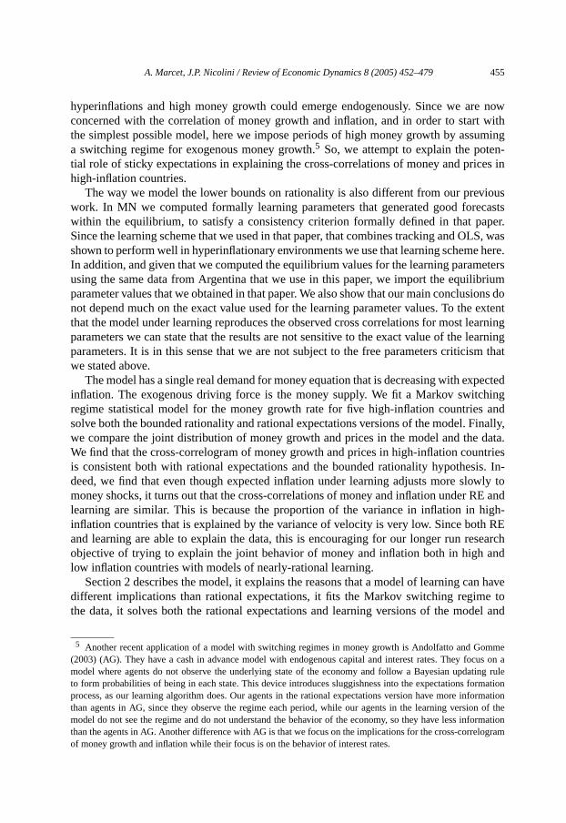
A. Marcet, J.P. Nicolini / Review of Economic Dynamics 8 (2005) 452–479 455
e nowwithumingn-es in
iouscastsper.
LS, washere.eters
briumions doextent
earninglearningsm that
pectedhingandinally,data.
ntriesis. In-wly toE and
high-h REsearchand
n havee toel and
mmecus on ating rulermationormationn of theormationlogram
hyperinflations and high money growth could emerge endogenously. Since we arconcerned with the correlation of money growth and inflation, and in order to startthe simplest possible model, here we impose periods of high money growth by assa switching regime for exogenous money growth.5 So, we attempt to explain the potetial role of sticky expectations in explaining the cross-correlations of money and prichigh-inflation countries.
The way we model the lower bounds on rationality is also different from our prevwork. In MN we computed formally learning parameters that generated good forewithin the equilibrium, to satisfy a consistency criterion formally defined in that paSince the learning scheme that we used in that paper, that combines tracking and Oshown to perform well in hyperinflationary environments we use that learning schemeIn addition, and given that we computed the equilibrium values for the learning paramusing the same data from Argentina that we use in this paper, we import the equiliparameter values that we obtained in that paper. We also show that our main conclusnot depend much on the exact value used for the learning parameter values. To thethat the model under learning reproduces the observed cross correlations for most lparameters we can state that the results are not sensitive to the exact value of theparameters. It is in this sense that we are not subject to the free parameters criticiwe stated above.
The model has a single real demand for money equation that is decreasing with exinflation. The exogenous driving force is the money supply. We fit a Markov switcregime statistical model for the money growth rate for five high-inflation countriessolve both the bounded rationality and rational expectations versions of the model. Fwe compare the joint distribution of money growth and prices in the model and theWe find that the cross-correlogram of money growth and prices in high-inflation couis consistent both with rational expectations and the bounded rationality hypothesdeed, we find that even though expected inflation under learning adjusts more slomoney shocks, it turns out that the cross-correlations of money and inflation under Rlearning are similar. This is because the proportion of the variance in inflation ininflation countries that is explained by the variance of velocity is very low. Since botand learning are able to explain the data, this is encouraging for our longer run reobjective of trying to explain the joint behavior of money and inflation both in highlow inflation countries with models of nearly-rational learning.
Section 2 describes the model, it explains the reasons that a model of learning cadifferent implications than rational expectations, it fits the Markov switching regimthe data, it solves both the rational expectations and learning versions of the mod
5 Another recent application of a model with switching regimes in money growth is Andolfatto and Go(2003) (AG). They have a cash in advance model with endogenous capital and interest rates. They fomodel where agents do not observe the underlying state of the economy and follow a Bayesian updato form probabilities of being in each state. This device introduces sluggishness into the expectations foprocess, as our learning algorithm does. Our agents in the rational expectations version have more infthan agents in AG, since they observe the regime each period, while our agents in the learning versiomodel do not see the regime and do not understand the behavior of the economy, so they have less infthan the agents in AG. Another difference with AG is that we focus on the implications for the cross-corre
of money growth and inflation while their focus is on the behavior of interest rates.
456 A. Marcet, J.P. Nicolini / Review of Economic Dynamics 8 (2005) 452–479
models
ndof
. Thisneral
e priceon int futurearning,
com-odel
rnative
can be
pect-rate
.ematictationsodel
ve this
calibrates all the parameters. Section 3 presents empirical results and compares theto the data. Section 4 concludes.
2. The model
The model consists of a demand for cash balances given by
Pt = 1
φMt + γP e
t+1, (1)
whereφ, γ are positive parameters.Pt , Mt are the nominal price level and the demafor money, andP e
t+1 is the forecast of the price level for next period. The driving forcethe model is given by the stochastic process followed by the growth rate of moneywell known money demand equation is consistent with utility maximization and geequilibrium in the context of an overlapping generations model.
To complete the model one needs to specify the way agents forecast the futurlevel. In what follows, we compare the rational expectations version with a versiwhich agents use an ad hoc algorithm that depends on past information to forecasprices. There are several ways in which one can restrict the bounded rationality, or leversion of the model to be “close” to rational expectations. For example, it has beenmon to study the conditions under which the equilibrium outcome of the learning mconverges to the rational expectations model. To be more specific, consider two alteexpectation formation mechanisms in the above money demand:
P et+1 = Et [Pt+1],
P et+1 = L(Pt ,Pt−1, . . .)
for a given functionL.6 We can then obtain corresponding solutions{P REt , P L
t }∞t=0 and,lettingρ(S1, S2) be some distance between two sequencesS1 andS2,
ρ({
P REt
}∞t=0,
{P L
t
}t=0
)(2)
measures how different the two equilibria are. Convergence to rational expectationswritten as
limt→∞
(P RE
t − P Lt
) = 0.
When this occurs, the equilibrium outcome under learning “looks like” a rational exations equilibrium in the limit. Only the transition, if long enough, can then genedifferent behavior in the rational expectations or in the learning version of the model
Near-rationality can be interpreted as imposing restrictions on the size of the systmistakes the agents make in equilibrium. This amounts to saying that agents’ expeccannot be too far away from the actual behavior of the economy or, formally, if the mis deterministic, it amounts to imposing that the distance
ρ({
P Lt
}∞t=0,
{L(Pt−1,Pt−2, . . .)
}∞t=0
)(3)
6 Strictly speaking,L could depend on the time period, as it does if agents use OLS estimates, but we lea
dependence implicit.
A. Marcet, J.P. Nicolini / Review of Economic Dynamics 8 (2005) 452–479 457
-
ns. If,small,
,nal
hat areiricalay beetric
at ef-isl ex-riumvesti-that itvior of
para-s check,oun-s littleence.encehighdatay the
he log
coun-periodata on
see theke the
cannot be too large. In an extreme case, if the functionL is such that the learning equilibrium makes zero mistakes we have that
ρ({
P Lt
}∞t=0,
{L(Pt−1,Pt−2, . . .)
}∞t=0
) = 0.
Since, by definition, rational expectations requires thatρ({P REt }∞t=0, {P e
t }∞t=0) = 0, the lastequation forces the nearly-rational learning to be the same as rational expectatioinstead, we impose that the mistakes in (3) need not be zero but that they have to bewe impose no restriction on the relationship betweenP RE
t andP Lt . As a matter of fact
in some models even ifL is restricted so that (3) is small, the difference with the ratioexpectations outcome (i.e. (2)) can be very large. There may be learning equilibria tnear-rational and whose equilibrium is vastly different from RE. In this case, the empimplications of the rational expectations version and the “small mistakes” version mdifferent, while the learning equilibrium is still close to being rational, in the proper mdefined by (3).
One example of this behavior is MN. In that paper we impose three bounds thfectively impose different metricsρ. As we mentioned in the introduction, if inflationlow, then the only learning equilibrium in MN that satisfies the bounds is the rationapectations equilibrium. However, when inflation is high, there are learning equiliboutcomes that look different from the rational expectations one. In this empirical ingation we focus the analysis on high-inflation countries only; at first sight it seemsis in these countries where it is easier to obtain large differences between the behalearning and rational expectations.
2.1. A regime switching model for money growth
In order to numerically solve the model, we will use learning and money demandmeter values that are calibrated to the Argentine economy. However, as a robustneswe will also investigate the evolution of the money supply for other high-inflation ctries. As we will see, varying either money demand or learning parameters makedifference in the results. However, the evolution of money supply does make a differ
In order to fit the process for the nominal money supply, we first look at the evidfor five Latin-American countries that experienced high average inflation and veryvolatility in the last decades: Argentina, Bolivia, Brazil, Mexico and Peru. We usefor M1 and consumer prices from the International Financial Statistics published bInternational Monetary Fund. To compute growth rates, we used the difference in tof the variable.7
While the high-inflation years are concentrated between 1975 and 1995 for mosttries, the periods do not match exactly. Thus, we chose, for each country, a sub-that roughly corresponds to its own unstable years. Figures 1(a)–(e) plot quarterly dnominal money growth and inflation for the relevant periods in each case.
7 This measure underestimates growth rates for high-inflation countries. With this scale, it is easier tomovements of inflation rates in the—relatively—tranquil periods in all the graphs. In what follows, we ma
case that the data is best described as a two-regime process, so this measure biases the result against us.
458 A. Marcet, J.P. Nicolini / Review of Economic Dynamics 8 (2005) 452–479
Fig. 1(a). Argentina.
Fig. 1(b). Bolivia.
Fig. 1(c). Brazil.

A. Marcet, J.P. Nicolini / Review of Economic Dynamics 8 (2005) 452–479 459
h, butrates,r
tern.
e, Bruno
growthes, foritchingt turned
Fig. 1(d). Mexico.
Fig. 1(e). Peru.
As it can be seen from the figures, for all those countries, average inflation was higthere are some relatively short periods of bursts in both money growth and inflationfollowed, again, by periods of stable but high-inflation rates.8 Note also that the behavioof the money growth rate, the driving force of the model, follows a very similar patThus, we propose to fit a Markov switching process for the rate of money growth.9
8 This feature of the data has long been recognized in case studies of hyperinflations (see, for examplet al., 1988).
9 Actually, data suggest that during the periods of hyperinflations, both inflation and the rate of moneyincrease over time, a fact that is consistent with the model in MN. The statistical model we fit assumsimplicity, that during the hyperinflations both have a constant mean. We tried to fit the data to a swregime model that allowed for an increasing money growth rate in the high state, but the growth elemen
out not to be statistically significant and sometimes it took the wrong sign. For this reason we decided to stay
460 A. Marcet, J.P. Nicolini / Review of Economic Dynamics 8 (2005) 452–479
h fre-ggestst that
r
en as
e
ionsultsstateslatilitywth intateimesalwaysThese
cterized
nt
n for themodel
enerateduse ae cross-does not
Our empirical analysis is based on quarterly data, since we are interested in higquency movements in money and prices. Our eyeball inspection of Figs. 1(a)–(e) suthe existence of structural breaks. This is confirmed by the breakpoint Chow Teswe present in Appendix A for the five countries, so we model� log(Mt) = log(Mt) −log(Mt−1) as a discrete time Markov switching regime process. We assume that� log(Mt)
is distributedN(µst , σ2st), wherest ∈ {0,1}. The statest is assumed to follow a first orde
Markov process with Pr(st = 1 | st−1 = 1) = q and Pr(st = 0 | st−1 = 0) = p. The evolu-tion of the first difference of the logarithm of the money supply can therefore be writt
� log(Mt) = µ0(1− st ) + µ1st + (σ0(1− st ) + σ1st
)εt
whereεt is assumed to be i.i.d. and distributedN(0,1). All empirical results regarding thmodeling of the money supply are reported in Appendix A.
One state is always characterized by higher mean and higher volatility of� log(Mt)
in all countries. Both pairs(µi, σi) are statistically significant, as well as the transitprobabilities,p andq, and both states are highly persistent in all countries. These regive very clear evidence that modeling the growth rate of money as having twois a reasonable assumption. The rate of money growth in the high-mean/high-vostate (henceforth, the “high state”) ranges from three times the rate of money grothe low state for Argentina to nine times for Bolivia while the volatility of the high sranges from one and a half times the volatility of the low state for Mexico to eight tfor Brazil. The differences across states are gigantic. The estimated high state isconsistent with the existence of high peaks of inflation in each of the countries.periods are represented as the shaded areas in Figs. 1(a)–(e).
These results clearly demonstrate that the economic environment can be charaby one in which there are changes in the monetary policy regime.
2.2. Rational expectations equilibrium
Rational expectations (RE) assumesP et+1 = Et(Pt+1) ≡ E(Pt+1 | It ) for all t , whereEt
is the expectation conditional on information up to timet . Agents observe all the relevainformation in the economy, so thatIt ≡ (Mt , st ,Pt ,Mt−1, st−1,Pt−1, . . .).
We look for non-bubble equilibria, and we conjecture that in the RE equilibrium
Et(Pt+1) = βREt Pt (4)
with βREt being state dependent and
βREt = β0(1− st ) + β1st
for some constantsβ0, β1. To solve for an equilibrium, we must find(β0, β1).
with a constant growth rate conditional on each regime. It would seem that assuming a constant meagrowth rate of money in the hyperinflation regime biases the results against our rational expectationssince, in the learning version, agents adapt to whatever data is available, while if the data indeed is gby a growing inflation in the high-inflation regime we are forcing the “rational” agents in our model tomisspecified process for the money supply. To the extent that our rational expectations model fits thcorrelogram appropriately, it seems that assuming a constant expected money growth in both states
affect our results.
A. Marcet, J.P. Nicolini / Review of Economic Dynamics 8 (2005) 452–479 461
Denote the average money growth conditional on each state byκj ≡ E(Mt+1/Mt |st+1 = j, It ). Using the fact that logMt+1/Mt ∼ N(µj ,σj ) we have that
κj = exp
(µj + 1
2σ 2
j
)(5)
and that
E
(Mt+1
Mt
∣∣∣∣ st = 0, It
)= κ0p + κ1(1− p), (6)
E
(Mt+1
Mt
∣∣∣∣ st = 1, It
)= κ0(1− q) + κ1q. (7)
The following lemma characterizes equilibrium prices.
Lemma 1. The RE equilibrium is given by
E
(Pt+1
Pt
∣∣∣∣ st = 1, It
)= β1 = κ0(1− q) + κ1q + κ0κ1γ (1− q − p)
1+ γ κ0(1− p − q),
E
(Pt+1
Pt
∣∣∣∣ st = 0, It
)= β0 = pκ0 + (1− p)κ1
1− γβ0
1− γβ1,
which gives the equilibrium price
Pt = Mt
φ(1− γβREt )
.
Proof. We have
E(Pt+1 | st = 0, It ) = pE
(Mt+1
φ(1− γβ0)
∣∣∣ st+1 = 0, st = 0, It
)
+ (1− p)E
(Mt+1
φ(1− γβ1)
∣∣∣ st+1 = 1, st = 0, It
)
= p
φ(1− γβ0)E(Mt+1 | st+1 = 0, st = 0, It )
+ (1− p)
φ(1− γβ1)E(Mt+1 | st+1 = 1, st = 0, It )
= pκ0
φ(1− γβ0)Mt + (1− p)κ1
φ(1− γβ1)Mt
= pκ0Pt + (1− p)κ1(1− γβ0)
(1− γβ1)Pt(
(1− γβ0))
= Pt pκ0 + (1− p)κ1(1− γβ1)
,

462 A. Marcet, J.P. Nicolini / Review of Economic Dynamics 8 (2005) 452–479
ining
to the
in theis notmoneyer thes
e econ-et
rent
ching
where the first equality arises from Eq. (1) and the conjectureP et+1 = E(Pt+1 | st = 0, It ) =
β0Pt . The third equality comes from (5), and the fourth comes from Eq. (1). Combthis expression with (4) we get
β0 = pκ0 + (1− p)κ11− γβ0
1− γβ1. (8)
From an analogous derivation conditioning onst = 1 we get
β1 = qκ1 + (1− q)κ01− γβ1
1− γβ0. (9)
Solve this system of equations for the unknowns(β0, β1) to get
β1 = κ0(1− q) + κ1q + κ0κ1γ (1− q − p)
1+ γ κ0(1− p − q)
and plugging this expression into (8) we obtain the solution forβ0.Plugging this into (4) and (1) we get the equilibrium prices.�Notice that expected inflation differs from expected money growth in state 0, due
presence of the factor(1− γβ0)/(1− γβ1) (or its inverse in state 1).This factor appears because under RE the inflation rate satisfies
Pt
Pt−1= 1− γβRE
t−1
1− γβREt
Mt
Mt−1,
so that if there is a change of regime from one period to the next, the ratio(1− γβREt−1)/
(1− γβREt ) introduces a wedge between the change in prices relative to the change
money supply. In this model, therefore, when there is a regime change, the velocityconstant, due to the fact that expected inflation influences the relationship betweenand prices. Notice that the difference between inflation and money growth is larglarger the difference in expected inflations, and that ifp + q = 1 the two possible valueof inflation are equal to the two possible values of money growth in each state.
2.3. Learning equilibrium
In the model under learning we assume that agents do not observe the state of thomy, they only observe inflation. We use the same learning mechanism as in MN. L
P et+1 = βtPt , (10)
where
βt = βt−1 + 1
αt
(Pt−1
Pt−2− βt−1
). (11)
The coefficientαt is called the “gain” and it affects the sensitivity of expectations to curinformation.
If we want to produce a model of learning that reproduces the observed swit
regimes and where agents are near-rational, we need to use a learning mechanism that
A. Marcet, J.P. Nicolini / Review of Economic Dynamics 8 (2005) 452–479 463
most
mentmak-gime ists usedis oc-
d belearn
redic-e that
g as thetected.
leastrameterses toply rule
ters totiver high-sitivityd them
sectionlevels of
produces reasonably low prediction errors when there is a regime switch. Two of thecommon specifications for the gain sequence are tracking (αt = α for all t), which performswell in environments that change often, and least squares(αt = αt−1 + 1), that performswell in stationary environments. What is a better learning mechanism in an environwith switching regimes, tracking or OLS? If agents used pure tracking they would being large mistakes when a state has been in place for a long time, because the renot switching and they adapt too much to money shocks. On the other hand, if agenpure OLS they would be making large mistakes after a regime switch, because if thcurred whent is relatively high, data on inflation generated by the new regime woulincorporated very slowly into expectations so that they would take a very long time toabout the new regime.
As we argue in MN a scheme that combines tracking and OLS generates good ptions overall. Since we aim at a model of learning that is nearly-rational, we assumagents combine both mechanisms so that the gain is assumed to follow OLS as lonforecast error is not large, but it switches to tracking as soon as some instability is deFormally
αt ={
αt−1 + 1 if∣∣Pt−1/Pt−2−βt−1
βt−1
∣∣ � ν,
α otherwise,(12)
whereα, ν are the learning parameters. Thus, if errors are small, the gain follows asquares rule, and as long as the regime does not switch, agents soon learn the paof the money supply rule. But if a large enough error is detected, the rule switcha constant gain algorithm, so agents can learn the new parameters of the money supfaster.
The solution{Pt/Pt−1, βt , αt } must satisfy (11), (12) and
Pt
Pt−1= 1− γβt−1
1− γβt
Mt
Mt−1,
which is obtained by plugging (10) into (1).
2.4. Calibration
As we mentioned before, we calibrate our money demand and learning paramedata from Argentina.10 As a first exploration on how the models behave with alternamoney supply processes, we also solve the model with the money supplies of otheinflation countries. This turned out to be a very reasonable exercise, since the senanalysis we did by varying the money demand and the learning parameters showenot to be very important from the quantitative point of view.
10 Note that in the current paper we focus on non-bubble equilibria. The Laffer curve mentioned in thisrefers to the fact that in our previous paper, with endogenous money supply, there were two stationary
inflation consistent with a given level of seigniorage.
464 A. Marcet, J.P. Nicolini / Review of Economic Dynamics 8 (2005) 452–479
ationse onerizedhigh,”ata on
sion,maxi-
ndingsemandmand
te
x-
above.results
stateswn withame for
model.ers of
bove.n-matic
rameter
Money demandWe borrow the parameter values from our previous paper, in which we use observ
from empirical Laffer curves to calibrate them. This is a reasonable choice: sincempirical implication of the original model is that recurrent hyperinflations characteby two regimes occur when average inflation—driven by average seigniorage—is “we need to have a benchmark to discuss what “high” means. We use quarterly dinflation rates and seigniorage as a share of GNP for Argentina11 from 1980 to 1990 fromAhumada et al. (1993) to fit an empirical Laffer curve. While there is a lot of disperthe maximum observed seigniorage is around 5% of GNP, and the inflation rate thatmizes seigniorage is close to 60%. These figures are roughly consistent with the fiin Kiguel and Neumeyer (1995) and other studies. The parameters of the money dγ andφ, are uniquely determined by the two numbers above. Note that the money defunction implies a stationary Laffer curve equal to
π
1+ πm = π
1+ πφ(1− γ (1+ π)
)(13)
wherem is the real quantity of money andπ is the inflation rate. Thus, the inflation rathat maximizes seigniorage is
π∗ =√
1
γ− 1
which, settingπ∗ = 60%, impliesγ = 0.4. Using this figure in (13), and making the maimum revenue equal to 0.05, we obtainφ = 0.37.
Money supplyFor money supply, we use the estimated Markov switching models we discussed
We fit this process to the observed behavior of money supply to each country. Theof the estimation are reported in Appendix A. We use the estimated parameters andas the true values of the exogenous process, and we assume that these are knocertainty by the agents. While the money demand parameters are assumed the seach country, the money supply process is estimated using data from each country.
Learning parametersThe parameters described above are sufficient to solve the rational expectations
However, we still need to be specific regarding our choice of the (still free!) parametthe learning process,α, ν.
In MN, we provided an operational definition of a bound of the type described aIn that paper we searched for values of the parameterα that satisfy a rational expectatiolike, approximate fixed point problem so that, in equilibrium, agents make small systemistakes. In this paper we use the equilibrium values we obtained in MN (α between 2and 4) and we show the robustness of the results we obtain to the choice of these pa
11 The choice of country is arbitrary. We chose Argentina because we were more familiar with the data.

A. Marcet, J.P. Nicolini / Review of Economic Dynamics 8 (2005) 452–479 465
hly
manden thee ra-rium
of themar-oney
Therees insis ofcon-
h) istweenrelationand (b)for thelatedre thetheother
e esti-for the4. Theunderof the
) given norted byically
e
the
relations
values. For the value ofν, we also follow MN, where we used a value that was rougequal to two standard deviations of the prediction error.12
3. Evaluating the models
The main goal of this paper is to investigate the ability of the standard money demodel with exogenous money growth to replicate the short-run relationship betweinflation rate and the growth rate of money in high-inflation countries, using both thtional expectations model and the “almost” rational version. We dub LM the equilibunder the learning mechanism.
Following the RBC tradition, we characterize the data using empirical momentsjoint distribution of money growth and prices. Table A.3 presents moments of theirginal distributions. As one should expect, average inflation is very similar to average mgrowth in each country (see, for example, Lucas, 1980 for a discussion of this fact).are slightly larger differences between the volatility of inflation and money growth rateach country, without a clear pattern emerging from the table. We will focus our analythe joint distribution of money and prices on the cross-correlogram. If velocity were astant fraction of output, in countries where the volatility of inflation (and money growtmuch larger than the volatility of output growth, the contemporaneous correlation bemoney and prices ought to be close to one, and the leads and lags of the cross-corshould be equal to the auto-correlogram of the money growth process. Figures 2(a)present the leads and lags for the cross-correlation of money growth and pricesfive countries. It is interesting to point out that money and prices are highly correcontemporaneously, contrary to the case of middle and low inflation countries whecorrelation is less strong.13 In particular, the contemporaneous correlation for Mexico,country in the sample with lower average inflation, is substantially lower than for thecountries.
We simulate the model using the calibrated parameters for money demand, thmated values for the money supply process, and we plug in the observed valuesmoney supply. The results of the simulations are shown in Table B.1 and Figs. 3 andcolumns of Table B.1 show the moments for the inflation generated by the modelrational expectations, and under LM. Under LM we have two columns, one for eachtwo possible values forα = {10/4,10/3}.
As we can see, the three simulations (the one under RE and the two under LMvery similar results for each of the countries. In fact, for Argentina, neither the meathe standard deviation of the RE model are statistically different from the ones generathe two different versions of LM. Most importantly, none of these moments are statist
12 We also solved the learning model with an alternative specification forv, given the Markov structure of thmoney growth process: we replacev for vst , where, ifst = 1 is the state with the higher growth, we havevl = v
andv1 = (σh/σl)v. With this alternative specification we introduce the switching regime information intolearning mechanism, but it did not make any difference in the results.13 See Alvarez et al. (2001) and references therein for theoretical work that aims at matching these cor
for low inflation countries.
466 A. Marcet, J.P. Nicolini / Review of Economic Dynamics 8 (2005) 452–479
Fig. 2(a). Lead:�— Argentina,�— Bolivia, �— Brazil, — Mexico,×— Peru.
Fig. 2(b). Lag:�— Argentina,�— Bolivia, �— Brazil, — Mexico,×— Peru.

A. Marcet, J.P. Nicolini / Review of Economic Dynamics 8 (2005) 452–479 467
Fig. 3(a). Argentina: lag with confidence bands: — Data,�— LM1, ×— LM, �— RE.
Fig. 3(b). Bolivia: lag with confidence bands: — Data,�— LM1, �— LM, ×— RE.

468 A. Marcet, J.P. Nicolini / Review of Economic Dynamics 8 (2005) 452–479
Fig. 3(c). Brazil: lag with confidence bands: — Data,�— LM1, �— LM, ×— RE.
Fig. 3(d). Mexico: lag with confidence bands: — Data,�— LM1, �— LM, ×— RE.

A. Marcet, J.P. Nicolini / Review of Economic Dynamics 8 (2005) 452–479 469
Fig. 3(e). Peru: lag with confidence bands: — Data,�— LM1, �— LM, ×— RE.
Fig. 4(a). Argentina: lead with confidence bands: — Data,×— LM1, �— LM, �— RE.

470 A. Marcet, J.P. Nicolini / Review of Economic Dynamics 8 (2005) 452–479
Fig. 4(b). Bolivia: lead with confidence bands: — Data,�— LM1, �— LM, ×— RE.
Fig. 4(c). Brazil: lead with confidence bands: — Data,�— LM1, �— LM, ×— RE.

A. Marcet, J.P. Nicolini / Review of Economic Dynamics 8 (2005) 452–479 471
Fig. 4(d). Mexico: lead with confidence bands: — Data,�— LM1, �— LM, ×— RE.
Fig. 4(e). Peru: lead with Confidence bands: — Data,�— LM1, �— LM, ×— RE.

472 A. Marcet, J.P. Nicolini / Review of Economic Dynamics 8 (2005) 452–479
andtionwhilete the
l and
am be-e fornd,
ry sim-ed bypec-
eablein themma 1,rowth,thisuntryns are
orane-hichlogram.
on arein
to theexico.eemedls are
ratio-rningre 5d
hat ex-tionalwever,sug-
ts
different from the actual moments of inflation. The same is true for Peru, BoliviaMexico. Similar results arise for Brazil, with the exception that the volatility of the inflarate under learning overestimates the true volatility. It is interesting to point out thatthe simulations for Argentina, Bolivia and Peru generate volatilities that underestimaactual ones, the volatility in the model overestimates the actual volatility for BraziMexico.
Figures 3(a)–(e) and 4(a)–(e) present the leads and lags of the cross-correlogrtween log(Mt/Mt−1) and the inflation rates generated by RE, LM and the actual oneach of the five countries.14 We also include an approximation for the confidence ba(±2/
√T ) for the cross-correlogram of the actual series (the dotted lines).
For each country, the cross-correlogram generated with the three models are veilar. Again, with the exception of Mexico, none of the cross-correlograms generateither model is significantly different from the actual one. Learning and rational extations perform equally well in approximating the actual cross-correlogram. A noticfact is that in every country except Mexico the contemporaneous correlation is lowersimulated series than in the actual ones. This is because, as we pointed out after Lethe two states of expected inflation do not match the two states of expected money gand velocity in the model is not equal to one; since LM looks fairly close to RE inmodel, the same occurs in the learning model. The only exception is Mexico, the cowith the lowest average inflation, where the simulated contemporaneous correlatiostill close to one but the actual correlation is less than 0.5 (obviously, the contempous correlation is the intercept in Fig. 3). Furthermore, Mexico is the only country wpresents significant differences between the actual and the simulated cross-correThis is due to the fact that Mexico’s actual inflation is not so correlated to log(Mt/Mt−1)
as it is in the other countries (shown in Figs. 1(a)–(e)), and as the simulated inflatihighly correlated to log(Mt/Mt−1) they perform worse for this particular case. But eventhe case of Mexico the prediction of the money demand model is not very sensitiveexpectation formation mechanism: the three models perform equally less well for M
The most important conclusion of the paper is that, although sticky expectations sa good candidate to obtain different behavior from rational expectations, the modeempirically equivalent if the money supply is forced to behave like in the data.
This is not because we forced the learning model to be artificially close to thenal expectations model by imposing very high rationality requirements in the leamodel. In fact, both models do imply different behavior for expected inflation. Figuplots expected inflation for the case of Argentina.15 BETAdenotes expected inflation anthe labels are the same as previous figures, thusBETA LMandBETA LM1 correspond tothe expected inflation in the learning model forα equal to 10/3 and 10/4, while BETAREstands for the expected inflation under rational expectations. The figure shows tpected inflation under learning exhibits stronger high frequency movements than raexpectations. Thus the real money demand also moves more under learning. Hothe impact on the behavior of the cross correlogram is quantitatively small. This
14 More precisely, for each model or data, the entry corresponding toj in the horizontal axis of Figs. 3 represencorr(log(Mt /Mt−1), log(Pt−j /Pt−j−1)).
15 The same happens in the other five countries.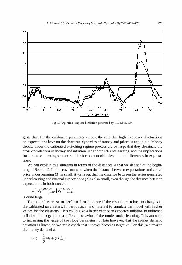
A. Marcet, J.P. Nicolini / Review of Economic Dynamics 8 (2005) 452–479 473
ationsoney
ate theationspecta-
-actual
neratedetween
ges inigher
uenceountsndrewrite
Fig. 5. Argentina. Expected inflation generated by RE, LM1, LM.
gests that, for the calibrated parameter values, the role that high frequency fluctuon expectations have on the short run dynamics of money and prices is negligible. Mshocks under the calibrated switching regime process are so large that they domincross-correlations of money and inflation under both RE and learning, and the implicfor the cross-correlogram are similar for both models despite the differences in extions.
We can explain this situation in terms of the distancesρ that we defined at the beginning of Section 2. In this environment, when the distance between expectations andprice under learning (3) is small, it turns out that the distance between the series geunder learning and rational expectations (2) is also small, even though the distance bexpectations in both models
ρ({
Pe,REt
}∞t=0,
{P
e,Lt
}∞t=0
)is quite large.
The natural exercise to perform then is to see if the results are robust to chanthe calibrated parameters. In particular, it is of interest to simulate the model with hvalues for the elasticity. This could give a better chance to expected inflation to inflinflation and to generate a different behavior of the model under learning. This amto increasing the value of the slope parameterγ . Note however, that the money demaequation is linear, so we must check that it never becomes negative. For this, wethe money demand as
1 e
δPt =φMt + γPt+1.

474 A. Marcet, J.P. Nicolini / Review of Economic Dynamics 8 (2005) 452–479
money, sinced. Thecheck
aluesd therenes of
is in-tion ismp. Asdel thee last
1990
oneytationfits thef this
ex-ces incouldn lowtionior in
posingecha-
s thatmodel
Table 1Correlation between observed and predicted inflation for the two models
γ 0.4 0.45 0.5 0.55 0.6
Corr(True Inf, Inf LM) 80.85 80.57 80.36 80.19 79.69Corr(True Inf, Inf RE) 78.12 76.54 73.98 69.92 63.57
Thus, when increasing the value forγ , we also increased the value forδ such that themoney demand was always positive. Note that we are changing the values for thedemand keeping fixed the learning parameters. This is not an equilibrium exercisethe equilibrium values for the learning parameters do depend on the money demanonly purpose of this exercise is to amplify the effects of the sluggish expectations andif they go in the direction of better explaining the data. We solved the model for vof γ between 0.4 and 0.6. The auto-correlograms were already on the target anwas no noticeable difference by changing the values ofγ . Table 1 reports the correlatiobetween the inflation rate and the inflation predicted by the model for different valuthe parameterγ .
The performance of the two models gets poorer as the value of the elasticitycreased. It does worst for the RE model. The reason is that with RE, expected inflaa step function. Therefore, as the regime changes, the price level makes a larger juobserved inflation is a smoother series, the correlation worsens. For the learning mocorrelations do not change much. They get (mildly) worse mainly because after thhyperinflation of Argentina in 1989 the model predicts a sharper drop in inflation inthan the one that actually occurred as the elasticity gets bigger.
This exercise reinforces the conclusion that for the high-inflation economies, our mdemand model gives a small role to the behavior of expectations. A possible limiof our analysis is the linear money demand used, which is not the one that bestevidence. However, exploring with log linear specifications is far beyond the scope opaper.
4. Conclusion
The purpose of this paper is to explore the potential role of “nearly-rational”pectations in explaining the high frequency movements between money and prihigh-inflation countries. Sluggish expectations imply movements on velocity thatpotentially explain the observed sluggish response of inflation to money shocks iinflation countries. But the correlation of inflation and money growth in high-inflacountries is quite high. The fact that rational expectations can explain this behavhigh-inflation countries poses a challenge to models of learning.
We use a learning mechanism that produces good forecasts within the model, iman approximate rational expectations requirement. This insures that the learning mnism introduced in the model is not arbitrarily chosen to match the data and it insurethe agents are not making obvious mistakes in the model. We argue that the learning
we propose is nearly rational in countries where monetary policy exhibits frequent and sub-
A. Marcet, J.P. Nicolini / Review of Economic Dynamics 8 (2005) 452–479 475
rivingencend wens and
iricalon forust tovior oftationsgrowthtionalhigh-
ousrcet ac-roject
pro-icolini
.
ation.de
th
stantial changes of regime. We fit a Markov switching process for the exogenous dforce—the money growth rate—to five Latin-American countries. There is ample evidin favor of the regime switching structure. We calibrate a money demand equation astudy the solutions of the model under the assumptions of both rational expectatiolearning.
We find that both learning and rational expectations generate very similar empimplications that match the observed cross-correlogram of money growth and inflatithe high-inflation countries considered in almost every dimension. This result is robincreasing the elasticity of money demand. Thus, we conclude, the short run behamoney and prices in high-inflation countries can be explained both by rational expecand learning models. This is encouraging, because the high correlation of moneyand inflation observed in high-inflation countries does not need the assumption of raexpectations, so it leaves room for models of learning to explain the behavior of bothand low-inflation countries.
Acknowledgments
We want to thank Rodi Manuelli, Andy Neumeyer, Mike Woodford and an anonymreferee for comments, and Demian Pouzo for excellent research assistance. Maknowledges financial support from the Ministerio de Ciencia y Technologia, Spain pDGES SEC2002-01601, CIRIT, Catalonia, CREI, and Barcelona Economics with itsgram CREA. Part of this research was done when Marcet was a visitor at the ECB. Nacknowledges financial support from ANCT, Argentina.
Appendix A. Empirical results
A.1. Chow Test for structural breaks
The Chow Test for the corresponding sub-samples generates results in Table A.1
A.2. Markov Switching Regime estimation results
In this subsection we present the results of the Markov Switching Regimes estimLet p = Pr(st = 0 | st−1 = 0), q = Pr(st = 1 | st−1 = 1), and letµi andσi be the mean anthe standard deviation of the growth rate of money in statei. Table A.2 summarizes thresults of the estimation.
A.3. First and second moments
Table A.3 shows the first(µ) and second(σ ) moments of inflation and money grow
for every country.
476 A. Marcet, J.P. Nicolini / Review of Economic Dynamics 8 (2005) 452–479
Table A.1
Probability
Argentina (1975:01–1992:04)Sub-samples: 1975:01–1988:04, 1989:01–1990:01, 1990:02–1992:04Chow breakpoint test: 1989:01–1990:01F -statistic 3.7752 0.0029Log likelihood ratio 22.0998 0.0011
Bolivia (1975:01–1995:04)Sub-samples: 1975:01–1983:03, 1983:04–1986:04, 1987:01–1995:04Chow breakpoint test: 1983:04–1986:04F -statistic 4.2050 0.0034Log likelihood ratio 16.4706 0.0024
Brazil (1980:01–1995:04)Sub-samples: 1980:01–1987:04, 1988:01–1991:01, 1991:02–1995:04Chow breakpoint test: 1988:01–1991:01F -statistic 4.6664 0.0017Log likelihood ratio 18.1274 0.0011
Mexico (1975:01–1995:04)Sub-samples: 1975:01–1989:04, 1990:01–1992:03, 1992:04–1995:04Chow breakpoint test: 1990:01–1992:03F -statistic 4.2514 0.0032Log likelihood ratio 16.6383 0.0022
Peru (1975:01–1995:04)Sub-samples: 1975:01–1989:04, 1990:01–1991:01, 1991:02–1995:04Chow breakpoint test: 1990:01–1991:01F -statistic 16.6757 0.0000Log likelihood ratio 53.9042 0.0000
Table A.2
Coeff. Std. error t-statistic
Argentina (1975:01–1992:04)µ0 0.1755 0.0182 9.5933µ1 0.4543 0.0986 4.6046q 0.9150 0.0662 13.8213p 0.9193 0.0740 12.4184σ0 0.0728 0.0119 6.1000σ1 0.3034 0.0797 3.8050
Bolivia (1975:01–1995:04)µ0 0.0596 0.0097 6.1130µ1 0.5363 0.4208 1.2744q 0.9351 0.0665 14.0553p 0.9866 0.0701 14.0658σ0 0.0505 0.0037 13.5993σ1 0.3739 0.1595 2.3435
Brazil (1980:01–1995:04)µ0 0.1579 0.0276 5.7126µ1 0.5173 0.1287 4.0181
(continued on next page)

A. Marcet, J.P. Nicolini / Review of Economic Dynamics 8 (2005) 452–479 477
Table A.2 (continued)
Coeff. Std. error t-statistic
q 0.9260 0.1251 7.4018p 0.9572 0.0685 13.9568σ0 0.0454 0.0193 2.3526σ1 0.3896 0.0896 4.3468
Mexico (1975:01–1995:04)µ0 0.0646 0.0101 6.3527µ1 0.2063 0.0219 9.3930q 0.7333 0.1748 4.1948p 0.9518 0.0603 15.7802σ0 0.0476 0.0111 4.2621σ1 0.0610 0.0253 2.4044
Peru (1975:01–1995:04)µ0 0.1193 0.0150 7.9106µ1 0.7440 0.1904 3.9853q 0.8308 0.1263 6.5670p 0.9717 0.0483 19.8607σ0 0.0820 0.0086 10.0684σ1 0.3833 0.1349 2.8475
Table A.3
Sample Country Inflation Money growth(� logPt ) (� logMt)
µ σ µ σ
1975:01–1992:04 Argentina 0.328 0.301 0.305 0.2711975:01–1995:04 Bolivia 0.160 0.305 0.163 0.2701980:01–1995:04 Brazil 0.340 0.301 0.338 0.3451975:01–1995:04 Mexico 0.084 0.070 0.086 0.0731975:01–1995:04 Peru 0.225 0.309 0.217 0.290
Appendix B. Simulation results
Table B.1 shows the first and second moments of the simulations.
Table B.1
Country Sample µ σ
Argentina 1975:01–1992:04 True 0.328 0.301α = 10
3 0.331 0.294
α = 104 0.330 0.312
RE 0.330 0.273
Bolivia 1975:01–1995:04 True 0.160 0.305α = 10
3 0.167 0.305
α = 104 0.167 0.325
RE 0.167 0.274
(continued on next page)
478 A. Marcet, J.P. Nicolini / Review of Economic Dynamics 8 (2005) 452–479
sto infla-
. Journal
entory
44 (1),
roach.
l, Ar-
rtation.
. Federal
ss.veland
merican
dit and
0 (De-
mber).Theorye Univ.
erly Re-
my 92,
Table B.1 (continued)
Country Sample µ σ
Brazil 1980:01–1995:04 True 0.340 0.301α = 10
3 0.332 0.375
α = 104 0.321 0.392
RE 0.333 0.351
Mexico 1975:01–1995:04 True 0.084 0.070α = 10
3 0.086 0.077
α = 104 0.086 0.078
RE 0.087 0.076
Peru 1975:01–1995:04 True 0.225 0.309α = 10
3 0.220 0.307
α = 104 0.220 0.318
RE 0.221 0.292
References
Ahumada, H., Canavese, A., Sanguinetti, P., Sosa Escudero, W., 1993. Efectos distributivos del impuecionario: una estimación del caso argentino. Economía Mexicana, 329–385.
Alvarez, F., Atkenson, A., 1997. Money and exchange rates in the Grossman–Weiss–Rotemberg modelof Monetary Economics 40 (3), 619–640.
Alvarez, F., Atkenson, A., Edmond, C., 2001. On the sluggish response of prices to money in an invtheoretic model of money demand. Working paper. UCLA.
Andolfatto, D., Gomme, P., 2003. Monetary policy regimes and beliefs. International Economic Review1–30.
Arifovic, J., Bullard, J., Duffy, J., 1997. The transition from stagnation to growth: an adaptive learning appJournal of Economic Growth 2, 185–209.
Bruno, M., Di Tella, G., Dornbusch, R., Fisher, S., 1988. Inflation Stabilization. The Experience of Israegentina, Brazil and Mexico. MIT Press.
Chung, H.-T., 1990. Did policy makers really believe in the Phillips curve? An econometric test. PhD disseUniversity of Minnesota.
Evans, G.W., Honkapohja, S., 1993. Adaptive forecasts and hysteresis, and endogenous fluctuationsReserve Bank of San Francisco Economic Review 1.
Evans, G.W., Honkapohja, S., 2001. Learning and Expectations in Macroeconomics. Princeton Univ. PreFitzgerald, T., 1999. Money growth and inflation, how long is the long run? Federal Reserve Bank of Cle
Economic Commentary (August).Grossman, S., Weiss, L., 1983. A transactions-based model of the monetary transmission mechanism. A
Economic Review 73, 871–880.Kiguel, M., Neumeyer, P.A., 1995. Inflation and seigniorage: the case of Argentina. Journal of Money Cre
Banking 27 (3), 672–682.Lucas Jr., R.E., 1980. Two illustrations on the quantity theory of money. American Economic Review 7
cember), 1005–1014.Marcet, A., Nicolini, J.P., 2003. Recurrent hyperinflations and learning. American Economic Review (DeceMarimon, R., 1997. Learning from learning in economics. In: Advances in Economics and Econometrics:
and Applications. Invited Sessions at The 7th World Congress of the Econometric Society. CambridgPress.
McCandless, G., Weber, W., 1995. Some monetary facts. Federal Reserve Bank of Minneapolis Quartview 19 (3), 2–11.
Rotemberg, J., 1984. A monetary equilibrium model with transactions costs. Journal of Political Econo
40–58.
A. Marcet, J.P. Nicolini / Review of Economic Dynamics 8 (2005) 452–479 479
ité de
excess
Saint-Paul, G., 2001. Some evolutionary foundations for price level rigidity. Working paper. UniversToulouse.
Sargent, T.J., 1993. Bounded Rationality in Macroeconomics. Oxford Univ. Press.Sargent, T.J., 1999. The Conquest of American Inflation. Princeton Univ. Press.Timmermann, A., 1993. How learning in financial markets generates excess volatility and predictability of
returns. Quarterly Journal of Economics 108, 1135–1145.