Embed Size (px)
Citation preview

Chapter 9
Monetary Policy andNominal Exchange RateDetermination
Thus far, we have focused on the determination of real variables, such asconsumption, the trade balance, the current account, and the real exchangerate. In this chapter, we study the determination of nominal variables, suchas the nominal exchange rate, the price level, inflation, and the quantity ofmoney.
We will organize ideas around using a theoretical framework (model)that is similar to the one presented in previous chapters, with one importantmodification: there is a demand for money.
An important question in macroeconomics is why households voluntarilychoose to hold money. In the modern world, this question arises becausemoney takes the form of unbacked paper notes printed by the government.This kind of money, one that the government is not obliged to exchange forgoods, is called fiat money. Clearly, fiat money is intrinsically valueless. Onereason why people value money is that it facilitates transactions. In the ab-sence of money, all purchases of goods must take the form of barter. Barterexchanges can be very difficult to arrange because they require double co-incident of wants. For example, a carpenter who wants to eat an ice creammust find an ice cream maker that is in need of a carpenter. Money elimi-nates the need for double coincidence of wants. In this chapter we assumethat agents voluntarily hold money because it facilitates transactions.
143

144 S. Schmitt-Grohe and M. Uribe
9.1 The quantity theory of money
What determines the level of the nominal exchange rate? Why has the Eurobeen depreciating vis-a-vis the US dollar since its inception in 1999? Thequantity theory of money asserts that a key determinant of the exchangerate is the quantity of money printed by central banks.
According to the quantity theory of money, people hold a more or lessstable fraction of their income in the form of money. Formally, letting Ydenote real income, Md money holdings, and P the price level (i.e., the priceof a representative basket of goods), then
Md = κP · YThis means that the real value of money, Md/P , is determined by the levelof real activity of the economy. Let md ≡ Md/P denote the demand forreal money balances. The quantity theory of money then maintains thatmd is determined by nonmonetary or real factors such as aggregate output,the degree of technological advancement, etc.. Let Ms denote the nominalmoney supply, that is, M s represents the quantity of bills and coins in cir-culation plus checking deposits. Equilibrium in the money market requiresthat money demand be equal to money supply, that is,
M s
P= md (9.1)
A similar equilibrium condition has to hold in the foreign country. Let M∗s
denote the foreign nominal money supply, P ∗ the foreign price level, andm∗d the demand for real balances in the foreign country. Then,
M∗s
P ∗ = m∗d (9.2)
Let E denote the nominal exchange rate, defined as the domestic-currencyprice of the foreign currency. So, for example, if E refers to the dollar/euroexchange rate, then stands for the number of US dollars necessary to pur-chase one euro. Let e denote the real exchange rate. As explained in previouschapters, e represents the relative price of a foreign basket of goods in termsof domestic baskets of goods. Formally,
e =E P ∗
P
Using this expression along with (9.1) and (9.2), we can express the nominalexchange rate, E, as
E =M
M∗
(e m∗
m
)(9.3)
International Macroeconomics, Chapter 9 145
According to the quantity theory of money, not only m and m∗ but alsoe are determined by non-monetary factors. The quantity of money, in turn,depends on the exchange rate regime maintained by the respective centralbanks. There are two polar exchange rate arrangements: flexible and fixedexchange rate regimes.
9.1.1 Floating (or Flexible) Exchange Rate Regime
Under a floating exchange rate regime, the market determines the nominalexchange rate E. In this case the level of the money supplies in the domesticand foreign countries, M s and M∗s, are determined by the respective centralbanks and are, therefore, exogenous variables. Exogenous variables are thosethat are determined outside of the model. By contrast, the nominal exchangerate is an endogenous variable in the sense that its equilibrium value isdetermined within the model.
Suppose, for example, that the domestic central bank decides to increasethe money supply M s. It is clear from equation (9.3) that, all other thingsconstant, the monetary expansion in the home country causes the nominalexchange rate E to depreciate by the same proportion as the increase in themoney supply. (i.e., E increases). The intuition behind this effect is simple.An increase in the quantity of money of the domestic country increases therelative scarcity of the foreign currency, thus inducing an increase in therelative price of the foreign currency in terms of the domestic currency, E.In addition, equation (9.1) implies that when M increases the domestic pricelevel, P , increases in the same proportion as M . An increase in the domesticmoney supply generates inflation in the domestic country. The reason forthis increase in prices is that when the central bank injects additional moneybalances into the economy, households find themselves with more moneythan they wish to hold. As a result households try to get rid of the excessmoney balances by purchasing goods. This increase in the demand for goodsdrives prices up.
Suppose now that the real exchange rate depreciates, (that is e goesup). This means that a foreign basket of goods becomes more expensiverelative to a domestic basket of goods. A depreciation of the real exchangerate can be due to a variety of reason, such as a terms-of-trade shock orthe removal of import barriers. If the central bank keeps the money supplyunchanged, then by equation (9.3) a real exchange rate depreciation causesa depreciation (an increase) of the nominal exchange rate. Note that e andE increase by the same proportion. The price level P is unaffected becauseneither M nor m have changed (see equation (9.1)).

146 S. Schmitt-Grohe and M. Uribe
9.1.2 Fixed Exchange Rate Regime
Under a fixed exchange rate regime, the central bank determines E by inter-vening in the money market. So given E, M∗s, and em∗s/ms, equation (9.3)determines what M s ought to be in equilibrium. Thus, under a fixed ex-change rate regime, M s is an endogenous variable, whereas E is exogenouslydetermined by the central bank.
Suppose that the real exchange rate, e, experiences a depreciation. Inthis case, the central bank must reduce the money supply (that is, Ms mustfall) to compensate for the real exchange rate depreciation. Indeed, themoney supply must fall by the same proportion as the real exchange rate.In addition, the domestic price level, P , must also fall by the same proportionas e in order for real balances to stay constant (see equation (9.1)). Thisimplies that we have a deflation, contrary to what happens under a floatingexchange rate policy.
9.2 Fiscal deficits and the exchange rate
The quantity theory of money provides a simple and insightful view of therelationship between money, prices, the nominal exchange rate, and realvariables. However, it leaves a number of questions unanswered. For exam-ple, what is the effect of fiscal policy on inflation? What role do expectationsabout future changes in monetary and fiscal policy play for the determina-tion of prices, exchange rates and real balances? To address these questions,it is necessary to use a richer model; one that incorporates a more realisticmoney demand specification and one that explicitly considers the relation-ship between monetary and fiscal policy.
In this section, embed a money demand function into a model with agovernment sector similar to the one used in chapter 4 to analyze the effectsof fiscal deficits on the current account. Specifically, we consider a small-open endowment economy with free capital mobility, a single traded good perperiod, and a government that levies lump-sum taxes to finance governmentpurchases. For simplicity, we assume that there is no physical capital andhence no investment. Domestic output is given as an endowment. Besidesthe introduction of money demand, a further difference with the economystudied in chapter 4 is that now the economy is assumed to exist not just for2 periods but for an infinite number of periods. Such an economy is calledan infinite horizon economy.
We discuss in detail each of the four building blocks that compose ourmonetary economy: (1) The money demand; (2) Purchasing power parity;

International Macroeconomics, Chapter 9 147
(3) Interest rate parity; and (4) The government budget constraint.
9.2.1 Money demand
In the quantity theory, money demand is assumed to depend only on thelevel of real activity. In reality, however, the demand for money also dependson the nominal interest rate. In particular money demand is decreasingin the nominal interest rate. The reason is that money is a non-interest-bearing asset. As a result, the opportunity cost of holding money is thenominal interest rate on alternative interest-bearing liquid assets such astime deposits, government bonds, and money market mutual funds. Thus,the higher the nominal interest rate the lower is the demand for real moneybalances. Formally, we assume a money demand function of the form:
Mt
Pt= L(C, it), (9.4)
where C denotes consumption and it denotes the domestic nominal interestrate in period t. The function L is increasing in consumption and decreasingin the nominal interest rate. We assume that consumption is constant overtime. Therefore C does not have a time subscript. We indicate that con-sumption is constant by placing a bar over C. The money demand functionL(·, ·) is also known as the liquidity preference function. Those readers in-terested in learning how a money demand like equation (9.4) can be derivedfrom the optimization problem of the household should consult the appendixto this chapter.
9.2.2 Purchasing power parity (PPP)
Because in the economy under consideration there is a single traded goodand no barriers to international trade, purchasing power parity must hold.Let Pt be the domestic currency price of the good in period t, P ∗
t the foreigncurrency price of the good in period t, and Et the nominal exchange ratein period t, defined as the price of one unit of foreign currency in terms ofdomestic currency. Then PPP implies that in any period t
Pt = EtP∗t
For simplicity, assume that the foreign currency price of the good is constantand equal to 1 (P ∗
t = 1 for all t). In this case, it follows from PPP that thedomestic price level is equal to the nominal exchange rate,
Pt = Et. (9.5)
148 S. Schmitt-Grohe and M. Uribe
Using this relationship, we can write the liquidity preference function (9.4)as
Mt
Et= L(C, it), (9.6)
9.2.3 The interest parity condition
In this economy, there is no uncertainty and free capital mobility. Thus, thegross domestic nominal interest rate must be equal to the gross world nomi-nal interest rate times the expected gross rate of devaluation of the domesticcurrency. This relation is called the uncovered interest parity condition. For-mally, let Ee
t+1 denote the nominal exchange rate that agents expect at timet to prevail at time t + 1, and let it denote the domestic nominal interestrate, that is, the rate of return on an asset denominated in domestic cur-rency and held from period t to period t + 1. Then the uncovered interestparity condition is:
1 + it = (1 + r∗)Ee
t+1
Et(9.7)
In the absence of uncertainty, the nominal exchange rate that will prevailat time t + 1 is known at time t, so that Ee
t+1 = Et+1. Then, the uncoveredinterest parity condition becomes
1 + it = (1 + r∗)Et+1
Et(9.8)
This condition has a very intuitive interpretation. The left hand side isthe gross rate of return of investing 1 unit of domestic currency in a do-mestic currency denominated bond. Because there is free capital mobility,this investment must yield the same return as investing 1 unit of domesticcurrency in foreign bonds. One unit of domestic currency buys 1/Et unitsof the foreign bond. In turn, 1/Et units of the foreign bond pay (1+ r∗)/Et
units of foreign currency in period t + 1, which can then be exchanged for(1 + r∗)Et+1/Et units of domestic currency.1
1Here two comments are in order. First, in chapter 5, we argued that free capitalmobility implies that covered interest rate parity holds. The difference between coveredand uncovered interest rate parity is that covered interest rate parity uses the forwardexchange rate Ft to eliminate foreign exchange rate risk, whereas uncovered interest rateparity uses the expected future spot exchange rate, Ee
t+1. In general, Ft and Eet+1 are
not equal to each other. However, under certainty Ft = Eet+1 = Et+1, so covered and
uncovered interest parity are equivalent. Second, in chapter 5 we further argued that
International Macroeconomics, Chapter 9 149
9.2.4 The government budget constraint
The government has three sources of income: tax revenues, Tt, money cre-ation, Mt−Mt−1, and interest earnings from holdings of international bonds,Etr
∗Bgt−1, where Bg
t−1 denotes the government’s holdings of foreign currencydenominated bonds carried over from period t − 1 into period t and r∗ isthe international interest rate. Government bonds, Bg
t , are denominated inforeign currency and pay the world interest rate r∗. The government allo-cates its income to finance government purchases, PtGt, where Gt denotesreal government consumption of goods in period t, and to changes in itsholdings of foreign bonds, Et(B
gt −Bg
t−1). Thus, in period t, the governmentbudget constraint is
Et(Bgt − Bg
t−1) + PtGt = Tt + (Mt − Mt−1) + Etr∗Bg
t−1
The left hand side of this expression represents the government’s uses ofrevenue and the right hand side the sources. Note that Bg
t is not restrictedto be positive. If Bg
t is positive, then the government is a creditor, whereasif it is negative, then the government is a debtor.2 We can express thegovernment budget constraint in real terms by dividing the left and righthand sides of the above equation by the price level Pt. After rearrangingterms, the result can be written as
Bgt − Bg
t−1 =Mt − Mt−1
Pt−
[Gt − Tt
Pt− r∗Bg
t−1
](9.9)
The first term on the right hand side measures the government’s real revenuefrom money creation and is called seignorage revenue,
seignorage revenue =Mt − Mt−1
Pt.
The second term on the right hand side of (9.9) is the difference betweengovernment expenditures and income from the collection of taxes and frominterest payments on interest-bearing assets. This term is called real sec-ondary deficit and we will denote it by DEFt,
DEFt = (Gt − Tt/Pt)− r∗Bgt−1
free capital mobility implies that covered interest parity must hold for nominal interestrates. However, in equation (9.7) we used the world real interest rate r∗. In the contextof our model this is okay because we are assuming that the foreign price level is constant(P ∗ = 1) so that, by the Fisher equation (5.3), the nominal world interest rate must beequal to the real world interest rate (i∗t = r∗t ).
2Note that the notation here is different from the one used in chapter 4, where Bgt
denoted the level of government debt.
150 S. Schmitt-Grohe and M. Uribe
The difference between government expenditures and tax revenues (Gt −Tt/Pt) is called primary deficit. Thus, the secondary government deficitequals the difference between the primary deficit and interest income fromgovernment holdings of interest bearing assets.
Using the definition of secondary deficit and the fact that by PPP Pt =Et, the government budget constraint can be written as
Bgt − Bg
t−1 =Mt − Mt−1
Et− DEFt (9.10)
This equation makes it transparent that a fiscal deficit (DEFt > 0) must beassociated with money creation (Mt − Mt−1 > 0) or with a decline in thegovernment’s holdings of assets (Bg
t − Bgt−1 < 0), or both. To complete the
description of the economy, we must specify the exchange rate regime, towhich we turn next.
9.2.5 A fixed exchange rate regime
Under a fixed exchange rate regime, the government intervenes in the foreignexchange market in order to keep the exchange rate at a fixed level. Let thatfixed level be denoted by E. Then Et = E for all t. When the governmentpegs the exchange rate, the money supply becomes an endogenous variablebecause the central bank must stand ready to exchange domestic for foreigncurrency at the fixed rate E. Given the nominal exchange rate E, the PPPcondition, given by equation (9.5), implies that the price level, Pt, is alsoconstant and equal to E for all t. Because the nominal exchange rate isconstant, the expected rate of devaluation is zero. This implies, by theinterest parity condition (9.8), that the domestic nominal interest rate, it,is constant and equal to the world interest rate r∗. It then follows from theliquidity preference equation (9.6) that the demand for nominal balances isconstant and equal to EL(C, r∗). Since in equilibrium money demand mustequal money supply, we have that the money supply is also constant overtime: Mt = Mt−1 = EL(C, r∗). Using the fact that the money supply isconstant, the government budget constraint (9.10) becomes
Bgt − Bg
t−1 = −DEFt (9.11)
In words, when the government pegs the exchange rate, it loses one sourceof revenue, namely, seignorage. Therefore, fiscal deficits must be entirelyfinanced through the sale of interest bearing assets.

International Macroeconomics, Chapter 9 151
Fiscal deficits and the sustainability of currency pegs
For a fixed exchange rate regime to be sustainable over time, it is necessarythat the government displays fiscal discipline. To see this, suppose that thegovernment runs a perpetual secondary deficit, say DEFt = DEF > 0 forall t. Equation (9.11) then implies that government assets are falling overtime (Bg
t − Bgt−1 = −DEF < 0). At some point Bg
t will become negative,which implies that the government is a debtor. Suppose that there is anupper limit on the size of the public debt. Clearly, when the public debthits that limit, the government is forced to either eliminate the fiscal deficit(i.e., set DEF = 0) or abandon the exchange rate peg. The latter alternativeis called a balance of payments crisis. We will analyze balance of paymentscrises in more detail in section 9.3.
The fiscal consequences of a devaluation
Consider now the effects of a once-and-for-all devaluation of the domesticcurrency. By PPP, a devaluation produces an increase in the domestic pricelevel of the same proportion as the increase in the nominal exchange rate.Given the households’ holdings of nominal money balances the increase inthe price level implies that real balances will decline. Thus, a devaluationacts as a tax on real balances. In order to rebuild their real balances,households will sell part of their foreign bonds to the central bank in returnfor domestic currency. The net effect of a devaluation is that the privatesector is made poorer because it ends up with the same level of real balancesbut with less foreign assets. On the other hand, the government benefitsbecause it increases its holdings of interest bearing assets.
To see more formally why a once-and-for-all devaluation of the domesticcurrency generates revenue for the government, assume that in period 1 thegovernment unexpectedly announces an increase in the nominal exchangerate from E to E′ > E, that is, Et = E′ for all t ≥ 1. By the PPPcondition, equation (9.5), the domestic price level, Pt, jumps up in period1 from E to E′ and remains at that level thereafter. Because the nominalexchange rate is constant from period 1 on, the future rate of devaluationis zero, which implies, by the interest rate parity condition (9.8), that thedomestic nominal interest rate is equal to the world interest rate (it = r∗ forall t ≥ 1). Because the nominal interest rete was equal to r∗ before period1, it follows that an unexpected, once-and-for-all devaluation has no effecton the domestic nominal interest rate. The reason why the nominal interestrate remains unchanged is that it depends on the expected future rather
152 S. Schmitt-Grohe and M. Uribe
than the actual rate of devaluation. In period 0, households did not expectthe government to devalue the domestic currency in period 1. Therefore,the expected devaluation rate was zero and the nominal interest rate wasequal to r∗. In period 1, households expect no further devaluations of thedomestic currency in the future, thus the nominal interest rate is also equalto r∗ from period 1 on.
Using the fact that the nominal interest rate is unchanged, the liquiditypreference equation (9.6) then implies that in period 1 the demand for nom-inal money balances increases from EL(C, r∗) to E′L(C, r∗). This meansthat the demand for nominal balances must increase by the same propor-tion as the nominal exchange rate. Consider now the government budgetconstraint in period 1.
Bg1 − Bg
0 =M1 − M0
E′ − DEF1.
The numerator of the first term on the right-hand side, M1 − M0, equalsE′L(C, r∗) − EL(C, r∗), which is positive. Thus, in period 1 seignoragerevenue is positive. In the absence of a devaluation, seignorage revenuewould be nil because in that case M1 − M0 = EL(C, r∗) − EL(C, r∗) =0. Therefore, a devaluation increases government revenue in the period inwhich the devaluation takes place. In the periods after the devaluation,t = 2, 3, 4, . . . , the nominal money demand, Mt, is constant and equal toM1 = E′L(C, r∗), so that Mt − Mt−1 = 0 for all t ≥ 2 and seignoragerevenue is nil.
9.2.6 Equilibrium under a floating exchange rate regime
Under a floating exchange rate regime, the nominal exchange rate is marketdetermined, that is, the nominal exchange rate is an endogenous variable.We will assume that the central bank determines how much money is incirculation each period. Therefore, this monetary/exchange rate regimeis exactly the opposite to the one studied in subsection 9.2.5, where thecentral bank fixed the nominal exchange rate and let the quantity of moneybe market (or endogenously) determined.
Consider a specific monetary policy in which the central bank expandsthe money supply at a constant, positive rate µ each period, so that
Mt = (1 + µ)Mt−1 (9.12)
Our goal is to find out how the endogenous variables of the model, suchas the nominal exchange rate, the price level, real balances, the domestic
International Macroeconomics, Chapter 9 153
nominal interest rate, and so forth behave under the monetary/exchangerate regime specified by equation (9.12). To do this, we will conjecture (orguess) that in equilibrium the nominal exchange rate depreciates at the rateµ. We will then verify that our guess is correct. Thus, we are guessing that
Et+1
Et= 1 + µ
Because PPP holds and the foreign price level is one (i.e., Pt = Et), thedomestic price level must also grow at the rate of monetary expansion µ,
Pt+1
Pt= 1 + µ.
This expression says that, given our guess, the rate of inflation must equalthe rate of growth of the money supply. Panels (a) and (b) of figure 9.1display annual averages of the rate of depreciation of the Argentine cur-
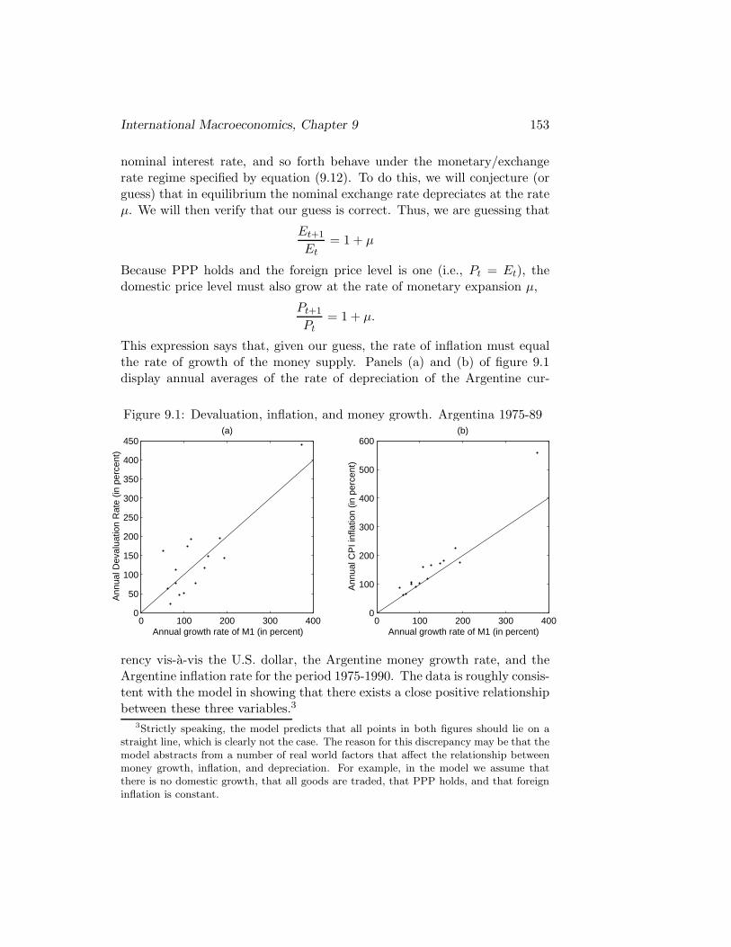
Figure 9.1: Devaluation, inflation, and money growth. Argentina 1975-89
0 100 200 300 4000
50
100
150
200
250
300
350
400
450
Annual growth rate of M1 (in percent)
Ann
ual D
eval
uatio
n R
ate
(in p
erce
nt)
(a)
0 100 200 300 4000
100
200
300
400
500
600
Annual growth rate of M1 (in percent)
Ann
ual C
PI i
nfla
tion
(in p
erce
nt)
(b)
rency vis-a-vis the U.S. dollar, the Argentine money growth rate, and theArgentine inflation rate for the period 1975-1990. The data is roughly consis-tent with the model in showing that there exists a close positive relationshipbetween these three variables.3
3Strictly speaking, the model predicts that all points in both figures should lie on astraight line, which is clearly not the case. The reason for this discrepancy may be that themodel abstracts from a number of real world factors that affect the relationship betweenmoney growth, inflation, and depreciation. For example, in the model we assume thatthere is no domestic growth, that all goods are traded, that PPP holds, and that foreigninflation is constant.
154 S. Schmitt-Grohe and M. Uribe
To determine the domestic nominal interest rate it, use the interest paritycondition (9.8)
1 + it = (1 + r∗)Et+1
Et= (1 + r∗)(1 + µ),
which implies that the nominal interest rate is constant and increasing inµ. When µ is positive, the domestic nominal interest rate exceeds the realinterest rate r∗ because the domestic currency is depreciating over time. Wesummarize the positive relationship between it and µ by writing
it = i(µ)
The notation i(µ) simply indicates that it is a function of µ. The func-tion i(µ) is increasing in µ. Substituting this expression into the liquiditypreference function (9.6) yields
Mt
Et= L(C, i(µ)). (9.13)
Note that C is a constant and that because the money growth rate µ isconstant, the nominal interest rate i(µ) is also constant. Therefore, the righthand side of (9.13) is constant. For the money market to be in equilibrium,the left-hand side of (9.13) must also be constant. This will be the case onlyif the exchange rate depreciates—grows—at the same rate as the moneysupply. This is indeed true under our initial conjecture that Et+1/Et =1 + µ. Equation (9.13) says that in equilibrium real money balances mustbe constant and that the higher the money growth rate µ the lower theequilibrium level of real balances.
Let’s now return to the government budget constraint (9.10), which wereproduce below for convenience
Bgt − Bg
t−1 =Mt − Mt−1
Et− DEFt
Let’s analyze the first term on the right-hand side of this expression, seignor-age revenue. Using the fact that Mt = EtL(C, i(µ)) (equation (9.13)), wecan write
Mt − Mt−1
Et=
EtL(C, i(µ)) − Et−1L(C, i(µ))Et
= L(C, i(µ))(
Et − Et−1
Et
)

International Macroeconomics, Chapter 9 155
Using the fact that the nominal exchange rate depreciates at the rate µ, thatis, Et = (1 + µ)Et−1, to eliminate Et and Et−1 from the above expression,we can write seignorage revenue as
Mt − Mt−1
Et= L(C, i(µ))
(µ
1 + µ
)(9.14)
Thus, seignorage revenue is equal to the product of real balances, L(C, i(µ)),and the factor µ/(1 + µ).
The right hand side of equation (9.14) can also be interpreted as theinflation tax. The idea is that inflation acts as a tax on the public’s holdingsof real money balances. To see this, let’s compute the change in the realvalue of money holdings from period t−1 to period t. In period t−1 nominalmoney holdings are Mt−1 which have a real value of Mt−1/Pt−1. In period tthe real value of Mt−1 is Mt−1/Pt. Therefore we have that the inflation taxequals Mt−1/Pt−1 − Mt−1/Pt, or, equivalently,
inflation tax =Mt−1
Pt−1
Pt − Pt−1
Pt
where Mt−1/Pt−1 is the tax base and (Pt − Pt−1)/Pt is the tax rate. Usingthe facts that in our model real balances are equal to L(C, i(µ)) and thatPt/Pt−1 = 1 + µ, the inflation tax can be written as
inflation tax = L(C, i(µ))µ
1 + µ,
which equals seignorage revenue. In general seignorage revenue and theinflation tax are not equal to each other. They are equal in the special casethat real balances are constant over time, like in our model when the moneysupply expands at a constant rate.
Because the tax base, real balances, is decreasing in µ and the tax rate,µ/(1+µ), is increasing in µ, it is not clear whether seignorage increases or de-creases with the rate of expansion of the money supply. Whether seignoragerevenue is increasing or decreasing in µ depends on the form of the liquiditypreference function L(·, ·) as well as on the level of µ itself. Typically, forlow values of µ seignorage revenue is increasing in µ. However, as µ getslarge the contraction in the tax base (the money demand) dominates theincrease in the tax rate and therefore seignorage revenue falls as µ increases.Thus, there exists a maximum level of revenue a government can collectfrom printing money. The resulting relationship between the growth rate ofthe money supply and seignorage revenue has the shape of an inverted-Uand is called the inflation tax Laffer curve (see figure 9.2).

156 S. Schmitt-Grohe and M. Uribe
Figure 9.2: The Laffer curve of inflation
0rate of growth of the money supply, µ
seig
nora
ge r
even
ue
Inflationary finance
We now use the theoretical framework developed thus far to analyze the linkbetween fiscal deficits, prices, and the exchange rate. Consider a situation inwhich the government is running constant fiscal deficits DEFt = DEF > 0for all t. Furthermore, assume that the government has reached its bor-rowing limit and thus cannot finance the fiscal deficits by issuing additionaldebt, so that Bg
t − Bgt−1 must be equal to zero. Under these circumstances,
the government budget constraint (9.10) becomes
DEF =Mt − Mt−1
Et
It is clear from this expression, that a country that has exhausted its abilityto issue public debt must resort to printing money in order to finance thefiscal deficit. This way of financing the public sector is called monetizationof the fiscal deficit. Combining the above expression with (9.14) we obtain
DEF = L(C, i(µ))(
µ
1 + µ
)(9.15)
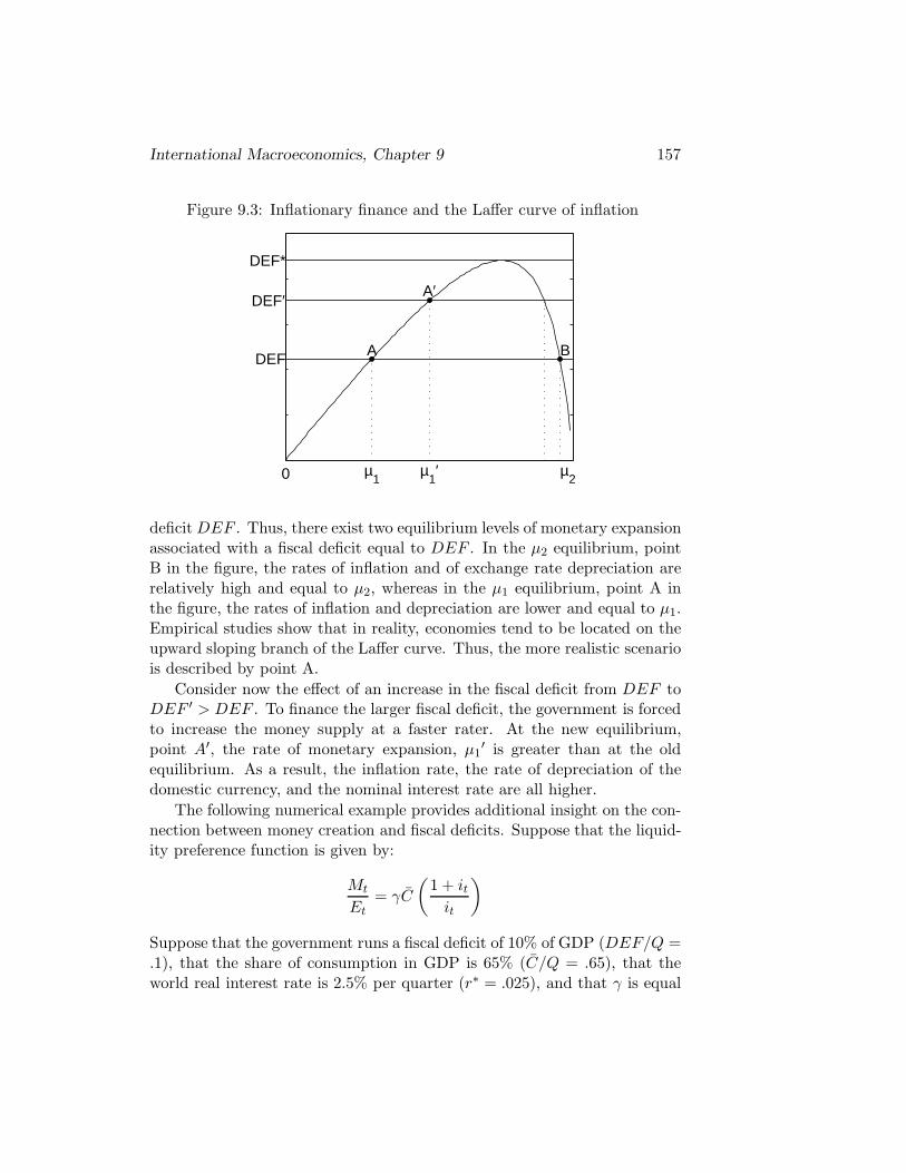
Figure 9.3 illustrates the relationship between fiscal deficits and the rate ofmonetary expansion implied by this equation. The Laffer curve of inflationcorresponds to the right hand side of (9.15). The horizontal line plots theleft hand side (9.15), or DEF . There are two rates of monetary expansion,µ1 and µ2, that generate enough seignorage revenue to finance the fiscal
International Macroeconomics, Chapter 9 157
Figure 9.3: Inflationary finance and the Laffer curve of inflation
0
A
µ1
B
µ2
DEF
DEF′
DEF*
A′
µ1′
deficit DEF . Thus, there exist two equilibrium levels of monetary expansionassociated with a fiscal deficit equal to DEF . In the µ2 equilibrium, pointB in the figure, the rates of inflation and of exchange rate depreciation arerelatively high and equal to µ2, whereas in the µ1 equilibrium, point A inthe figure, the rates of inflation and depreciation are lower and equal to µ1.Empirical studies show that in reality, economies tend to be located on theupward sloping branch of the Laffer curve. Thus, the more realistic scenariois described by point A.
Consider now the effect of an increase in the fiscal deficit from DEF toDEF ′ > DEF . To finance the larger fiscal deficit, the government is forcedto increase the money supply at a faster rater. At the new equilibrium,point A′, the rate of monetary expansion, µ1
′ is greater than at the oldequilibrium. As a result, the inflation rate, the rate of depreciation of thedomestic currency, and the nominal interest rate are all higher.
The following numerical example provides additional insight on the con-nection between money creation and fiscal deficits. Suppose that the liquid-ity preference function is given by:
Mt
Et= γC
(1 + it
it
)
Suppose that the government runs a fiscal deficit of 10% of GDP (DEF/Q =.1), that the share of consumption in GDP is 65% (C/Q = .65), that theworld real interest rate is 2.5% per quarter (r∗ = .025), and that γ is equal
158 S. Schmitt-Grohe and M. Uribe
to .16. The question is what is the rate of monetary expansion necessaryto monetize the fiscal deficit. Combining equations (9.2.6) and (9.15) andusing the fact 1 + it = (1 + r∗)(1 + µ) we have,
DEF = γC(1 + r∗)(1 + µ)
(1 + r∗)(1 + µ)− 1µ
1 + µ
Divide the left and right hand sides of this expression by Q and solve for µto obtain
µ =r∗(DEF/Q)
(1 + r∗)(γ(C/Q) − (DEF/Q))=
0.025 × 0.11.025 × (0.16 × 0.65 − 0.1)
= 0.61
The government must increase the money supply at a rate of 61% per quar-ter. This implies that both the rates of inflation and depreciation of thedomestic currency in this economy will be 61% per quarter. The nominalinterest rate is 65% per quarter. At a deficit of 10% of GDP, the Laffer curveis extremely flat. For example, if the government cuts the fiscal deficit by1% of GDP, the equilibrium money growth rate falls to 16%.
In some instances, inflationary finance can degenerate into hyperinfla-tion. Perhaps the best-known episode is the German hyperinflation of 1923.Between August 1922 and November 1923, Germany experienced an averagemonthly inflation rate of 322 percent.4 More recently, in the late 1980s anumber of hyperinflationary episodes took place in Latin America and East-ern Europe. One of the more severe cases was Argentina, where the inflationrate averaged 66 percent per month between May 1989 and March 1990.
A hyperinflationary situation arises when the fiscal deficit reaches a levelthat can no longer be financed by seignorage revenue alone. In terms offigure 9.3, this would be the case if the fiscal deficit would be larger thanDEF ∗, the level of deficit associated with the peak of the Laffer curve. Whathappens in practice is that the government is initially unaware of the factthat no rate of monetary expansion will suffice to finance the deficit. In itsattempt to close the fiscal gap, the government accelerates the rate of moneycreation. But this measure is counterproductive because the governmenthas entered the downward sloping side of the Laffer curve. The decline inseignorage revenue leads the government to increase the money supply atan even faster rate. These dynamics turn into a vicious cycle that ends inan accelerating inflationary spiral. The most fundamental step in ending
4A fascinating account of four Post World War I European hyperinflations is given inSargent, “The End of Four Big Inflations,” in Robert Hall, editor, Inflation: Causes andEffects, The University of Chicago Press, Chicago, 1982.
International Macroeconomics, Chapter 9 159
hyperinflation is to eliminate the underlying budgetary imbalances that areat the root of the problem. When this type of structural fiscal reforms isundertaken and is understood by the public, hyperinflation typically stopsabruptly.
Money growth and inflation in a growing economy
Thus far, we have considered the case in which consumption is constant overtime.5 We now wish to consider the case that consumption is growing overtime. Specifically, we will assume that consumption grows at a constant rateγ > 0, that is,
Ct+1 = (1 + γ)Ct.
We also assume that the liquidity preference function is of the form
L(Ct, it) = Ctl(it)
where l(·) is a decreasing function.6 Consider again the case that the gov-ernment expands the money supply at a constant rate µ > 0. As before, wefind the equilibrium by first guessing the value of the depreciation rate andthen verifying that this guess indeed can be supported as an equilibriumoutcome. Specifically, we conjecture that the domestic currency depreciatesat the rate (1 + µ)/(1 + γ) − 1, that is,
Et+1
Et=
1 + µ
1 + γ
Our conjecture says that given the rate of monetary expansion, the higherthe rate of economic growth, the lower the rate of depreciation of the domes-tic currency. In particular, if the government wishes to keep the domesticcurrency from depreciating, it can do so by setting the rate of monetary ex-pansion at a level no greater than the rate of growth of consumption (µ ≤ γ).By interest rate parity,
(1 + it) = (1 + r∗)Et+1
Et
= (1 + r∗)(1 + µ)(1 + γ)
5Those familiar with the appendix will recognize that the constancy of consumptionis a direct implication of our assumption that the subjective discount rate is equal to theworld interest rate, that is, β(1 + r∗) = 1. It is clear from (9.19) that consumption willgrow over time only if β(1 + r∗) is greater than 1.
6Can you show that this form of the liquidity preference function obtains when theperiod utility function is given by lnCt + θ ln(Mt/Et). Under this particular preferencespecification find the growth rate of consumption γ as a function of β and 1 + r∗.

160 S. Schmitt-Grohe and M. Uribe
This expression says that the nominal interest rate is constant over time.We can summarize this relationship by writing
it = i(µ, γ), for all t
where the function i(µ, γ) is increasing in µ and decreasing in γ. Equilibriumin the money market requires that the real money supply be equal to thedemand for real balances, that is,
Mt
Et= Ctl(i(µ, γ))
The right-hand side of this expression is proportional to consumption, andtherefore grows at the gross rate 1+ γ. The numerator of the left hand sidegrows at the gross rate 1 + µ. Therefore, in equilibrium the denominator ofthe left hand side must expand at the gross rate (1 + µ)/(1 + γ), which isprecisely our conjecture.
Finally, by PPP and given our assumption that P ∗t = 1, we have that
the domestic price level, Pt, must be equal to the nominal exchange rate,Et. It follows that the domestic rate of inflation must be equal to the rateof depreciation of the nominal exchange rate, that is,
Pt − Pt−1
Pt−1=
Et − Et−1
Et−1=
1 + µ
1 + γ− 1
This expression shows that to the extend that consumption growth is pos-itive the domestic inflation rate is lower than the rate of monetary expan-sion. The intuition for this result is straightforward. A given increase inthe money supply that is not accompanied by an increase in the demand forreal balances will translate into a proportional increase in prices. This is be-cause in trying to get rid of their excess nominal money holdings householdsattempt to buy more goods. But since the supply of goods is unchangedthe increased demand for goods will be met by an increase in prices. Thisis a typical case of ”more money chasing the same amount of goods.” Whenthe economy is growing, the demand for real balances is also growing. Thatmeans that part of the increase in the money supply will not end up chasinggoods but rather will end up in the pockets of consumers.
9.3 Balance-of-payments crises
A balance of payments, or BOP, crisis is a situation in which the governmentis unable or unwilling to meet its financial obligations. These difficulties may
International Macroeconomics, Chapter 9 161
manifest themselves in a variety of ways, such as the failure to honor thedomestic and/or foreign public debt or the suspension of currency convert-ibility.
What causes BOP crises? Sometimes a BOP crisis arises as the in-evitable consequence of unsustainable combinations of monetary and fiscalpolicies. A classic example of such a policy mix is a situation in which agovernment pegs the nominal exchange rate and at the same time runs afiscal deficit. As we discussed in subsection 9.2.5, under a fixed exchangerate regime, the government must finance any fiscal deficit by running downits stock of interest bearing assets (see equation (9.11)). Clearly, to theextent that there is a limit to the amount of debt a government is able toissue, this situation cannot continue indefinitely. When the public debt hitsits upper limit the government is forced to change policy. One possibility isthat the government stops servicing the debt (i.e., stops paying interest onits outstanding financial obligations), thereby reducing the size of the sec-ondary deficit. This alternative was adopted by Mexico in August of 1982,when it announced that it would be unable to honor its debt commitmentsaccording to schedule, marking the beginning of what today is known as theDeveloping Country Debt Crisis. A second possibility is that the govern-ment adopt a fiscal adjustment program by cutting government spendingand raising regular taxes and in that way reduce the primary deficit. Fi-nally, the government can abandon the exchange rate peg and resort tomonetizing the fiscal deficit. This has been the fate of the vast majorityof currency pegs adopted in developing countries. The economic history ofLatin America of the past two decades is plagued with such episodes. Forexample, the currency pegs implemented in Argentina, Chile, and Uruguayin the late 1970s, also known as tablitas, ended with large devaluations inthe early 1980s; similar outcomes were observed in the Argentine Australstabilization plan of 1985, the Brazilian Cruzado plan of 1986, the Mexicanplan of 1987, and, more recently the Brazilian Real plan of 1994.
An empirical regularity associated with the collapse of fixed exchangerate regimes is that in the days immediately before the peg is abandoned, thecentral bank looses vast amounts of reserves in a short period of time. Theloss of reserves is the consequence of a run by the public against the domesticcurrency in anticipation of the impending devaluation. The stampede ofpeople trying to massively get rid of domestic currency in exchange forforeign currency is driven by the desire to avoid the loss of real value ofdomestic currency denominated assets that will take place when the currencyis devalued.
The first formal model of the dynamics of a fixed exchange rate collapse

162 S. Schmitt-Grohe and M. Uribe
is due to Paul R. Krugman of Princeton University.7 In this section, we willanalyze these dynamics using the tools developed in sections 9.2.5 and 9.2.6.These tools will helpful in a natural way because, from an analytical pointof view, the collapse of a currency peg is indeed a transition from a fixed toa floating exchange rate regime.
Consider a country that is running a constant fiscal deficit DEF > 0each period. Suppose that in period 1 the country embarks in a currencypeg. Specifically, assume that the government fixes the nominal exchangerate at E units of domestic currency per unit of foreign currency. Supposethat in period 1, when the currency peg is announced, the government has apositive stock of foreign assets carried over from period 0, Bg
0 > 0. Further,assume that the government does not have access to credit. That is, thegovernment asset holdings are constrained to being nonnegative, or Bg
t ≥ 0for all t. It is clear from our discussion of the sustainability of currency pegsin subsection 9.2.5 that, as long as the currency peg is in effect, the fiscaldeficit produces a continuous drain of assets, which at some point will becompletely depleted. Put differently, if the fiscal deficit is not eliminated,at some point the government will be forced to abandon the currency pegand start printing money in order to finance the deficit. Let T denote theperiod in which, as a result of having run out of reserves, the governmentabandons the peg and begins to monetize the fiscal deficit.
The dynamics of the currency crisis are characterized by three distinctphases. (1) The pre-collapse phase: during this phase, which lasts from t = 1to t = T −2, the currency peg is in effect. (2) The BOP crisis: It takes placein period t = T − 1, and is the period in which the central bank faces a runagainst the domestic currency, resulting in massive losses of foreign reserves.(3) The post-collapse phase: It encompasses the period from t = T onwardsIn this phase, the nominal exchange rate floats freely and the central bankexpands the money supply at a rate consistent with the monetization of thefiscal deficit.
(1) The pre-crisis phase: from t = 1 to t = T − 2
From period 1 to period T − 2, the exchange rate is pegged, so the variablesof interest behave as described in section 9.2.5. In particular, the nominalexchange rate is constant and equal to E, that is, Et = E for t = 1, 2, . . . , T−2. By PPP, and given our assumption that P ∗
t = 1, the domestic price levelis also constant over time and equal to E (Pt = E for t = 1, 2, . . . , T − 2).
7The model appeared in Paul R. Krugman, “A Model of Balance-of-Payments Crisis,”Journal of Money, Credit and Banking, 11, 1979, 311-325.
International Macroeconomics, Chapter 9 163
Because the exchange rate is fixed, the devaluation rate (Et−Et−1)/Et−1, isequal to 0. The nominal interest, it, which by the uncovered interest paritycondition satisfies 1 + it = (1 + r∗)Et+1/Et, is equal to r∗. Note that thenominal interest rate in period T −2 is also equal to r∗ because the exchangerate peg is still in place in period T −1. Thus, it = r∗ for t = 1, 2, . . . , T −2.
As discussed in section 9.2.5, by pegging the exchange rate the govern-ment relinquishes its ability to monetize the deficit. This is because thenominal money supply, Mt, which in equilibrium equals EL(C, r∗), is con-stant, and as a result seignorage revenue, given by (Mt − Mt−1)/E, is nil.Consider now the dynamics of foreign reserves. By equation (9.11),
Bgt − Bg
t−1 = −DEF ; for t = 1, 2, . . . , T − 2.
This expression shows that the fiscal deficit causes the central bank to loseDEF units of foreign reserves per period. The continuous loss of reservesin combination with the lower bound on the central bank’s assets, makes itclear that a currency peg is unsustainable in the presence of persistent fiscalimbalances.
(3) The post-crisis phase: from t = T onwards
The government starts period T without any foreign reserves (BgT−1 = 0).
Given our assumptions that the government cannot borrow (that is, Bgt
cannot be negative) and that it is unable to eliminate the fiscal deficit,it follows that in period T the monetary authority is forced to abandonthe currency peg and to print money in order to finance the fiscal deficit.Thus, in the post-crisis phase the government lets the exchange rate float.Consequently, the behavior of all variables of interest is identical to thatstudied in subsection 9.2.6. In particular, the government will expand themoney supply at a constant rate µ that generates enough seignorage revenueto finance the fiscal deficit. In section 9.2.6, we deduced that µ is determinedby equation (9.15),
DEF = L(C, i(µ))(
µ
1 + µ
)
Note that because the fiscal deficit is positive, the money growth rate mustalso be positive. In the post-crisis phase, real balances, Mt/Et are constantand equal to L(C, i(µ)). Therefore, the nominal exchange rate, Et, mustdepreciate at the rate µ. Because in our model Pt = Et, the price level alsogrows at the rate µ, that is, the inflation rate is positive and equal to µ.
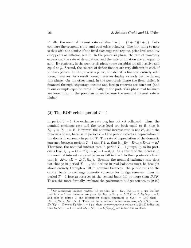
164 S. Schmitt-Grohe and M. Uribe
Finally, the nominal interest rate satisfies 1 + it = (1 + r∗)(1 + µ). Let’scompare the economy’s pre- and post-crisis behavior. The first thing to noteis that with the demise of the fixed exchange rate regime, price level stabilitydisappears as inflation sets in. In the pre-crisis phase, the rate of monetaryexpansion, the rate of devaluation, and the rate of inflation are all equal tozero. By contrast, in the post-crisis phase these variables are all positive andequal to µ. Second, the sources of deficit finance are very different in each ofthe two phases. In the pre-crisis phase, the deficit is financed entirely withforeign reserves. As a result, foreign reserves display a steady decline duringthis phase. On the other hand, in the post-crisis phase the fiscal deficit isfinanced through seignorage income and foreign reserves are constant (andin our example equal to zero). Finally, in the post-crisis phase real balancesare lower than in the pre-crisis phase because the nominal interest rate ishigher.
(2) The BOP crisis: period T − 1
In period T − 1, the exchange rate peg has not yet collapsed. Thus, thenominal exchange rate and the price level are both equal to E, that isET−1 = PT−1 = E. However, the nominal interest rate is not r∗, as in thepre-crisis phase, because in period T −1 the public expects a depreciation ofthe domestic currency in period T . The rate of depreciation of the domesticcurrency between periods T −1 and T is µ, that is, (ET −ET−1)/ET−1 = µ.8
Therefore, the nominal interest rate in period T − 1 jumps up to its post-crisis level iT−1 = (1 + r∗)(1 + µ) − 1 = i(µ). As a result of the increase inthe nominal interest rate real balances fall in T − 1 to their post-crisis level,that is, MT−1/E = L(C, i(µ)). Because the nominal exchange rate doesnot change in period T − 1, the decline in real balances must be broughtabout entirely through a fall in nominal balances: the public runs to thecentral bank to exchange domestic currency for foreign reserves. Thus, inperiod T − 1 foreign reserves at the central bank fall by more than DEF .To see this more formally, evaluate the government budget constraint (9.10)
8For technically inclined readers: To see that (ET − ET−1)/ET−1 = µ, use the factthat in T − 1 real balances are given by MT−1/ET−1 = L(C, (1 + r∗)ET /ET−1 − 1)and that in period T the government budget constraint is DEF = L(C, i(µ)) −(MT−1/ET−1)(ET−1/ET ). These are two equations in two unknowns, MT−1/ET−1 andET /ET−1. If we set ET /ET−1 = 1+µ, then the two equations collapse to (9.15) indicatingthat ET /ET−1 = 1 + µ and MT−1/ET−1 = L(C, i(µ)) are indeed the solution.
International Macroeconomics, Chapter 9 165
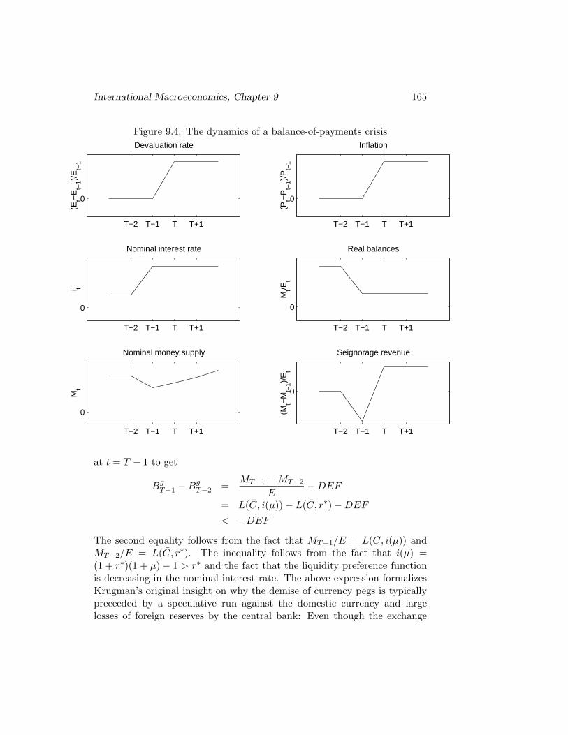
Figure 9.4: The dynamics of a balance-of-payments crisis
T−2 T−1 T T+1
0
(Et−
Et−
1)/E
t−1
Devaluation rate
T−2 T−1 T T+1
0
(Pt−
Pt−
1)/P
t−1
Inflation
T−2 T−1 T T+1
0
Nominal interest rate
i t
T−2 T−1 T T+1
0
Real balances
Mt/E
t
T−2 T−1 T T+1
0
Nominal money supply
Mt
T−2 T−1 T T+1
0
Seignorage revenue
(Mt−
Mt−
1)/E
t
at t = T − 1 to get
BgT−1 − Bg
T−2 =MT−1 − MT−2
E− DEF
= L(C, i(µ)) − L(C, r∗)− DEF
< −DEF
The second equality follows from the fact that MT−1/E = L(C, i(µ)) andMT−2/E = L(C, r∗). The inequality follows from the fact that i(µ) =(1 + r∗)(1 + µ) − 1 > r∗ and the fact that the liquidity preference functionis decreasing in the nominal interest rate. The above expression formalizesKrugman’s original insight on why the demise of currency pegs is typicallypreceeded by a speculative run against the domestic currency and largelosses of foreign reserves by the central bank: Even though the exchange

166 S. Schmitt-Grohe and M. Uribe
rate is pegged in T − 1, the nominal interest rate rises in anticipation ofa devaluation in period T causing a contraction in the demand for realmoney balances. Because in period T − 1 the domestic currency is stillfully convertible, the central bank must absorb the entire decline in thedemand for money by selling foreign reserves. Figure 9.4 closes this sectionby providing a graphical summary of the dynamics of Krugman-type BOPcrises.
9.4 Appendix: A dynamic optimizing model ofthe demand for money
In this section we develop a dynamic optimizing model underlying the liq-uidity preference function given in equation (9.6). We motivate a demandmoney by assuming that money facilitates transactions. We capture the factthat money facilitates transactions by simply assuming that agents deriveutility not only from consumption of goods but also from holdings of realbalances. Specifically, in each period t = 1, 2, 3, . . . preferences are describedby the following single-period utility function,
u(Ct) + z
(Mt
Pt
),
where Ct denotes the household’s consumption in period t and Mt/Pt de-notes the household’s real money holdings in period t. The functions u(·)and z(·) are strictly increasing and strictly concave functions (u′ > 0, z′ > 0,u′′ < 0, z′′ < 0).
Households are assumed to be infinitely lived and to care about theirentire stream of single-period utilities. However, households discount thefuture by assigning a greater weight to consumption and real money holdingsthe closer they are to the present. Specifically, their lifetime utility functionis given by[u(Ct) + z
(Mt
Pt
)]+ β
[u(Ct+1) + z
(Mt+1
Pt+1
)]+ β2
[u(Ct+2) + z
(Mt+2
Pt+2
)]+ . . .
Here β is a number greater than zero and less than one called the subjectivediscount factor.” The fact that households care more about the present thanabout the future is reflected in β being less than one.
Let’s now analyze the budget constraint of the household. In period t,the household allocates its wealth to purchase consumption goods, PtCt, to

International Macroeconomics, Chapter 9 167
hold money balances, Mt, to pay taxes, Tt, and to purchase interest bearingforeign bonds, EtB
pt . Taxes are lump sum and denominated in domestic
currency. The foreign bond is denominated in foreign currency. Each unitof foreign bonds costs 1 unit of the foreign currency, so each unit of theforeign bond costs Et units of domestic currency. Foreign bonds pay theconstant world interest rate r∗ in foreign currency. Note that because theforeign price level is assumed to be constant, r∗ is not only the interest ratein terms of foreign currency but also the interest rate in terms of goods.That is, r∗ is the real interest rate.9 The superscript p in Bp
t , indicatesthat these are bond holdings of private households, to distinguish themfrom the bond holdings of the government, which we will introduce later.In turn, the household’s wealth at the beginning of period t is given bythe sum of its money holdings carried over from the previous period, Mt−1,bonds purchased in the previous period plus interest, Et(1 + r∗)Bp
t−1, andincome from the sale of its endowment of goods, PtQt, where Qt denotes thehousehold’s endowment of goods in period t. This endowment is assumedto be exogenous, that is, determined outside of the model. The budgetconstraint of the household in period t is then given by:
PtCt + Mt + Tt + EtBpt = Mt−1 + (1 + r∗)EtB
pt−1 + PtQt (9.16)
The left hand side of the budget constraint represents the uses of wealthand the right hand side the sources of wealth. The budget constraint isexpressed in nominal terms, that is, in terms of units of domestic currency.To express the budget constraint in real terms, that is, in units of goods, wedivide both the left and right hand sides of (9.16) by Pt, which yields
Ct +Mt
Pt+
Tt
Pt+
Et
PtBp
t =Mt−1
Pt−1
Pt−1
Pt+ (1 + r∗)
Et
PtBp
t−1 + Qt
Note that real balances carried over from period t − 1, Mt−1/Pt−1, appearmultiplied by Pt−1/Pt. In an inflationary environment, Pt is greater thanPt−1, so inflation erodes a fraction of the household’s real balances. This lossof resources due to inflation is called the inflation tax. The higher the rateof inflation, the larger the fraction of their income households must allocateto maintaining a certain level of real balances.
Recalling that Pt equals Et, we can eliminate Pt from the utility function
9The domestic nominal and real interest rates will in general not be equal to each otherunless domestic inflation is zero. To see this, recall the Fisher equation (5.3). We willreturn to this point shortly.

168 S. Schmitt-Grohe and M. Uribe
and the budget constraint to obtain:[u(Ct) + z
(Mt
Et
)]+ β
[u(Ct+1) + z
(Mt+1
Et+1
)]+ β2
[u(Ct+2) + z
(Mt+2
Et+2
)]+ . . .
(9.17)
Ct +Mt
Et+
Tt
Et+ Bp
t =Mt−1
Et+ (1 + r∗)Bp
t−1 + Qt (9.18)
Households choose Ct, Mt, and Bpt so as to maximize the utility function
(9.17) subject to a series of budget constraints like (9.18), one for each pe-riod, taking as given the time paths of Et, Tt, and Qt. In choosing streams ofconsumption, money balances, and bonds, the households faces two trade-offs. The first tradeoff is between consuming today and saving today tofinance future consumption. The second tradeoff is between consuming to-day and holding money today.
Consider first the tradeoff between consuming one extra unit of the goodtoday and investing it in international bonds to consume the proceeds to-morrow. If the household chooses to consume the extra unit of goods today,then its utility increases by u′(Ct). Alternatively, the household could sellthe unit of good for 1 unit of foreign currency and with the proceeds buy1 unit of the foreign bond. In period t + 1, the bond pays 1 + r∗ units offoreign currency, with which the household can buy (1 + r∗) units of goods.This amount of goods increases utility in period t + 1 by (1 + r∗)u′(Ct+1).Because households discount future utility at the rate β, from the point ofview of period t, lifetime utility increases by β(1 + r∗)u′(Ct+1). If the firstalternative yields more utility than the second, the household will increaseconsumption in period t, and lower consumption in period t + 1. This willtend to eliminate the difference between the two alternatives because it willlower u′(Ct) and increase u′(Ct+1) (recall that u(·) is concave, so that u′(·) isdecreasing). On the other hand, if the second alternative yields more utilitythan the first, the household will increase consumption in period t + 1 anddecrease consumption in period t. An optimum occurs at a point wherethe household cannot increase utility further by shifting consumption acrosstime, that is, at an optimum the household is, in the margin, indifferent be-tween consuming an extra unit of good today or saving it and consuming theproceeds the next period. Formally, the optimal allocation of consumptionacross time satisfies
u′(Ct) = β(1 + r∗)u′(Ct+1) (9.19)
International Macroeconomics, Chapter 9 169
We will assume for simplicity that the subjective rate of discount equalsthe world interest rate, that is,
β(1 + r∗) = 1 (9.20)
Combining this equation with the optimality condition (9.19) yields,
u′(Ct) = u′(Ct+1) (9.21)
Because u(·) is strictly concave, u′(·) is monotonically decreasing, so thisexpressions implies that Ct = Ct+1. This relationship must hold in allperiods, implying that consumption is constant over time. Let C be thisoptimal level of consumption. Then, we have
Ct = Ct+1 = Ct+2 = · · · = C
Consider now the tradeoff between spending one unit of money on con-sumption and holding it for one period. If the household chooses to spendthe unit of money on consumption, it can purchase 1/Et units of goods,which yield u′(Ct)/Et units of utility. If instead the household chooses tokeep the unit of money for one period, then its utility in period t increasesby z′(Mt/Et)/Et. In period t + 1, the household can use the unit of moneyto purchase 1/Et+1 units of goods, which provide u′(Ct+1)/Et+1 extra utils.Thus, the alternative of keeping the unit of money for one period yieldsz′(Mt/Et)/Et + βu′(Ct+1)/Et+1 additional units of utility. In an optimum,the household must be indifferent between keeping the extra unit of moneyfor one period and spending it on current consumption, that is,
z′(Mt/Et)Et
+ βu′(Ct+1)
Et+1=
u′(Ct)Et
(9.22)
Using the facts that u′(Ct) = u′(Ct+1) = u′(C) and that β = 1/(1+ r∗) andrearranging terms we have
z′(
Mt
Et
)= u′(C)
[1 − Et
(1 + r∗)Et+1
](9.23)
Using the uncovered interest parity condition (9.8) we can write
z′(
Mt
Et
)= u′(C)
(it
1 + it
)(9.24)
This equation relates the demand for real money balances, Mt/Et, to thelevel of consumption and the domestic nominal interest rate. Inspecting
170 S. Schmitt-Grohe and M. Uribe
equation (9.24) and recalling that both u and z are strictly concave, revealsthat the demand for real balances, Mt/Et, is decreasing in the level of thenominal interest rate, it, and increasing in consumption, C. This relation-ship is called the liquidity preference function. We write it in a compactform as
Mt
Et= L(C, it)
which is precisely equation (9.6).The following example derives the liquidity preference function for a
particular functional form of the period utility function. Assume that
u(Ct) + z(Mt/Et) = lnCt + γ ln(Mt/Et).
Then we have u′(C) = 1/C and z′(Mt/Et) = γ/(Mt/Et). Therefore, equa-tion (9.24) becomes
γ
Mt/Et=
1C
(it
1 + it
)
The liquidity preference function can be found by solving this expression forMt/Et. The resulting expression is in fact the liquidity preference functiongiven in equation (9.2.6), which we reproduce here for convenience.
Mt
Et= γC
(it
1 + it
)−1
In this expression, Mt/Et is linear and increasing in consumption and de-creasing in it.