MONETARY POLICY AND EXCHANGE RATEARRANGEMENTS IN EAST ASIA BEFORE AND AFTER

THE CRISIS.

Tony Cavoli

Thesis submitted to the School of Economics, University of Adelaide for Fulfilmentof the Degree of Doctor of Philosophy.

February,2005

by

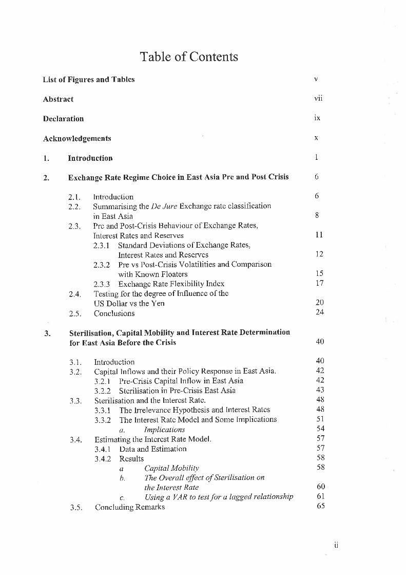
Table of Contents

List of Figures and Tables

Abstract

Declaration

Acknowledgements

1. Introduction

2. Exchange Rate Regime Choice in East Asia Pre and Post Crisis

V

v11

ix

X

1

2.t.2.2.

L.)

2.5

3.1.3.2.

J.J

IntroductionSummarising the De Jure Exchange rate classificationin East AsiaPre and Post-Crisis Behaviour of Exchange Rates,Interest Rates and Reserves2.3.7 Standard Deviations of Exchange Rates,

lnterest Rates and Reserves2.3.2 Pre vs Post-Crisis Volatilities and Comparison

with Known Floaters2.3.3 Exchange Rate Flexibility IndexTesting for the degree of Influence of theUS Dollar vs the YenConclusions

IntroductionCapital Inflows and their Policy Response in East Asia'3.2.1 Pre-Crisis Capital Inflow in East Asia3.2.2 Sterilisation in Pre-Crisis East AsiaSterilisation and the Interest Rate.3.3.1 The htelevance Hlpothesis and Interest Rates3.3.2 The Interest Rate Model and Some Implications

a. ImplicationsEstimating the Interest Rate Model.3.4.1 Data and Estimation3.4.2 Results

a Capital Mobilityb. The Overall effect of Sterilisation on

the Interest Ratec. Using a VAR to test for a lagged relationship

Concluding Remarks

6

6

8

11

12

2.4.

15

T7

4042

4348485154575l5858

606l65

2024

403. Sterilisation, Capital Mobility and Interest Rate Determination

for East Asia Before the Crisis

42

3.4.

3.5

ll

4 Inflation Targeting and Monetary Policy Rules in East AsiaPost Crisis: With Particular Reference to Thailand 76

76788284878788899T91949597100

1115.

4.t.4.2.4.3.

4.4.

4.5

IntroductionInflation Targeting in East AsiaOpen Economy Inflation Targeting4.3.1 Small Open Economy Macro Model4.3.2 Simple vs Optimal Monetary Policy Rules (MPRs)

a. Simple MPRsb. Optimal MPRsc. Comparisons

Model Parameterisation, Empirical Analysis and Results4.4.I Model parameterisation4.4.2 Stochastic and Dynamic Results

a. Unconditional Standard Deviationsb. Impulse Response Functions

Conclusions

IntroductionReasons for Fear of Floating5.2.1. Trade Pattems and Trade Openness5.2.2. Exchange Rate Passthrough5.2.3. Balance Sheet EffectsModel and Solution5.3.1 Small Open macro Model5.3.2 Fear of floating Scenarios and Monetary Policy

OptionsResults5.4.I Coefficients to the Optimal lnterest rate Rules5.4.2 Stochastic properties5.4.3 Dynamic PropertiesConclusions

Fear of Floating and optimal Monetary Policy: With ParticularReference to East Asia

5.1.5.2.

111Ir4tt4115I17t20120

t24t26r26t28130r33

743

t49

149

149

5.3

5.4

5.5

6. Conclusions, Policy implications and Scope forFurther Research

Appendix 1. Appendix to Chapter 3

14. Augmented Dickey-Fuller (ADF) Tests for Money Market Rates

18. ADF Tests for Regression Residuals for Korea and Malaysia

Appendix 2. Appendix to Chapter 4 150

lll

2A.

Appendix 3. Appendix to Chapter 4 and Chapter 5

34. State Space Representation of Model in Chapter 5

38.

References

Solution for unique Rational Expectations equilibrium in alinear, dynamic, stochastic macroeconomic model.

- Optimal monetary policy under commitment- Simple, fixed monetary policy rule

Solution for unique Rational Expectations equilibrium in alinear, dynamic, stochastic macroeconomic model.

- Optimal monetary policy under discretion

150ts4

1s6

156

r57

161

1V

FIGURES

List of Figures and Tables

Exchange Rates, 1990-2004

Standard Deviations, Exchange Rates/US Dollar

Standard Deviations, Exchange Rates/Yen

Standard Deviations, REER

Standard Deviations, Interest Rates

Standard Deviations, Reserves/Lagged Money Base

Flexibility Index #1

Flexibility Index#2

Flexibility Index #3

Kalman Filter Results

Kalman Filter Results

Reserve Sterilisation

Rolling Regressions - Sterilisation

Interest Rates, 1990-1997

Variance Decomposition of i

Diagrammatic Representation of Thailand' s Monetary

Policy Transmission

Inflation Rates

Output/Infl ation volatility Tradeoffs

Impulse Responses

Impulse Responses

Impulse Responses, Baseline Model

Impulse Responses, High Openness

Impulse Responses, Delayed Pass-through

Impulse Responses, Financial Vulnerability

De Jure Exchange Rate Classifications

Standard Deviations Pre and Post-Crisis

OLS Estimates using Frankel and Wei (1994) Methodology

Figure 2.1:

Figure 2.2a:

Figure2.2b:

Figure2.2c:

Figure 2.3:

Figure2.4:

Figure 2.5a:

Figure 2.5b:

Figure 2.5c:

Figure 2.6:

Figure 2.7:

Figure 3.1:

Figure 3.2:

Figure 3.3:

Figure 3.4:

Figure 4.1:

29

30

31

32

JJ

34

35

36

37

38

39

70

/5

74

75

Figure 4.2:

Figure 4.3:

Figure 4.4-5:

Figure 4.6-7:

Figure 5.1 :

Figure 5.2:

Figure 5.3:

Figure 5.4:

107

108

108

109

110

t39

140

t4tr42

27

27

28

TABLES

Table2.l:

Table 2.2:

Table 2.3:

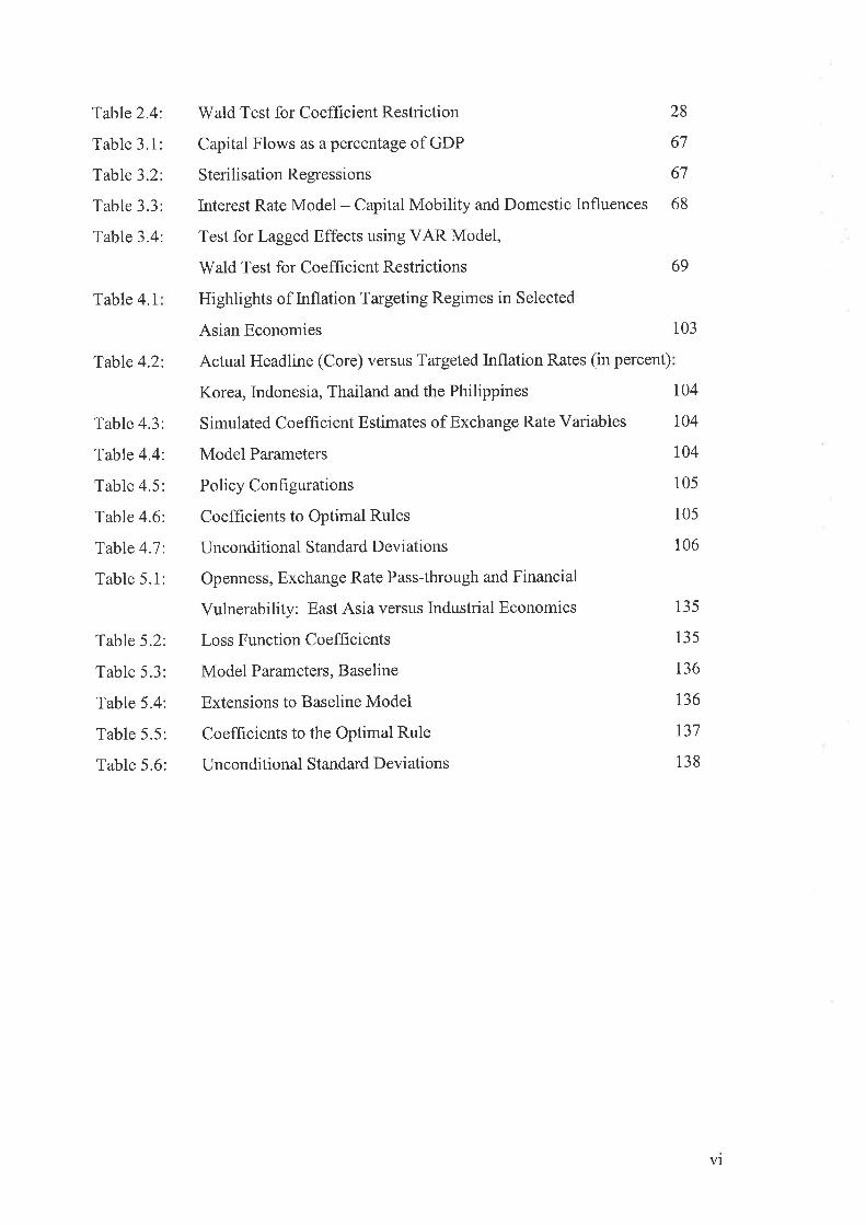
Table2.4:

Table 3.1:

Table 3.2:

Table 3.3:

Table 3.4:

Table 4.1

Table 4.2:

Table 4.3:

Table 4.4:

Table 4.5:

Table 4.6:

Table 4.7:

Table 5.1:

Table 5.2:

Table 5.3:

Table 5.4:

Table 5.5:

Table 5.6:

Wald Test for Coefficient Restriction

Capital Flows as a percentage of GDP

Sterilisation Regressions

lnterest Rate Model - Capital Mobility and Domestic Influences

Test for Lagged Effects using VAR Model,

Wald Test for Coefnicient Restrictions

Highlights of Inflation Targeting Regimes in Selected

Asian Economies

Actual Headline (Core) versus Targeted Inflation Rates (in percent)

Korea, Indonesia, Thailand and the Philippines

Simulated Coefficient Estimates of Exchange Rate Variables

Model Parameters

Policy Configurations

Coefficients to Optimal Rules

Unconditional Standard Deviations

Openness, Exchange Rate Pass-through and Financial

Vulnerability: East Asia versus Industrial Economies

Loss Function Coefficients

Model Parameters, Baseline

Extensions to Baseline Model

Coefficients to the Optimal Rule

Unconditional Standard Deviations

28

67

67

68

t04

104

t04

105

105

106

69

103

135

13s

t36

136

t37

138

v1

MONETARY POLICY AND EXCHANGE RATE ARRAI{GEMENTSIN EAST ASIA BEFORE AND AF'TER THE CRISIS.

AbstractThis dissertation examines the monetary policy and exchange rate regime choices

made by central banks in East Asia before and after the Asian Crisis in 1997-8. The

crisis was something of a defining moment in the way central banks conducted their

monetary policy and all of the crisis-affected economies - Korea, Thailand, Indonesia,

Malaysia and the Philippines substantially changed their policies thereafter.l Chapter 2

offers an empirical overview and analysis of the monetary policy and exchange rate

arrangements before and after the crisis.

Before the crisis, each of the countries mentioned above conducted largely

exchange rate based monetary policy that centred around a soft US dollar peg (although

Philippines was more of a chaotic managed float). Reserves were used to manipulate the

value of the local currency against the US dollar and, as such, the central banks of these

countries subordinated much of their monetary policy, and therefore interest rate

movements, to the US. Any attempt at establishing monetary control was with the aid of

sterilised intervention. As such Chapter 3 of this dissertation presents a model assessing

the effectiveness of sterilised intervention and the effect of sterilisation on domestic

interest rates. The results indicate significant evidence of sterilisation before the crisis

in all the countries sampled. Furthermore, the existence of sterilisation had a weak

impact on the domestic interest rate for Korea, Thailand, the Philippines and Malaysia,

but a stronger effect in lndonesia. When the model is generalised to incorporate alag

structure using a VAR, the effects are stronger across the board'

' Singapore and Taiwan were also affected. Data for Taiwan is diffrcult to obtain and Singapore's regimeis rather unusual and didn't lend itselfto the type analysis conducted in this dissertation.

vll

After the crisis, Malaysia (Spetember 1998) instituted a system of rigidly fixed

exchange rates and effective capital controls. Korea, Thailand, Indonesia and the

Philippines instituted an inflation-targeting (IT) regime fashioned around a floating

exchange rate, Chapter 4 focuses on the effectiveness of IT regimes in East Asia. A

simple analytical model is specified and calibrated using data for Thailand. The model

is then simulated to examine arange of different policypositions; and the stochastic and

dynamic properties of the model are generated and analysed. The results show that IT is

more effective when the exchange rate is included as part of the central bank's set of

objectives. An important feature of the parameterisation of the model is the existence of

possible contractionary devaluation, which further promotes the uses of exchange rate

augmented IT based policies.

One of the main results from the study in Chapter 2 is that, while there was a

general increase in the flexibility of exchange rates, they did not float as freely as they do

in countries like Australia and the USA - countries known to be 'floaters'. There seems

to be a fear of floating (FoF) in many cases. Chapter 5 analyses the existence of, and

possible justification for, FoF and examines the effectiveness of different optimal

monetary policy types using a small open-economy model and dynamic programming

techniques. The policies examined are solved in the model as optimal policy under

discretion. The numerical results indicate that, for most model configurations, those

polices with exchange rate involvement perform well and in some cases are the most

suited policy. This suggests that there may be some justification for fear of floating

attitudes amongst central banks. FoF policies appear to control exchange rate

movements with relatively little cost to inflation for most scenarios examined.

Chapter 6 offers some concluding remarks and discusses the scope for future

research on this topic.

v111

Declaration

This work contains no material which has been accepted for the award of any

other degree or diploma in any university or other tertiary institution and, to the best of

my knowledge and beliefs, contains no material previously published or written by

another person, except where due reference has been made in the text.

I give consent to this copy of my thesis, when deposited in the University

Library, being available for loan and photocopylng.

T Cavoli, 17th February, 2005

lx

Acknowledgements

I have thoroughly enjoyed my time as a graduate student at the School ofEconomics at the University of Adelaide. Due mainly to the School's excellentTeaching Assistant (TA) scheme, I was able to undertake my PhD studies with adequatefunding and financial support for the majority of my time here. The School provides a

pleasant, cordial and supportive work environment with excellent facilities.My biggest debt is to my supervisor, Dr Ramkishen Rajan. I feel especially

grateful to have had the opportunity to leatn, interact and receive the feedback that I havefrom him - not only in the completion of this work but in ongoing projects and inaspects of teaching. I hope that this is but the beginning of a long and fruitful researchcollaboration and friendship with Kishen.

Many people have offered useful comments and feedback on the many previousdrafts of this work. ln addition to the participants of the workshops and conferences thatI have attended, I would particularly like to thank the following: Reza Siregar forongoing discussions, Louise Allsopp for ongoing support and for reading earlier drafts ofchapters 3-5, Ralph Bayer for comments and discussions about chapter 5, Guy Debellefor a very useful chat about the central bank's view about the exchange rate and forsuggesting to the School that I learn GAUSS (I learned to use MATLAB instead ...hopefully the effect will be much the same) and Senada Nukic for reading a full draft ofthe complete document. Special thanks must also go to Nick Robinson, our IT guru, forhelping out with software and the inevitable IT troubleshooting. Nick's considerablegoalkeeping skills for our indoor soccer team are also worthy of mention. Thanks also tothe two anonymous examiners who read through the previous draft of this thesis and

made several excellent suggestions.I would like to thank Colin Rogers and Ian Mclean, each of whom, as

Department Head, has always provided financial support for software, data and

conferences. I would like to thank the organisers of the following conferences forallowing me to parlicipate: The Australian Conference of Economists 2001-2003, the

PhD Conference in Economics and Business, Canberra, 2002 and the WEA InternationalPacific Rim Conference, Taipei, 2003.

I would like to extend my thanks to all of the graduate students for contributingto the excellent work environment in the department. In particular, I'd like to thankPatricia Sourdin, John V/ilson, Amab Gupta and Victor Pontines. All are at broadlysimilar stages in the completion of their dissertations and I have appreciated theirfriendship and support and hope that our paths continue to cross for a very long time.Many thanks go to my family and friends for their continued love, support and

understanding.Finally, I would like to thank Denise. There is not a day that passes that I don't

think about how much fun life is and that is almost entirely due to her love, support,

encouragement, sense of humour and sense of perspective.This dissertation was supported by a University of Adelaide Scholarship and a

School of Economics Centenary Scholarship.

X

1Introduction

This dissertation examines selected issues relating to exchange rate and

monetary policy arrangements in East Asia before and after the Asian Crisis of 1997-

8. Specifically, it seeks to answer some questions about how central banks have

conducted their monetary policy pre and post-crisis and seeks to assess how effective

those policy actions have been - and continue to be.

Central to the issue of monetary policy effectiveness is the choice of exchange

rate regime and the central bank's view about the degree of exchange rate flexibility

that it is prepared to allow. The degree of flexibility permitted has consequences for

how a central bank conducts its domestic monetary policy and how it might need to

insulate the domestic economy from external influences, Of course, this is the well-

known "Impossible Trinity". A country must sacrifice one of the following three

characteristics: a fixed exchange rate, domestic monetary independence or perfect

capital mobility (see Frankel, 1999). A floating exchange rate permits the central

bank to pursue the other objectives. An exchange rute with some degree of fixity, on

the other hand, means that the central bank abandons a corresponding degree of

monetary independence or imposes capital controls such that domestic monetary

conditions can be altered without fear of that policy being reversed through capital

flows.

One of the interesting aspects of this hypothesis is that, assuming high capital

mobility, the choice between exchange rate regimes became a discrete one - one

either allows full flexibility or none at all.l This is referred to in the literature as the

1

t Either fixed to one currency or a basket ofcurrencies

corners hypothesis or bipolar view. The idea that the exchange ratelmonetary policy

choice could be taken as being along a continuum of regimes between fully floating

and rigidly fixed was not, for a time after the crisis, seen as a legitimate policy

prescription.

The question is: was there a material shift in emphasis in monetary and

exchange rate policy after the crisis? It is widely cited in the recent literature on

exchange rate regimes (and examined in Chapter 2 in this dissertation) that most of

the developing economies in Southeast Asia maintained a de facto US dollar peg for

much of the decade before the crisis. This was especially true of Thailand, Korea

and Indonesia and less true of Malaysia and the Philippines. After the crisis, the

policy action from Malaysia was very swift, In September 1998, it implemented a

firm peg to the US dollar and imposed capital controls to preserve that peg (the fixed

comer). The monetary policy choices made by the other countries seemed to centre

around allowing greater exchange rate flexibility. As such, gradually, Korea,

Thailand, lndonesia and the Philippines implemented inflation targeting (IT) regimes.

The normative literature goveming IT provided something of a checklist for an

effective IT regime.' The checklist included flexible exchange rates, central bank

independence, greater transparency and a monetary policy rule where the policy

instrument should be a short-term nominal interest rate. Each of the new floaters

amended their respective Central Bank Act to allow for an IT arrangement.

Given the context described above, the chapters in this dissertation investigate

the nature of monetary policy in the period before and after the crisis.

Chapter 2 attempts to substantiate the differences between pre-crisis and post-

crisis exch ange rate affangements by examining the degree of exchange rate flexibility

2 See Taylor (2001) and his description of 'New Normative Macroeconomics', see also

Masson et al (1997)2

in the five crisis affected countries, Korea, Thailand, Indonesia, Malaysia and the

Philippines. The chapter seeks to establish whether the exchange rates of Korea,

Thailand and Indonesia have become more flexible. The paper is largely empirical

and essentially provides the stylised facts that act as motivation for the subsequent

chapters. The first part of the empirical analysis examines the behaviour of the

volatility of the exchange rate, the nominal interest rate and foreign reserves. The aim

is to obtain a measure of the extent of intervention undertaken by central banks to

smooth the variability of exchange rates. The second part of the empirical section

presents further estimates of the degree of fixity of each of the local currencies to the

US dollar and to the Japanese yen. The chapter concludes that exchange rates are

indeed more flexible after the crisis but there is evidence in the latter part of the

sample of a reversion to a US dollar peg for some of the countries examined. There is

also evidence to suggest that the yen has become more influential in determining the

value of some East Asian currencies after the crisis.

Chapter 3 is concemed with pre-crisis monetary policy. This chapter uses a

simple open economy interest rate determination model to empirically examine two

aspects of pre-crisis policy. First, it looks at the effectiveness of sterilisation policy

before the crisis. Second, it investigates whether sterilisation of the inflow of capital

in any way helped keep interest rates high. The model is a version of the one used in

Edwards and Khan (1985) appropriately adapted to include the effects of sterilisation.

An interesting feature of the model is that capital mobility is captured and its

interaction with domestic sterilisation plays a significant part in the overall effect on

the domestic interest rate. The empirical section is concemed with the effect of

reserve flows on the interest rute and is divided into two parts. The first tests for a

contemporaneous effect of the basic model using OLS and fV methods. The second

aJ

generalises the model to assess for lagged effects by way of VAR analysis. The

results show that there are some contemporaneous effects of sterilisation on the

domestic interest rate though the effect is stronger when estimating the lagged model.

Chapter 4 looks at the existence of IT regimes in East Asia. Using a simple

open economy macro model based on Ball (1999), this chapter examines the effect of

an IT arrangement in an East Asian context. Using some OLS estimates, the model's

parameters are calibrated, in the standard way, for Thailand. The model is solved

using standard linear programming methods. Numerical simulations of a variety of

different IT policy rules are generated and analysed. These policies include strict and

flexible IT under commitment and under discretion as well as simple fixed monetary

policy rules. In keeping with what central banks do, the chapter is concerned with

policies that target the CPI, rather than domestic, inflation. The results reveal many

of the usual characteristics of IT regimes in industrial economies, notably the trade-

offs between output and inflation and between inflation and the exchange rate and that

policy performance is affected by different shocks. The main point of departure in

this particular parameterisation of the model is the effect of possible contractionary

depreciation, especially in those rules that react to real exchange rate movements.

Chapter 5 looks at the issue of optimal monetary policy in the context of "fear

of floating". The recent literature highlights three factors that may induce a fear of

floating by central banks, namely openness, exchange rate pass-through and adverse

balance sheet effects due to liability dollarisation. This chapter examines a range of

policy configurations in an open macro model that contains the above characteristics

and assesses the most suited policy for each scenario. The policy configurations differ

by the degree of exchange rate involvement in the specification of optimal policy. In

contrast to other recent contributions, this chapter looks beyond IT and also

4

investigates those policies whose formulation, through the specification of the central

bank loss function, bears some resemblance to intermediate exchange rate regimes.

The aim is to ascertain whether intermediate policies are the answer for economies

that are affected by fear of floating on the part of central banks. The scenarios are

mainly based on some reduced form additions to the basic Svensson (2000) model and

on deviations from a set of baseline parameters. Optimal discretionary policy is

modelled using dynamic programming techniques. The numerical results indicate

that, for most model configurations, those polices with exchange rate involvement

perform well and in some cases are the most suited policy. This suggests that fear of

floating attitudes amongst central banks may well be justified. This justification is

further enhanced by the conclusion that fear of floating policies appeæ to control

exchange rate movements with relatively little cost to inflation for most scenarios

examined.

Chapter ó presents some thoughts on the policy implications of the issues

examined in this dissertation and scope for further research.

5

2Exchange Rate Regime Choice in East Asia Pre and

Post Crisis

2.1 Introduction

This Chapter compares and contrasts the exchange rate arrangements for Korea,

Thailand, Indonesia, Malaysia and the Philippines before and after the crisis. The aim is

to ascertain whether or not the exchange rate regime became more flexible in Korea,

Thailand and hrdonesia (and less flexible in Malaysia) as is asserted by the central banks

and the IMF records for ofhcial exchange rate classifications.

The Chapter begins by briefly summarising the off,rcial (de jure) exchange rate

classif,rcations for the five economies. Using data from the early 1990s, it concludes that

the regime of Korea and Indonesia changed from a managed float to a full float,

Thailand's regime changed from a basket to a full float, Malaysia's regime changed from

being a basket peg to a fixed exchange rate and the Philippines exchange rate regime did

not change.

The Chapter then examines the de facto regimes by investigating the trends in the

behaviour of exchange rates, interest rates and reserves for the period 1990 to 2004 and

conducts more formal tests for the degree of exchange rate flexibility and the extent of

intervention policies employed to control the level and volatility of the curïency. t The

unconditional volatility of exchange rates suggests that flexibility has increased

signif,rcantly post-crisis (except Malaysia). However, exchange rate variation needs to

be examined along with variation in interest rates and foreign reserves in order to

t There are a number of recent papers on the topic of regime classification - for instance Calvoand Reinhart (2002), Frankel (2003), Rogoff et al (2003), Kim (2003), Shambaugh (2004) andWillett (2004). This chapter is not concerned with classifying exchange rate regimes per s¿ butwith detecting the transition of regime from before to after the crisis.

6

ascertain the degree of possible intervention in the foreign exchange (FX) markets.

Hence, observing the volatilities of interest rates and reserves with exchange rate

volatility allows the opportunity to assess possible monetary policy actions taken by

central banks.

The results of the empirical investigation suggest that exchange rate flexibility

has increased after the crisis for Korea, Thailand, Indonesia and the Philippines.

Exchange rate flexibility for Malaysia has reduced.2 These results hold more

significantly when assessing the local currency against the US dollar than for the local

currency against the yen or the real effective exchange rate (REER). A comparison of

the degree of flexibility with some industrial economies that float shows that there is

evidence to suggest that there may be a reversion to a US dollar peg for some of the

countries that claim that they are floating and pursuing an inflation target. Further

analysis of the degree of influence of the US dollar and the yen shows that there is a

possibility of a yen peg post-crisis.

The remainder of the Chapter is structured as follows: the next section presents

an outline of the de jure exchange rate classifications for the above economies. The

general conclusion is that most countries had fixed-but-adjustable pegs before the crisis.

After the crisis, Malaysia adopted a rigidly fixed regime while Korea, Thailand and

Indonesia implemented inflation targeting monetary policy systems operating alongside a

floating exchange rate. Section 2.3 tests the assertion that the exchange rute regime has

become more flexible for Korea, Thailand, Indonesia and the Philippines after the crisis.

This section examines the behaviour of exchange rate volatility, interest tate volatility

and reserves volatility for the period January 1990 to June 2004. The interaction

' It is important to note here that one of the most significant issues in the literature on de factoregimes is the inherent complexities in assessing the difference between policy driven and

market driven movements in exchange rates.

7

between exchange rates, interest rates and reserves offers insight into whether exchange

rates floated freely or \Mere possibly managed through central bank manipulation of

interest rates andlor reserves. The focus is on the difference in the variability of these

variables pre and post-crisis. An exchange rate flexibility index based on Bayoumi and

Eichengreen (1998), Glick and Wihlborg (1997) and Baig (2001) is used to provide a

neat summary measure of the degree of flexibility (or, inversely, intervention). The

indices confirm that exchange rate regimes have become more flexible, particularly with

respect to the US dollar. Section 2.4 presents some more formal tests on the extent to

which each of the currencies examined were pegged to the US dollar and to the Japanese

yen using a variation on the Frankel and Wei (1994) methodology that has subsequently

been used in Beng (2000) and Baig (2001). The application of a Kalman Filter allows

for the assessment of the time variation of the degree of influence of the US dollar and

the yen. The results indicate that the importance of the yen in East Asia has increased

post-crisis. Section 2.5 concludes.

2.2 Summarising the De Jure Exchange Rate Classifications in East Asia

In many ways, the Asian crisis acted as a catalyst for policymakers and

researchers to reconsider the choice of exchangerate regime in that region. It is almost

universally accepted that, for most countries examined in this study (the Philippines is

possibly an exception), the exchange rate regime prior to the crisis was a hxed-but-

adjustable arrangement - usually to the US dollar, sometimes to a basket of currencies.

Table 2.1 (at the end of this Chapter) presents an outline of how the exchange rate

regirnes have changed for the five crisis-affected countries. From this, it can be seen that

Korea, Thailand and Indonesia adopted a managed floating, basket and managed floating

8

regime respectively. Malaysia had employed a basket peg and the Philippine's currency

floated.

After the crisis, regimes of the fixed-but-adjustable type were deemed

inappropriate for developing economies for a number of reasons.3 Agents treated the

regime as being irrevocably fixed and, as such, there was little incentive to hedge foreign

currency loans or, indeed, to develop liquid markets in hedge instruments. Furthermore,

as the exchanges rates were not rigidly fixed, speculative pressure on the currency to

devalue caused investors to close out open positions or to take short positions in that

cuffency in expectation of profiting from the one-way bet that occurs when authorities

give in and finally allow it to depreciate.a In the immediate aftermath of the crisis, the

policy response to the fixed-but-adjustable pre-crisis regimes took the form of the

"hollowing out" or "bipolar view" of exchange rate arrangements. To summarise, this

view holds that fixed-but-adjustable regimes are inherently crisis-prone and thus lack

credibility. In choosing their exchange rate regime, central banks should select one

where the currency is either institutionally fixed, such as a currency board or

dollarization, or one where the exchange rate is fully floating (see Frankel, 1999,

Fischer, 2001 and Rajan, 2002a for a discussion).

There are two probable justifications for the bipolar view. The first is an

empirical one. As Mussa et al (2000) point out, the countries that responded well after

the crisis generally had either floating exchange rates or rigidly fixed ones. The second

justification is found by appealing to the impossible trinity of the effectiveness of

monetary policy. If capital mobility is high, a central bank cannot maintain a fixed

exchange rate and an independent domestic monetary policy. Authorities can only have

' For an account of these problems written before the crisis, see Obstfeld and Rogoff ( 1 995 a)

a See Grenfell (2000) and Bubula and Oktar-Robe (2003) for a good description.

9

one or the other. lnstitutionally hxed regimes offer a degree of credibility in that, firstly,

a nation's cunency would be pegged to that of a stable, low inflation anchor country and,

secondly, that the nature of the peg is such that speculators see no incentive to place

downward pressure on the domestic cuffency. A fully floating exchange rate reduces the

possibility of destabilising speculation and allows the authorities to concentrate on

domestic monetary policy matters without the instrument of policy being compromised

by an exchange rate objective.

According to the de jure classifications, it would appear that the five crisis

affected economies heeded the advice offered by the proponents of the bipolar view.

Malaysia's policy response to the crisis was to institute a rigidly fixed ringgit to the US

dollar and to impose further capital account restrictions. The central banks of Korea,

Thailand, Indonesia and the Philippines sought to design inflation targeting (IT)

affangements. The normative literature in relation to IT regimes holds that these are best

implemented with a fully floating exchange rate (see Taylor, 2000a, Taylor, 2001,

Masson et al, 1997 and Chapter 4 in this dissertation). As such, Korea, Thailand and

Indonesia began to (and the Philippines continued to) float their currencies. Figure 2.1

confirms the discussion above in that the economies examined appeared to conform to

the policy prescriptions of the bipolar view. Malaysia implemented a credible (to this

point) peg protected by capital controls, whereas Korea, Thailand and Indonesia elected

to float their currencies and, along with the Philippines, implement an IT regime in the

style of many industrial economies such as Australia, IIK, Canada, Sweden and New

Zealand.

Figure 2.1 shows that, informally, exchange rates do appear to be more flexible

for four of the five countries examined and the exchange rate for Malaysia has become

10

less flexible - especially against the US dollar where it has not exhibited any movement

at all. The difference in the degree of variation in Figure 2,1 seems to be more marked

for the local currencies against the US dollar, suggesting it as the anchor currency of

choice for the countries examined. This particular aspect of possible exchange rate

fixity is revisited more formally in later sections.

2.3. Pre and Post-Crisis Behaviour of Exchange Rates, Interest Rates and

Reserves

The previous section concluded with how the crisis-affected economies in East

Asia brought about changes to their exchange ratelmonetary policy regimes. It is argued

by their respective central banks that Korea, Thailand and Indonesia have all allowed

their currencies to float after the crisis.5 As a plausible reflection of their commitment to

a floating exchange rate regime, these countries - along with the Philippines - have

sought to adopt IT regimes where the nominal anchor of monetary policy is the rate of

inflation.

To assess the accuracy of these claims, the subsequent sections empirically

examine the de facto regimes - that is, regimes that are classified according to

observation and empirical estimation rather than from central bank statements. The first

part investigates the trends in the behaviour ofexchange rates, interest rates and reserves

for the crisis-affected countries for the period 1990 to 2004. The relationship between

the volatilities of exchange rates, interest rates and reserves is important from a policy

perspective in that it offers insight into whether central banks used interest rates or

reselves to manage currency movements.

s Indonesia's transition through exchange rate regimes went through many stages - see Siregarand Rajan (2003).

11

In order to assist with the comparison, the second part of the section splits the

sample into the pre-crisis and post-crisis periods. The volatility of exchange rates,

interest rates and reserves for pre and post crisis samples are compared for each country.

In addition, following Baig (2001) and Calvo and Reinhart (2002), the volatilities in this

section are compared to those of known floaters. The third part of this section presents

flexibility indices based on the interaction of the volatility of exchange rates, interest

rates and reserves for the pre and post crisis sample periods. The data are from the IMF

IFS CD and from the ADB-ARIC database and are monthly observations from January

1990 to June 2004. Exchange rates per US dollar are taken from line RF of IFS,

exchange rates per yen are calculated from the US/yen rate and REERs are from the

ADB-ARIC database. Reserves data are taken from lines II, 14 and 16c of IFS and

interest rates are taken from line 608 of IFS.

2.3.1 Standard Deviations of Exchange Rates, Interest Rates and Reserves.

Figure 2.2a - 2.2c presents annual (calendar year) standard deviations of monthly

percentage changes in exchange rates for the crisis-affected countries.6 Figure 2.2a

shows the local cunency against the US dollar, Figure 2.2b are exchange rates against

the yen and Figure 2c are the real effective exchange rates (REER).

For much of the crisis period of 1997-8, each exchange rate exhibited a

substantial increase in variability. The largest jump in volatility occurred in Indonesia

whilst the Philippines recorded a much less significantvairation during this period. The

differences in exchange rate volatility before and after the crisis are quite noticeable in

Figure 2.2awherc the each of the local curencies against the US dollar are shown. The

u Using the 12 monthly observations corresponding to a calendar year and computing thestandard deviations for those observations. The standard deviations for 2004 are for the 6months ending June.

I2

exchange rate volatilities in Korea, Thailand and Indonesia are significantly higher in the

post-crisis period. As expected, there is no currency volatility for the ringgit against the

US dollar. The differences in variability for the Philippines seem immaterial when

eyeballing the data. Exchange rate volatility against the yen (Figure 2.2b) does not

show the same pattern as against the US dollar for either pre or post-crisis. The results

for the REERs (Figure 2.2c) show similar but not as marked a difference between pre

and post-crisis as the volatilities of local currencies per US dollars. This is a possible

indication of the fact that the US dollar and the yen both have observable positive

weights in the basket that comprises the REER and hence will influence it in some way.

The exchange rate volatilities offer evidence to support the change in de jure regimes

after the crisis in that volatility has increased in Korea, Thailand and Indonesia and has

decreased in the case of Malaysia.

In order to present a more complete account of the possible change of regime, the

volatility of interest rates and reserves must also be taken into account. Figure 2.3

examines the money market interest rates in annual standard deviation of monthly first

differences. In contrast to reserve volatility, the difference between before and after the

crisis, after considering the increased variability for 1997-8, is easy to see. Interest rates

are clearly less volatile after the crisis - particularly for Korea, Thailand and the

Philippines.

Figure 2.4 shows the (calendar) annual standard deviations of monthly

percentage differences in foreign reserves scaled by lagged base money. The differences

in reserve volatility between pre and post-crisis are not easily detectable for most

countries - Korea being a notable exception where it seems that reserves volatility has

increased after the crisis.

13

It has been noted often in the literature that exchange rate volatility alone cannot

sufficiently explain the regime adopted by a country.7 This is because central banks

have at their disposal the use of interest rates and reserves as policy instruments to help

manage cuffency movements. The following analyses the interaction between exchange

rate volatility, interest rate volatility and reserves volatility to assess the extent to which

central banks have intervened to manage exchange rate changes. The focus is on the

difference in these interactions before and after the crisis.

As such, this section uses a similar method to Reinhart (2000) to compare pre-

crisis with post-crisis regime based upon observations of the interactions between

exchange rate, interest rate and reserve volatility. The information in Reinhart (2000,

p66, Table 1) is adapted to formulate the following proposition:

If, in the pre-crisis period, exchange rate volatility is low and reserves volatilityandlor interest rate volatility is high (relative to post-crisis) then the post-crisisexchange rate regime is more flexible than pre-crisis (and vice-versa)'

The proposition asserts that for a regime to be considered less flexible, it will

have relatively low exchange rate volatility and this volatility will be offset by higher

interest rate and/or reserves volatility since they are being used as instruments to smooth

currency volatility. If, in the event of relatively low exchange rate volatility, reserve

volatility is high but interest rate volatility is low, then it can be posited that reserves,

through official intervention, ate the primary policy instrument. If reserve volatility is

low but interest rate volatility is high, then, plausibly, interest rates are assumed to be the

main policy instrument.

The proposition can be examined by again appealing to Figures 2.2 to 2.4. lt can

be seen, at least for the local currency per US dollar and the REERs, that exchange rate

volatility is higher post-crisis and that interest rates are less volatile. As stated above,

7 Amongst others, Bayoumi and Eichengreen (1998), Baig (2001), Reinhart (2000), Calvo andReinhart (2002).

I4

the implication regarding the volatility of reserves is harder to categorically determine.

The conclusion is that the exchange rate regimes for Korea, Thailand, Indonesia and the

Philippines are more flexible after the crisis. The reverse is true for Thailand.

Ho\Mever, this conclusion is clouded somewhat by the volatility of reserves where there

is little evidence to support an increase in flexibility. Korea, in fact, seems to be using

reseryes more after the crisis than before while reserves do not appeffi to have

significantly decreased post-crisis for Thailand and the Philippines.

2.3.2. Pre vs Post-Crisis Volatilities and Comparison with Known Floaters

Having tentatively concluded that exchange rate regimes are more flexible post-

crisis (with the important exception of Malaysia), this section continues with an analysis

ofthe standard deviations ofexchange rates, interest rates and reserves but expands upon

it in two ways. First, the data is split into a pre-crisis and a post-crisis sample and

second, in order to benchmark the degree of exchange rate flexibility, the volatilities are

compared to a set of 'known' floaters - Australia, New Zealand, Canada,UK and USA'8

Table 2.2 presents the standard deviations of exchange rate, interest rate and

reserve differences as before for the Asian countries being examined and for the known

floaters for a pre and a post-crisis sample. The pre-crisis sample is 1990:I to 1997:3

and the post crisis sample is 1999:6 to 2004:6. A comparison of each sample confirms

the conclusions of the previous section. Írespective of how the exchange rate is

expressed, its volatility after the crisis increased for Korea, Thailand and Indonesia,

decreased for Malaysia and, to a much lesser extent, the Philippines. Correspondingly,

interest rate and reserve volatility decreased after the crisis for the most part - although

there are a few interesting exceptions. The first relates to interest rates in Indonesia.

8 See Calvo and Reinhart (2002)15

Unlike in the other countries, they have become more variable after the crisis. Along

with a post-crisis reduction in reserve volatility, this suggests that interest rates are

possibly used as a policy instrument.e The second exception is the increase in reserve

volatility in Korea. Is this an indication of some desire to continue to use reserves as an

exchange rate management tool? Indeed, it is worth noting that the general reduction in

reserves post-crisis for Korea and the Philippines is not as emphatic as the decrease in

the volatility of interest rates. Results of this nature have led authors such as Baig

(2001) and Calvo and Reinhart (2002) to hypothesise about a possible 'Fear of Floating'

in some emerging market economies and this point is examined further in the next

section.

As in Baig (2001) and Calvo and Reinhart (2002), this section presents a

comparison of the pre and post-crisis volatilities for the Asian sample and the known

floaters. In order to attempt to confirm whether central banks that say they floated

after the crisis actually did so, the focus is on the post-crisis sample.

There are some exceptions but for the most part, the exchange rate variation is

lower for those countries in the Asian sample than for the floaters. The interest rute

volatility is lower also - suggesting the floaters are less inclined to intervene using

interest rate policy. The volatility of reserves is harder to explain. It would appear that

New Zealand is an outlier here and that the floaters possess less variation in reserves.

A comparison of exchange rate variation with the floaters suggests a more

flexible regime post-crisis. However, a comparison of interest rate and reserve volatility

indicates that the floaters did not intervene as much as the Asian sample. This is typified

by the case of Indonesia where the volatility of reserves and interest rates is

e Despite the high interest rate volatility, interest rate smoothing does not seem to be anobjective here.

t6

comparatively very high - suggesting possibly that Úrdonesia has had some trouble

controlling what might appear to be excessive exchangerate movement.

2.3.3. Exchange Rate Flexibitity Index

A commonly used method to assess the degree of conditional exchange rate

flexibility is the intervention or exchange rate pressure index.l0 This section presents

intervention indices based on previous work by Baig (2001), Bayoumi and Eichengreen

(1998), Glick and Wihlbory Q997) and Calvo and Reinhart (2002) and are given by the

following:

Index I : osn/(osnioNr¿)

Index 2 : o¿p/(o6p+o¡p) (2.2)

Index 3 : os¡/(osp-f o¡¡s* o¡p) (2.3)

where osp is the annual standard deviation of monthly (log) percentage differences in the

exchange rate, on is the annual standard deviation of monthly first differences in money

market rates and o¡ypl is the annual standard deviation of monthly percentage differences

in reserves Q.{et Foreign Assets/Lagged Money Base).ll All standard deviations are

calculated as in the previous sections.

The index is chosen because it is easily aligned with the discussion of the

previous section about the role of interest rates and/or reserves as policy instruments.

'o There are many types available and there is a significant literature on these Indices. A sampleis given by the following: Girton and Roper (1977), Holden, Holden and Suss (1979), Bayoumiand Eichengreen (1998), Pentecost et al (2001), Tanner (1999). An outline ofthe differentmethodologies is given in Guimãeres and Karacadag (2004).

" It is quite conventional to scale reserves by lagged money base. The reason is to compare theeffects of reserve changes over time. However, more work needs to be done on ensuring thatthe valuation effects of reserves are isolated from those effects pertaining to policy. (Kim, 2003)

t7

(2.r)

For instance, a low index value in this instance implies less exchange rate flexibility or a

higher level of intervention. Higher reserve volatility, other things being equal, will

reduce the index value due to the possibility that reserves are being employed as a

monetary policy tool in order to limit exchange rate flexibility.

Baig (2001) and Bayoumi and Eichengreen (1998) are primarily concerned with

an index similar to Index 1 used in this section. However, using the three indices

provided allows for a more balanced understanding of the use of the policy instruments

available. Index I measures the possible effects of reserve intervention but ignores the

effects of interest rates. It must be conceded that interest rate movement contains market

as well as policy determinants and, as such, the results must be interpreted with care.

However, it is worth evaluating the effects of interest rate based intervention in light of

the move by Asian central banks toward inflation targeting and the use of interest rate

rules. Hence, Index 2 is used for that purpose. Index 3 is a generalised index capturing

both reserve and interest rate intervention. By construction, each index presents values

bounded by 0 and 1 and the weights attributable to each variable in the denominator of

the index are equal.

As in the previous section, three measures of the exchange rate are used; local

against the US dollar, local currency against the yen and the REER. The results are

presented in figures 2.5ato 2.5c. Figure2.5a shows Index 1 for each exchange rate. For

each exchangerate,Figure 2.5b presents Index 2 andFigure 2.5c presents Index 3.

A general observation from each diagram is that, pre-crisis, there was a greater

inclination on the part of central banks to intervene in the market for local cuffency

against US dollar. This also seems to carry across all three indices. In other words, any

desire to peg is directed towards a US dollar peg. Certainly, the degree of flexibility

18

against the US dollar increases materially after the crisis. Such a transformation is not

evident in the interventions where the local currency per yen is used. This suggests that

local central banks allowed their exchange rate changes relative to the yen to be

determined by the yen/US rate. There is some post-crisis increase for the REER results

- these would reflect the weight of the US dollar in the currency basket.

Figure 2.5 can also be employed to analyse difference between the indices. Given

that the differences in the results for the exchange rate against the US dollar are obvious

and possibly more reflective of policy, the focus is on those. As expected, the flexibility

index for Malaysia post crisis is zero. The others indicate a general increase in

flexibility after the crisis but three exceptions emerge. The f,rrst relates to Index 1. The

Philippines appear to be reverting to a US dollar peg in the post-crisis period as

indicated by the downward trend in the index value for that country. After an initial

burst of high flexibility, the index for Korea appears to be trending down.

The second exception is regarding Index 2 in paneI l of Figure 2.5b where the

level of flexibility for Indonesia is decreasing after the crisis. Recall that Index 2

provides information about the possible use of interest rates as a policy instrument. This

is consistent with analysis above that shows that the variability of interest rates in

Úrdonesia post-crisis is very high. It is this variability that is causing the index value to

be low.

The third can be seen from the first panel in Figure 2.5c. V/hen both interest rate

and reserve intervention is considered in the index (Index 3), there is evidence to suggest

that Korea and the Philippines are possibly resuming a de facto US dollar peg. This is

an interesting development as both countries have declared themselves inflation

targeters. As neither of these countries displayed high interest rate intervention but both

displayed resewe intervention, there is evidence to conjecture that each may be using

I9

interest rate policy for domestic objectives (inflation) and reserves for an exchange rate

objective.

2.4. Testing for the Degree of Influence of the US Dollar vs the Yen

The last section presented several forms of flexibility index measuring the extent

of possible intervention in the movements of the market for local currency against the

US dollar and the yen separately. One of the main results is that the extent of

intervention in the US dollar has decreased for the most part but that there appears to be

a reversion to a US dollar peg in some instances. The flexibility indices also show that

there is little change in intervention in the exchange rate against the yen.

This section presents some formal tests of the degree to which local currencies

have been and are being influenced by the US dollar and by the yen. The tests are based

around the well-known work by Frankel and Wei (1994) and have been used in Baig

(2001) and Beng (2000). The method essentially conducts an OLS test of the local

currency on other currencies that arc considered to influence the local. Each currency is

expressed in terms of an 'independent' numeraire. Given that the focus in this Chapter

has been on the effect of the US dollar (US) and the yen (JP) on local currencies, the

tests are confined to those currencies. The equation examined is given by the following:

LCt: þo + þtUS, + BzJPy + ¡¡t (2.4)

where LC refers to the local currency. All currencies are expressed in log differences

and the numeraire cuffency used is the Swiss franc. As with the empirical results in the

previous section, the pre-crisis sample is 1990:1 to 1997:3 and the post-crisis sample is

20

1999:6 to 2004:6. The data used are monthly observations and are from the IMF IFS CD

as described in the previous section.

There are three sets of results. The first two are results from Frankel and Wei

type regressions carried out for a pre-crisis and a post-crisis sample. Table 2.3 presents

the pre and post-crisis values of þ¡ and B2 for Korea, Thailand, Indonesia and the

Philippines.12 Only the pre-crisis regressions are presented for Malaysia owing to that

country's rigid fix to the US dollar. The coefficient values are interpreted as the degree

of influence of the US dollar and yen, respectively, on the local currency. A value of B7

:0.90 suggests that a one-unit movement in the value of the US dollar leads to the local

currency changing by 0.90. A higher Bl value is suggestive of a high degree of influence

of the US dollar and, hence, possible intervention in the market for that cuffency.

The results in Table 2.3 appear to indicate that the value of p7 has fallen after the

crisis. By and large, this confirms the results from the previous sections in that the

degree of flexibility against the US dollar has increased after the crisis. Not only has the

value fallen, but the level of significance has fallen as well, a refection of a reduction in

the tightness of the peg to the dollar. This result is consistent with the similar study

found in Baig (2001). Also of note is the increase in the degree of influence of the yen

after the crisis. This is noticeable across the board. It must be noted that the

significance levels are lower for the yen than for the US dollar.

Table 2.4 presents Wald Tests (F-statistic) for coefhcient restrictions from the

regressions in Table 2.3. There are two hlpotheses tested. The first is for p1 : I and

examines whether the local cuffency was pegged one-to-one with the US dollar. The

second restriction is p1 + þz: l. This examines the extent to which the dollar and the

yen combined explained all the movement in the local currency much in the same way as

'' When interpreting the significance levels of the coefficient estimates, the reader is asked to beaware of the existence of multicollinearity in estimated models of this type.

2l

a (two) currency basket. A rejection of the h¡pothesis implies either that the peg (either

to the US dollar or to both dollar and yen) is quite tight but not equal to one or the peg is

sufficiently loose that it cannot be reasonably concluded that it is equal to one. A non-

rejection, however, implies a one-for-one relationship. There are very few clear non-

rejections - Indonesia pre and post-crisis for both hypotheses and the Philippines post-

crisis for the hypothesis of þt + þz: 1 are the most significant. The most suitable

interpretation of the rejections is that there is a high degree of influence of the US dollar

and/or the yen but that this influence is not exclusive. In other words, there appears to

be some residual influences on the local currencies not explained by the dollar and/or

yen, possibly due to the effect of regional currencies. Regrettably, these tests do not

elaborate on the source of the residual influence.

The relative degree of significance between the US dollar and the yen can be

explored further by applying the Kalman Filter to the regressions. This allows for the

coefficient's evolution to be tracked over the entire sample. The model used is as

follows:13

LC,: po + ptp& + B2¡IP¡ + p, Q.aa)

p (2.s)

þzt : þzt-t -l e zt (2.6)

Equation Q.a$ describes the measurement equation of the system. Notice that the

coefficients have time subscripts. Each coeffrcient is assumed to vary over time and are

given by the transition equations, (2.5) and (2.6). This particular version of the Kalman

'3 Cuthbertson, Hall and Taylor (1992) discuss Kalman Filter methods in an exchange ratedetermination model.

: þtu -r et

22

Filter method applies a recursive algorithm to estimate the value of each p at each

iteration. The result is that the evolution of each p can be examined for the pre-crisis

and post-crisis periods without needing to split the sample.ta One of the advantages of

this technique for the Frankel-Wei type tests is that the volatility of a coefficient can be

observed. This may offer us greater insight into central bank behaviour. A smooth time

path of the coefficient might imply that the central bank intervenes to maintain the

influence of one cuffency on the other. A high but erratic coefficient value possibly

implies a strong correlation that is not necessarily brought about by central bank

behaviour. Rather, it implies a strong correlation that occurs naturally in the market for

that particular currency pair, driven by factors such as market conditions, trader

behaviour and noise.

Figure 2.6 shows the one-step ahead forecasts of B 1 and þz (for the US dollar and

the yen) at each iteration over the sample period 1990:1 to 2004:6. This is shown for

Korea, Thailand, Indonesia, Malaysia and the Philippines. As with the flexibility indices

in section 2.2, the crisis period is easy to detect for both the US dollar and the yen. The

results lend weight to those of the previous section in that the won, baht, and rupiah are

all less influenced by the US dollar after the crisis. For Korea and Thailand, the value of

B1 is more volatile post-crisis. Volatility of the coefficient values over time might

possibly be interpreted as a loosening of the degree of influence of a particular currency

over the local currency. As such, this is a reflection of a loosening of a peg to that

cuffency. As expected, the pt coefficient for Malaysia is 1 after the crisis. Interestingly,

the influence of the yen (þù is more volatile after the crisis for Thailand and higher in

value for Korea and Indonesia. The results for the Philippines accord to those in the last

ra The Bs are assumed to follow a random walk and the covariance matrix of the measurementand the transition equation is diagonal. This is the usual practice, see Cuthbertson, Hall andTaylor (1992) for a discussion.

23

section. There appears to be little difference in the influence of the US dollar or the yen

between the pre and post-crisis periods.

Figure 2.7 presents, for each country, the time variation of B1 and þt on the same

graph. It can be seen here that, in general, the influence of the US dollar has decreased

after the crisis, but that the influence of the yen has increased. For Korea, there is a

sizeable difference between the influence of the dollar and the influence of the yen

before the crisis. After the crisis, there is evidence of convergence as B7 decreases and

p increases. A similar pattern emerges for Thailand. The extent to which the baht is

driven by the dollar is more erratic post-crisis and is being matched by the yen.

Indonesia's coefficient for the US dollar is relatively smooth relative to the yen,

suggesting a possible inclination to fix to the dollar. The results for Malaysia are as

expected, if the ringgit is influenced entirely by the US dollar (út : l) then it is expected

that p2: 0. The comparative results for the Philippines show that while the degree of

influence of the US dollar may be high, it is not smooth. This is representative of a

scenario where a high correlation doesn't imply a fixed exchange rate. The yen

maintains a small influence over the peso.

2.5 Conclusions

This chapter has reviewed the pre and post-crisis exchange rate regimes for

Korea, Thailand, Indonesia, Malaysia and the Philippines. The de jure regimes for

Korea, Thailand and Indonesia seem to suggest that exchange rates changed from basket

pegs and managed floats to floating exchange rates after the crisis. Malaysia's regime

became a fully fixed exchange rate. The Philippines' regime maintained its status as

having an independently floating exchange rate.

24

From the various measures of de facto regimes presented in this chapter, three

points emerge. First, it appears that the pre-crisis pegs, primarily and most significantly

to the US dollar, were applied much more rigidly than the official classifications would

initially suggest. The degree of variability in exchange rates, reserves and interest rates

suggested quite heavy intervention.

Second, there is definitely an increase in exchange rate flexibility after the crisis,

Malaysia being the exception. The biggest increase in flexibility is shown up in the raw

exchange rate data for local currency against the US dollar and those indices that have

been calculated using the exchan ge rate against the US dollar. The increase in flexibility

in Korea, Thailand, Indonesia and the Philippines and the US dollar fix in Malaysia is

consistent with the bipolar view of exchange rate regimes and with the de jure

classihcations. It is also consistent with the recent moves by the central banks of Korea,

Thailand, Indonesia and the Philippines in implementing IT regimes.

Third, there is evidence of a possible reversion to the soft pegs of before the

crisis. This is shown initially by a comparison of pre and post crisis volatilities with a

set of known floaters. Allowing for the outliers, there is a clear difference in the

volatility of exchange rates and interest rates. Interestingly, there is less difference in

reserves volatility. The evidence from the indices suggests that there is a possible

reversion to a US dollar peg - especially for Korea, Indonesia and the Philippines.

However, the evidence from the Frankel-V/ei regressions and, in particular, the Kalman

Filter, seem to suggest that, while there is still a significant degree of influence by the

US dollar on local currencies after the crisis, the influence of the yen has increased

materially. However, the variability of this influence has also increased. As such, it is

unclear whether the increased influence of the yen is due to a deliberate choice on the

part of central banks to give more weight to the yen in a basket peg affangement, or

25

whether it is due to conditions in the foreign exchange market resulting a higher

correlation between local currencies and the yen. This is an aÍea for future research.

26

1990 1995 1999Korea Managed Float Managed Float Independent FloatThailand Basket Basket lndependent FloatIndonesia Managed Float Managed Float Independent FloatMalaysia Basket Basket PegPhilippines Independent Float Independent Float Independent Float

Table 2.1De Jure Exchange Rate Classifications

Source: Glick (2000) and IMF Annual Report on Exchange Arrangements and ExchangeRestrictions

Table2.2Standard Deviations Pre and Post-Crisis

Source: IMF IFS and ADB-ARIC data, monthly observations.Note: Standard deviations are calculated from percentage first differences (Exchange rates,

and reserves Äagged money base), first differences (Interest rates).ER/US (ER/JP) refers to the each local currency against the US dollar (yen), REERrefers to the Real Effective Exchange Rate.Pre sample period: 1990:1 to 1997:3Post Crisis data: 1999:6 2004:6 (except REER for East Asian countries, 1999:6 2004:5)

ER/t]S ER/Yen REER Mon Mkt Rate D(NFAirVrB(-1)

Pre Post Pre Post Pre Post Pre Post Pre Post

Indonesia 0.24 6.09 2.87 6.42 r.57 4.88 1.91 2.61 9.72 1.93

Korea 0.79 2.29 2.69 2.89 1.15 1.48 r.28 0.10 3.25 13.33

Philiooines 2.24 2.r1 3.82 3.1 I 2.33 2.05 s.68 0.60 6.43 5.70

Thailand 0.50 2.tr 2.57 3.01 1.08 t.37 2.26 0.25 4.55 3.59

AVERÄGE 0.94 3.11 2.99 3.86 1.53 2.45 2.80 0.91 s.99 7.64

Malaysia L25 2.80 2.45 1.58 r.46 0.41 0.06 9.59 8.11

Australia 2.06 3.25 3.67 3.63 2.10 2.08 0.32 0. 15 3.5 8 1.35

Canada 1.22 l.91 2.85 4.09 L25 1.39 0.56 0.21 4.34 3.01

New Zealand 1.57 3.55 3.20 2.94 1.43 2.15 0.11 0.16 29.62 22.53

UK 3.25 2.29 3.87 2.86 t.76 1.22 0.64 0.82 6.73 0.54

USA 2.87 2.45 t.64 L78 0.18 0.21 3.92 0.23

AVERAGE 2.03 2.75 3.29 3.19 1.64 1.73 0.48 0.31 9.64 6.74

27

Table 2.3OLS Estimates using Frankel and'Wei (1994) Methodology

Equation: LCt: þo + piu& + p2JP, + I,ty

Note: *(**Xt), l0% (5%)(l%) significance levels, respectivelyMalaysia post-crisis regressions not includedKorea pre-crisis results, Indonesia pre and post-crisis results contained serialcorrelation. To correct for this, Korea pre-crisis and Indonesra post-crisis modelincludes ARMA(I,1) terms and Indonesia post-crisis includes ARMA(3,3) terms

Table2.4\Mald Test for Coefficient Restrictions.

(F-statistic shown)

Note: Figures in parentheses are P-values.Malaysia post-crisis regressions not included

Korea Thailand Indonesia Malaysia PhilippinesPre Post Pre Post Pre Post Pre Pre Post

þo 0.00(0.84)

-0.00(-0.02)

0.00(2.16)..

0.00(0.88)

0.00(14.78)T

0.00(1.69)-

-0.00(-0.55)

0.00(0.67)

0.01Q.6DÏ

þ' 0.93(36.59)r

0.70Ø.74\I

0.84(r01.2ÐI

0.686.n)r

0.99(9s.8Ðf

0.13(0.36)

0.89(2r.2TI

1.10(16sÐt

0.7 5(s.53)t

þt 0.11(3.1 3)r

0.45(3.80)t

0.11(r4.2Tr

0.20(1.83)-

0.02(3.1 5)t

0.44(r.64)

0.09(1.81)-

-0.03(-0.37)

0.06(0.s 1)

R2r¿i 0.91 0.72 0.99 0.60 0.99 0.31 0.89 0.75 0.s4DV/ t.92 r.74 2.06 1.98 1.97 2.0r 1.80 t.92 2.20

Obs 87 6l 87 61 97 61 87 87 6t

Korea Thailand Indonesia Malaysia PhilippinesPre Post Pre Post Pre Post Pre Pre Post

þ': t 7.45(0.01)

4.20(0.04)

381.16(0.00)

6.31(0.02)

0.41(0.s0)

5.3 3(0.02)

6.6r(0.01)

2.40(0.12)

3.40(0.07)

Bft Pz:r 2.84(0.10)

2.34(0.13)

104.9s(0.00)

3.39(0.07)

t.28(0.26)

5.71(0.02)

0.10(0.7s)

1.02(0.31)

53.48(0.00)

28

Figure 2.1Exchange Rates, 7990-2004

Exchange Rates per US Dollar - Log Scale100000

10000

1000

100

10

1

,Lry Indonesia

Korea

Malaysia

Philþpines

Thailand

o\I

CÉh

No\I

h

so\I

(dh

\oo\

I

F

ooo\

I

FI

cgh

clI

F

sIÉ

adl-l

Exchange Rates perYen - Log Scale1000

100

10

Indonesia

Korea

Malaysia

Phiþpines

Thaìland

1

0.1

0.01

Real Effective Exchange Rates (Base 1997:6)

t20

100

80

60

40

20

O c-.1 cî $ r) \O tr- oo O\ O Cl .n So\ o\ o\ o\ o\ o\ o\ o\ q\ q o o o a aI I r I I I -l I ¡ I I I I I I¿¿ÈcÉçtrtrtrtrÉtrtrtrtr

¡Ëdd(€(!(!(ü(!(l(!(!ct6ññÈÈr;È;ÈÈ¡-t--l.-hr-h-

Source: IMF IFS and ADB-ARIC

29

I(oreat2.oolo.oo

8.OO

6.OO

4.OO

2.U)

d g gng'"d"eurC"CThailand

12.00

10.008.006.004.OO

2-OO

g" "C C ,ft g. d'p ".e9 ".t

Figure 2.2aStandard Deviations, Exchange Rate /US Dollar

Indonesia

,ft g "ft

gt ,f "çt "C ".tMalaysia

10.00

8.00

6.OO

4.O0

2.OO

g' "f gt gt "f "*" ""'p "CPhilippines

6.OO

5.OO

4.OO

3.OO

2.OO

l.oo

dgg'gtg.'d"B"*'Source: IMF IFS. Calculated as calendar year standard deviations of percentage first differences(Exchange rates, and reserves/lagged money base), first differences (Interest rates).

30

Figure 2.2bStandard Deviations, Exchange Rate /Yen

I(oreat2.oo10.00

8.00

6.O0

4.002.OO

geo "d geù geb gf ""ç ""e "Ê

Thailand10.00

8.00

6.00

4.00

2.OO

gea ge'Þ geù geb gf ,.ñ ""dt ".."Indonesia

35.0030.0025.O020.0015.0010.005.00

,f ge" d- geb d. "d "d'p "dMalaysia

10.00

8.00

6.00

4.00

2.00

g9o g9'l' g9ù 996 ggs ".ñ ".dt ""ù

Philippines6.005.004.003.002.OO

1.00

ges g+ g.,!' geb gf ""ñ .,.û

".""Source; IMF IFS, Calculated as per Figure 2.2a.

31

Figure 2.2cStandard Deviations, REER

I(orea10.00

8.00

6.00

4.00

2.OO

gtr gdr' 9eù 9eb d "ds "d, "dY

8.007.006.005.004.003.002.001.00

"oo" gdr' geù C ,rf ".ñ "B """"

Indonesia30.0025.OO

20.0015.0010.00

5.00

geo "dP geù geb gf

"ñ" "B "..tMalaysia

6.005.004.003.002.O0

1.00

geo ge" geù geb geb ".S ""O ""S

5.00

4.00

3.00

2.OO

1.00

Philippines

gf ge', getr geb got .Fñ .pdu .F"F

Source: ADB-ARIC. Calculated as per Figxe22a

32

Figure 2.3Standard Deviations, Interest Rates

I(orea2.50

2.OO

1.50

1.00

o.50

g' d C At ,f. "*" "S "CThailand

6.00s.004.003.002.OO

1.00

g" d ^'fn gt "f. "*" "S ".tIndonesia

20.00

15.00

10.00

5.00 n ^ n n n îI,.Po ,f Ct gt 'q* ,s' "-'P ".t

Malaysia3.002.502.OO

1.501.000.50

C" ,fl Ct gt g. "C "P ".tPhilippines

10.00

8.00

6.00

4.00

2.OO

gt "dP

gt gt gt. "st "aP "*t

t-] r

Source: IMF IFS. Calculated as the annual standard deviation of monthly first differences

JJ

Figure 2.4Standard Deviations, Reserves/Lagged Money Base

I(orea2s.oo20.00

15.00

10.00

5.00

gt d gt gt g. .,st "c'g "*-

Thailand25.OO

20.00

15.00

10.00

5.00

"f" d C- dt g. "0t "*'p "*t

Indonesia80.o0

60.00

40.00

20.00

C" ,fl Ct Ct d" ,s" "d'P ""tMalaysia

20.00

15.00

10.00

5.00

g" ,C At gt "f "*' "S "."Philippines

14.00t2.oo10.o08.006.004.002.OO

C" "dP d" dt ,f" "s" d,

"*"Source: IMF IFS. Calculated as annual standard deviation of percentage monthly firstdifferences ofnet foreign assets, scaled by lagged base money.

34

Figure 2.5aFlexibility Index #1

Indonesia

----&-_KoreaMalaysia

Phiþpines

-

Thailand

0.60

0.50

0.40

0.30

0.20

0.10

T g* ,tt" fo6 gt. "Fñ ".û

Indexl-UsingER/$US

+ Indonesia

--*-4"-KoreaMalaysia

Philippines

-Thailand

0.10

0.60

0.50

0.40

0.30

0.20

0.10

gtt ç" gt" C Af ".ñ ""S """"

t

Õ ^/"-r/ , ?-¡\.l{

UI V -\,

Indexl- UsingER/Yen

/rì.0.70

0.60

0.50

0.40

0.30

0.20

0.10

gñ g* gots gtt gf ".ñ ""e ""."

Indexl-UsingREER

Source: IMF IFS and ADB-ARIC

35

Figure 2.5bFtexibility Index 2

+Indonesia--*-4-Korea

Malaysia

Philippines

-

Thailand

¡_

--/t/ ì \\, /# i

1.20

r.00

0.80

0.60

0.40

0.20

"rtt g* ft" feb gt. "FÑ

".Û

Index2-UsingER/$US

<-Indonesia----*- Korea

Malaysia

Philippines

-

Thailand

1.80

1.60

1.40

1.20

1.00

0.80

0.60

0.40

0.20

gtt 'r* ,reù ftt g9s

""Ñ "u"Û ,"t"

III1' Â,:'r .À /..1[

Index2 - Using ER/Yen

1.20

1.00

0.80

0.60

0.40

0.20

frt g* g"¡ gtt gr" ""ñ ""t "."-

Index2-UsingREER

Source: IMF IFS and ADB-ARIC

36

Figure 2.5cFlexibility Index #3

-----¡- Indonesia

----f-- Korea

Malaysia

- Philippines

-Thailand

0.500.450.400.350.300.250.200.150. l00.05

gtt ,r* gt" gtt ff "Fñ C """"

Index3-UsingER/$US

-.- Indonesia

----{--KoreaMalaysia

- -**"Philippines

-Thailand

¡.'t N-. f :

..'.'''\ ^, ^1^

>Y T

\ ñ

^,,/{' VV Y

0.60

0.50

0.40

0.30

0.20

0.10

T g" gou frt gt. ".ñ ".S ".""

Index3-UsingER/Yen

,i^\, /\/Ny' ''. :; /ÂY ,,x Il ?

.\,//,Yi/,u -v

y y..

0.60

0.50

0.40

0.30

0.20

0.10

gr" g{t gr" geb 4lt. ".ñ ""S """"

Index3-UsingREER

Source: IMF IFS and ADB-ARIC

37

Figure 2.6Kalman Filter Results

98 02 04

- ß0h2 (JP) ¡orcoå$ Btimâtcs ..-- + 2Sl

Phllippines

- Bcrâl (us) Forecæt Esr¡rors + 2sE

92 94 96 98 00 02 04

Indonesio

98 00 02 04

- Relâ2 lPlForcced EsliroLcs + 2S[

Thâ and

20

15

10

05

00

-05

Korea

00 02 04

-Beul ruSìForcssEfinutes --- +2SE

98 02 04

- Ilerâ? (JP) Forsäst E$inulcs -- * 2SE

94 96

1

0

-1

s694

-1

-2

-4I9492

Malaysia

-1940292

2

1

0

¡-2

,3

- ßekl ruS)rorecast Est¡matcs --- + 2SE

98 oo 04

_ Aetâ? lJp) Irorcqst Esinat€s -.--- + 2SE

û9492

Fofust ßrìmar6 --- +Bclål Betal

- Bcla2

38

Figure 2.7Kalman Filter Results

I(orea1401.20loo0.800.600.40o.20

^ -/-

e+'+-;*''-u-.é -

Betal. - -.. -,Fjefz2

8ãS38EEàEE8õ888É, h. k É. É. É. t t É. å È" È, É. É. b,

Thailand200

l 50

1.00

0.s 0

-

Betal-... ...Beta2

-0 50

-l.oo

\{ \ ^ fr^*.l[,.;'1, . .il#,:-';-t

Indonesiat50r.ooo.5 0

!, 4^4*v\L--r¡

-o.s€Ìv-l.oo

-1.50-2.OO

-

Beta 1

-'-.-. Elet^2

Malaysia2.502.OO150looo50

-o.xp- ¡lío- 1.50-2.OO-2.50

-

Betal- -' . - -.Ijeta2

Philippines200

ls0

1.00

o.5 0

-

Beta 1

.,.....8eta2

f'¿

39

3Sterilisation, Capttal Mobility and Interest Rate

Determination for East Asia Pre-Crisis

3.1. Introduction

Before the crisis, it is widely acknowledged that several East Asian economies

experienced substantial and prolonged periods of foreign capital inflow. In the

presence of largely fixed exchange rates, monetary control of these economies was

achieved by the sterilisation of the reserye effects of capital inflows. In this chapter,

the focus is on the impact of the reserve effects of capital inflows on the domestic

interest rate. In the absence of sterilisation of these inflows, under a fixed exchange

rate regime, a capital inflow should place downward pressure on interest rates. The

presence of sterilisation should, if successful, reverse this effect. Full sterilisation of

the reserve inflow would maintain the interest rates at levels that existed pre-inflow.

This chapter uses a simple open economy monetary style model of interest rate

determination to empirically examine the monetary policy reactions of central banks in

the East Asian region in the period prior to the Asian crisis. The model is based on the

one used by Edwards and Khan (1985) (EK), and subsequently modified by Haque and

Montiel (1991) and Dooley and Mathieson (1994). Essentially, these models were

originally employed to test for the level of capital mobility in developing countries.

Instead, this chapter alters the conditions for money market equilibrium to include the

effects of sterilisation of capital inflows. This allows the model to assess whether

sterilisation was effective in, hrstly, addressing the monetary impacts of capital inflows

and secondly, in placing upward pressure on domestic interest rates, thus keeping

interest rates at the level that existed before the capital inflows.

40

A key feature of the model is the relationship between capital mobility and

sterilisation.l The more mobile is capital, the more the domestic interest rate will be

influenced by external factors such as interest rates overseas and current and expected

future exchange rate changes. As capital mobility decreases, the interest rate depends

more significantly on domestic variables. It is this scenario involving imperfect capital

mobility that sterilisation policies might have an impact on interest rates.

The chapter is set out as follows; Section 3.2 briefly examines the nature and

extent of capital inflows in East Asia prior to the crisis.2 The resulting pressure on the

exchange rate to appreciate motivated the need for central banks to sterilise. Some

basic empirics are used to assess the degree of sterilisation employed by the central

banks of Korea, Thailand, Indonesia, the Philippines and Malaysia. Section 3.3

formalises the relationship between sterilised intervention and capital mobility and

assesses the effectiveness of sterilisation in addressing the issue of sustained capital

inflow. It is shown that the presence of high capital mobility andlor the presence of

full sterilisation of capital inflows neutralises the effect of the reserve inflow on the

domestic interest rate. In other rvords, high capital mobility renders sterilisation

ineffective but, where there is low to moderate levels of capital mobility, full

sterilisation reverses the downward pressure on interest rates that would arise from a

capi|al inflow episode in a fixed exchange rate regime.

Using the model as an organising framework, Section 3.4 will present some

empirical estimates to investigate the extent and effectiveness of sterilisation for the

East Asian region using monthly observations from 1990-97. The selection of 1990 as

I The interaction between sterilisation and capital mobility is captured by the 'irrelevancehypothesis'.

' The pre-crisis scenario is used because there is a sufficient amount of data to assess, ex post,the extent and magnitude of the capital inflow episode and the extent of the sterilisation of thereserve inflow.

41

the starting point is driven mainly by the fact that many of the countries in this sample

had made substantial efforts to deregulate their financial systems during the 1980s

thereby reducing the necessity of modelling a structural break.3 The paper tests for

sterilisation and capital mobility separately before evaluating the effect of reserve

inflow on the domestic interest rate. The results indicate that, due mainly to the

presence of high capital mobility or a high degree of sterilisation, the effect of the

reserves inflow on interest rates is small in magnitude. Some supplementary empirical

results based on VAR analysis are derived to examine whether there are any lagged

effects of sterilisation on interest rates. Section 3.5 provides some concluding

comments,

3.2. Capital Inflows and Policy Responses in East Asia

3.2.1. Pre-crisis Capital Inflows in East Asia

The pre-crisis level of capital inflow in East Asia - particularly compared to the

Latin American pre-crisis scenario - has received much attention.a It is widely

regarded that inflows of capital in East Asia were significantly higher as a proportion of

GDP than in Latin America. Table 3.1 presents some figures from Rajan and Siregar

(2001). The average capital inflow for Indonesia, Malaysia, the Philippines and

Thailand for the period 1988 to 1995 is 7.7%. This number is consistent with other

studies such as Montiel and Reinhart (1999). They indicate that average capital inflow

for their selection of Asian economies is 7Yo.s This compares to a sample of Latin

3 Interest rates are still subject to some regulation during this period but much less so thanbefore. There is sufficient volatility in the series' to pursue an empirical investigation.

a In addition to the papers cited in this section, see Bond 1999, Rajan and Siregar 2001.

5 Indonesia, Malaysia, Philippines, Sri Lanka and Thailand.

42

American countries whose average was around 4olo.6 The levels of capital inflow are

high even when compared to an earlier time period. Bond (1999) estimates that capital

inflows for East Asia for the period 1985-88 is about 1o/o of GDP using the same

selection of countries as Montiel and Reinhart (1999).

An important factor in this analysis is the composition of capital inflow. Table

3.1 reports capital inflow by foreign direct investment (FDI), portfolio flows and other

flows. With the exception of Malaysia - which had strong FDI flows pre-crisis - the

largest category of inflow was 'other'. This category consists largely of bank lending

along with some other smaller items. It is the bank-lending channel that creates an

impetus for sterilisation in that it is said to be inflationary if not sterilised as the inflow

impacts strongly on the money multiplier process.

Montiel and Reinhart (1999) also examine the volatility of the capital inflow

episode. They conclude that not only did East Asia have higher inflows than other

regions, but also that they were more stable. This is important in terms of the

effectiveness of sterilisation in that it implies that capital flows were sustained. Under

fixed exchange rates, this places more pressure on the monetary base and, hence, more

pressure on central banks to engage in sustained sterilised intervention.

3.2.2. Sterilisation in Pre-Crisis East Asia

A major monetary policy arÍangement in East Asia in the years preceding the

crisis involved exchange rates that were largely pegged to the USD and sterilised

intervention of its capital inflows. It is well known that when a country fixes its

currency, it loses control of its domestic money supply. If the country experiences, say,

an inflow of foreign capital, the pressure for the currency to appreciate forces the

6 Argentina, Braz17, Chile, Colombia, Costa Rica and Mexico

43

central bank to buy foreign reserves which in turn increases the money base. In order

to sterilise this change in the money base, the central bank constrains domestic credit.

Several Asian economies actively engaged in sterilisation activities. Generally

speaking, as Fry (1993) points out, central banks in Indonesia, Korea, Malaysia, the

Philippines, Taiwan and Thailand all had some success in retaining some monetary

control. Specifically, the economies within the region sterilised inflows in different

ways. Indonesia did it in two ways. First, Bank Indonesia (BI) employed Open Market

Operations (OMOs) - issuing its own CDs called SBIs. Second, the Indonesian

government managed its budgetary operations in a way that built up large deposits with

Bank Indonesia (Mcleod, 1998). Thailand conducted OMOs to sterilise its inflows

('Warr, 199S). Kwack (1994) reports that OMOs were not used extensively in Korea

and that reserve controls and discounting policies were used to dampen domestic credit.

Glick and Moreno Q99$ state that Korea used OMOs early but found the financing

costs too high.7

Therefore, if the central bank maintains an exchange rate peg and it sterilises

inflows fully, there should be no monetary effect. This can be shown by the following:8

lM=lDA+lFA (3.1)

Equation (3.1) is a simple identity for the money base, M. It comprises the stock of

domestic assets, DA and the stock of foreign assets (reserves), FA. Therefore, a change

in money is brought about either by a change in DA andlor a change in FA. Figure 3.1

t There are maîy costs of sterilisation. The one referred to above results from issuing domesticbonds that, firstly, need to be paid offand secondly, need to be serviced. These create afinancing burden on the Central Bank. See Calvo (1991)

44

presents the (quarterly) changes in net foreign assets (l.lpA) and net domestic assets

(NDA) for Korea, Thailand, Malaysia, Indonesia and the Philippines for 1990-97. It

shows the extent to which foreign assets are offset by domestic credit and provides

some graphical evidence of the extent of sterilisation. This is especially pronounced

for Thailand, Malaysia and Indonesia where there appears to be quite a sustained

accumulation of reserves throughout the sample period. All countries presented

(especially Thailand, Philippines and Malaysia) show the same pattem of an increase in

NFA in one period and an almost corresponding reduction in NDA in the next. This is

strongly suggestive of a central banks desire to sterilise effect on the domestic money

base.

Most empirical studies of sterilisation have centered on the following:

/D4: lo i )a/FL,1- e, (3.2)

Equation (3.2) tests for the degree of sterilisation. For full sterilisation, 2r would be

expected to be equal to -1. Glick and Hutchison (1994) and Kwack (1994) have

estimated various versions of equation (3.2) for Japan and Korea respectively. Kwack

(2001) also incorporates the effect of the money multiplier in his empirical tests. Glick

and Hutchison (1994) tested for contemporaneous and long run sterilisation effects and

found at least pafüaI sterilisation and for some parts of the sample, could not reject full

sterilisation in Japan. Kwack (1994) found that the sterilisation coefficient in Korea

between 1980 and 1990 was around -0.8, an indication of partial sterilisation. Kwack

(2001) found that the sterilisation parameter was significant in most cases and also

found significance for the parameter representing the money multiplier. This is an

8 It should be noted that this paper is dealing only with sterilisation through OMOs.

45

indication that central banks are observing the effects on broader def,rnitions of money

when carrying out sterilisation activities. A recent contribution has been to assess the

d¡mamics of sterilised intervention. Glick and Hutchison (2000) present a model

similar to that in equation (3.2)that also includes lagged terms for foreign assets and

domestic credit. The idea is to capture whether monetary authorities smooth the effect

of reserve changes over time rather than offset the reserve flow contemporaneourly. n to

This approach is taken up here where some sterilisation equations are estimated

for Korea, Thailand, Indonesia, the Philippines and Malaysia. The results are presented

in Table 3.2.1r The sterilisation coefficient is found by estimating a slight variant of

equation (3.2):

ZDh : lo * LtlFAr i )"2/FA¿ -r e¡ (3.3)

It is clear that there is a moderate to high degree of sterilisation present and that the )"t

parameter is significant. Indonesia sterilised a little over three-quarters of its foreign

reseryes accumulation. Thailand, the Philippines and Malaysia had sterilised their

e See, also, Fane (2000) for a list of sterilisation coefficients for a selection of emerging marketeconomtes.

10 see Glick and Hutchison (2000) for a discussion. They refer to gradual sterilisation being a

result of imperfect asset substitution in that portfolios take time to adjust and that the authoritiesneed to allow for an adjustment period when sterilising.

r1 Net foreign assets, money base are taken from IFS lines (11-16c) and 14 respectively. Firstdifferences are used in the regressions. Following Fane (2001), regressions with ADA/MB(-1)and AFA/MB(-1) were also tried. The results weren't substantially different. These areavailable upon request.

46

inflows more heavily, at over 90%o of reserves. An interesting result is that of Korea.

The coefficient implies the possibility of over-sterilisation,i2

Turning to the lagged sterilisation terms, a possible interpretation of the sign of

those parameters is that a positive sign might be taken to mean that the central bank is

correcting a perceived over-sterilisation whilst a negative sign may imply that the

central bank is possibly attempting to gradually sterilise a reserve inflow over two

periods. Indonesia, Thailand and the Philippines have (negative) signifrcant estimates

for first-order lagged sterilisation. These countries have values of )"tr)"2 < -L This is

suggestive of a desire to mop up as much of the reserve flow as it can and, as such,

could be a position taken by their central banks to use sterilisation as a contractionary

monetary policy tool.

Of course, the sterilisation coefficients reported above are constant over the

sample. It may be interesting to examine how sterilisation might move over time

throughout the sample. Following Sasaki at al (2000) and De Koning and Straetmans

(1997), Figure 3.2 presents the value of ).t lor some rolling regressions. The sample

was split into a 48-month sub-sample and an OLS regression for ADA was performed

for a 48-month sub-sample every 3 months.l3 In other words, the first sub-sample is

1990:1 to 1993.I2, the second, 1990:4 to 1994:3 and so on. Hence, each point on the x-

axis in Figure 3.2 represents a 4-year time window from 1990.1 - 1993.12 to 1993.6-

1997.5.

12 A word of caution here, the analysis in the text implicitly assumes that other aspects ofdomestic monetary policy remain constant throughout the sample.

13 Usually, rolling regressions are performed with much larger data sets and for high frequencydata.

47

Figure 3.2 shows that for the most part, reserve inflow sterilisation was fairly

constant for Thailand, Philippines and Malaysia. Indonesia's sterilisation policy

seemed to ease from about 1993 when the coefficient shifted from around -0.8 to about

-0.6. This is broadly supportive of the situation in figure 3.2 for Indonesia where it is

seen that there are fewer offsetting changes to DA post 1993. The rolling coefficients

for Korea are quite variable. Recall that the constant coefficient is -1.11. There are

times, however where there is significant under and over sterilisation. This might

suggest that it was an active and possibly discretionary policy in Korea, whereas it

might have been a more automatic or rules based activity for the others.

3.3. Sterilisation and the Interest Rate

3.3.1 The lrrelevance Hypothesis and Interest Rates

Does sterilisation work? How might it affect the domestic interest rate? The

effectiveness of sterilisation policies and the nexus between sterilisation and capital

mobility has been governed in the theoretical literature by the inelevance hypothesis.

This stipulates that under fixed exchange rates, sufficiently high capital mobility and

sufficiently high asset substitutability, sterilisation activities become ineffective. This

is because no sooner has an inflow been sterilised, a subsequent inflow can occur

without any of the barriers to restrain or halt that inflow. In the extreme case, under

perfect capital mobility and perfect asset substitution, sterilisation is impossible

(Frankel and Okongwu, 1995). Kumhof (2000) states that there is reasonable support

for the irrelevance hypothesis in industrial countries. In emerging market economies,

however, imperfect asset substitution should allow for at least a portion of the inflow to

be offset. Relatively low capital mobility may also be a feature of emerging economies

- particularly pre-liberalisation and, as such, it can be conjectured that capital mobility

48

and asset substitutability are related. What imperfect asset substitution and relatively

low capital mobility have in common is that they arise due to differences between

assets in different countries andlor currencies. These differences manifest themselves

as risk premia, capital controls and so on.la tt These differences allow for the

possibility that sterilisation policies may be effective in developing economies.

What if sterilisation is effective? A consequence of successful sterilisation is

that it may actually propagate a capital inflow episode. This issue has also received

significant attention in the literature. As Bond (1999, p52) states: "In particular, an

attempt .. . to sterilise a reserve inflow [may] raise interest rates and attract more capital

inflows."16 The second part of this statement, vizthe determinants of capital flows, has

been the subject for research for quite some time. Some notable attempts to model

capital flows are Kouri and Porter (1974), Obstfeld (1982) and an East Asian

application is found in Bond (1999).

However, the effect of sterilisation policies on the domestic interest rate (or,

indeed, the interest differential) has not received as much attention. Consider an

episode of capital inflow where the central bank buys reserves to help preserve the

value of the domestic cuffency. If this reserve flow is not sterilised (or only partially

sterilised), the reserve flow has a net expansionary effect which will result in a decrease

in domestic interest rates. If the reserve flow is sterilised fully, then the monetary

impact, and therefore the effect on interest rates, is neutralised. Other things being

'a There is not a consensus on this point. Frankel (1983) stresses that there ¡s a differencebetween capital mobility and asset substitution. He cites Mundell (1963) as one who infers thatthere is a connectivity.

rs See Mcleod (1998) for a discussion of the variety of capital controls applied to East Asiancountries.

r6Frankel and Okongwu (1995) refer to this as the simultaneity of the sterilisation and offsetequations where the offset equation is one that posits that capital inflows are atfracted by higherinterest rates.

49

equal, the domestic interest rate has not changed, implying that it may have remained at

pre-inflow levels.17 If capital flows are a function of the interest differential, this may

further promote capital inflows indefinitely. This is especially the case in emerging

market economies where high domestic interest rates atftact capital in the first instance.

Montiel and Reinhart (1999) find that the volume and composition of capital inflows

are sensitive to domestic policy considerations (especially sterilisation) in capital

importing countries. Kumhof (2000) presents a theoretical model that emphasises the

undesirable consequences of a high interest policy and concludes that lower interest

rates may be a more appropriate policy response.

The question that is addressed in this paper deals with whether there is a

possibility of a two-way relationship by securing some insights into the effect of

reserve sterilisation on interest rates. In other words, knowing that capital flows might

depend on the domestic interest rate, did the sterilisation of the reserve flows (in a fixed

exchange rate regime) keep domestic interest rates sufficiently high such that they

might further attract capital inflow? Figure 3.3 presents the money market interest

rates (line 608, IFS) for Korea, Thailand, Indonesia, the Philippines and Malaysia for

the period 1990-97. Eyeballing Figure 3.3 suggests that interest rates did not show

signs of significant reduction in response to capital inflows - although there appears to

be a slight downward trend and a dip mid-sample around 1993-4 for Korea, Thailand

and Indonesia. As such, the information in Figure 3.3 is somewhat inconclusive. The

model developed in Section 3.3.2 wlll be used to address the effect of sterilisation on

interest rates and this is examined empirically in Section 3.4 using pre-crisis data for

Korea, Thailand, Indonesia, the Philippines and Malaysia.

50

3.3.2 The Interest Rate Model and Some Implications

This section derives a model based on Edwards and Khan (1985) (henceforth

EK) where the effects of sterilisation are incorporated. Consider the following:

í,: Ví*, + (t-y)r1, o<v<l (3.4)

Equation (3.a) is the structural interest rate equation from EK. It states that the

domestic interest rate is a weighted average of international monetary conditions, i*¡

and domestic monetary conditions, z¡. The parameter, y refers to a country's level of

capital mobility. As capital mobility increases, the domestic interest rate is determined

increasingly by external factors and as capital mobility decreases, the domestic interest

rate is determined more by domestic monetary conditions.

The external factors, i* ¡, âre measured by uncovered interest parity (UIP). This

is expressed as follows:

¡i:¡{i(eu¡¡1-e) (3.s)

where {,i" a foreign interest rate with which to base UIP and ¿r is the log of the current

exchange rate expressed as the domestic price of foreign cuffency. e" t t is the expected

depreciation of the (1og) exchan ge rate in the next time period. As in many studies of

capital mobility based on UIP, the risk premium is not explicitly captured in the model

here, but it is very much implied. This is particularly the case for developing

tt In answering the question: Has the interest differential remained high? Frankel and Okrvongu(1995) found that it was expected currency movements and not sterilisation that was the maindeterminant for Argentina, Chile, Mexico, the Philippines and Korea for 1987-94

51

economies where uncovered interest differentials (UIDs) exist (de Brouwer, 1999 and

Arias, 2001).18

In the context of the model, ¡r is the domestic nominal interest rate that would

exist if it were manipulated entirely by domestic monetary conditions.tn Hence, t¡ is a

(shadow) interest rate that captures conditions of disequilibrium arising from excess

demand or supply of money. As in EK, this shadow rate can be calculated in the

following way:

rt: p + nTe *t + 1(md¡- m) (3.6)

Equation (3.6) derives the domestically determined interest rate, r, as comprisingof p, a

full equilibrium real interest rate that is a reflection of the long run marginal product of

capital, the expected inflation rate, tf .lt, and a term capturing monetary disequilibrium.

Thus, any excess (shortfall) of log money demand (md) relative to its supply (zr) will

result in an increase (decrease) in the domestically determined interest rate.

tt It is worth noting here that UIP has not worked well empirically. An interesting paper byMacCallum (1994) states that including and exogenous money policy term may help UIP tohold. The analysis above is an interpretation of this theme.

tn The interpretation of variable like z in Edwards and Khan, Haque and Montiel and the othersis that it is a 'closed economy' interest rate or shadow rate. This interpretation has to be refinedin this context. In the model, z depends on (amongst others) the sterilisation coeffìcient, 2.This implies that the capital account must not be completely closed for t to be determined. Analternative definition of z would be that is the domestic rate that would be determined entirelyby domestic considerations where these considerations include the monetary policy stancetaken by the central bank.

52

The demand for money is similar to the one given in EK with the addition of a

stock adjustment term. It depends on the full equilibrium interest rate, expected

inflation and income.20

tnd,-p, :-at(p -f tt"*ì'f azltt a,jml-1 (3.7)

The effect of reserve inflow sterilisation enters through the expressions for the money

stock. The supply of (base) money is the familiar identity in first differences given by

equation (3.1). If sterilisation is incorporated then equation (3.1) becomes:

AM,:fl+)")AF,. 0>7>-I (3 .8)

which, when expressed in log differences, becomes:21

Am,: (l+)")rcAf¡ (3.e)

where: rc: Fu/Mrt. The money stock can also be expressed as follows

m1 : Am¡l mrl (3.10)

Substitution of (3.9) into (3.10) yields:

20 Interpretation of the parameters corresponding to the money demand function should be doneso keeping in mind the unstable nature of money demand in recent empirical models.

'' From equation (3.8), divide both sides by M, '

and then multiply and divide both sides by F,-,.Using (Xt- X )/Xtt = ln(X) - ln(X, ), the result is equation (3.9).

53

mt: (l+DKÁrt t mrt (3.11)

The domestic interest rate, i¡ can now be calculated by substituting (3.11) and (3.7) into

(3.6) to ftnd rt and this can be substituted into (3.4):

ù : 0o 'f 01 i* ¡ - 0z Af - 7smt-t -r 7ttf *t t 7spt t 7olt (3.r2)

where

0o: (1-ty;¡t-yat)n

0t v/

0z : [(1-ty)y(]+)")rcJ

o:: (1-Ø(y-ya)

0a: (1-Ø(l-yaù

0s: (I-V)y

0o: (l-V)yaz

") Implications

What does the model imply about the behaviour of sterilisation? The

parameters of most interest are the capital mobility parameter, 0t : V and the one for

the reserve inflow, lf 0z: [(1-Ðy(1+l)rcJ. The degree to which the sterilisation of

reserve inflows are successful in maintaining an upward pressure on the domestic

interest rate is driven by three factors. The first is the degree of sterilisation undertaken

by the central bank, given bfl". The second is the degree of capital mobility, r¿. Note

from Section 3.2 that the interaction between the two parameters is explained by the

irrelevance hypothesis. As a result of the model used, there is a third factor, y - the

54

adjustment parameter that determines the effect of monetary disequilibrium. These are

considered in turn.

The first factor influencing the effect of lf on i¡ is sterilisation. (1+1):0

implies that there is complete sterilisation of reserve flows. If this is the case, the

model asserts that there is no effect on the interest rate as fuIl sterilisation removes any

monetary impact of a reserve flow and, as a result, interest rates also remain constant

through the liquidity effect. The downward pressure on the interest rate due to a

possible capital inflow has been reversed by sterilisation and thus remains at the same

level as before the inflow episode.

Assuming a given level of capital mobility that is not either perfect or zero, if

the central bank engages in pafüal sterilisation, say ).: -0.5, then only half of the

reserve inflow is being offset by a change in domestic credit and hence the stock of

money. For an inflow of capital, this means that there is a net increase in the money

base. Under the model, this places downward pressure on the domestic interest rate or,

put more accurately, the downward pressure on interest rates brought about by the

reserye inflows is not sufficiently resisted by partial sterilisation.

The second factor affecting the relationship between lf¡ and ù is the level of

capital mobility. For a given and constant (1il), if the level of capital mobility, y

increases (or (1-y) decreases), the effect of a reserve inflow on ir diminishes. For levels

of capital mobility that are extremely high (nearing 1), the effect of capital inflows on

the interest rate tends to zero - irrespective of the extent of sterilisation activity. This is

because the interest rate is determined primarily by foreign interest rates and/or other

external factors. In the context of this (monetary style) model that has no 'portfolio

balance' type features, the capital mobility parameter may also capture characteristics

more typically associated with imperfect asset substitution. These might include

55

sluggish adjustment of returns following a shock (or sterilised intervention) and risk

factors. Hence, as argued previously, the capital mobility parameter may have a more

general interpretation to include any factors that, in some ìway, hinder convergence of

the interest differential.22

The adjustment parameter,y, is the third factor. It is the extent to which a

monetary disequilibrium affects the domestic interest rate. This effectively represents

a measure of the sensitivity of the effects of sterilisation on the interest rate. Clearly, a

higher l indicates that the domestic interest rate is more sensitive to the authorities'

sterilisation activities. As above, its interaction with the other parameters is important.

If capital mobility is near perfect, then the value of 7 is irrelevant because domestic

factors have no influence on i¡. If )" : -1, then the reserve inflow has no monetary

effect, other things being equal, there should be no monetary disequilibrium and, hence,

no effect on the interest rate.

In sum, for a given y, the effectiveness of the domestic channel - and

sterilisation policy - depends principally on the level of capital mobility. Sterilisation

can only be effective if there exists less than perfect capital mobility. As mobility

increases, the effect of domestic monetary policy on the domestic interest rate reduces.

That is, as capital mobility rises, the interest rate as a transmission channel of

sterilisation policy becomes less effective.

t2In arecent paper, Hutchison (2002) believes that capital mobility (more strictly interpreted) isa stronger factor in determining the effectiveness of sterilisation than imperfect assetsubstitution. For imperfect asset substitution to have any meaningful effect, the relative assetquantities being moved must be enormous.

56

3.4. Estimating the Interest Rate Model

The empirical assessment in this paper centres around the examination of the

effect of reserve sterilisation on the domestic interest rate and whether this might be

responsible for the non-convergence of the interest differential. From Section 3.3, it is

stated that if the reserve inflow is fully sterilised, or if capital mobility is very high,

then the domestic interest rate is not strongly influenced by the reserve inflow. Using

the model as an organising framework, the effect of the UIP foreign interest rate, i* on

the domestic interest rate, i is examined by estimating equation (3.12). Recognising

that there may be lagged relationships between sterilisation and the domestic interest

rates, the model is generalised to incorporate a lag structure using VAR analysis, This

allows for coefficient restriction tests and variance decomposition tests to be

performed.

3.4.1. Data and Estimation

The data is taken from the IMF IFS CD and from ADB-ARIC databases taking

monthly observations from 1990:1 to 1997:5 as the sample period.23 The sample

excludes any effects of the crisis. Exchange rates are taken from lines RF, interest

rates, prices and output are taken from 60B, 64 and 66 respectively For the interest rate

equations, Af is measured as [AFA/FA(-1)]*100 to measure the sensitivity to a

percentage change in reserves and also because there were some observations of

negative changes in reserves. Expected inflation is measured as [1og(CP(12)-

log(CPll*1.00, mt-t is log(MB(-l)), and output and CPI are measured in logs. The

equations based on equation (3.12) are estimated using OLS and TSLS and include a

23 For the sterilisation regressions, the sample ends at 1997:3 to avoid the inclusion of the rapiddepletion ofreserves at the onset ofthe crisis,

57

lagged dependant variable term to soak up the substantial amounts of serial correlation

in the data and standard effors are estimated as Newey-'West heteroskedastic-robust

standard ertors.'o All estimates were subject to the Breusch-Godfrey LM test for

higher order serial correlation (Godfrey, 1988), 'White's test for heteroskedasticity and

the Engle ARCH LM test for the existence of ARCH processes (Engle, 1982). For the

most part, there were no signihcant ARCH coefficients except for Malaysia, but the

model estimated remains Least Squares due to the fact that estimation in an ARCH

model does not materially alter the value of the parameters for i* and Af. The interest

rate is estimated in levels as they are I(0) processes (except for Malaysia and weakly

I(0) for Korea) over the sample. ADF tests on the residuals for Malaysia and Korea

indicate that the residuals arc I(0) and that a cointegrating relationship existed in the

models as estimated (see Appendix 1).

3.4.2. Results

a) Capital Mobility

The empirical model used to estimate capital mobility is equation (3.12). The

level of capital mobility is given by the parameter dr. Estimating this will assist in

drawing inferences about the source of variation in domestic interest rates - foreign or

domestic. A high d7 suggests that capital mobility is high and that the domestic

interest rate is determined by foreign influences. A low value means that sterilisation

(if there is any) has the potential to influence the domestic rate.

OLS and Two-Stage Least Squares (TSLS) results for this are presented in

Table 3.3. TSLS is the preferred method for this exercise to remove the possible

endogeneity of Af arising from its relationship with domestic assets and the nominal

2a Correlations between, and regression of, the errors and the regressors show no significant

58

interest rate through the monetary ofßet coefficient (see Frankel and Olavongu, 7995,

Bond, 1999 and Mark, 2001 for a description). The instruments used in the TSLS

regressions are the regressors from the OLS model, Ad - which is measured as (NDA-

NDA(-1)/|{DA(-1) and the trade balance as per Bond (1999) and Mark (2001). " The

instruments form the equation that reflects the literature relating to the offset equation.

The subsequent analysis is based on the TSLS results - the OLS numbers are provided

merely for comparative purposes. The results are quite mixed. For the Philippines and

Malaysia, there is no significant relationship between i*, and. i¡. Korea's capital

mobility coefficient is 0.39, suggesting that, when taking into account any risk factors,

around 1/3'd of a foreign interest rate move is transmitted into domestic rates. Thailand

records higher coefficient values at 0.83 and lndonesia's is 0.56.

What does this say about capital mobility? In contrast to much of the literature

on financial integration of late (see Cavoli et al, 2003 for a survey), the above results,

with the exception of Thailand, suggest quite low levels of capital mobility. There are a

number of possible reasons and they relate mainly to the nature of the model, The

model is built upon the UIP framework and as mentioned earlier, much of the IIIP

based measures of capital mobility for developing countries do not show much

evidence of high integration. The reasons for this have been examined many times and

include the existence of a risk premium, capital controls and endogenous monetary

policy (see McCaIlum,1994 and Anker, 1999).

relationships

" The trade balance is used to proxy for the current account for which monthly data is difficultto obtain for the sample used here.

59

b) The overall ffict of reserve sterilisation on the interest rate

In the context of the model in Section 3.3, the overall effect on the domestic

interest rate centres around the interaction between the degree of capital mobility and

the extent of reserve sterilisation. Recall from section 3 .3 that if capital mobility is very

high (around 1) then intemal factors such as sterilisation do not have an impact on the

domestic interest rate. Sterilisation can only affect interest rates under the model if

capital mobility is sufficiently low.

The parameter in equation (3.12) that captures this interaction is the sterilisation

parameter, 0z: [(]-l)y(L-Ørc1. Due to the y parameter, direct estimation for inference

is not possible. The results for sterilisation and capital mobility above present the

estimates for the degree of sterilisation and the extent of capital mobility separately.

From these, it can be safely concluded that, for the sample period examined, there was

a high degree of sterilisation and a low degree of capital mobility. Under this scenario,

the model would predict that the domestic interest rate can be explained by domestic

factors. As mentioned, the capital mobility parameter for Korea is 0.39. This means

that there is 610/" of the domestic rate that can be tentatively explained by domestic

factors - such as sterilisation. From above, we also know that the degree of sterilisation

for Korea is -1.1 1. This would suggest that the sterilised intervention being undertaken

should negate the downward pressure placed on the interest rate by the capital flows.

As a result, the value of dz should be close to zero. For those countries with a

moderate degree of sterilisation and low capital mobility, d2 is expected to be slightly

negative. The existence of over-sterilisation would suggest that 0z is slightly positive.

Consider the value of 0z in Table 3.3. The sign and size of the effect of (%)

changes in/on the domestic interest rate is consistent with the discussion above in that

they are close to zero. For Korea, where the sterilisation parameter is greater than -I,

60

the effect of lf on i¡ is expected to be slightly positive and it is but it is statistically

insignificant. For the other countries in the sample where sterilisation is less than

complete, the sign of dz should be slightly negative. This is indeed the case in Thailand.

Only Indonesia's sterilisation coefhcient is statistically significant to any reasonable

degree. The lack of decisive results in this section motivate the analysis in the next

section, which examines whether there is any lagged influence on the domestic interest

rates.

c) Using a VAR to test for a lagged relationship

The model in section 3.3 and subsequent analysis looks at the contemporaneous

relationships between sterilisation, capital mobility and the domestic interest rate. In

this section, we investigate whether there is a lagged relationship by presenting a

Vector Autoregression (VAR) model on the variables of interest, i, Af and, i*. The

VAR is of a standard form given by the following:26

i, : ato + a,rii + arrLf, +ly,ii_¡ +Zþ,¡Lf,_, +la,,i,_¡ + /r, (3.1 3a).i=l i='l i=1

m

m

m

m

il

m

4f, = aro + arrii t arri, +\y.r¡ii_¡ +Zþr¡Lf,_., +la,i,_¡ + /t, (3.13b)

m

iT = o.o + a'Lf, + a.ri, +lrr¡ii-i +Zþ.¡Lf,-, +\ar./,-j t lt, (3.13c)j=t j=r

The lagged effects of foreign interest rates, reserve changes and the domestic

interest rate on the current domestic interest rate can be analysed by way of coefficient

'u The exogenous variables in equation (3.12) are left out of the VAR mainly to help withmodel identification. In order to identify the model, the Choleski decomposition is imposed,a22:a jfa32:0. The restriction of a22:0 corresponds to the 'instrument' equation in the TSLSregression and, as such, addresses the endogeneity issues as in the static model.

6I

restrictions tests.27 Since the primary interest is what determines the domestic interest

rate, the focus is on the coefficients affecting i¿, equation (3.13a). Equation (3.13b) and

(3,13c) are essential in the construction of a VAR and the subsequent results because

they determine the current and future values of ^f

and i* - which, in turn, impact on

subsequent values of i. Table 3.4 reports the f statistics of the V/ald Test for

coefhcient restrictions for the VAR model. Three lag structures of the model are

examined; m : 12,6, 3 months. For each structure, the Wald Test is performed for

each set of m parameters for h, þt and at. The aim of the test is to ascertain whether

the lagged effects of i*, Af and the domestic interest rate, i are significant in explaining

the current value of i.

Let's look firstly at the results regarding the significance of restricting the

coeflrcients of the lagged i* terms (the yt terms). Generally, the omission of the y1

terms has little effect - regardless of the lag structure of the model. The main exception

is Korea, where the results are statistically significant for m:6,3 and has a reasonably

Iigh X2 value for the 12 month lag. Hence, for Korea, there is strong evidence that the

external influences on the domestic interest rate are sustained over a period of time.

For Thailand and Indonesia, recall from Table 3.3 that there is a significant

contemporaneous relationship between i* and.i. From Table 3.4, it can be seen that the

effect appears to be limited to the same time period and not be carried over as a lagged

effect. The weak lagged results for the Philippines and Malaysia seem to back up the

weak contemporaneous results from Table 3.3.

The second set of results relate to the effect of restrictingthe B coefficients. In

other words, the test examines whether a change in reserves, one that may arise from

" A Wald test for restrictions on yand p arc simlTar tests to the Granger Causality test for aselection of lag lengths.

62

sterilisation, influences the domestic interest rate in the future. The results of the V/ald

Tests are quite mixed. For the most part, a significant relationship is detected for

Malaysia, Indonesia and Thailand. In contrast to the results for l*, Korea, and to a

lesser extent, the Philippines are the exceptions due to the weakness of its results. This

is not a strange result if one thinks about the time it may take for a reserve flow to

affect the money market rate. In fact, a delayed interest rate response to a reserve

change is consistent with the weak contemporaneous results from Table 3.3.

The strongest V/ald Test results by far are those testing for the effect of the

lagged domestic interest rate. The exceptions here are the Philippines with a 3-month

and 6-month lag structure and Indonesia at 12 months. This is expected as there is

always going to be persistence in monetary variables. It is important to include the

effect of the lagged dependent variable as it is an indication of the effect of domestic vs

extemal variables, The more signihcant the effect of lagged i, the less likely it is that

external determinants and, thus, capital mobility, play a material part in determining the

domestic interest rate.

To further assess the relative importance of lagged i, i* and Af in defermining i,

the standard VAR is used to analyse some variance decompositions. The lag length

chosen for the decompositions is 12 months. Its selection may seem somewhat

arbitrary but it is an attempt to balance the competing model selection criteria, AIC and

BIC. The AIC criteria generally favours long lag lengths, even beyond 24 months,

while BIC generally favours fewer than 3 lags. An important consideration here is to

capture as much of the variation as is feasible. Figure 3.4 presents the variance

decompositions for each country up to a24 month forecast horizon. Each graph shows

63

how a random irurovation to i, i* and, Af - in relative terms - affects the variation of the

domestic interest rate in the model. The ordering used is (i., Af, i).28

The advantage of reporting the effect of an innovation in i is that it addresses the

amount of persistence in the model. The domestic interest rate is significantly driven

by its own innovations. In fact, with the exception of Indonesia, the line corresponding

to I never crosses the i * or the Afline. In other words, the effect of the domestic interest

rate innovations on the domestic interest rate is generally stronger than the effect of the

foreign interest rate and reserve changes for most countries tested. An exception is

Thailand where the reserve and foreign interest rate effects cross at around 12 months,

and Indonesia, where the effect of reserve changes is stronger than the effect of the

domestic interest rate after about 14 months - ultimately explaining over 50% of the

variation in the domestic interest rate. This supports the Wald Test results that suggest

a strong effect in the intermediate months (6 and 1,2). Over this period, it can be

conjectured that reserve sterilisation may have some effect on domestic interest rates in

Indonesia.

In Malaysia, for the later parts of the forecast horizon, the effects of innovations

in reserves and the domestic interest rate seem to influence the domestic interest rate in

almost equal proportions. For the other countries, the relative effect is not as high,

with the innovations to i *

and. Af each ultimately explaining a smaller proportion of the

variation in i. This is an indication, first, that there is some dynamic relationship

between reserves and the interest differential but not an overly strong one and, second,

it indicates the strength of the persistence of the domestic interest rate.

" The ordering is based on a Choleski decomposition on the VAR model as specifìed above.The decomposition is such that the contemporaneous effect of i- and Af ismainÍained as it is inequation (2.12). The value of Af is determined contemporaneously by l- but not i, and the valueof l- not determined contemporaneously by either Af or i. The results, in fact, are very robust toa change ofordering.

64

3.5. Concluding Remarks

Motivated principally by the large and persistent capital inflows into East Asia

before the crisis, this chapter has presented a theoretical model that examines the link

between the central banks desire to sterilise capital inflows and the domestic interest

rate in a fixed exchange rate regime. Under the model, the success of sterilisation

depends substantially on the level of capital mobility. If capital mobility is perfectly

high, domestic rates are determined entirely by foreign influences and, therefore,

sterilisation is ineffective (irrelevance hypothesis). As such, the paper has investigated

the possible connection between a central bank's desire to sterilise and the domestic

interest rate.

The interaction of sterilisation and capital mobility is also investigated

empirically. The paper estimates the sterilisation and capital mobility coefficients

individually from the structural equations in the model. These are then used to assess

the overall effect on the domestic interest rate. The results presented show that,

sterilisation is mostly very high, with possible over-sterilisation for Korea.

The model is generalised in order to show some lagged relationships between

sterilisation, capital mobility and the interest rates. Wald coefficient restriction tests

show that lagged relationships exist strongly for Malaysia and, to a lesser extent,

Thailand and Indonesia but not so for other countries. Variance decomposition tests

indicate that there is some relationship between reserve changes and interest rates but

that interest rate shocks are highly persistent.

What do the results above imply about the effectiveness of sterilisation and

about the determinants of the interest rate non-convergence? There is evidence of

imperfect capital mobility in most countries. This suggests that sterilisation policies

65

designed to maintain the interest rate at pre-inflow levels should have some effect.

Their effect is mitigated by the extent of capital mobility (ry) and also the extent of

monetary disequilibrivm (T). Thus, aside from persistence of the domestic interest rate,

the principal determinant of the domestic interest rate is the foreign channel - the

foreign interest rate, expected devaluation of the currency and a possible risk premium

- and these drive the level of capital mobility. Given that the period examined was a

time of quite rigid exchange rates, it follows that the foreign (US) interest rate can be

isolated as a main determinant.

66

Table 3.1Capital Inflows as a percentage of GDP, 1988-95

INDONESIA MALAYSIA PHILIPPINES THAILANDFDI flows 1..7 7.2 1.8 1.6Portfolio flows 0.5 0.0 0.2 r.4Other 3.0 2.9 2.t 8.5Total 5.1 t0.2 4.7 11.5A Reserves* -7.7 -5.1 -1.8 -4,3Source: Rajan and Siregar (2001) and Intemational Monetary FundNote: Negative sign means increase rn reserves

Table 3.2Sterilisation

Dependent Variable: Change in Domestic Assets, lDA

*(**Xt), l0% (5%)O%) significance levels, respectively

KOREA THAILAND INDONESIA MALAYSIA PHILIPPINESConstant 85.29

(0.s0)5.95(3.01)t

334.30(3.1 5)t

691.77(2.21)."

3.15(2.44)..

Net ForeignAssets (t)

-1.11(-3.8 1 )t

-0.91(-s.1 s)T

-0.76(-7.0Tr

-0.94(-r2.7Ci)I

-0.97(-r0.2ÐI

Net ForeignAssets (t-1)

0.07(0.28)

-0.56(-4.e6\l

-0.39(-2.S8)i

-0.0s(-0.41)

-0.33(-2.39)..

Adi R, 0.26 0.58 0.61 0.36 0.47D\ry 2.20 1.98 2.03 r.99 t.99Obs 86 85 85 86 86

67

Table 3.3Interest Rate Model - Capital Mobitity and Domestic Influences

Dependent Variable: Money market Rate, i¡,

*(**Xt), rc% 6%)0%) significance levels, respectively

KOREA THAILAND INDONESIA MALAYSIA PHILIPPINESOLS TSLS OLS TSLS OLS TSLS OLS TSLS OLS TSLS

Const 19.11(2.67)t

14.99(0.e6)

-65.86(-1.34)

-t2.32(-0.27)

-16.97(-r.11)

-2t.71(-1.10)

0.82(0. le)

5.t7(0.51)

90.77(2.56).-

10 1 .89

Q]2)TI 0.34

(2.6s)t0.39(1.95)-

0.59(2.35)..

0.83(2.77) 1

0.36(2.3 8)..

0.56( 1.66).

0.03(0.82)

-0.13(-0.5e)

-0. l5(-0.21)

-0.12(-0.1 7)

af, -0.06(-2.08)--

0.02(0.10)

0.05(0.44)

-0.03(-0.20)

0.03(0.e7)

0.21(1.75)

-0.03(-3.68) I

-0.1 1

(-0.e2)-0.001(-0.s2)

-0.01(-0.e4)

ffit-l -6.41(-4.10)

't.-6.31(-4.71)t

-8.75(-r.43)

-3.53(-0.62)

1.92(0.62)

7.98(1.s8)

-0.11(-0.70)

-0.81(-r.00)

3.41(0.51)

3.83(0.55)

í t+l -0,40(-4.40)T

-0.31(_2.es)I

0.44(2.03).-

0.33(1.34)

-1.52(-0.5e)

-7.12(- 1.96)..

-0.002(-o.l o)

-0.05(-0.s8)

-0.55(-1.e1).

-0.60(- r.84).

Pt 13.22(3.22)r

14.94(2.12)..

24.83(1.40)

6.25(0.37)

-3.96(-0.s2)

-16.84(-1.43)

-0.17(-0.12)

-0.76(-0.31)

-24.25(- 1.1 6)

-30.46(- 1.40)

!t -2.23(-1.03)

-3.3 8(-0.76)

0.43(0.06)

0.70(0.0e)

3.94(0.89)

5.r7(1.1 1)

0.3s(0.7e)

1.60(0.91)

4.r7(0.43)

1.64(0.80)

AdjR2

0.78 0.16 0.60 0.52 0.68 0.42 0.95 0.88 0.09 0.02

DW t.76 1.71 r.13 1.82 1.94 1.59 2.14 2.16 1.98 1.91

Obs 89 89 88 77* 89 88 89 89 89 89

68

Effect of Lagged i- Effect of Lassed Af Effect of Lagged Í2x Prob x Prob z

T ProbKOREA1.2lass t7.tl 0.15 9.33 0.67 90.23 0.006 lags 14.04 0.03 5.r2 0.53 153.30 0.003 lags 6.s8 0.09 4.07 0.25 166.r2 0.00THAILAND12laes 6.93 0.86 11.77 0.46 13.42 0.346 lags tt.l4 0.08 10.70 0.10 22.95 0.003 lass 2.84 0.42 t2.20 0.01 23.50 0.00INDONESIA12 lags 17.73 0.47 35.04 0.00 30.48 0.006 lags 7.72 0.26 28.73 0.00 s 1.91 0.003 lags 3.04 0.38 0.65 0.88 42.t4 0.00MALAYSIAl2lags t0.42 0.58 16.97 0,15 231.25 0.006 lags 5.70 0.46 24.05 0.00 568.81 0.003 lags r.87 0.60 t7.19 0.00 9t5.37 0.00PHILIPPINES12 lags 19.68 0.07 23.21 0.03 17.70 0.126 lags 4.26 0.64 6.94 0.32 8.44 0.21

3 lags 1.04 0.79 2.r9 0.s3 4.30 0.23

Table 3.4Test for Lagged Effects using VAR Model.

Wald Test for Coefficient Restrictions

Note: Based on the VAR model for i, Af andi in equation (3.13). The sample is 1990:1 to1997:5

69

Figure 3.1: Reserve Sterilisation

10000

8000

6000

4000

2000

0

-2000

-4000

-6000

-8000

250

200

150

100

50

0

-50

-100

-1 50

-200

Korea

Thailand

Ø

Êq

oB

lChgNFAtrChg NDA

IChg NFA

tr Chg NDA

1990 1991 1992 1993 1994 1995 1996 1997

Ø

o

o(!

.ct

1990 1991 1992 1993 1994 1995 1996 1997

70

I 5000

10000

Lrdonesia

Malaysia

5000

Ø

o

o(dÈ5l-

5000

0I Chg NFA

trChg NDA

tChg NFA

trChg NDA

-10000

-15000

25000

20000

I 5000

10000

5000

0

-5000

-10000

-15000

-20000

1990 1991 1992 1993 t994 1995 1996 1991

Ø

¿b0Òo

L

1990 1991 1992 1993 1994 1995 1996 1997

7l

Philippines60

40

-205rf,0ØC)È -20

-40

-60

IChg NFA

trChgNDA

1990 1991 1992 1993 t994 1995 1996 1997

Source; lnternational Financial Services

72

Figure 3.2Rolling Regressions - Sterilisation

Sterilisation - KOREA

-0.50

100

150

-2.00

-2,50

/

Sterilisation - INDONESIA

-0 20

-0 40

-0,60

-0 80

-l 00

-t.20

-,,Ê**-

Sterilisation - THAILAND

-0.20

-0.40

-0.60

-0.8 0

-r.00

-t.20

Sterilisation - PHILIPPINES

-0.20

-0.40

-0.60

-0.80

-1.00

-1.20

Sterilisation - MALAYSIA

-0 20

-0 40

-0.60

-0 80

-l 00

-1.20

-1 40

-1.60

4aIJ

Figure 3.3Interest Rate Time Series, 1990-7

Money Market Rate40.00

35.00

30.00

25.00

20.00

15.00

10.00

5.00

0.00

Source": IMF IFS

q'cqb qb

rtP rtlqu

{ñqr

\tPe\Ñf,,

\tf {ñ \tN

* Korea

-_-*Thailand

- Indonesia

Phiþpines+ Malaysia

74

Figure 3.4Variance Decomposition of i

I(orea

vþ

908070605040302010o

-

clrg F

I 6 111\4onths l6 2'l

Tl.aila.nd

Iu

¿

t20100

80

60

40

20

o

- - - -i*

-chqFI 6 lMonths 16 27

Indonesia1 20

oo

80

60

40

20

I

Eþ ___ chg F

ot 6 llMont¡s 16 2l

,/ \_=l

l\4alaysia

Ig

90ao706050403020loo

* d - -l*

-chgF

6 11l\4onths 76 2l

too9080706050403020IOo

Phitippines

BD

-chgF

6 1 1rt{onths 76 27

75

4Inflation Targeting and Monetary Policy Rules in

East Asia Post-Crisis: With Particular Reference toThailand

4.1. Introduction

This chapter examines the effects of an open economy inflation targeting (IT)

regime in an East Asian context. This is motivated largely by what appears to be the

stated preferences of the central banks of four of the crisis-hit economies in East Asia -Thailand, Korea, Indonesia and the Philippines. Since the East Asian crisis, each of

these countries implemented formal arrangements promoting and supporting IT style

monetary policy systems.

IT regimes typically comprise the following elements: transparent monetary

policy operations, instrument independence but with central bank accountability, an

interest rate monetary policy rule (MPR) and a commitment to an inflation objective.

The literature on IT has expanded significantly from the early work of Taylor (1993),

Ball (1997), Debelle (1997) and Masson et al (1997) and has become a vast body of

knowledge. That said, it is only recently that it has extended to the open economy and

then to emerging market economies through Bharucha and Kent (1998), Ball (1999),

Svensson (2000), Leitemo and Söderström (2001), Morón and Winkelried (2003),

Collins and Siklos (forthcoming) and many others.

The literature on IT in East Asia is relatively new. The contributions thus far,

such as Debelle (2001), McCauley (2001), Ho and McCauley (2003), Ito and Hayashi

(2004) have been largely descriptive andlor have focused on the institutional aspects of

IT regimes in East Asia. To date, there appears to be very little in the way of anallical

work on the effect of IT regimes in East Asia.

76

Using a simple, small open economy macro model, this chapter investigates the

performance of a range of different IT based policy rules. Some rules are optimal rules,

those that are derived from the minimisation of a central bank loss function. Optimal

policy under commitment and under discretion is assessed. Simple MPRs are also

examined. These MPRs are determined exogenously and therefore do not reveal direct

information about central bank preferences. However, MPRs are possibly reflective of

how a central bank might behave by how it uses its policy instrument.

The model parameters are selected in the same manner as Bharucha and Kent

(1998), Ball (1999), Svensson (2000) and others but are calibrated to Thailand,

Thailand is chosen as it is one of the countries that has formally adopted IT as a policy

framework and, as such, is the East Asian 'representative' for the purposes of this

study.

The next section reviews the legal and institutional aspects of inflation targeting

that have been introduced in East Asia after the crisis. The post-crisis monetary policy

arrangements in many Asian countries provide a suitable context for analyzing the

overall success, thus far, of an open economy IT regime. It offers some observations

about Thailand's monetary policy actions and the possible role the exchange rate might

play in implementing monetary policy in that country and the other inflation targeters in

the region. Section 4.3 presents the model, describes the policy types and outlines the

solution methods and numerical techniques used to assess the policies. The results

presented in Section 4.4 indicate that many of the characteristics that appear in

simulated models of industrial economies also show up in this parameterisation of the

model. These characteristics include the tradeoffs between inflation and output and

between inflation and the exchange rate in setting policy. Furthermore, as with models

of industrial economies, the results show that the performance of any particular policy

depends on the nature of the shocks to the economy. An important point of departure

77

between the model presented here and others is the effect of possible contractionary

depreciatiorVdevaluation. This is especially a problem for those rules where the

instrument of policy reacts to the real exchange rate. Two technical appendices

accompany the main-text (Appendix2 and 3). Section 4.5 concludes.

4.2. Inflation Targeting in East Asia

Buoyed by the apparent success of IT in industrial countries in the early 1990s,

it has been advocated by the IMF and other commentators as a viable policy option for

emerging economies in Asia and elsewhere. Since the Asian financial crisis of 1997-98,

four of the five crisis-hit countries - Korea, Indonesia, Thailand and the Philippines -have instituted monetary policy arrangements fashioned around an inflation objectivel.

Each of these countries have made into law their respective IT arrangements (Table

4.1)2. These legislations so passed provide for many facets of the new monetary policy

regime, including the appointment of key personnel and their tenure (five year terms in

Korea and four years each in Indonesia and Thailand), the independence and autonomy

of the monetary authority, the stated objectives of monetary policy, and the

responsibilities and accountability with respect to the achievement of those objectives. 3

The Bank of Korea Act was passed in December 7997. The Act presents

conditions allowing monetary policy to be conducted independently. For example,

Article 3 of the bank of Korea Act states that "monetary and credit policies of the Bank

of Korea shall be formulated neutrally and implemented autonomously and [its]

independence ... shall be respected", while Article 6 provides conditions for the setting

of the price stabili|y targel (www.bok.or.kr). The inflation rate that is to be targeted is a

I Malaysia shifted to a rigid US dollar peg in September 1998 (Rajan,2002b).2 The revised Bank of Korea Act was passed in December 1997 (and revised in April 1998), thenew Bank Indonesia Act was passed in May 1999, and the Bank of Thailand Act was passed inMay 2000 (Table 1).3 The subsequent discussion in this section draws on Ito and Hayashi (2004)

78

measure of core CPI that excludes volatile items relating to agriculture and energy. The

time horizon is indefinite. Accountability measures are not well developed up to this

point but the govemor is appointed for five-year terms. An inflation report is published

regularly and monetary policy meetings are published.

Indonesia began targeting inflation following the Bank Indonesia Act in May

1999 with the single policy objective to 'þursue and maintain the value of the rupiah"

(www.bi.go.id).4 It currently targets headline CPI inflation at I to 2 year horizons. The

Central bank governor is appointed to a four-year term. Like Korea, the Bank

Indonesia has few accountability measures but does have objective-setting autonomy.

Bank Indonesia produces a quarterly inflation report and an annual report to the public.

The Philippines began to employ an IT arrangement in December 2001. Until

very recently (February 2004), the Bangko Sentral ng Pilipinas targeted headline CPI

inflation but reverted to core CPI inflation. The central bank sets the objective and, if a

breach occurs, must provide an explanation to the public regarding the nature of the

breach and what it intends to do to address it. As with the others, it produces a

quarterly inflation report and publishes its policy meetings.

As mentioned, the model in the following sections has been calibrated to

Thailand. The Bank of Thailand Act was passed in April 2000. The rate of inflation

that is targeted is core CPI inflation and the target horizon is indefinite - although

Hataiseree (1999) hints at a forecast horizon of I-2 years. Ito and Hayashi (2004)

report that the core CPI inflation measure used retains around three-quarters of the price

information of the CPI basket. The govemor is appointed to a four-year term and

accountability measures include having to explain breaches and actions to the public if

and when they occur. The central bank does not have full autonomy over goal-setting,

it does this in conjunction with the government of the day. The Bank of Thailand

a See Alamsyah et al (2001) for an interpretation of this statement79

produces an inflation report and also publishes the models it uses to forecast inflation

and set its policy to. The policy instrument for Thailand - as for most IT countries - is

a short-term interest rate, namely the l4-day repurchase rate.

Monetary policy in Thailand is conducted with inflation as its primary

objective. Any conflict that may arise between the inflation objective and other

objectives such as output or the exchange rate is managed by the central bank by giving

first priority to inflation (Hataiseree, 1999). The idea of presenting a clear order of

pursuing the policy objectives is widely acknowledged as the most sensible way to

manage multiple monetary policy goals (see Miskin, 2000).

The monetary policy landscape in Thailand reflects of the experiences in

industrial countries in terms of how the instrument of policy leads to changes in

inflation in an IT regime. This is reflected in Figure 4.1. The short-term interest rate

affects the cost of borrowing through the financial system. This, in tum affects

expenditure - particularly on durables and capital goods, which influences the level of

aggregate demand. Eventually, the effect is realized through inflation. It is estimated

that the process takes about 2 years.

Figure 4.1 effectively summarises the Bank of Thailand model (publically

available: ww.bot.or.th). It is a sectoral model comprising OLS equations over 4 main

sectors: First, the real sector containing expressions for consumption, investment,

capacity utilization, exports and imports. Second, the govemment budget constraint.

Third, there is an external sector with identities for balance of pa¡rnents and exchange

rate equations. The fourth is a monetary sector capturing interest rate and monetary

aggregates. The model in section 4.3.1 captures the salient characteristics of the type

of monetary policy and the transmission mechanism applicable in the Thai context.

Despite the formal adherence to a conventional IT regime, Hataiseree (1999)

and Ito and Hayashi (2004) both state that the Bank of Thailand takes into account the

80

exchange rate in implementing monetary policy. This is a strong indication that central

banks in the region concem themselves with exchange rate movements. The normative

literature on IT in developing economies typically suggests that such a regime should

be accompanied by freely floating exchange rates (in particular, see Masson et al.

1997). Officially, Indonesia, Korea, the Philippines and Thailand have all declared that

their cunencies have floated post-crisis (Carare and Stone 2003). In contrast to the de

jure exchange rate classifications, observations of the de facto regimes seem to suggest

a reversion to US dollar pegs, albeit ones not as tightly as before the crisis. Several

studies have argued this to be the case (for instance, see Baig, 2001, Calvo and

Reinhart, 2002, McKinnon, 200I, Rajan 2002 and Chapter 2 of this dissertation). Ito

and Hayashi (2004), Ho and McCauley (2003) and Debelle (2001) point out a number

of reasons as to why the exchange rate is important in these countries. Such reasons

include the degree of openness, exchange rate pass-through and the extent of financial

vulnerability leading to contractionary devaluation and are pursued in Chapter 5 of this

dissertation.5

How have these countries performed since implementing IT regimes?6 The

inflation performances of these new regimes against their stated targets are provided in

Table 4.27 . Figure 4.2 shows the inflation rates relative to the crisis and pre-crisis

periods and against when IT regimes were introduced in each country. At a superficial

level, the performances have thus far been commendable, with Thailand, Korea and the

Philippines for the most part being within target.Indonesia has struggled to keep its

inflation within its target raîge, while Korea also surpassed its 2001 and 2002 taryets.

t In addition to the exchange rale issues, Masson et al (1997) provide other factors that inhibitthe success of IT in emerging market economies, these include an inability to establishindependence due to fiscal dominance and seigmorage rssues.u For a recent review on IT in East Asia, see Ito and Hayashi (2004)7 Each of these monetary authorities defines inflation a little differently to each other. Indonesiaexcludes the effect of government prices and incomes policy. Korea uses CPI excludìng petroland some farm products. Thailand excludes raw food and energy prices (see McCauley, 2001

81

Figure 4.2 shows, at least circumstantially, that the introduction of IT may have had

some effect in reducing inflation for Korea, Thailand and the Philippines - although

factors such as the contractionary effects of the crisis were also important. The situation

for Indonesia is not altogether clear, but this may be a reflection of the ambiguity of its

monetary policy objective with respect to inflation.

What can we conclude from this? Central banks in the region have enacted IT

policies and procedures that essentially target CPI inflation and that have appeared to

enjoy moderate success. It can also be concluded that there has been some increase in

the volatility of exchange rate post-crisis and there is some evidence of exchange rate

management (see Chapter 2 of this thesis). Thus, any analysis of the effectiveness of IT

policies in the region must contain some reference to how the exchange rate may be

employed in the construction of monetary policy.

4.3. Open Economy Inflation Targeting (IT)

What exactly is IT? While more complete definitions can be found in Taylor

(1999b), Bernanke and Mishkin (1997) and others, a brief synopsis is given here.

Inflation targeting is generally thought of as a framework for the coordination of

monetary policy. As with any framework, it has a number of elements or building

blocks.8 Mishkin (2000) identifies five elements: the announcement of a medium term

target for inflation, an institutional commitment of price stability as the primary

objective of the IT system, the use of as much information as possible to set the policy

instrument; transparency of policy actions to the public and accountability of the central

bank. Debelle (2001) identifies four (not dissimilar to Mishkin's) features of an IT

and Table l).8 The points that follow appear in manypapers on IT, including Bernanke and Mishkin (1997),Mishkin (2000), Debelle (2001), McCallum (1999),Khan (2002), Cecchetti (2000), Masson eta\ (1997) and Agenor (2000).

82

regime: the primacy of the inflation objective, instrument independence, transparency

and accountability.

Masson et al (1997) state that the popularity of IT in the early 1990's owes

much to the consensus regarding four main features of monetary policy. The first is the

long run neutrality of money. Changes in money affect only the price level in the long

run. The second relates to the costliness of inflation. The third pertains to the non-

neutrality of money in the short term and its possible ambiguous effects. The fourth is

the uncertainty of the length of transmission lags of policy - thus making inflation

difficult to control on a year-to-year basis.

An important component in an IT system is the monetary policy rule (MPR), In

general terms, the MPR is one element of a strategy employed by the monetary

authority as part of its overall monetary policy. The MPR specifies how the instrument

of monetary policy is to be changed given the characteristics of the economy and the

policy objectives of the monetary authority. It implicitly assumes that the instrument of

monetary policy will always react strongly to inflation (or some forecast of future

inflation). The MPR provides a guide to the policynraker as to how to manipulate the

instrument of monetary policy; the inflation target simply makes a statement of what

the instrument is ultimately being used for.

For much of this last decade, the literature on IT and MPRs developed in a

closed economy context (see, for instance, B,all, 1997 and Svensson, 1997). In this

context, when calculating optimal policy, the primary objectives have been inflation

and output (deviations). As a result, this has become the conventional stance of

monetary policy under an IT system. It is only recently, when IT has been suggested as

a serious policy option for small and open emerging economies that research has begun

to focus on rules in open economy models and consequently, the role of the exchange

rate. For instance, Fischer (2001) notes that "in most countries, even those with floating

83

exchange rate regimes, monetary policy is likely to respond to some extent to

movements in the exchange rate" (p.13;e. It is appropriate, then, that the analysis of IT

policies in an East Asian setting include the possibility of a role for the exchange rate

and is something that is pursued below.

4.3.1 Small Open Economy Macro Model

In order to investigate and attempt to clarify the role of the exchange rate in the

setting of the MPR, consider a simple, small open economy IS-LM type model

introduced by Ball (1999), but with the addition of some forward-looking behavior and

foreign conditionslO. The principal motivation for keeping the model simple is to

facilitate its calibration to Thailand (see Section 4.4).

Consider the following:

lt: þùt-t - B2(i¡¡-tc4t-ì + þsqt-t + BQt-z't B5y*¡-1 * {¡

T¡: [aflt¡-1 + (l-a)r¡+4rJ -f a2yr-, -f asQrt I atqr-zI tot

€*tlt:e¡li1 -i*,-1),

Qt: et t P*,-P,

o¡: 0¡t¡-1 I r¡'¡

y*,: 7yy*,-t + r/,**

IT ¡:0¡Ít rl * U"t

it:gxTttl-gy!,

(4.1)

(4.2)

(4.3)

(4.4)

(4.s)

(4.6)

(4.7)

(4.8)

where: y¿ is the output gap at time t, ir is the nominal interest rate, r¡ is CPI inflation,

e¡(q ¡) represents the nominal (real) exch ange rate, v¡ is a risk premiutr\ p¡ tapresents CPI

n This issue has been examined by Ball (1999), Svensson (2000) and Taylor (2001).'o This has become the workhorse model (see Bharucha and Kent, 1998, Svensson, 2000,Leitemo and Söderström, 2001 and Morón and Winkelried, 2003).

84

prices and those terms with superscripted stars are the foreign counterparts of output,

inflation and the nominal interest rate. All variables (except the nominal interest rates

and inflation) are in logs and expressed as deviations from steady state values and x¡+np

refers to the expectation at time t of x in z periods time.

Equation (a.1) is the Aggregate Demand (AD) function. Here, the output gap

þ¡) depends on its own lag, the real interest rate, the real exchange rate and the lagged

foreign output gap./t is a zero-mean demand shock. The AD function is essentially

backward looking, as in Ball (1999) and the first two models in Bharucha and Kent

(1ee8).

Equation @.2) is a CPI Phillips Curve. It is common in open economy models

of this type for the Phillips equation to be an expression for domestic or non-traded

inflation and for there to be a separate equation for CPI inflation. Equation (4.2) allows

the examination of the same issues as models with separate equations for non-traded

and traded inflation in an open economy, that is, persistence, some forward looking

price-setting behavior, exchange rate pass-through and the effect of output on inflation

- in a model where these issues are embedded in the CPI equation.ll As such, when

assessing IT, we are focusing on CPI IT onlyl2. Recall Section 4.2,this is appropriate

in that it also corresponds to how IT is formally being pursued in East Asia. to¡is a

zefo-mean inflation or supply shock.

Equations (4.3) and (4.4) are the conventional expressions for uncovered

interest parity (UIP) and purchasing power parity (PPP) respectively. The exchange rate

rr See Walsh (2003), p308 for how a CPI inflation expression can be derived from a non-tradedinflation equation and using f , : p' , - p" rt. The result is a forward-looking version of anexpression similar to equation (2).

'' There is still some debate as to whether CPI IT is preferred to domestic IT in open economies(see Debelle and Wilkinson, 2002, Bharucha and Kent, 1998 for instance). However, for themost part, open economies pursue a policy of targeting headline CPI inflation or a measure ofcore CPI inflation that adjusts for volatile items. Debelle and V/ilkinson (2002) examineoptimal policy tradeoffs for CPI IT and domestic IT for Australia, and find little difference

85

is given by the domestic price of foreign cuffency (US dollar). The risk premium is

given by o¡ and it is assumed to follow an AR(l) process, as described by Equation

(4.5). ,t", is a risk premium shock. Equations (a.Q to (4.8) are expressions for foreign

ouþut, foreign inflation and a foreign Taylor Rule, respectively. r/t and 4ot ute foreign

demand and inflation shocks, respectively.

The model can also be expressed in a state space form. Substitute (4.f) into

(a) and using (4.7) and (4.8) to yield:

Qt+tlt: Qt-r it - /4+t¡ + (0,- Ð"1- Sryl- u (4.e)

Expressing $.2) interms of n¡¡21¡and using the following:

ltt+t : 71t+t¡ -t {¡+¡

we obtain

/tt+2lt: (l/l-a1)[ /4+t1t - at& - a'flt¡ - üjQt !U, u

These, along with (4.1) and (4.5) to (4.7) constitute the state space system:

X*t:AX,+Bü+(t+l

where:

Xt: lxtt, x2t)', xtr: ln, y,, vt, it-t, ìu y*,, Qt-tl', xzt: lQu m*tp)'

(4.10)

(4.11)

(4.r2)

between them. 86

(*t:lÌ*t, eott, Uutt,0, dt+t, Uott,0,0,0]'

x7¡: (n1x1) vector of predetermined state variables,

xzt: (nzxI) vector of forward-looking variables, and

t't:/t1 lt¡2.

As detailed in Svensson (2000) and Taylor (2000, 200I), a key result of the

model is that monetary policy affects inflation directly through the price effects of

currency movements, as'well as indirectly via output (which in tum is impacted by both

interest and exchange rate changes). The direct effect takes place contemporaneously,

while the lag structure of the model implies that indirect effects on inflation via output

occur after two periods. The more open the economy the stronger the pass through

effects of exchange rate changes on consumerprices, i.e. a larger coefficient onthe qtt

in Equation @.2) and an increased effect of the exchange rate on goods demand in

Equation (4.1).

4.3.2 Simple versus Optimal Monetary Policy Rules (MPRs)

a) Simple MPRs

The MPR that we propose to investigate here is given by avanant of the Taylor

Rule (a la Taylor, 1993,2000, 2001):

ù : fort + fry¡ + fqtQ' -t fqzSrt (4.r3)

Generally speaking, the MPR can be derived in two ways. The first is to specify

a simple MPR for the instrument that provides guidance for the monetary authority in

setting monetary policy. This is the basic philosophy behind the Taylor rule. The /coefficients are selected to reflect the central bank's preferences in relation to its

monetary policy target. As such, the central bank preferences are implied by the

87

coefficients to the rule. While these simple rules may be ad hoc, their virtue lies in the

fact that since the exact structure of the economy is not known with certainty, a model

that is robust across all model structures might be desirable. Moreover, simple MPRs

are useful because they provide a direct assessment of the behaviour of the central

bank.

b) Optimal MPRs

The second way is to explicitly specify a central bank loss function and derive

the MPR as part of the hrst order conditions for minimizing a simple quadratic loss

function such as:

minEoZd'lp,o| + pnyl + þj| + þo,(i, -i,-r)' + prqll (4.14)f:0

where âis a discount factor representing the central bank's rate of time preferêfice, pn

Ity, l-t¡, pn and pn are policy parameters that relate to inflation (z), output þ), interest rate

(l) volatility and smoothing, and the exchange rate (q) respectively.

The objectives of the monetary authority are principally inflation and output and

also include an interest rate smoothing term. For our purposes, we assume Íhat ¡t¡, and

¡trbothequal to zerol3. This is the specification of a loss function most often used in the

literature on IT, where the primary objectives are inflation and output, and this will be

reflected in the positive values given to p, and ¡tr. For a strict IT regime, only inflation

appears in the loss function. Often, a central bank may wish to achieve the inflation

target over a longer time horizon so as to minimise adverse output variation. In doing

so, output enters the loss function with a smaller weight than that for inflation and the

regime is then referred to as flexible IT. Nominal income targeting, interest rate

88

stabilisation policies, even exchange rate stabilisation policies can be defined by how

they appear in the loss function. In practice central banks are also keen on preventing

sharp fluctuations in the interest rate (i.e. "optimal inertia") given its repercussions on

macroeconomic stability and asset prices. It is for this reason that p¿¡ > 0 (Lowe and

Ellis, 1997 and Sack and'Weiland,,lggg)14.

Once the loss function is minimised, an optimal MPR similar to the one given in

Equation (4.13) can be derived. Even if pn is zero, the optimal rule is expected to

contain non-zero values of fq t and fqz. This essentially reflects the fact that it is optimal

for the instrument of policy to respond to exchange rate changes (indeed any variable)

in the pursuit of its inflation and output objectives. 15 Optimal policy rules are very

much dependent on the structure of the model. In addition, they offer direcr insight into

central bank preferences, something simple MPRs are not able to do - in simple MPRs,

preferences can only be guessed at by observing the rule.

The optimal policy rules are derived for the cases of commitment and

discretion. This is quite standard in the inflation targeting literature. Optimal policy

under commitment occurs when a loss-minimizing central bank derives an optimal rule,

sticks to it, and agents' expectations adapt to this rule. In the discretion case, the

policymaker re-optimises every period after taking into account the evolution of the

variables in the model (see Walsh,2003 for details).

,) Comparisons

" If þ,, is also set at zero, Mervyn King (1996) terms such an optimising monetary authority an"inflation nutter".'o It bears notìng that even those who strongly advocate that the IT monetary authority shouldreact to asset prices in the course of policy making, are clear that asset prices ought not to beincluded in the objective function (see Cecchetti, et a1., 2000 and Cecchetti et a1.,2002 for clearstatements on this). Some of the general issues of clarity of objectives and transparency versusthe benefits of discretion outlìned in Section 4 are of particular relevance to this debate.

't Note that under the solution methods employed in this paper, the optimal coefficient for thecurrent real exchange rate,fqt, cannol be derived as q is a jump variable, The optimal policy

89

The aim of the numerical investigations is to compare conventional optimal

monetary policy under IT with various manifestations of a simple, exogenously

determined MPR for two main reasons. The first is to ascertain how effective optimal

policy is in a model with parameters that might be representative of an Asian inflation

targeting economy. The second reason is to compare the optimal policies with simple

MPRs in order to investigate the importance of the exchange rate in the rule. The

simple MPRs that are examined differ in how much the real exchange rate is

represented in the rule. As such, the focus is on the values the f parameters should take

on.

The original Taylor rule for alarge and relatively closed economy like the US is

one where/, f, , 0 (specifically 1.5 and 0.5 respectively) andfqt: fqz:0. For a small

and open economy, the exchange rate should enter the MPR with a non-zero

coefficient.l6 In particular, fqt must be greater thanzero andfqz must be less than or

equal to zero. This is so as an appreciation (decrease) of the domestic cuffency induces

a relaxation of monetary policy, i.e. currency appreciation tends to be deflationary. A

positive fqz represents a partial adjustment, The idea of the partial adjustment relates

mainly to the direct effect of the exchange rate on inflation. Consider some positive

shock to inflation. The subsequent increase in the interest rate appreciates the culrency,

which, in an open economy, may be met with an interest rate reduction. In the context

of the original shock, this could possibly be seen as premature easing. A partial

adjustment decreases the magnitude of the interest rate reduction, therefore offsetting

some of the premature easing. Recent work by Taylor reviews Ball (1999), Svensson

(2000) and Taylor (I999a) and the monetary policy rules derived as optimal for each of

rules derived in Section 3.2 for the control variable, i,, is a function of the pre-determinedvariables in the system. See Svensson (2000)1u There are similarities between rules of this type and monetary conditions indices (MCI) thathave previously been employed in New Zealand and Canada. For an analytical discussion see

Ball (1999,2001), for a discussion of its use in New Zealand see Dennis (1997).90

those models. He finds that the exchange rate coefficients for those optimal rules are

quite small. The weights presented in Ball ãÍe c¡ : 0.37 , cz : -0.17 , for SvenssoÍt, ct :

0.45, c2: -0.45 and a similar rule in Taylor (1999a) used c7 :0.25, cz: -0.15 (Table

4.3).

The next section contains some numerical experiments with a view to assessing

the nature of exchange rate involvement in MPRs. Optimal policy, under commitment

and under discretion, is compared to different specifications of a simple rule for a

calibration of the model presented above.

4.4. Model Parameterisation, Empirical Analysis and Results

4.4.1 Model Parameterisation

In assessing the impact of different policy types, the model is calibrated to

represent a small and open Asian economy, Thailand. For this, we have used simple

OLS estimates for Thailand as it was the first country impacted by the Asian financial

crisis and among the first to adopt an IT regime, The selection of parameters conforms

to current practices in this literature in that the structural parameters for the output gap

and inflation equations and the exogenous processes are chosen (see Ball 1999,

Bharucha and Kent, 1998, Leitemo and Söderström, 2001, Morón and Winkelried,

2003 and Svensson, 2000). OLS and VAR estimates for Thailand for the last 10 years

are used to assist in selecting these parameters. The structural parameters are presented

in Table 4.4 and are based on the following:

!t 2.85 + 0.60yrt - 0.36rt-t - 0.09q¡-1- 0.05qt-z -r 0.0\y*rt(3.s0) (6.27) (0.07*) (-2.3s) (-1.07) (0.0e)

R2udj : 0.89, n : 38, D'W :2.08* P-value for Wald Test

-0.60 +0.94mt +0.l5yrt+ 0.04qrt +0.02q¿(-r.e7) (2r.60) (3.68) (3.00) (1.06)

(4.1s)

(4.t6)n

9I

R2odj : 0.91, n:38, DW: 1.50

The above OLS results leading to the calibrated model are derived using the

techniques in Beechey et al. (2000), Debelle and V/ilkinson (2002) and Morón and

Winkelried (2003). The equations were estimated separately as the correlation of the

residuals is sufficiently low (-0.07) for systems based estimation not to be deemed

necessary. Correlations between residuals and RHS variables were also not significant

for endogeneity to be an issue. Serial correlation was tested using the Breusch-Godfrey

LM Test and heteroskedasticity and the existence of ARCH terms were tested using

'White's Test and the Engle ARCH LM Test respectively. The inflation equation

showed some higher order serial correlation. The inclusion of a MA(4) term is

sufficient to absorb most of it but its inclusion had no significant effect on the

coefficient values - although its omission understates the coefficient for lagged

inflation by about 0.06. The coefficient value was left at 0.94 to allow the simulations

to explore some forward-looking behavior in inflation. It is fair say that, either way,

inflation in this sample is highly persistent.

The object is to derive the lag structure of the empirical model such that it

captures the essence of the theoretical model for calibration purposes. Hence, in the

output equation, only the first-order lagged output is taken because this is supposed to

capture persistence in the model. However, in the empirical model, an attempt is made

to capture as much of the lagged effect of the real interest rate - measured as a money

market rate (IFS line 60B) minus current inflation - as is deemed necessary to reflect a

realistic transmission of monetary policy. Following Beechey et al (2000), 6 (quarterly)

lags are used. These are tested jointly for significance using the V/ald Test for the

restriction that all parameters for the real interest rate : 0.

92

All variables (except interest rates) are in percentage growth rates, (log X1- log

X,-+)*100. The variables are not demeaned (even though the model expresses variables

as deviations from a long run mean) because as growth rates, the variables are mostly

stationary and subtracting a constant mean, while affecting the constant in a regression,

doesn't affect the parameter values. The data used are quarterly observations from the

IMF IFS CD-ROM for the period 1994:l to 2003:4. Oddly, in testing for a structural

break using a time dummy (intercept and slope), the crisis period did not seem to affect

the parameter values in any material way. For output, GDP 95 (line 998) is used, CPI

(line 64) is used for inflation, the end of period nominal exchange rate per US dollar

(line AE) is used to calculate the real exchange rate as defined in equation (4.5).

Foreign output, inflation and nominal interest rate are proxied by US IP (line 66), CPI

(line 64) and Treasury Bill Rate (line 60C) respectively. The risk premium is calculated

as in equation (4) using the ex post value of next period's exchange rate. The variance

of the shocks to the model, the e's and r¡'s are taken from the diagonals of the error

covariance matrix of an unrestricted VAR model for 4 lags - thus allowing for the

serial correlation mentioned above - and the covariance terms are all assumed to be

zeto

If one compares the parameters with those chosen in Ball (1999) or Leitemo and

Söderström (2001), it becomes apparent where the primary differences are and how

these relate to emerging economies like Thailand. The real exchange rate (RER)

coefficients in the output equation, pj: -0.09 and þ¿: -0.05, are of opposite sign to

most of the previous work done in this literature (cited above). Hence

devaluations/depreciations in Thailand appear to be contractionary (Bird and Rajan,

2004 and Rajan and Shen, 2003). Eichengreen (2001) discusses the issue of IT in the

context of the "liability dollarization" problem in developing countries and we will take

up this issue in more detail later in this chapter and, again in Chapter 5 to follow.

93

4.4.2 Stochastic and Dynamic Results

Using the solution techniques described in Söderlind (1999) and Söderström

(2003), this section presents and evaluates the stochastic and dynamic behavior of the

model where the MPR is: (i) initially derived as an optimal policy under commitment

and under discretion; and (ii) exogenously determined as a simple ru1e17.

The policy configurations for optimal and simple MPRs are summarized in

Table 4.5. The first 4 rows are the optimal policy settings for strict IT and flexible IT

under commitment and discretion respectively. The loss function weight on inflation,

po, is set at 1 for all optimal rules, The output weight,ly, is set at 0 for strict IT and 0.5

for flexible IT.18 A weight of 0.01 is assigned to lt¿¡ to capture a central bank's desire

for instrument stability. Rows 5-8 in Table 4.5 are simple arbitrary MPRs (Rules 1 to

4). The first simple rule is a strict IT rule where the interest rate reacts only to inflation.

The second adds output as well (i.e. flexible IT). The parameters,fo:1.5 andfr: 0.5,

are those from the Taylor Rule. Simple rule 3 is the Taylor rule with some weight given

to the current and lagged real exchange rate to capture pafüal adjustment, The values

of 0.4 and 0.2 are selected such that we can compare the rule with some of those in

Table 4.3. The final rule is a Taylor Rule withfrr : 0.5. This rule is added to evaluate

the effect of a stronger reaction to the exchange rate. It is, in a sense, a simple "fear of

floating" rule.

The coefnicients for the simple rules in Table 4.5 can be contrasted to the

coefficients for the optimal rules in Table 4.6. As expected, the coefficient value for

inflation is higher for the strict IT policies than for the flexible IT policies. The most

17 The MATLAB code for the model solutions is adapted from the code of Paul Söderlind. Hiswebpage is: http:/lhome.tiscalinet.ch/paulsoderlind/. I appreciate him making the codespublicly available.1u This definition of strict and flexible IT is fairly standard in the IT literature. See Ball (1997)and Svensson (1997, 1999).

94

interesting result here is the magnitude of the reaction of inflation and output to the

optimal rules compared to the simple MPRs. Furthermore, if these coefÍicient values

are compared to different parameterisations of the model, such as Svensson (2000) and

Morón and Winkelried (2003), the coefficient values to the rule are also much higher

under the set of parameter values employed in this model.

The remainder of this section investigates the conventional optimal IT under

commitment and discretion and the variations of the simple fixed MPRs. The objective

is to compare the suitability of simple MPRs with those rules that have been derived as

optimal IT given the basic structure of the model as calibrated for Thailand. Will the

general philosophy behind IT be suitable for developing economies in Asia? Are some

rules better than others?

a) Unconditional Standard Deviations

The first set of results is unconditional standard deviations of the model for each

policy configuration. These are presented in Table 4.7. As expected, there is a trade off

between inflation and output volatility for strict versus flexible IT. This is observed for

both the optimal policies and the simple MPRs. The most appropriate way to assess the

performance of the policy is to evaluate it against the importance a central bank might

place on the various goal variables. It for instance, inflation variation is the only

objective, then policy under commitment is preferable. If the volatility of the other

variables is of concern, it seems that strict IT under discretion is more efficient. This

reflects the added flexibility in discretionary policy, when the central bank re-optimises,

it takes into its information set the evolution of those variables that impact on the

inflation target.

As expected, regardless of whether optimal policy is conducted under

commitment or discretion, the choice between strict and flexible IT involves a tradeoff

95

between output and inflation volatility. This tradeoff is also seen in Figure 4.3, which

presents the output volatility/inflation volatility frontier for the optimal rules and the

output volatility/inflation volatility points for the simple MPRs. The frontier is

calculated by simulating the model under different values of p, in equation (4.14)' The

values oî pnvary from 0.0 to 1.0 where Pr:0.0 is strict IT, þy:0.1 represents the

output objective being a tenth as important as inflation (p,rcmaíns at 1.0) and so on.

At a general level, it is fair to say that, under this model, the points on the discretion

frontier dominate those for commitment. There is a significant difference in the slope of

each frontier. A central bank pursuing a policy under commitment, effectively locking

in an IT rule can expect far less variability around inflation than a discretionary central

bank.

Consider next the simple rules. From Table 4.7, as with the optimal rules, there

is a tradeoff between inflation and output volatility when selecting between strict IT

(rule 1) and flexible IT (rule 2) policy. There is also a tradeoff between rule 1 and the

flexible IT plus RER rule (rule 4) in relation to inflation and real exchange rate

volatility. This is not an unexpected result in that it reflects the difficulty in managing

domestic versus external objectives. The partial adjustment rule provides better

inflation but inferior real exchange rate results because it prevents the central bank from

pursuing overly easy policy (in the event of an inflation shock) but in doing so

encourages more cuïrency variation than rule 4. An observation of the column

containing the interest volatility reveals that an increase in the reaction to the exchange

rate in the rule induces greater volatility of the interest rate. This is an expected, but

important result in that it suggests atrade off between added exchange rate intervention

and possible instrument instability. This, coupled with the tradeoff between inflation

and the exchange rate, is a possible reflection that monetary/exchange rate policies need

not be a choice between two mutually exclusive corners but a choice in a continuum

96

between fixed and flexible exchange rates.

b) Impulse Response Functions (RFs)

The next set of results that are generated are impulse (dynamic) responses to

various (1 standard deviation) shocks to the goal variables in the model. Following

Eichengreen (2001), three main types of shock are considered, a positive domestic

demand shock, a foreign financial shock like a risk premium shock and a negative

terms of trade shock. We observe the responses to these shocks of inflation, ouþut and

the real exchange rate (RER). The impulse reaction functions (IRFs) are presented in

Figures 4.4 to 4.7.

A positive demand shock is a shock to dtand the IRFs are in Figures 4.4ato

4.4d. Such a shock affects y¡ in Equation (4.1) directly, which in tum threatens to

impact future inflation (from Equation 4.2). The policy response in terms of inflation in

this case is to increase i¡ to the extent givenbythe (optimal or simple) coefhcient,f,,in

the rule in Equation (4.13). This is in turn leads to a real appreciation (decrease in q) of

the currency (Equation 4.3). However, in the next period, if the coefficient onfot has a

positive value, part of the interest rate increase will be reversed in response to the

appreciation. Clearly, in the case of a domestic demand shock, there is a trade-off

between the goal of maintaining a stable exchange rate, on the one hand, and that of

keeping inflation under control, on the other. The trade-off can be observed in the IRFs

in that the optimal rules - which are primarily inflation driven - lead to convergence

quite rapidly. Those simple rules with exchange rate terms take longer to converge,

although if one observes the real exchange rate response to the demand shock, the

initial effect of the shock is not as high. From the point of view of faster convergence, it

would appear that those rules with a smaller reaction to the exchange rate (rule I and 2)

are better in this case.

97

The lack of convergence of output can possibly be explained by the

contractionary devaluation nature of the model. Consider a demand shock that reduces

output. In this case, the response is to lower interest rates in an expansionary monetary

policy. The effect of lower interest rates is a depreciation of the exchange rate. This,

therefore, implies that output will reduce further to the extent of the contractionary

devaluation. Those rules that react to the real exchange rate will raise interest rates in

response to the depreciation, thereby reducing output further.

Figure 4.5 shows the IRFs to an inflation shock. There does not appear to be too

much difference in the policy types here owing to the lack of ambiguity of the inflation

objective and the primacy of the inflation target in most policy types.

Next consider the case of a negative financial shock such as a rise in the risk

premium (v,) - a pure portfolio disturbance shock. In the model a risk premium shock is

modelled as a shock to e'r and is presented in Figure 4.6. A risk premium shock causes

a real exchange rate depreciation with consequent inflationary effects via pass through

(Equation 4.2).In the competitive devaluation case, the cuffency depreciation ought to

have positive output effects via the competitiveness channel, which in turn will have

inflationary effects via the Phillips curve relation (Equation 4.1). In this case, in view of

the unambiguous inflationary effects of this shock, the IT monetary authority will raise

interest rates.le

However, in the current parameterisation of the model, there exists a

contractionary devaluation effect in the case of a financial shock. Here, the direct effect

of an interest rate increase on output (0.36) is greater than the indirect effect through

currency appreciation (0.09) - resulting in a net ouþut contraction from the interest rate

hike. As with a demand shock, the effect of the output contraction is seen in the

tn Whil" this monetary policy response is optimal from an inflation perspective, it may bemistakenly interpreted as a"fear of floating" (i.e. exchange rate stability ìs viewed as an end initself). (See Eichengreen, 200 1)

98

response to output. The flexible IT rules clearly dominate the strict IT rules. The

response of the strict policy under commitment reflects the inflation-only nature of the

rule. Looking at the responses to RER and the interest rate, we see that the flexible IT

policies result in some over and undershooting due to the weight placed on output and

the trade-off occurring between output and inflation. Initially, the interest rate decreases

and the cuffency then depreciates in response to output, but thereafter the interest rate

increases (and currency appreciates) to respond to inflation.

Foreign shocks are not only of the financial variety. As noted by Eichengreen

(2001), a MPR is harder to use where the foreign shock involves a terms-of-

trade/external demand shock - so-called "Prebisch shock". Consider the negative

Prebisch shock (shock to r/,) and presented in Figure 4.7.In this case, an interest rate

hike would merely exacerbate the decline in aggregate demand. Insofar as the

inflationary effects via the aggregate demand channel outweighs the direct price or

passthrough effect, the appropriate interest rates response would be to lower interest

rates. While this would be at odds with the policy that may be advocated by a "fear of

floating" monetary authority, it is consistent with received wisdom which suggests that

the more variable the terms of trade, the more flexible ought to be the exchange rate

regime. This seems to be reflected in the IRFs, where the policies with less exchange

rate intervention appear to dominate.

But what happens if a country is financially vulnerable in the sense that a

depreciation might be contractionary? In this event an interest rate reduction will

exacerbate the deflationary effects, thus suggesting the need for an interest rate hike.

The policy response to a negative shock that reduces export demand and depresses

output will be appreciated exchange rate, not a depreciated one. Here, an appreciation

has a positive effect on output because its favorable financial effects (that promote a

contractionary devaluation) dominate the competitiveness effects. Ignoring this effect

99

means that the authorities are not raising interest rates to address the output

contraction.2o

Some support of this as¡rmmetry between large and small exchange rate shocks

is provided by Lahiri and Vegh (2001) and Moron and Winkelried (2003). They find

that in the case of a "financially vulnerable country" a case can be made for a non-

linear MPR. The non-linearity arises from the fact that the authority should defend the

exchange rate in the "turbulent times" but allow the exchangerate to float in tranquil

trmes.

4.5. Concluding Remarks

The stated policy of the central banks of Korea, Indonesia, the Philippines and

Thailand since the Asian crisis strongly indicate that the monetary policy regime of

choice is inflation targeting (IT). IT essentially involves the manipulation of a policy

instrument, usually the nominal interest rate, to react to a set of important variables in

the model in such a way that achieves the þrimary) objective of inflation.

This chapter investigates the effectiveness of inflation targeting policies in an

East Asian context by using a small open economy macro model in the style of Ball

(1999), Bharucha and Kent (1998) and Svensson (2000). The policies relate to strict vs

flexible IT and optimal IT under commitment and under discretion. In addition to

inflation and output, it is entirely possible that the exchange rate is, in some way, an

objective of policy. As such, this chapter analysed the effect of some simple MPRs

2o Eichengreen (2001) suggests a possible reconciliation; when the exchange rate depreciates byalarge amount, the adverse balance-sheet effects dominate, but when it depreciates by a smallamount, the favorable competitiveness effects dominate. Large depreciations cause severefinancial distress because they confront banks and firms with asset prices for which they areunprepared, while doing little to enhance competitiveness because of the speed with which theyare passed through into inflation. For small depreciations, the balance of effects is the opposite;small depreciations are more likely therefore to satisfy the conditions for an expansionarydevaluation. See, also, Krugman (1999) and Rajan and Shen (2003) for an elaboration of thesethresholds effects of devaluation in emerging economres.

100

where some differed in the degree to which the instrument of policy reacted to the (real)

exchange rate. The model is solved numerically and some stochastic (unconditional

standard deviations) and dynamic (impulse responses) properties are produced for each

policy type.

The results in section 4.4.2 can be summarized as follows: Firstly, from Figure

4.2, it can be seen that optimal IT under discretion dominates optimal IT under

commitment and that, as expected, optimal rules perform better than the simple MPRs.

The stochastic results seem to indicate that those simple rules that react to some extent

to the real exchange rate are inferior to the strict IT and flexible IT MPRs. It would

appear that adding the exchange rate to the rule offered no benefits to inflation, output,

or indeed the real exchange rate.

As with much of the recent literature regarding IT in industrial economies, the

effectiveness of various rules is dependent on the source of the shock to the model.2l In

this paper, this is shown using dynamic responses. Here, there is some evidence of a

trade-off between inflation and the exchange rate in terms of how these variables

converge after a shock. But the more interesting result in this paper lies in the possible

implications of a contractionary devaluation effect present in the model. This arises

from the negative coefficients of the real exchange rate on output from the simple OLS

test. The contractionary devaluation scenario effectively creates a difficulty because in

an open economy, the exchange rate plays an important part in the transmission of

monetary policy. As a result, the effect of an interest rate reduction, for example, is

diluted as the corresponding currency depreciation does not stimulate demand and

21 The shocks thatare examined here are quite stylized and assumed to be reasonable persistentas given by the theta parameters in the model. If the shocks were transitory Qower thetas), thepolicy responses presented would remain broadly intact, but the instrument response would be alittle smaller. This is because price and ouþut effects have inertial components and tend to belonger lasting. See equation (a.1) and(4.2).

101

hence inflation as it would in a competitive devaluation case. This shows up

predominantly in the impulse responses.

It is worth pointing out at this point that the results relate to a calibrated version

of a simple model for Thailand. Many of the papers referred to above, and the analysis

in this paper, point out how important the parameter values are in the construction of

the most suitable policy rule. As such, a plausible next step for further research is to

estimate models, with richer empirics, for the other inflation targeters in the region and

possibly to compare with some of their industrial country neighbours such as Australia

and New Zealand who have been using IT now for over a decade.

102

Table 4.1Highlights of Inflation Targeting Regimes in Selected Asian Economies

Source : Compiled from Bank of Korea, Bank Indonesia, Bank of Thailand, Bangko Sentral ngPilipìnas websites

Cou ntry Date Targetprice index

Targetwidth

Targethorizon

EscapeClauses

Accountability Target set by Publicationand

accountabilitvlndonesia May

t999Headline

CPITable2 1-2 years none None, but

parliament canrequest reports

at any tìme

Central Bank QuarterlyInflationreport,

Annual reportto public

Phiìippines Dec2001

HeadlineCPI (Core

CPImeasure

introducedFeb 2004)

Table2 2 years Yes, inthe event

of oilpflce

shocks,food

supplyshocks

Publicexplanation of

the nature of thebreach and steps

to address it

Central Bank Quarterlyinflation report,publication of

monetarypolicy

meetings

Thailand Apr2000

Core CPI(excludingfood andenergy)

Table 2 Indefinite None Publicexplanation of

breach and stepstaken to address

ir

Central Bank1n

consultationwith

Govemment

InflationReport,inflation

forecasts andpublication ofmodels used

I(olea JanI 998

Core CPI(excludìngnon-cerealagricultural

productsand

petroleumproducts)

Table 2 indefinite Changescaused

by majorforce

None Central Bankln

consultationwith

Government

Inflation reporland submissionto parliament,publication of

monetarypolicy

meetrngs

103

Table 4.2Actual Headline (Core) versus Targeted Inflation Rates (in percent):

Korea, Indonesia, Thailand, the Philippines

Notes: - plus/minus half percentage point

Cole inflation in bracketsSources: Bank of Korea, Bank Indonesia, Bank of Thailand, Bangko Senh'al ng Pilipinas websites

Table 4.3Simulated Coefficient Estimates of Exchange Rate Variables

fqt Íqz

Ball (1999) -0.37 0.t7

Svensson (2000) -0.45 0.45

Taylor (1999) -0.2s 0.15

Table 4.4Model Parameters

1999 2000 2001 2002 2003

Target Actual Target Actual Target Actual Target Actual Target Actual

Kor 3.0 0.8 2.5 1.8 2.5 3.6(3.2)

2.5 3. t(3.1)

2.s 3.4(2.7)

Ind 3-5 9.4 3-5 12.5 3-5 10.0 9.0 5.1

Thai <3.5 t.4(0.8)

<3.5 0.8(1.2)

<3.5 1.6(0.3)

<3.5 1.8(0.2\

Phit 6-1 6.1 5.0' 3.1 5.0 3.1(3.4)

Aggregate Demand Philtips Curve ForeignConditions

Shocks

ø: 0.60 ü1 0.94 e,:0'85 o, : l'39

þz: o'36 az: 0.I5 dr: o.8o oo :0.14

þs: -0.09 dj: 0.04 0o:0.80 o, :1.70

þq: -0.05 a¿:0.02 go:1.50 ov*: 0'71

þs: o'02 ô:0.99 gr:0.50 o¡:0.71

104

Table 4.5Policy Configurations

Table 4.óCoeffTcients to Optimal Rules

Optimal Policy Rule under CommitmentStrict Infl ation Targeting

It r: l, lty: 0.0, ltu: 0.01

Optimal Policy Rule under Commitment:Flexible Infl ation Tarseting

pr: I, lty:0.5, ltw:0.01

Optimal Policy Rule under Discretion:Strict Inflation Targeting

Pr: l, þy:0.0, þu:0.01

Optimal Policy Rule under Discretion:Flexible Infl ation Targeting

Pr: l,pr:0.5, þn:0'0ISimple Monetary Policy Rule #1:Strict Inflation Targeting

f": I.5,fy: O,fqt: 0, fqz: 0

Simple Monetary Policy Rule #2:Flexible Inflation Targeting (Taylor Rule)

f": I.S,¡;: 0.5,fqt: 0, fnz: 0

Simple Monetary Policy Rule #3:Flexible Inflation Targeting with PartialAdjustment (PA)

fo: 1.5,fy:0.5,fqt:0.4, fqz: -0.2

Simple Monetary Policy Rule #4:Flexible Inflation Targeting plus RealExchange Rate (RER)

f": 1.5,¡;:0.5,fqt: 0.5, fqz:0

n !t V¡ lrl ll¡ It 4rt

Strict IT underCommitment

2.34 0.35 1.35 0.s0 0.82 0.56 0.0s

Flex IT underCommitment

2.2t 1.90 -1.09 0.10 -0.59 -0.38 -0.08

Strict IT under Discretion 3.61 1.08 0.39 0.24 0.26 0.20 0.03

Flex IT under Discretion 2.28 r.99 -1.05 0.09 -0.07 -0.45 -0.08

10s

Table 4.7Unconditional Standard Deviations

Policy

StandardDeviation

ofInflation

StandardDeviation

ofOutput

StandardDeviation of

Real ExchangeRate (RER)

StandardDeviation of

NominalInterest Rate

Strict IT underCommitment 0.36 13.76 34.08 7.38Flexible IT underCommitment 2.41 2.26 12.88 5.54Strict IT underDiscretion 0.79 J.JJ 8.89 2.66Flexible IT underDiscretion 2.36 r.42 r1.25 5.r2Rule 1:Strict IT 2.t9 5.58 t5.44 3.29Rule 2:Flexible IT 3.10 4.t6 16.61 3.29Rule 3:Flexible IT with PA 2.t5 7.88 20.81 4.2rRule 4:Flexible IT plus RER 5.79 6.42 13.56 6.46

106

Figure 4.1Diagrammatic Representation of Thailand's Monetary Policy Transmission

¡

+¡

Y

IÐ

Souroe: Bank of Thailand, (www.bot.or.th)

r07

I{oe,JarlB

llÉila{,Áçr2m0

25.û

20m

Figure 4.2Inflation Rates

JL¡l- Jar Jul- Jæ Jul- Jar Jr-È Jar Jr-i- Jæ Jul- Jæ JtLl- Jar JuL Jæ Jul- JarÐ 91 9t 92 92 % % % q. % % 97 97 q I

ffi6i4l\.eyPÐ

Erlipirs,Dc2mt

"...-fùsia

+flrilipún- , 'llslad

0.m

-5m

I¡# ¡ú ht Jul- Jar Jul- Jar Jul-

mm0101c2020303

Source: IFS

Figure 4.3Output/Infl ation volatility tradeoffs

8,00" Fl"* IT + Partial A djô

Strict ITa

6.00 FlexIT + RER

U)

4.00

I

r Flex ITI

\ Commitment\2.00 \\

Dis cretion

4.00

SD Inflation2.00 6.00 8.00

108

Impulse Responses

050

t.00

0.5 0

2.00

l 50

Figure 4.4

Response oI lnflalion to Demand Shock

Response of Output to Demand Shock

Figure 4.5

Response of Inflation to Supply Shock

Respons€ ofOutput to Supply Shock

Response of RR to Supply Shock

Response of NIR to Supply Shock

+coms#ComF*DisS

- DisF,.-¡shs- z 4 -shF

-SùNPA-S

iñ F+

+com s

'+ComF+Diss- Dis l:

- / / -shl¡

-sûnPA-s

h t,+

1.00

0.50

-0 50

2.00

150

I .00

0.5 0

-0.5 0

2.00

-2 00

-4.00

-6 00

3.00

I .00

t00

050

0.5 0

+coms-+-coÃl'+DisS

--Dis F

----shF

-sh

PA

-sin

F+

200

-2 00

-4 00

-6 00

3.00

t00

Response of RER to Demand Shock

Response ot NIR to Demand Shock

+ComF+DisS-- Dis F

, , . 'SilNS----shF

-shP^-sh

ìr+

+coms-#ComF.".æD¡ss

- - D¡sF,,,¿shs- - - -simI

-sim

PA

-sht,+

+ComS,'.4--_ComF+Diss' DisF

----ShF

-Sh

PA

-sim

F+

----&-*--ComF+DhS

-Disf

- - - -shf

-ShPA-sim

F+

100 l 00

109

Impulse Responses

3.00

200

¡00

100

200

l5 00

l0 00

500

500

Figure 4.6

Response of lnflation to Risk Premium Shock

Response ofOutput to Risk Premium Shock

Response of RF,Rto Risk Premium Shock

Response ofNIR to Risk Premiun Shock

-Sim

F+

+com s

+ComF+Diss- DisF, , , ,SimSz -- / ?sinF

-s¡m

PA

-sim

F+

1.00

0.50

-0 50

1.00

r00

-2.OO

-3.00

-4 00

l0 00

500

-5.00

2.50

0.5 0

Figure 4.7

Response oflnflation to T0TShock

Response of Output to TOT Shock

Response ofRERto TOT Shock

Response of NIR to TOT S hock

-2 00

-4 00

-6.00

-8.00

-10.00

+coms+ComF+DisS- -- DisF

- - - -SimF

-sin

PA

-sim

F+

+Com S

*#ComF+DisS

Dis F

----SimF

-sim

PA

-Sim

F+

-sim

F+

+com s

+ComP+DisS

Dis F

- - - -SimF

-sim

PA

-sim

F+

500

400

3.00

200

I .00

+DisSDis F

----Sh¡W

-1 50-l 00

-2 00

-3 00 -3 50

110

Fear of Floating and Optimal Monetary Policy: WithParticular Reference to East Asia

5.1. Introduction

Since the East Asian crisis in 1997-8, several countries - Korea, Thailand,

Indonesia and the Philippines - have seemingly opted for inflation targeting style

affangements where the major target of monetary policy is the rate of inflation and the

secondary objective is output and is achieved through the manipulation of a short-term

interest rate as the policy instrument. In these regimes, the conventional role for the

exchange rate is for it to float freely such that it does not compromise policy in

effectively achieving its domestic obj ectives.

However, are the exchange rates allowed to float? Quite a large literature has

developed on evaluating the revealed preferences of central banks regarding monetary

and exchange rate policies. Much of these indicate that there is a general reluctance of

emerging market countries to allow their currencies to float freely. In an East Asian

context, Baig (2001) and Chapter 2 of this dissertation examine the pre-crisis and post-

crisis period and both find that exchange rate intervention is lower after the crisis than

before but higher than during the crisis and that exchange rate intervention is lower in a

sample of industrial countries than in East Asia. There are several papers that have

arliculated possible reasons or justifications for fear of floating in emerging market

economies (EMEs).'

The desire to manage exchange rate volatility presents some interesting

implications for monetary policy and the use of policy rules. The exchange rate may

I In particular Eichengreen (2001), Calvo and Reinhart (2002), Reinhart (2002), Willet (2002),Fischer (2001), Mussa et al (2000), Goldstein (2002)

111

become the third objective of monetary policy - or at least an operating target or

significant referral point. But is this achievable? Can a central bank conduct monetary

policy with some form of price stabilisation objective and also manage movements in its

currency? This implies something of a departure from the corner solutions prescribed

by the impossible trinity of fixed exchange rates, independent monetary policy and

perfect capital mobility. Assuming momentarily that capital mobility is high, thus

focusing on the choice between fixed exchange rates and independent monetary policy, a

movement away from the comers would imply that if there is some scope for currency

movements, there is also some scope for domestic monetary policy and the use of

monetary policy rules. This idea is promoted in Debelle (2001) and Williamson (2001).

Debelle (2001) argues that an inflation targeting regime can possibly work in those

countries that still harbour some desire to regulate movements in the exchange rate

because the exchange rate has "important first order effects on economic activity and in

the minds of central bankers". He uses Chile and Israel as examples of countries that

simultaneously pursue targets for inflation and the exchange rate where the currency

regime of choice is a crawlingpeg.2

This chapter expands on some of the recent work in open economy monetary and

exchange rate policy by examining what an emerging market central bank with a fear of

floating might do if it is implementing optimal monetary policy.3 It examines some of

the issues/scenarios that may justify or result in fear of floating behaviour by central

banks in EMEs and in East Asia in particular. It does this by applyng to each scenario,

a raîge of optimally derived monetary policy options that essentially differ in the degree

' This point is made in Debelle (2001) in the context of each country moving from a peg to anIT regime.

t12

of exchange rate involvement in each policy option. In contrast to much of the recent

literature, some of the policies examined here are those that, through the specification of

the central bank loss function, bear some resemblance to intermediate exchange rate

policies. The idea of modelling such policies has received recent support. As Chang

and Velasco (2000) point out:

"In shor1, the evaluation of exchange rate policy should move away from the 'fixvs flex' dichotomy, and toward the characterization of optimal monetary policyin well specified analytical frameworks." (p75)

Moreover, Edwards (2002) states:

"Indeed, it is perfectly possible that the optimal policy, that is, policy thatminimizes a well-defined loss function is one where the central bank intervenesfrom time to time." $2a8)

The aim is to answer the question of whether the policy choices that involve

greater exchange rate management are more desirable than those that do not under

different model conditions regarding openness, exchange rate pass-through and balance

sheet considerations.

Section 5.2 looks at the role of the exchange rate in the construction of such

regimes and examines the issue of fear of floating. It also outlines some of the possible

reasons (scenarios) for fear of floating that have been highlighted by recent work -openness, pass-through and balance sheet effects - that will be examined in numerical

exercises in later sections. It provides some evidence to suggest that EMEs are more

concerned about the fear of floating scenarios than industrial countries by examining the

case for some East Asian countries. Section 5.3 details the basic model, the scenanos

and the monetary policy options that will be analysed as well as the solution of the

model and the nature of the numerical exercises. Section 5.4 presents the results of the

simulation exercises and section 5.5 concludes.

3 Recent contributions on similar themes include: Svensson (2000), Eichengreen (2001),Leitemo and Soderstrtom (2001), Moron and Winkelried (2003), Parrado (2004), Cespedes,

113

5.2. Reasons for Fear of Floatinga

5.2.1, Trade Patterns and Trade Openness

What is the justification for fear of floating? Why do some countries resist

flexible exchange rates? One main reason, particularly for emerging market economies,

is the effect of currency volatility on trade patterns and the fear that excess volatility will

discourage other countries in engaging in trade.s The empirical literature on this issue is

however quite mixed.6 Wei (1999) provides empirical evidence suggesting that

exchange rate volatility has a much more detrimental effect on trade between country

pairs than is suggested by previous studies. More generally, in a comprehensive survey

of the literature on the impact of exchange rate volatility on trade flows, McKenzie

(1999) concludes that the recent empirical studies have had "greater success in deriving

a statistically significant relationship between volatility and trade" (p.100). Calvo and

Reinhart (2000a) review a more limited set of such studies and draw a similar

conclusion. In an empirical study using data from Korea, Singapore and Malaysia,

Wilson (2000, 2001) find that trade patterns are not influenced by movements in the real

exchange rate for Singapore and Malaysia but finds some relationship under particular

Chang and Velasco (2000a),( 2000b) and Devereaux and Lane (2003)

o There is an altemative school of thought explaining the behaviour of central banks regardingexchange rates. The Mercantilist or export-led growth school maintains that exchange ratepolicy is driven by the need to maintain the value of the currency at a level that is 'competitive'such that it promotes trade in exports. The primary concern appears to be with the level of theexchange rate. The fear of floating hypothesis, as has been developed up to this point,emphasizes exchange rate volatility as the primary concern for central bankers. While not inany way discounting the role of Mercantilst attitudes, this chapter is primarily concerned withfear of floating and the optimal policies developed in later sections are based on central bankloss functions with terms representing exchange rate volatility.

t Lahiri and Vegh (2001), for instance, claim that there is an output cost to excessive exchangerate fluctuations.

u Two recent papers highlight the differences and complexìties inherent in this issue. Bacchettaand van Wincoop (2000) present a theoretical analysis concluding that lower exchange ratevariability doesn't necessarily mean higher trade. Barkouas et a\ (2002), using micro data, showthat there is a negative relationship between exchange rate uncertainty and trade flows.

tt4

circumstances for Korea. Another recent set of empirics based on gravity models using

both cross-sectional and time series data suggests institutionally fixed exchange regimes

(i.e. common currency, cuffency boards or dollarization) stimulates trade, which in turn

boosts income (see Frankel and Rose, 2002, Glick and Rose, 2002 and Rose, 2000). As

is common knowledge, proponents of the European Monetary Union (EMU) have used

such an argument extensively in support of a single regional cunency. In an important

study, Bénassy-Quéré (1999) shows that exchange rate volatility can also have a

detrimental impact on foreign direct investment, comparable to the distortions created by

currency misalignments.

A country's vulnerability of trade flows to exchange rate fluctuations is a

manifestation of its openness to trade. There are many studies that have examined the

issue of openness and compared industrial and developing countries. Table 5.1 presents

some openness ratios, ([exports + imports]/GDP), that have been taken from some recent

literature, for some East Asian countries compared to some developed countries.T For

the most part, ft is clear that the East Asian economies in the sample are more open by

this measure than industrial countries.

5.2.2. Exchange Rate Pass-through

Related to openness is that fear of floating might also be due to higher pass-

through of exchange rate changes to prices. Pass-through refers to the situation where

changes in import prices due to movements in the exchange rate are passed through to

the CPI. The available empirical evidence suggests that this occurs faster in emerging

countries than in industrial ones. Table 5.1 presents the results of two recent studies in

7 For Malaysia and Singapore, a substantial amount of these exports are re-exports.

115

pass-through, Choudri and Hakura (2001) and Hausmann et al (2000).8 For each metric

used, there is a clear distinction between the pass-through coefficient for the East Asian

sample and the group of industrial countries.

Ho and McCauley (2003) have listed the possible determinants of higher pass-

through in EMEs. The first is that EMEs tend to be more open and there is a clear

theoretical relationship with openness (if openness is measured by the share of the traded

goods in the price index). However, Ho and McCauley (2003), using simple regressions,

do not conclusively establish the existence of this relationship. The second is that an

EME's history of high inflation has made the public aware and sensitive to the effect of

import prices on the CPI. Choudri and Hakura (2001) have included a variable to

represent inflation history in their pass- through regressions and have found it to have a

significant effect.

What are the implications of pass-through for monetary policy? At an intuitive

level, high pass-through heightens the connection between inflation and the exchange

rate. Thus, reacting to the exchange rate before it has an opportunity to affect import

prices seems an appropriate policy response for an inflation frghting central bank of an

open, high pass-through country. Eichengreen (2001) maintains that the appropriate

policy response depends on the source of shocks. ClearIy, there is no need to react to the

exchange rate if the shock is not being transmitted through the exchan ge rate.e

8 Passthrough is measured by either regressing (Âlog) import prices on the (Àlog) exchange rate(Campa and Goldberg,2002) or regressing the (Alog) CPI on the (Âlog) exchange rate as isdone in papers such as Choudri and Hakura (2001). In estimations such as the latter, thecoefficient contains information on both pass-through and openness. Recall that openness canbe depicted by the share of traded goods in the CPI and, as such estimations such as the latterdon't allow openness and pass-through to be analysed separately. By using equations such as

equation (6) in Campa and Goldberg, we can differentiate between the two in simulations andexamine their interaction closely. Also, see the notes to Table 1 for a more information aboutthe procedures used for each study.

e A related strand of the literature examines the issue of pass-through in terms of local currencypricing (LCP) and producer curency pricing (PCP). PCP refers to goods being priced in thecurrency of the producer. Any exchange rate movement will imply an expenditure-switching

116

Devereux andLane (2003) provide some simulation results (standard deviations)

of the difference between non-traded IT, CPI IT and an exchange rate peg in a model

with high and low pass-through. The presence of high pass-through creates a trade-off

between inflation and the exchange rate on one hand, and output on the other. If

exchange rate volatility is an issue, their simulations would suggest CPI IT to be the

more desirable, if output variability is of concern, then non-traded IT is preferable. For

lower levels of pass-through, the connection between inflation and the currency

weakens. As such, the trade off is less acute. In summary, CPI IT provides possibly the

best balance.

5.2.3. Balance Sheet Effects

Fear of floating might also be due to balance sheet effects brought about by

currency mismatches. These currency mismatches refer mainly to those loans in

corporate or bank balance sheets that are denominated in foreign cuffency. As a result,

any changes to the exchange rate impacts directly on the value of these loans. In the

event of a depreciation, for example, a firm's exposure to these loans increases, resulting

in greater potential losses in the form of bankruptcies, unemploynrent etc. These losses

may outweigh any competitive effects of a currency depreciation. Indeed, the banking

crises and contractionary effects that occurred in East Asia following speculative attacks

are possibly due to this balance sheet effect (See Bird and Rajan, 2002 and Rajan and

Shen,2003).

role by either making the good more or less expensive for the importer, ie pass-through is high.LCP basically means that goods can be priced in the currency of the purchaser to reflect theconditions in that market. Here, an exchange rate change will have no impact on the price ofimported goods - pass-though is low. Devereux and Engel (2002) state that there is a two-wayrelationship between pass-through and exchange rate volatility. This is an issue not dealt withhere.

tt7

Ho and McCauley (2003), Eichengreen and Hausmann (1999), and Hausmann

(1999) identify two possible reasons for the currency mismatch problem. The first is

moral hazard. The existence of implicit guarantees such as a pegged exchange rate

encourages agents to borrow unhedged in foreign currency under the (eventually)

mistaken belief that the guarantee will protect the value of the loan.

The second relates to when borrowers simply cannot borrow in domestic

cuffency. Unlike industrial countries, many emerging economies are unable to borrow

overseas in their domestic currencies, leading to an accumulation of foreign curency

debt liabilities that are primarily US dollar denominated and unhedged (i.e. "liability

dollarization" henceforth, LD)10. In the presence of a degree of LD, exchange rate

fluctuations could alter the net worth of corporate and financial institutions with

consequent real sector dislocations. In addition, in a flexible regime, households, fearing

the cost of currency fluctuations on their individual net worth, may shy away from

holding domestic financial assets (asset denominated in domestic currencies), or from

doing so within the domestic financial system, hence hindering the development of

domestic financial markets.

Table 5.1 presents some evidence of the existence of LD for a sample of East

Asian countries and, for comparison, a sample of industrial economies. The first two

metrics measure the degree of domestic cuffency debt and bank loans as a proportion of

total debt issued by each country. It clearly shows that, for the East Asian sample, the

ability to borrow in its own currency is significantly lower than its industrial

counterparts. The empirical literature on LD and balance sheet effects also tend to

confirm the ouþut effect of a devaluation in a liability dollarised economy (Cespedes,

'o This is commonly referred to as the "original sin" hl,pothesis, a term attributed to Hausmann(1999) and Hausmann et al. (2000).

118

Chang and Velasco, 2000a, Eichengreen and Hausmann,2000, Cavallo and Ghironi,

2001).

Does the existence of LD affect the conduct of monetary policy? Can it induce

fear of floating behaviour on the part of the monetary authority? There is a significant

literature on the effects of monetary policies on financially vulnerable economies. The

list includes Cespedes, Chang and Velasco (2000a,b), Bemanke, Gertler and Gilchrist

(2003) and Devereaux and Lane (2003). Essentially, these models incorporate a

'capitalists' or 'entrepreneurs' sector of the economy that have access to global capital

markets and borrow in foreign currency in order to acquire capital and invest in

production activities at home. However, foreign borrowing is subject to agency and

informational problems and such frictions give rise to the incurrence of a risk premium.

The risk premium is an inverse function of the ratio of the capitalists' investment to their

net worlh - implying that the more the firm borrows, the higher the risk premium. The

fi.rm's net worth is, in turn, a function, inter alia, of the real exchange rate. A real

depreciation will reduce net worth and increase the risk premium.

It is this relationship specifically that is the focus here. Cespedes, Chang and

Velasco (2000a,b) - or CCV - and Morón and V/inkelried (2003) specify risk premia

that have other arguments but it is the effect of the real exchange rate on the risk

premium that drives the distinction between a "financially robust" and "financially

vulnerable" economy. Consider the following from CCV:

vt : TQt-t, where: y: p[V - (]-)")/11 (s.1)

where y is the risk premium and y is the real exchange rate elasticity. p is a positive

constant, ry is the ratio of FX debt to investment, 2 is a composite of structural

T19

parameters in CCV's model. The important consideration here is that a combination of

the risk premium expression above and an inverse relationship between the risk premium

and output (through, say, an AD equation) will give rise to a contractionary devaluation

scenario. A real devaluation raises the risk premium through the balance sheet channel,

which lowers output. This contrasts with the usual hypothesis of a competitive

devaluation scenario that takes place through the net exports channel.ll

5.3. Model and Solution

5.3.1 Small Open Macro-model

The model is based on the previous work of, Svensson (2000), Leitemo and

Söderström (2001) and Morón and V/inkelried (2003). It is a basic open economy

IS/LM structure based on the New Keynesian style and is used extensively in this

literature.l2

Consider the following:

!t+t : þty,-þz(irnt+t1) + Þs4,*4t-t pavt+tlt-t B5!**tlt l dtt (s.2)

Equation (5.2) is an aggregate demand (AD) equation. Here, the output gap

depends on its own lag, the real interest rate, the real exchange rate and the foreign

output Eap. Jt is a zero-mean demand shock. The key inclusion in this expression is the

risk premitrrrt, v¡ (see Morón and Winkelried, 2003 and CCV). As argued previously,

" Eichengreen (2001) examines contractionary devaluation directly through an aggregatedemand function. Considery, - -drr + yq,. A contractionary devaluation involves y <0 and hisanalysis is one of comparing the effect of -y versus a. If -y ) cr, then the contractionary effect ofa devaluation outweighs the expansionary effect of an interest rate reduction.

't For a description of these models and their micro-foundations, see Clarida, Gali and Gertler(1998), Gali and Monacelli (2002) and Svensson (2000)

t20

this allows for the examination of the policy effects of a contractionary devaluation

scenario arising from the balance sheets of firms

{+t: fatt/,+ (]-üìlTNt*z¡J + dz!*tlt+ d3qfttf.-r {*t (s.3)

Equation (5.3) is a Phillips Curve for non-traded inflation that allows for both

forward-looking behaviour in terms of inflation expectations and inflation persistence.

e'¡ is a zero-mean inflation or supply shock. The model assumes that there are two

goods in the economy - traded and non-traded (or domestic). As a result, a CPI

inflation term can be specified as follows:

tf ,: e-t),{, + ,.,}, (s.4)

Equation (5.a) is an expression for CPI inflation where 2 is the weight of the

traded goods in the consumption basket. This parameter is investigated in more detail

below when looking at the effects of higher openness.

í,: Q-rc)f ,-, + rcþì, + ae) (s.s)

Equation (5.5) represents traded inflation where r is the degree of contemporaneous

exchange rate pass-through. Full (complete) pass through is represented by ¡el.13 Any

value less than unity depicts incomplete or delayed pass-through in the model. As in

'' This is effectively a deviation from the Law of one Price (LOOP). LOOP is captured as

follows: t{, : Ae, + l, which is equivalent to equation (5.5) where ¡e1.

t2l

Leitemo and Söderström (2001), for convenience, the delay in pass-through is captured

by an AR(l) term

*€t:€t+tV-i¡-fi,-l Y, (s.6)

(5.e)

(s.10)

(s.11)

Qt:€ttP t-Pt (s.7)

Equations (5.6) and (5.7) are conventional expressions for LIIP and PPP respectively

The exchange rate is given by the domestic price of foreign currency (USD).

v¡+1 :9¡vt -l TqQt -l rf tt (s.8)

The risk premium in equation (5.8) is given by o¡ and it is assumed to follow an AR(l)

process in addition to the parameter representing the real exchange rate effect as

discussed in section 5.2. As in section 5.2, the analysis is stylised but sufficiently

represents the behaviour of an economy with adverse balance sheet effects in the

numerical exercises that follow . Uu, is a risk premium shock.

! tt : 0rY*1-l r/t+t

lf *t : ?ntf , + rf ,*,

i",: grÅ,t gry., t ,l',

Equations (5.9) to (5.11) are expressions for foreign ouþut, foreign inflation and a

foreign Taylor rule, respectively. r/,,ry", and r¡', are foreign demand, inflation and

interest rate shocks, respectively. Central bank preferences guiding the optimal

monetary policy is represented by:

t22

minEoZdttpi o? + pi"? * p,y? + p,il + p,"(i, -i,_,)+ poq?l (s.r2)j=0

The policy parameters (a's) in equation (5.I2) represent objectives regarding inflation,

output and the nominal interest rate deviations, interest rate smoothing and real exchange

rate deviations. All variables (except the nominal interest rates and inflation) are in logs

and expressed as deviations from steady state values

The model can be expressed in a state space form along the lines of the class of

forward-looking Rational Expectations macro models found in Söderlind (1999) and

Söderström (2003)

X*t=AX,+Bi¡+(¡*1 (s.13)

Yt=CrXt+C¡it. (s.14)

Lt = YiKYt. (s.15)

whereX¡=fxtt,x2t]', xtt-(nrx 1)vectorof predeterminedstatevariables, x2¡-(n2xI)

vector of forward-looking variables and n = rìt t nz. A is a (n x n) matrix of coefficients

and B is a (n x 1) vector. The variable i¡ is a scalar and is the control variable in the

system representing the monetary policy instrument, the nominal interest rate. Yt

represent the goal variables and are those on the right hand side of the loss function,

equation (12). There âre fl3 goal variables, C, - (n¡ x n), C¡ - (n: x 1). 1(= (n3 x n3)

matrix of loss function coefficients where the diagonal comprises of those parameters in

equation (5.12). For details of the state space representation, see Appendix 3A.

r23

5.3.2 Fear of Floating Scenarios and Monetary Policy Options

This section describes numerical analyses to be conducted to ascertain the effect

of different policy options under different model scenarios. The model is solved for

optimal policy under discretion. Here, the policy maker re-optimises every period, thus

taking into account the evolution of the model over time and expectations are taken as

given every period. Discretion is used principally in models where there is uncertainty

and also, discretion seems to produce better performing rules than commitment.

The combinations of optimal policies are given in Table 5.2. The underlying

theme in the selection of policy types in this analysis is the role of the exchange rate.

Hence policy types chosen are increasing in the degree of exchange rate intervention as

reflected by the weights in the loss function. The first is flexible domestic inflation

targeting (FDIT).'4 FDIT has a minimal reaction to the exchange rate as the policy

maker is principally concemed about non-traded inflation. As such, this policy can be

regarded as a floating exchange rate policy. The next is a flexible CPI IT regime (FCIT)

where the central bank targets mainly CPI inflation. CPI inflation contains a strong

exchange rate influence due to the degree of openness, ),, and pass-through, r. If

)=re}, then CPI IT would be equal to domestic IT. The third is a type of flexible CPI

IT cum real exchange rate targeting regime (FCRT) of a tlpe found in Cespedes, Change

and Velasco (2000b), is used to calculate a welfare metric in Parrado (2004) and a policy

of this type is also considered in Debelle (2001). Here the CPI inflation parameter, pc, is

set at 1.0 and the real exchange ruteparameter, pq, is set at 0.5. This is designed to

capture the desire of the central bank to regulate movements in the exchange rate but

where CPI is still regarded as the primary objective of monetary policy. It is, in essence

ra Flexible IT policies also target ouþut as a secondary objective. The inflation/ouþut tradeoffin the IT literature is well covered and is not explicitly dealt with in this paper. (see Ball, 1997,Svensson,1997). In the numerical exercises that follow, ouþut is assumed to be a subordinateobjective to either inflation or the real exchange rate.

r24

a CPI inflation targeting regime with a fear of floating characteristic. The final policy is

a flexible real exchange rate targeting based system (RER/IT) wherelq, is set at 1.0 and

p" is set at 0.5. In this case the real exchange rate objective can be seen as being more

important as the inflation (and output) objective.

The final two policy types are important in the context of examining optimal

policies that might be considered 'intermediate' in nature. If the central bank has

allocated a weight to q in the loss function, then we can make the claim it represents a

fear of floating and the optimal rules that can be derived from the optimisation problem

can be seen as fear of floating rules.

Following Svensson (2000) and Leitemo and Söderström (2001), there is some

weight (0.01) given to the change in the nominal interest rate in the loss function. This

is a reflection of some preference by central banks for interest rate smoothing and to

prevent instrument instability.

Each of the above policy types will be examined for four model specifications.

The first is the baseline specification. The baseline parameters to the model are taken

from selected papers in the inflation targeting literature - namely Svensson (2000),

Leitemo and Söderström (2001) and Bharucha and Kent (1998). There appears to be

some consensus about the general value of most of the model parameters and about how

they reflect a small, reasonably open industrial economy. The parameters are given in

Table 5.3.

The other scenarios are extensions to the baseline model and are presented in

Table 5.4. Each scenario represents a justification for fear of floating that has been

highlighted in the recent literature and discussed in Section 2. The first represents the

degree of openness. The baseline value of 0.35 is increased to 0.80 to capture greater

openness in terms of domestic consumption of traded goods. The second scenario looks

t25

at incomplete, or delayed, pass-through and as captured by r: 0.5. The final scenano

represents the balance sheet effects brought about by liability dollarisation and is indirect

effect through the risk premium as examined by Morón and Winkelried (2003) and CCV

(2000 a,b). The scenarios outlined above are quite stylised but are able to capture the

basic structural elements that may induce fear of floating behaviour in central banks.

For each policy type and for each model scenario, the model is solved using the

dynamic programming methods as explained in Söderlind (1999) and outlined in

Appendix 3Bls. The optimal policy rule coefficients, the unconditional standard

deviations of the important variables in the model and the impulse responses of these

variables to various shocks in the model are calculated and are detailed in the next

section.

5.4. Results

5.4.1. Coeffïcients to the optimal interest rate rules

The main advantage of specifying the model in an optimal control context is that

an instrument of monetary policy can be specified. In this analysis, the nominal interest

rate is the instrument and this is in keeping with the recent literature on monetary policy

in both an open and closed economy context. The optimal coefficients are presented in

Table 5.5.

The coefficients are reported for the predetermined state variables of the model

and, as such, the nature of the optimal interest rate rule is highly dependent on the

specification of the model. In this model, the real exchange rate and the current

expectation of future inflation aÍe forward-looking variables (as in Morón and

't This paper adapts Soderlind's MATLAB algorithms for the model solution for optimal policyunder discretion. These are found at http://home.tiscalinet.ch/paulsoderlind/. I thank him formaking them available.

t26

Winkelried, 2003 and Leitemo and Söderström, 2001) and, thus, do not appear in the

optimal rule. This is also the case for CPI inflation - as it is a goal variable. Since the

variables such as the real exchange rate and CPI inflation are a linear function of the

predetermined state variables, it is possible to draw some conclusions about how the

instrument might react to those variables though their relationship with the state

variables (see Svensson, 1998)

A number of observations can be made from the coefficients in Table 5.5. The

first is, as expected, the reaction to inflation is much stronger for FCIT - irrespective of

the model scenario. As the exchange rate weight in the central bank loss function

increases, the reaction to domestic inflation weakens. An interesting result involves the

negative coefficient values for domestic inflation and output for the flexible CPI

inflation targeting (FCIT) rule. This is found in other studies that simulate the effect of

CPI IT policies such as Svensson (2000) and it can be conjectured that it reflects the

relationship between CPI inflation and the state variables in the model. In other words,

in order to stabilise CPI inflation, the nominal interest rate must react to the state

variables in the manner depicted in Table 5.5. The interest rale reactions for the CPI

based policies in the more open economy scenario are smaller than for the baseline cass,

which, in turn is lower that the incomplete pass-through case. This reinforces the

argument that domestic inflation and output are less important and the real exchange rate

(current and lagged) becomes more important in a more open economy.

A second relates to the magnitude of the coefficient value of output in the

financial vulnerability case. Note that it is much lower than for the other model

scenarios. This is a result also found in Morón and Winkelried (2003) for its

parameterisation of a vulnerable economy using flexible CPI IT. The effect applies for

rnost policy types but is most pronounced in the domestic IT policies. Of note, also, is

127

that the optimal IT policies react more strongly to the rlsk premium under this scenario.

This is not a surprising result given that the risk premium has a significant effect on

output and hence on domestic and CPI inflation.

5.4.2. Stochastic Properties

Table 5,6 reports the unconditional standard deviations of the four policy choices

within each of the four model scenarios. The unconditional standard deviations are

calculated by taking the solution to the model as given in Appendix 3B using all of the

o' te.-s. From equation (A2.16), the covariance matrix for x¡ is given by:

Zxt:MZ¡M'+2e (s.16)

From equation (42.18), the covariance matrix is given by

Exz: C DrtC' (s.1 7)

år is calculated by iterating on equation (5.16) until it converges.

As expected, the volatility of the real exchange rate is smaller for FCRT and

RER/IT than it is for FDIT and FCIT. This would imply that the fear of floating

policies, FCRT and RER/IT appear to be successful in reducing real exchange rate

volatility - at the expense of some inflation volatility. Perhaps surprisingly, the real

exchange rate standard deviation is larger for FCIT than it is for FDIT. This might be

due to the policy instrument in the FCIT case reacting to the exchange rate when there

may be no need to - thereby inducing a further exchange rate movement. Another

interesting result is that, in this model, the fear of floating policies, FCRT and RER/IT,

r28

reduce the volatility of the exchange rate quite substantially and with what might appear

to be relatively little cost to inflation. This is the case for all model scenarios. The

exchange rate standard deviation is around 5-7 for FDIT and FCIT but less than 1 for

FCRT and RER/IT.

lnterestingly, for the most part, there is little trade-off between non-traded and

CPI inflation volatility. V/ith the exception of the financial vulnerability case, CPI

inflation and non-traded inflation are both smaller for FCIT than for FDIT. A possible

explanation is that CPI inflation reacts twice to a change in the real exchange rate. The

first is the exchange rate effect directed through traded prices by equation (5.5) and the

second is through non-traded inflation in the following period. But the reductions are

not similar in magnitude. Notice that the reduction in CPI inflation is much higher than

that of domestic inflation for FCIT. This is not unusual, targeting CPI inflation involves

some targeting of non-traded inflation but not necessarily vice versa.

The more open the economy, the larger the decrease in the variation of CPI

inflation as the policies become more exchange rate oriented. This is most apparent in

the high openness case where the standard deviation of CPI inflation reduced ftom 4.36

for FDIT to 0.45 for FCIT and 1.45 and 1.60 for FCRT and RER/IT respectively. This is

expected as a more open economy implies a greater connection between the exchange

rate and CPI inflation and is a possible justification of fear of floating behaviour. The

least open model scenario in the group, the delayed pass-through case, had relatively

little difference in the variation in CPI inflation between policies. This, too, is expected.

Because the exchange rate doesn't affect inflation with the same intensity, those policies

with greater real exchange rate intervention are not as suited to this case as they might be

to models with greater openness and higher pass-through. As the more open economies

t29

are the ones conjectured to have a greater fear of floating, this is suggestive that those

policies may be justified under these scenarios

The financial vulnerability case is distinct due to its effect on output. Output and

inflation variability is higher in this case across all policies than the other scenarios.

This is due to the perverse effect that contractionary devaluation has on output and

inflation in that interest rates and the exchange rute are sending mixed signals. For

example, consider a shock that reduces output. The policy response of lowering the

nominal interest rate will place upward pressure on output. But it will also depreciate

the exchange rate, which, in turn, further lowers output and possibly inflation. Hence, the

interest rate response represents a loosening of policy but the exchange rate causes a

tightening effect. This occurs for most policy types but the effect is mitigated to some

extent for the fear of floating policies, FCRT and RER/IT, by the ability to use the

interest rate to react to the exchange rate movement that is initially causing the

contractionary devaluation.

5.4.3. Dynamic Properties

ln order to assess the first order properties of each policy and model

configurations, Figures 5.1-5.4 present some impulse responses of the key variables in

the model to some of the exogenous shocks. The responses of inflation, output and the

real exchange rate to a demand and risk premium shock respectively are examined. This

exercise allows for a comparison based on the degree of exchange rate intervention for

each model scenario. Furthermore, how the policy instruments react to specific shocks

is more readily observable in the impulse response functions than in the second moment

properties.

130

First, some general observations. The dynamic paths for CPI and domestic

inflation are much more closely aligned for the fear of floating policies, FCRT and

RER/IT than they are for FDIT and FCIT. This is due to the fact that, because the

exchange rate movements are negated by the fear of floating policies, there is less of a

difference between non-traded and CPI inflation. This is an interesting result in that it

suggests that the implementation of an inflation targeting policy with intervention (as

well as a RER/IT policy) reduces the need for central banks to be concerned with

domestic inflation.

As one would expect, the difference between CPI and domestic inflation in the

baseline and high openness case is more pronounced than for the model with delayed

pass-through for the FDIT and FCIT. This occurs because CPI inflation becomes more

important in a more open economy. Greater openness increases the ultimate effect of

policy on CPI inflation by the interest rate (instrument) effect through the exchange rate

and traded inflation. The reverse is the case for the delayed pass-through case.

The impulse responses allow the opportunity to observe the policy response to

the various shocks. Consider a positive demand shock under the baseline, openness

and delayed pass-though scenarios. For FDIT and FCIT, the policy response is to

increase interest rates. This has the effect of reducing output, reducing domestic and CPI

inflation to varying degtees depending on the extent of pass-through and openness. It

also appreciates the exchange rate, which augments the interest rate as a policy-

tightening device. For the FCRT and RER/IT policies, the appreciation incurs its own

policy response, a decrease in interest rates. This moves output, inflation and the

exchange rate in the opposite direction as the first policy response. The result is that the

real exchange rate movement is offset but the original shock to demand and the nominal

131

interest rate will converge more slowly and this is bome out in the FCRT and RER/IT

panels of Figure 5.1 to 5.3.

Consider the risk premium shock for the baseline, high openness and delayed

pass-through scenarios. Because this shock is transmitted through the exchange rate (a

depreciation), there is no immediate policy response for FDIT. The response for the

FCIT policy occurs only to the extent that CPI inflation is driven by the exchange rate

and, as such, is likely to be stronger in the high openness case and weaker in the delayed

pass-through case. For FCIT as well as the FCRT and RER/IT policies, the depreciation

brings about an increase in the interest rate more quickly.

Now consider a demand shock for the financial vulnerability scenario. As with

the other scenarios, for FDIT and FCIT, the response to the shock is to increase interest

rates which results in an output reduction and an appreciation. Due to a net

contractionary devaluation situation, the appreciation now causes output to rise, thereby

ofßetting the output effect of the interest rate increase. For FCRT and RER/IT, the

appreciation encourages an interest rate decrease and this has the opposite effect on

output as the initial response to the demand shock. This is a dilution of the effect of the

policy response to the demand shock and it results in output, inflation and the interest

rate to converge more slowly while alleviating significant movements in the exchange

rate.

A risk premium shock influences output directly as well as through the exchange

rate under this scenario. The decrease in output occurring directly from the risk

premium shock is exacerbated by the contractionary effect of the depreciation that

resulted from the risk premium shock. As a result the policy response will be mixed in

the FDIT and FCIT case. In the fear of floating policies, the interest rate response of the

depreciation is to raise interest rates. This has an ambiguous effect on output as output

r32

is affected directly by the interest rate move and by the (contractionary) exchange rate

effect of the interest rate increase. Unlike the other scenarios discussed above, all

policy types are ineffective under financial vulnerability because, in an open economy,

the policy rate transmits to output directly and indirectly though the exchange rate and

the indirect transmission is affected by contractionary devaluation.

5.5 Conclusion

This chapter has examined a range of policy types for a variety of model

configurations with a view to finding out the most suitable policy for each model. The

basic framework of an optimal monetary regime where the policy instrument is the

interest rate is used to examine the effect of policies that contain, in various degrees, an

exchange rate objective. The policies that are examined are flexible domestic inflation

targeting (FDIT), flexible CPI inflation targeting (FCIT), a regime that contains FCIT

but is accompanied by an exchange rate as a secondary objective (FCRT) and a real

exchange rate targeting regime where CPI inflation is a secondary objective (RER/IT).

This Chapter, therefore, assesses the suitability of such a system as an organising

framework capable of handling the trade-offs inherent in having a multiplicity of

objectives where the exchangerate is formally accepted as one of these objectives.

The focus has been to observe the different policies within four scenarios,

namely a baseline open economy, one representing high openness, another representing

delayed pass-through and the final one capturing contractionary devaluation arising from

financial vulnerabilities. These factors are considered present in developing economies

and evidence is presented in Section 5.2 of their existence in East Asia.

As expected, there is no clear consensus as to what might be considered the best

all round policy but some patterns emerge. For most model scenarios, CPI inflation

133

targeting policy is preferred to domestic inflation targeting. Most of the models

presented, even the baseline, can be categorised as an open economy that is influenced

by conditions in the rest of the world. As a result, the exchange rate variation that

impacts the CPI takes on some importance. The cost of addressing domestic inflation at

the expense of other objectives seems to be too high for all model types. This certainly

contrasts with many contributions to the literature.

For those scenarios that relate to the fear of floating phenomenon there is quite

significant support for fear of floating policy types (that is those whose loss function

contains a non-zero weight for q, FCRT and RER/IT). It is this result that is most

signihcant in the context of this Chapter. It implies that for those economies where

openness, high pass-through and balance sheet effects are an issue, central bank concerns

about currency movements are justified in that the volatility of the exchange rate is much

smaller for those policies than for FDIT or FCIT. An additional feature of the fear of

floating policies is that, under all model scenarios, the control of exchange rute

movements occurs with relatively little cost to inflation. The nature of the trade ofß

are often dependent on the source of the shock to the model. This confirms much of the

recent work in this topic. The inclusion of the exchange rate in the loss function will

induce an oveffeaction (relative to what is needed for inflation) in the policy instrument

for a risk premium shock and an under-reaction in the case of a domestic shock. Such

different exchange rate reactions for a similar policy rule may well justify the case for a

discretionary kind of policy that accounts for the nature of shocks. This may lead to

possible credibility problems, an area of very real concern that is not dealt with in this

Chapter but a topic for future research.

134

Table 5.1Openness, exchange rate pass-through and financial vulnerability: East Asia vs

industrial economies

OÞenness Pass-throush Financial vulnerabilitvDebelle(2001)'

Ho andMcCauley(2003)'?

ChoudriandHakura12001)3

Hausmannet al(2ooo)4

Ho andMcCauley(2003)s

Ho andMcCauley(2003)6

Indonesia 70% 66% 0.41 0.92 0.26 2.67Kolea 81% 69% 0.10 0.59 0.00 5.53Malaysia 232%Singapore 34t%Thailand 124% 98% 0.12 0.19 t2.st 7.68Philippines 89% 0.33 1.16 0.35 4.82

Australia 45% 34% 0.10 0.48 t2.26 49.21Canada 87% 10% 0.1 I 0.19 I 3.13 26.68UK 56% Aao/+L /O 0.02 0.06 40.43 13.3 8

USA 26% t9% 0.02 0.34 84.22 86.57

' Source: Debelle (2001). Measured as (exports +imports)/nominal GDP for 2000' Source Ho and McCauley (2003) measured as (exports*imports)/GDP and the average is takenfor the period 1998-2001t Source Choudri and Hakura (2001) but taken from Ho and McCauley (2003). Taken as theregression coefficient of AlogCPI on À1og effective exchange rate.o Source Hausmann et al (2000) but taken from Ho and McCauley (2003). Estimate from errorconection model. Takes log CPI on log US exchange rate * log commodity price index for UKand non-European countries. For the rest, log CPI on 1og DM exchange rate * log German CPI.t Taken from Ho and McCauley (2003) but based on the ABILITY 1 measure from Hausmannet al (2000). Measured as the ratio of the stock of debt issued by country X in currency X andthe stock of debt issued by Country X in all currencres.u Taken from Ho and McCauley (2003). Measured as the ratio of bank loans from country X incuffency X and bank loans from Country X in all currencies.

Table 5.2Loss Function Coefficients

ll*N clLn F F¡ lln¡ Fo

FDIT 1 0 0.5 0 0.01 0

FCIT 0 1 0 0 0.01 0

FCRT 0 I 0.5 0 0.01 0.sRERYIT 0 0 0 0 0.01 1.0

135

Parameters Values Descriptionßt 0.60 Degree of persistence in output gap

þz 0.10 Effect ofreal interest rate on output gap

ßt 0.05 Real exchange rate effect on output gap

ß¿ 0.00 Financial vulnerabilityßt 0.10 Effect of foreign ouþut on domestic output&¡ 0.50 Backward looking(ness) of domestic inflationd,z 0.05 Output effect on domestic inflationd¡ 0.01 Effect of real exchange rate on domestic inflationD 0.80 Persistence of risk premium!, 0.80 Persistence of foreign output+ 0.80 Persistence of foreign inflation9r 1.50 Foreign Taylor rule coefficientP, 0.50 Foreign Taylor rule coefficientd* 1.00 Variance of demand shockê"o 1.00 Variance of inflation shockdn, 1.00 Variance of risk premium shockd.. 1.00 Variance of foreign demand shockd,o 1.00 Variance of foreign inflation shock

ê., 1.00 Variance of foreign interest rate shock6 0.99 Discount rate for loss function

Table 5.3Model Parameters, Baseline

Table 5.4Extensions to Baseline Model

Variable Decription Baseline Value Range). Proportion of traded good in

Consumpion0.35 0.80

K Degree of exchange rate pass-through(Leitemo and Soderstrom 2001)

1.00 0.50

þ¿'Tq Balance sheet effect - Risk Premium(Morón and Winkelried, 2003),(CCV's)

0.00, 0.00 -0.15,0.15

r36

Table 5.5Coefficients to the Optimal Rule

Baseline

Pas

Financial Vulerab

Policy 7lt !t ù¡ l1 71 1 It h-t,I

7t 8t-tFDIT 0.85 1.51 0.37 0.26 0.29 0.39FCIT -0.6s -0.23 1.3 1.02 -0.75 -0.05 -0.16FCRT 0.84 0.09 0.96 0.96 -0.77 0.02 0.01 -0.14RER/IT 0.85 0.10 0.96 0.96 -0.71 0.03 0.01 -0.05

Policy llt It Dt I*, 7lt Vt Itt't

7t 8tt1.51 0.37FDIT 0.8s 0.26 0.29 0.39

FCIT -0.11 -0.05 1.03 1.01 -0.79 -0.01 -0.04FCRT 0.76 0.07 0.97 0.98 -0.79 0.02 -0.23

0.84 0.09 0.96 0.97 -0.79 0.02 0.00 -0.16RER/IT

Policy 7lt Vt Dt t l Ilt Vt lu 'IÍ 8t-t0.39FDIT 0.85 1.51 0.37 0.26 0.29

FCIT 0.35 0.08 0.97 0.7r -0.39 0.05 0.10 0.r8 -0.18-0.02FCRT 0.83 0.11 0.95 0.93 -0.74 0.03 0.02 0.02

0.85 0.11 0.9s 0.95 -0.76 0.03 0.01 0.01 -0.01RER/IT

Ut Dt It 7ft Vt Itt.I

7t 4t-tPolicv 7Í¡FDIT 1.22 0.33 t.t4 0.23 0.27 0.14 0.30

-0.r4 t.t2 1.01 -0.78 -0.02 -0.18FCIT -0.56-0.13FCRT 0.81 0.07 0.93 0.96 -0.76 0.02 0.01

0.09 0.92 0.96 -0.77 0.02 0.01 -0.05RER/IT 0.85

t37

Table 5.6,Unconditional Standard Deviations

Sa.Baseline Model

5b. ness

5c.

5d. Financial Vulner

throu

Policy 7Íc

7t v q ,FDIT t.6t 2.17 1.09 5.54 2.97FCIT t.29 1.15 r.54 7.63 3.29FCRT 1.95 7.44 1.33 0.40 3.07RER/IT 2.03 t.49 1.33 0.t2 3.10

Policy It rt" v q IFDIT 1.61 4.36 1.09 5.54 2.91

1.5s 0.45 t.49 6.02 2.84FCITFCRT 1.88 1.48 7.34 0.66 3.04

t.34 0.17 3.10RER/IT 2.01 1.65

q ,Policy f rt" vFDIT 1.61 r.44 1.09 5.54 2.97

1.40 6.84 2.14FCIT t,24 1.06FCRT t.96 1.42 1.33 0.39 3.04

1.40 1.33 0.13 3.09RER/IT 2.03

c,t v q TPolicv 7f

1.16 1.51 r.63 3.83 3.r4FDIT2.09 6.38 4.2rFCIT r.22 1.11

2.0r 1.48 t.52 0.55 2.87FCRT0.15 3.00RER/IT 2.18 1.60 r.66

138

Figure 5.1Impulse Responses, Baseline Model

Output Responsc, D.mandShock

a. FDITln ll Respons., D€månd Shock

lnn Response, Risk Pr Shock

Inn Rcspons., D€nånd Shock

ìnfl Rrspons., Risk Pr Shock

c. FCRT

Itrn Respoilse, Dernand Shock

hrn Response, R¡sk Pr Shock

d. RER/IT

lnn R€spotrse, Dernsnd Shock

lnlì Respoilse, ftsk Pr Shock

Output Response, Risk PrShock

Shock

Oùtpul Respons€, DernandShock

Rn Respons., D.mând Shock

Rm Responsc, Risk Pr Shock

RR RêsFnsc, D.månd Shock

NIR Rcspons., Dên¡nd Shorl

NIR Respon!c, R¡sk Pr Shock

--

NR Rêsponse, R¡sk Pr Shock

b FCITOulpul R.spns., Dcmånd

Sho.k

Oulpul R.spons., Risk PrShock

Output Response, DemârdShock

Oulput Response, Risk Pr

NR R.sponsc D.mînd Shock

RR Rcspons., Rlsk Pr Shock

RR Response, Dernand Shock

RR Response, Risk Pr Slock

U Response, Demand Shock

NIR Response Demãnd Shock

NR Respoilse, ftsk Pr Shock

NRResponse, Demand Shock

NIR Response, Risk Fr ShockRm R€sponse, Risk Pr ShockOulput R€slonse, Risk PrShock

139

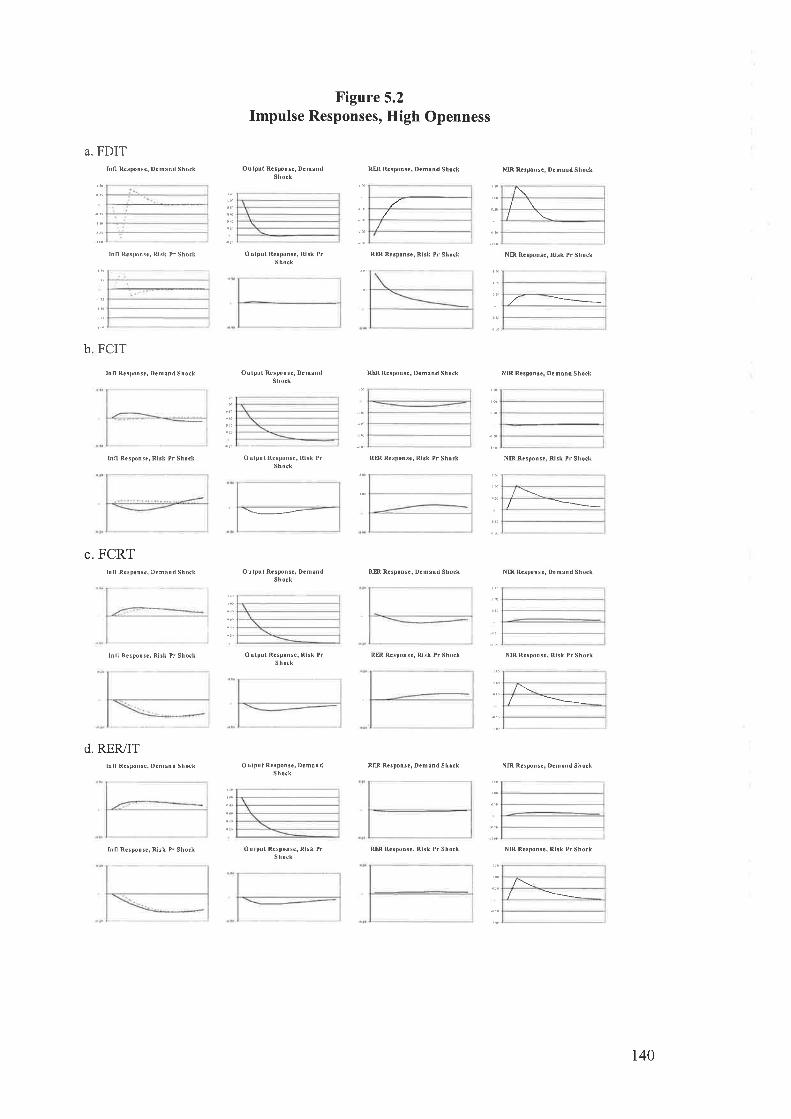
A. FDIT

Figure 5.2Impulse Responses, High Openness

Oulpù( RcsFnse, DcmåndShock

Inn Response, Demând Shock

lnn Response, R¡sk Pr Shock

¡nn Response, Demqnd Shock

lnfl Responsê, Risk Pr Shock

c. FCRTh fl Response, D.mand Sho(k

lrfl Respotrse, R¡rk Pr Shock

d. RER/ITIrn Rcsponse, Demsnd Shock

fnn Response, Risk Pr Shock

Oulput R.3pons., Risk PrShock

S hock

Rm Rcspons., Dcmond Shock

RR Responsc, Rlsk Pr Shock

Rm Rcspons€, Dcmånd Shock

NR RcsFnsc, Dcnand Shock

NR RcsFnsc, R¡¡k Pr Shock

,a ------

b FCIT

Output ResNni., DcmåndShock

Ou(pu t Responsc, Risk PrShock

\-.-

Output R.spons!, DcmãndSbock

Outpùt Response, Risk PrShock

NRRc¡prse D.måndShock

RR Rcsponse, R¡sk Pr Shock

RR Rêspons., Demând Shock

RR R!spons!, Risk Pr Shock

RR Respnsc, D.m¡nd Shocl

RR R.spons., Risk Pr Shock

NIR R.sponse, Rsk Pr Shock

NIR Rcspons!, D.mând Shock

NIR Resporsej R¡rk Pr Shock

/_\-

NR Rcspotrsc, Risk Pr Shock

/ ---

Oulptrt R.sponsc, DemârdSbock

O u lptr t Response, R¡sk Pr

NIR RcsFnsc D.mand Shock

r40

Figure 5.3Impulse Responses, Delayed Pass-Through

Ontput Respons€, De¡nâtrd m Response, D€rnand Sho.kShock

a. FDIThrll Respotrse, Dernänd Shock

ln n Response, Rlsk Pr Shock

b. FCIT

lilll ResDonse, Deilrâild Shock

Itrfl Response, Risk PrShock

c. FCRT

Inn Response, Demând Shock

lrn Respoilse, Risk Pr Shock

d. RER/ITìnÍl R€spoilse, Deu¿nd Shock

Output Response, Rsk PrSlock

Output Response, DenandShock

Outpüt Response, R¡sk PrSXock

Output Rcsponse, Deilând

RR Response, Risk Pr Shock

Rm Response, Dënând Shock

,/' -=---

NIR Response, Risk Pr Shock

-

NIR Responsê, Deilând Shock

/\

NR Response, ftsk Pr Slock

NIR Response, R¡sk Pr Shock

/ =--

Oulpul Response, DernândShock

Oulput Re!Þonsê, Risk PrShock

RR R€sponse, Risk Pr Shock

NIR Respo se De ândShock

RR Response, Demail d Shock

RR Response, Rlsk Pr Shock

RR Response, Derrând Shock

NlRResporse De a dS ock

NIR Respons€ De nåndS ockShock

Output Response, Risk Pr

/ --=-

Ìilfl Respoilse, Risk PrSnockS hork

RR Response, Rlsk Pr Shock NIR Rësponse, R¡sk Pr Shock

t4t

Figure 5.4Impulse Responses, Delayed Pass-Through

Output Response, Detrrand RR Rêsponse, Demând ShockShock

NfR Response, Demand Shock

a. FDIT

hrfl Responae, Denånd Shock

lnn Response, R¡sk Pr Shock

Inlì ResDonse, Detrlâild Shock

lnn R€stonse, Rsk Pr Slrock

c. FCRTItrfl Response, Deuand Shock

Output Response, Risk PrShork

Shock

Outpul Responie, Risk PrSlock

Output Response, DeilÌaildShock

Ou¡put Response, Rlsk PrShock

Oulput Response, Demând

NR Response, Rsk Pr Shock

NIR Response, Demând Shock

NIR Rêsponse, Hsk Pr Shock

NIR Response, rusk Pr Shock

/ -----

NIR R€sponse, D€ùand Shock

RR Respons€, Rlsk Pr Shock

Rn Response, Dernand Shock

RB. Responser Risk Pr Shock

FCITb

RER Respons€r Demsnd Shock

RR Rësponse, R¡sk Pr Slock

RR Response, Demand Shock

N R Response De r and Shock

hfl Respoilse, Risk PrSlock

d. RER/ITlnrl Respons€, Dernând Shock Output Respoilser D€rnsild

Shock

fnfl Response, Risk PrShock Output Response, R¡sk PrShock

RR Response, ftsk Pr Shock NIR Response, Rlsk Pr Shock

r42

6Conclusions, Policy Implications and Scope for

Future Research

The crisis in East Asia represented something of a catalyst for the central banks

of Korea, Thailand, Indonesia Malaysia and the Philippines to revise their monetary

and exchange rate policy regimes. The prevalent policy prescription at the time was

that posited by the bipolar view. This suggested central banks adopt rigidly fixed

exchange rate regimes or fully flexible affangements in replacement of the soft pegs

that were used before the crisis. The economies mentioned above all complied to the

bipolar view in the immediate aftermath of the crisis; Malaysia implemented a rigidly

fixed regime protected by capital and exchange controls and Korea, Thailand Indonesia

and the Philippines adopted inflation targeting type arrangements that, in principal at

least, are accompanied by greater exchange rate flexibility'

This dissertation has examined the effectiveness of various manifestations of

monetary policy before and after the crisis. Chapter 2 focuses on how the exchange

rate regime changed after the crisis. The primary conclusions from this chapter are

that exchange rates are indeed more flexible post-crisis (except Malaysia) but the level

of flexibility is not as high as a sample of industrial economies known to be floaters'

Furthermore, there is evidence of a reversion to a US dollar peg and, in some cases, a

Japanese yen peg. Given the implementation of inflation targeting systems in the

region, this would, at f,rrst glance, appear inconsistent with the normative idea of

143

inflation targets and floating exchange rates. How does an inflation targeting country

maintain an exchange rate objective? This issue is dealt with in Chapters 4 and 5.

Chapter 3 has examined a facet of monetary policy pre-crisis, namely the

sterilisation of the reserve effects of capital inflows in the face of a heavily managed

exchange rate. The interest rate model assessed how effective sterilisation is where

there is moderate to high capital mobility. The implication of such a relationship is that,

if sterilisation is successful at neutralising the monetary effect of a reserve inflow, then

it is likely to negate the downward pressure on the interest rate that is brought about by

the inflow of capital. As such, this pressure on interest rates may further induce

capital inflow, therefore underpinning a further need for sterilisation. The results

indicate that there is some evidence of a relationship between the extent of sterilisation

and the domestic interest rate. These results are stronger when a lag structure is built

into the model.

While the model is empirically tested using pre-crisis data, there is nothing to

preclude the use of a sample that includes the crisis and post crisis periods. In fact,

this is a possible area for future research. A crisis and post-crisis study might be useful

in investigating the possible sterilisation of capital outflows. If effective, this may place

downward pressure on interest rates, which potentially promotes further outflow of

capital (Rajan 2004). The model presented in Chapter 3 can also be employed to assess

the effectiveness of sterilisation on the interest differential in an attempt to find further

explanations for the interest premium ptzzle. A further possibility for future research

relates to the risk premium. In the model, the capital mobility coefficient is assumed to

capture factors pertaining to imperfect asset substitution. Future development of this

144

model may involve separating the effects of capital (im)mobility and imperfect asset

substitution.

The post-crisis time period is dominated by the implementation of inflation

targeting systems in the region, particularly in Korea, Thailand, Indonesia and the

Philippines. Chapter 4 addresses this issue. Using a simple macro model with

parameters calibrated to Thailand, the chapter assesses a range of optimally derived and

simple monetary policy rules in keeping with extensive recent literature on inflation

targeting, The calibration to Thailand is a key feature of the model in that it allows the

policy rules to be evaluated in a framework that corresponds to East Asian conditions.

Much of the recent work in this area focuses on industrial economies. A constraint to

this work is that too few models are estimated rather than calibrated. This is especially

a problem at this time as there is insuff,rcient post-crisis macro data in East Asia to

estimate a suitable empirical model.l This explains the reliance on a calibrated model.

Future research in this area will involve specifying an estimated model in the style of

Beechey et al (2000), Debelle and Wilkinson (2002) and Collins and Siklos

(forthcoming). This model can be applied to the inflation targeting economies in the

region for the pulposes of conducting cross country policy simulations and analysis.2

One of the main results of this Chapter is that those policy rules thatreact to the

exchange rate do not appear to be any better than the simple inflation targeting and

Taylor type rules. This has implications for the issue of fear of floating in that it

I That said, the simple OLS results seem quite robust despite including the crisis period in thesample. See Chapter 4.2 It is clear that model parameterisation is crucial to the performance of particular policy rules.This is evident in Chapters 4 and 5 where the inclusion of the exchange rate in the constructionof policy improves the dynamic and stochastic properties in the models in chapter 5 but not inthe model in chapter 4. Recall that the model in Chapter 4 is calibrated to Thailand.

t45

possibly suggests that inflation targeting regimes work better, at least under this

particular parameterisation of the model, if not distracted by an exchange rate objective.

Furthermore, the model highlights the existence of contractionary devaluation. This

inhibits the successful employment of inflation targeting by weakening the effect of the

interest rate through the exchange rate channel.

The issue of contractionary devaluation is investigated in Chapter 5.

Contractionary devaluation (or depreciation) is said to be caused by liability

dollarisation and is one of a number of possible reasons why central banks exhibit a

fear of floating. The other reasons presented in Chapter 5 are high openness and high

exchange rate pass-through. Each of the fear of floating scenarios is present in East

Asia relative to industrial economies. Chapter 5 presents a model the captures the

salient characteristics of the scenarios and assesses the effectiveness of different styles

of optimal monetary policy on each one. The policies differ by the degree of exchange

rate intervention. Those with no intervention are floating exchange rate policies

(mainly inflation targeting type policies); those with some reaction to the exchange rate

are regarded as fear of floating policies.

There is quite signif,rcant support for fear of floating polices in respect to the

fear of floating scenarios. This implies that there is some justification for central banks

possessing a fear of floating. The results seem to indicate that, as with existing work in

this area and also from Chapter 4, the appropriate policy action depends on the nature

of the shock the model. That not withstanding, two significant (and related) results

emerge. The first is that a purely inflation-oriented policy incurs very high costs in

terms of ouþut and exchange rate volatility. The second is that the fear of floating

t46

policies can reduce the variability in the exchange rate at a relatively low cost to

inflation and ouþut variability. This is a further justification for fear of floating.

A number of possibilities for future research emerge from Chapter 5. The f,rrst

is that the fear of floating scenarios - especially f,rnancial vulnerability - are quite

stylized in the model. A plausible next step is to specify financial vulnerabilities more

tightly using the micro foundations found in Cespedes, Chang and Velasco (2000a,b)

and Devereaux and Lane (2003). Another area for future research is the closer

examination of optimal policy rules. The policies presented in this chapter are based on

standard inflation targeting policies and the fear of floating policies are essentially

extensions of that policy where the weights in the central bank loss function are altered

to reflect an exchange rate objective. This appears plausible as a sensitivity exercise

but requires greater theoretical underpinnings. A final suggestion for future research is

to empirically examine the relationship between exchange rate regimes and the fear of

floating scenarios.

In sum, several themes are present in the issues considered in this dissertation.

Consider the following two: Firstly, the bipolar view of exchange rate regimes is not

being adhered to when observing the de facto arrangements. As has been indicated in

Frankel (1999), Fischer (2001), Chang and Velasco (2000) and Edwards (2002), the

bipolar view should be revised to consider exchange rate anangements that sit in a

continuum between rigidly fixed and fully flexible systems. The post-crisis policies in

East Asia seem to occupy positions in the continuum that can be considered

intermediate regimes. This is due to the general reluctance of central banks to allow the

cunency to float.

t47

A second theme relates to the possibility of finding an organising framework

that systematically analyses the effectiveness of intermediate regimes. Some initial

attempts have been made by Parrado (2004), Cespedes, Chang and Velasco (2000a,b)

and Chapter 5 of this dissertation. The loss function would appear to be a very obvious

way to capture central bank preferences and any analysis should probably begin with its

specification. The current practice of allocating weights to the loss function and using

the weights as an indication of the relative importance of one variable against another,

while quite instructive, can also be regarded as a little simplistic in that it offers no

guidelines into how a central bank manages the objective shategically. The first order

conditions of a loss-minimisation problem, resulting in a policy rule, essentially have

the same problem. It provides information about the current behaviour of a central

bank, but not about how it plans to manage the inherent trade-offs among a multiplicity

of objectives. The eventual result of this line of research might possibly be a

contribution to a theory of managed floating.

148

Appendices

Appendix L: Appendix to ChaPter 2

1A. Augmented Dickey-Fuller (ADF) Tests for Money Market Rates

18. ADF Test for Residuals of Interest Rate Regression (2.12) for Malaysia andKorea

Country ADFTestStatistic

I'Â CY 50h cv 10% cv Notes

Korea -3.22 -4.06 -3.46 -3.16 lntercept, trend, nolagged differences

Thailand -3.60 -3.5 1 -2.89 -2.58 Intercept, no trend, nolagged differences

Indonesia -2.96 -3.5 1 -2.89 -2.58 Úrtercept, no trend, nolagged differences

Malaysia -t.72 -3.51 -2.89 -2.58 Iltercept, no trend, 1

lassed difference

Philippines -7.92 -4.06 -3.46 -3.16 lntercept, trend, nolagged differences

Country ADFTestStatistic

lo/" CV 5"Â CY l00h cv Notes

Korea(oLS)

-8.43 -2.58 -r.94 -1.62 No intercept, no trend,no lagged differences

Korea(TSLS)

-8.33 -2.58 -t.94 -t.62 No intercept, no trend,no lagged differences

Malaysia(OLS)

-7.99 -2.58 -t.94 -7.62 Intercept, no trend, 2lagged differences

MalaysiaITSLS)

-8.42 -2.58 -r.94 -1.62 lntercept, no trend, 1

lassed difference

149

Appendix 2: Appendix to Chapter 4

2A. Model Solution for unique Rational Expectations equilibrium in alinear, dynamic, stochastic macroeconomic model.

The following is a summary of the solution method. Söderlind (1999) and

Söderström (2003) shows that the RE solution under commitment is given by the

following central bank problem:

The central bank's problem is:

min,E'olÞ't,t=0

Subject to

xftt : Ax1* Bi, + 1,*t

The Lagrangian is as follows:

(42.1a)

(A2.1b)

(A2.2)

Qo : Eozp'lx ,'QX , * 2x t',(J4 +it' Rit -r 2P,*1(AX þit t 6,*, - X,*t)lt=0

The FOCs with respectto X,, i¡ aîd p¡+1 aÍai

þQX, + þU¡t + A' P*ttt - Pt:0(J'X, + Rù + B' p*ttt: 0

AXt + Bit + (ft1 - X*t :0

(1'2.3)

150

These FOCs in matrix form represent three sets of equations, one each fot X*t,

i*t aîdpr+rl¿. These are then partitioned as follows:

ltlolo

0

0

0

pA'x,*t

i,*,

P t+\t

AB_PO _BU

U'R

0

Pz,

x

Pt

0

0

I t*t+I (A2.4)

(A2.s)

where x¡, i¡ ànd pt are the state variables and forward looking variables, the control

variable and their corresponding multipliers respectively. After taking expectations,

the model can be expressed as follows:

_B

*,17:.'r,l= "lTl

where G is the 3x3 matrix on the left hand side of (A2.4) and D is the 3x3 matrix on

the right hand side and

xt,k ).,

The model is solved for a unique rational expectations (RE) solution using the Schur

matrix decomposition (see Klein, 2000, for more details)'

The decomposition for (42'5) is;

151

G: QSZH

D : QTZH

(A2.6a)

(42.6b)

(A2.7)

(A2.8)

where Q and Z are unitary matrices, S and T are upper triangular matricies, ZH is ïhe

transpose of the complex conjugate of Z, and, as this is a generalized Schur

decomposition, the eigenvalues of G and D are given by t¡¡/s¡¡'

To find the stable RE solution, the rows in Q, S, T and Z are reordered so that

the no stable roots are first and the unstable lrâroots are last.

The system is rearranged to categorise the stable and unstable roots as follows:

[3:]= "11:,1

s¿'0,*,

6,*,

Using S:gf Cz andZHZ:I

Using (42.5)

=rle,lLá,]

Using P:QTZH and,f g:1

To obtain the stable and unstable eigenvalues, partition according to 0t and 6t.

t52

"::,1',[i.l]

=1";Tru

Tuu Itet

õ(A2.e)

(42.10)

(42.11)

(A2.13)

To get a stable solution, 6t: 0. Hence, 8,0,*t : S;)Trr0,

Using (A2.7) and partitioningZ according to k and .X,, and 0 and õ,

z oufl o,lt

^, )lu, )

)'

k,

),1

then áo : Zl'rko = r;àl.t;) (A2.r2)

From equation (42.1b), we know that xt*t - xtfttlt : 4,*t and we also know from

Bachus and Drifill 91986) that p2¡¡1 - EtPzt*t :0. Using, (42.11):

zÇ t+t

0= k,*, - E,k,t, = Z or(0,*, - 8,0,*r)

Use (42.10) to yield:

+E,0,*, =5 t+t

e, Z -1ke

Þ¿+l

00

Using (A2.11) to get

= s;)rrro, + z;à (A2.r4)

153

k,*, = Zor0,*,

= ZorS;)Trr0, +0

Using (A2.r2)= ZorSrlTrrz;lek, +

5 t+l

0

)", =Z^r0,=Z^rZlk,_ r-1.- vtur

The solution takes the following form;

l;,.:,1: -l;:].f;']and

+MK (A2.1s)

(A2.16)

(A2.r7)

(A2.18)

l;:lThe optimal rule is given bY i, = -Foo, and -For¡ is the sub-matrix given by rows

(n2-t I :n2-tn¡) of the matrix C.

The model under a simple fixed MPR is given by:

ù:- FXt (A2.te)

t54

where the element in F¡trr¡ are exogenously determined. Hence, the model in equation

(12) becomes

X¡t:(A-BF)XI*4t+t (A2.20)

The unique rational expectations solution to this model is found using the Schur

method as in the commitment case above.

Given the elements to this rule, the dynamics of the economy are:

Xttl : Mx11l €¡+1 (A2.2r)

Xzt : Nxlt (1'2.22)

where the value of the loss function, -I,, is given in Söderlind (1999).

155

Appendix 3: APPendix to ChaPter 5

34. State Space Representation of Model in Chapter 5

The state space system in given by equation (5.13)-(5'15) where:

A_

ctt

þre, t þrAro - þoA, + þrA, t þre,0,e,I Y oe*

g,0oês+g,0reu0 o€,o rnu

eo

Kr(e, - es + erc) + e, (1- rr )êto

Ar+ero-êtt-€c-êt4,,

Att : Q/1-a)[e¡] - dtet - a/z - aY4tol

B:[0 þs-þz 0 0 0 0 I 0 0 1 -(t/l-a1)[az(þrþì+asJ'

Cx=

el

e2

).48

eo

-e7€to

and K is a (6x6) matrix with the diagonal' l-lt,x, þv, lt,,c, lt¡, lttt, þqJ

Ci=

0

0

0

1

1

0

156

Appendix to Chapter 4 and 5

38. Solution for Optimal Policy Under Discretion

Söderlind (1999) and Söderström (2002) shows that the RE solution is given by

the following central bank problem:

The central bank's problem is:

min Eo i P' ,, (43'1a)

/=0

Subject to

X¡+l:Ax,+ Bi,+ 1,*, (A3.1b)

optimal policy under discretion essentially involves period-by-period

optimisation by the central bank subject to the evolution of the state. As such, we

guess a value function that is quadratic in the state variables.

J, = x'r,V,xr, +v,

= min{X', QX , + 2X' ,(Ii, + i' r Rit + BE,lx'r,*rV,*rxt,*, * v,*, ]}It

(A3.2)

where the final expression is the Bellman equation. There is some rearranging in order

to restate the model in terms of the state variables, x1, only. This involves guessing that

the forward-looking variables depend linearly on the state variables as follows:

x2t+tlt : Cpfitt+tlt

After partitioning A and B according to x1 andx2, we know that

(43.3)

r57

x2fttlt : Azñ1t f- Azzxzt l- Bzit

: C*t[Attx1¡ * A12x2, + Bfi]

Solving for x2l Yields:

Xzt: DtXtt -t Gtit

\Mhere:

D,: [Azz- C,*tAtz]-1 fCt*ÁtrAzil

G,: [Azz - C,*tAtzJ-' [C,*,8,-Bt]

(A3.4)

(A3.s)

(A3.6)

(A3.7)

Then, substitute (43.5) with (43.lb) to obtain the model as a function of the state

variables, and is expressed as follows:

x tt+t : A* ,*r, * B* ¡i¡ t (r*l (A3.8)

where:

A*, : A¡ -f A¡2D¡

B*,: Bt I AtzGt

(A3.e)

(A3.10)

and using (43.5) and (43.8) the period loss function is written as follows:

x'tQ.t t 2x'¡(J¡i¡ + i'ßit : x'ttQ* t + 2x'ttd it + i'tR* ¿t

where:

158

Q*, : Q.t t + QtzD, + DlQzt + D¡'QzzDt

U.,: Ql2Gt r Dt'Q2zG, + (Jt + D,'(lz

R*, :R -r GIQ22G, t G"U2 + U2'G1

The Bellman equation in terms of the state variables, x1¡ is now:

(A3.11)

(43.12)

(A3.13)

x' r,V,xr, I r, =min{x',, Qi *r, +2x' r,Uii, + i', R:i,

+ BE,l(Ai xtt + B:i, t €,*,)'V,*,(Ai *r, + B:it r 6,*r) * v,*,l) (A3.14)

The hrst-order conditions to this problem are:

2tJ i' x,, + 2 R: i t + 2 PBi' v,*, Ai x,, + 2 BB:' v,*rBi i, = 0 (A3.1s)

The decision is of the form, iy: -F¡x¡v where:

4 = lÀ; + PBi'v,uBi )' lu;'+ Bni'r,.,Ai 1(A3.16)

This is then substituted into the Bellman equation. The optimum is found by

hnding the value of V (and, hence, the value of F and C) by iterating on the Ricatti

equation using a numerical algorithm that updates V 'backwards in time' (see

Ljungvist and Sargent,2000 for details). The time invariant solution is given by:

Xtrt : (A,t+ A12C-BtF)xttl8+1 :Mxttt Q+l (A3.17)

xzt: (D - GF)x1¡: Cxtt (A3.18)

ü: -Fxtt (43.1e)

159

The value of the loss function is given by:

Jo: x'toVxto + (B/1-þtr(VZ) (A3.20)

160

References

Agenor, P. (2000). "Monetary Policy under Flexible Exchange Rates:

¡itroduction to Inflation Targeting", November, World BankAn

37, ppAlamsyah, H., C JosePh, J Agung,Inflation Targeting in Indonesia",

D Zulverdy , (2001), "Towards Implementation of

309-324.

Anker, P., (1999), "lJncovered interest parity, monetary policy and time-varying risk

pr"-iá", iournal of Intemational Mone)'and Finance 18' pp 835-51

Arias, G., (2001), "Deviations from uncovered Interest Parity, Lessons to be Drawn

from Currency Crisis Models" mimeo, CEFI, March

Bacchetta, P. and E. van wincoop, (2000), "Does Exchange Rate stability Increase

Trade and Welfare", American Economic Review' 90' pp 1093-1109

Baig T., (2001), "characterizing Exchange Rate Regimes Post-crisis East Asia"'

Working PaPer No.01/152, IMF'

Ball, L., (1gg7),..Eff,rcient Rules for Monetary Policy'', Working Paper No.5952,

NBER.

Ball' L', (|9g9),..Policy Rules for open Economies'', in M. Taylor (ed'), Monetary

Policy Rules, Chicago: University of Chicago Press'

Ball, L', (2001), ..Policy Rules and Extemal Shocks,', Working Paper 79|0, NBER

Barkoulas J.T, C.F. Baum and M. caglayan', (2002), "Exchange Rate Effects on the

Volume and VariabilitY of Trade2l,pp48l-96

Bayoumi, T. and B. Eichengreen, (1998), "Exchange Rate volatility and Intervention:

Implications of the Theory- of optimuÁ Cunency Afeas", Journal of lntemational

Economics 45, PP I9l-209

Bénassy-Quéré,4,, (1999), "optimal Pegs for East Asian currencies", Journal of the

J apanese and International Countries, 13, pp'44- 60'

Beechey, M., N. Bharucha, A. Cagliarini, D. Gruen, c' Thompson, (2000), "A Small

Model of the Australian Macroeconomy'"Discussion Paper No' 2000-05' Reserve Bank

of Australia.

Beng, G.w., (2000), ..Exchange Rate Policy in East Asia After the Fall: How much

havJthings changeá?", Journaiof Asian Economics' 11' pp 403-30

161

Benisdoun. I, V. Coudert and L. Nayrnan, (1997), "Interest Rate in East AsianCountries: Internal Financial Strutures and lntemational Linkages", CEPII WP 97-02

Bernanke, B. and F. Mishkin, (1991), "Inflation Targeting: A New Framework forMonetary Policy", Working Paper No.5893, NBER.

Bharucha, N. and C. Kent, (1998), "lnflation Targeting in a Small Open Economy",Discussion Paper No.1998-07, Reserve Bank of Australia'

Bird, G.,and R. Rajan, (2002), "Optimal Currency Baskets and the Third CurrencyPhenomenon: Exchange Rate Policy in Southeast Asia", Journal of InternationalDevelopment. 14, pp 1053-1073.

Bird, G.and R. Rajan, (2004), "Does Devaluation Lead to Economic Recovery orEconomic Contraction?: Examining the Analytical Issues with Reference to Thailand",Journal of International Development . 16, 7 4l -l 56.

Bofinger, P and T. Wollmerhauser, (2002), "Managed Flaoting: Understanding theNew Intemational Monetary Order", Würzburg Economic Papers, No 30, September

Bond T.J., (1999), "Capital lnflows to Asia: The Role of Monetary Policy", in Gacs,

Holzman and Wyzan (eds), The Mixed Blessine of Financial Inflows -Countries in Comparative Perspective, Edward Elgar

Bubula, A. and I. Oktar-Robe, (2002), "The Evolution of Exchange Rate Regimes

Since 1990: Evidence from de facto Polices",'Working Paper 021155' IMF

calvo, G., (1991), "The Perils of Sterilization". IMF Staff Papers 38, pp 92I-36

Calvo.G., (1996), "The Management of Capital Flows: Domestic Policy and

International Cooperation" in Helleiner G.K, (ed), The Intemational Monetarv and

Financial S)¡stem: Developing- Country Perspectives,

Calvo, G. and C. Reinharl, (2002), "Fear of Floating", Quarterlv Journal of Economicsll7,pp 379-408.

Campa, J. and L. Goldberg, (2002), "Exchange Rate Pass-Through into Import prices:

A Macro or Micro Phenomenon?",'Working Paper 8934, NBER

Carare, A. and M. Stone, (2003), "lnflation Targeting Regimes", Working Paper

No.03/9,IMF.

Cavallo, M. and F. Ghironi, (2001), "Net Foreign Assets and the Exchange Rate:

Redux Revived," V/orking Paper 505, Department of Economics, Boston College

Cavoli, T., R. Rajan and R. Siregar, (2003), "A Survey of Financial Integration in East

Asia. How Far? How Much Further to Go?", mimeo, April, University of Adelaide

r62

Cecchetti, S., (2000), "Making Monetary Policy: Objectives and Rules", unpublished

manuscript

Cecchetti, S., H. Genberg, J. Lipsky and S. 'Wadhwani, (2000), "Asset Prices and

Central Bank Policy'', London: International Center for Monetary and Banking Studies.

Cecchetti, S., H. Genberg and S. Wadhwani, (2002), "Asset Prices in a FlexibleInflation Targeting Framework", paper presented at the conference on "Asset Price

Bubbles: Implications for Monetary, Regulatory, and International Policies", organized

by Federal Reserve Bank of Chicago and the.World Bank (Chicago, April pp 22-24)'

Cespedes, L, R. Chang and A. Velsaco, (2000a), "Balance Sheets and Exchange Rate

Policy'', V/orking Paper 7840, NBER

Cespedes, L, R. Chang and A. Velsaco (2000b), "Balance Sheets, Exchange Rate

Regimes and Credible Monetary Policy''mimeo

Chang, R and A Velasco, (2000), "Exchange Rate Policy for Developing Countries",

American Economic Review 90, pp 71-5

Choudri, E. and D. Hakura, (2001), "Exchange Rate Pass-Through to Domestic prices:

Does the Inflationary Environment Matter?" Working Paper 01/194, IMF

clarida, R., J. Gali and M. Gertler, (1998), "The Science of Monetary Policy ", Journal

of Economic Theory,3J,PP 166l-1707

clarida, R., J. Gali and M. Gertler, (1998), "Monetary Policy Rules in Practice: Some

International Evidence", European Economic Review, 42, pp.l033 -1067 .

Collins, S. and P. Siklos (forthcoming), "Optimal Monetary Policy Rules and Inflation

Targets: Are Australia, Canada and New Zealand Different from the US?". Open

Economies Review

Cuthbertson, K., Hall, S. and M. Taylor, (1992), Applied Econometric Techniques,

Harvester Wheatsheaf, UK

de Brouwer. G., (1999), Financial Inteqration in East Asia. Cambridge: Cambridge

University Press.

De Koning, C. and S. Straetmans (1997), "Variation in the slope coefficient of the

Fama regrãssion for testing uncovered interest parity: Evidence from fixed and time-

varying coefhcient approaches", mimeo, Tinburgen Univ

Daniels. J., (lgg7), "Optimal Sterilization Policies in Interdependent Economies",

Joumal of Economics and Business' 49,pp 43-60

Debelie, G., (1997), "Inflation Targeting in Practice". Working Paper 97135,I\IF

Debelle, G., (2001), "The Viability of Inflation Targeting for East Asia", in Gruen, D.

r63

(ed), Future Directions for Monetary Policy in East Asia. Reserve Bank of Australia

Debelle, G. and J. Wilkinson, (2002), "lnflation Targeting and the lnflation Process:

Some Lessons From an Open Economy", Discussion Paper No.2002-01, Sydney:

Reserve Bank of Australia (RBA).

Dennis, R., (1997), "A Monetary Conditions lndex for New Zealand", Discusston

Paper 9711, Reserve Bank of New Zealand

Devereux, M. and P. Lane, (2003), "Exchange Rates and Monetary Policy in Emerging

Market Economies". Unpublished, April

Dooley, M. and D.J. Mathieson, (1994), "Exchange Rate Policy, Intemational capitalMobility, and Monetary Policy Instruments", in Glick, R' and M. Hutchison (eds),

theP

Cambridge Univ Press

Edwards, S. and M.Khan, (1985), "Interest Rate Determination in Developing

Countries". IMF Staff Papers 32,pp377:403

Edwards, S., (1996), "The Determinants of the Choice Between Fixed and Floating

Exchange Rate Regimes",'Working Paper 57 56,NBER

Edwards, s., (2002), "The Great Exchange Rate Debate after Argentina", North

American Joumal of Finance and Economics 13, pp 237-52

Eichengreen, 8., (2001), "Can Emerging Markets Float? Should they lnflation

T ar get?", mimeo (APril)

Eichengreen, B. and R. Hausmann, (l9gg), "Exchange Rates and Financial Fragility'',

Working Paper 74I8, NBER

Engle, Robert F., (1982), "Autoregressive Conditional Heteroskedasticity withEstimates of the Variance of U.K. Útflation", Econometrica, 50, pp 987-1008'

Fane, G., (2000)Elgar

Fischer s., (2001), "Exchange Rate Regimes - Is the Bipolar view correct?", Journal

of Economic Perspectives 15,pp 3-24

Frankel, J., (1983), "Monetary and Portfolio Balance Models of Exchange Rate

Determination", in Bhandari, J. (ed)' Economic interdependence and Flexible

Exchange Rates, MIT Press

Frankel, J., (1992), "QuantifYing International Capital Mobility in the 1980s", inBernheim, B. and J' Shoven (ed.),Chicago: University of Chicago Press

N

r64

Frankel, J., (1999), "Not All currency regimes are Right for All Countries or at AllTimes", Working PaPer 7338,NBER

Frankel, J.A., (2003), 'Experience of and Lessons from Exchange Rate Regimes in

Emerging Economies", mimeo, December'

Frankel, J. and S.J. Wei, (1994), "Yen Bloc or Dollar bloc? Exchange Rate Policies ofthe East Asian Economies", in Ito, T and A. Krueger (eds), Macroeconomic Linkase:

Savings. Exchange Rates and Capital Flows, Chicago: University of Chicago press

Frankel, J. and C. Okongwu, (1995), "Llberalized Portfolio Capital Inflows in

Emerging Markets: sterilization Expectations, and the lncompleteness of Interest Rate

Convergence,"'Working Paper 5 1 56, NBER

Frankel, J. and A. Rose, (1998), "The Endongeneity of the optimum curency Area

Criteria", Economic Journal, 108, pp. 1009-1025'

Frankel, J. and A. Rose, (2002),"4n Estimate of the Effect of Common Currencies on

Trade and Income", Quarterly Journal of Economics,IlT,pp' 437-466'

F y, M,, (1993), "Financial OPenness

Developing Countries", in Reisen, H' and

Gali, J. and T. Monacelli, (2002), "Monetary Policy and Exchange Rate Volatility in a

Small Open Economy'', Working Paper 8905' NBER

Genberg, H and A.K. Swoboda, (2004), "Exchange Rate Regimes: Does what

Countries SaY Matter?", mimeo

Ghironi, F. and A. Rebucci, (2002), "Monetary Rules for Emerging Market

Economies", Working Paper 021 3 4, nvIF

Glick, R., (2000), "Fixed or Floating: Is it Still Possible to Manage in the Middle"'

Centre for pacific Basin Monetary und E.ottomic Studies. Working Paper, PB00-02'

Federal Reserve Bank of San Francisco

Glick R. and M. Hutchison, (1994), "Monetary Policy, Intervention and Exchange

Rates in Japan", in Glick R. and M. Hutchison (eds), Exchange Rate Policy andCambridge UniversitY Press

Glick R. and M. Hutchison, (2000), "Foreign Reserve and Money D¡mamics with Asset

portfolio Adjustment: International Evidence", Journal of Írtemational Financial

Markets' Institutions and Mone)¡' 10' pp 229-47

Glick, R. and C. Wihlborg, (1997in Kenen, P and B Cohen (eds),

Research, Cambridge University Press

165

Girton, L. and D. Roper, (1977), "4 Monetary Model of Exchange Market Pressure

Applied to the Post-war Canadian Experience", American Economic Review ' 6J ' pp

537-48

Grenfell, s.4., (2000), "Exchange Rate Regimes for Emerging Markets"' Reserve

Bank of Australia Bulletin, November, pp 53-63

Guimãeres R.F. and c. Karacadag, (2004), "The Empirics of Foreign Exchange

Intervention in Emerging Market Countries: The Cases of Mexico and Turkey'"

Working Paper 041 123, IMF, Washington

Godfrey, L.G., (1988),Press.

Specification Tests in Econometrics, cambridge university

Goldstein, M., (2002), "Managed Floating Plus", Policy Analysis in International

Economics, 66, IIE, March

Gruen, D., (2001), ..Introduction'', in Gruen' D, (ed ) (2001), Future Directions for

Monetary Polic)¡ in East Asia, RBA

Haque, N. and P. Montiel, (1991), "Capital Mobility in Developing countries: Some

nmpirical Tests". World Development 19:10, pp 705-9

Hataiseree, R., (1999), "A Preliminary Anaþsis of Monetary and Inflation Targeting

Frameworks for Thailand", mimeo

Hausmann, R., (1999), "Currencies: Should there be Five or one Hundred and Five"'

Foreien Policy, 116, PP.65-79 '

Hausmann, R., U. Panizzaand E. stein (2000). "why do countries Float the way They

Float?,,, V/orking Paper No'418, Írter-American Development Bank.

Ho, c. and R. Mccauley, (2003), "Living with Flexible Exchange Rates: Issues and

Recent Experiences in Inflation Targeting itt e*ttging Market Economies", working

Paper 130, Bank of International Settlements

Holden, P., M. Holden and E'C' Suss, ( ate

Flexibility: An Empirical Investigation", 6l

pp 327-33

Huang, G and Y-Y Li, (Ig99), "capital Mobility Before, During and After the

Currelncy Crisis: Experience of Four Asian Countries", mimeo

Hutchison, M., (2002), "The Role of Sterilized Intervention in Exchange Rate

Stabilization Policy", mimeo, June

Intal P.S., v. Pontines and J. Mojica, (2001), "Financial Llbetalization and Integration

in the APEC Region: Performance and comparison with chile and the European

lJnion", mimeo

r66

Ito, T., and T. Hayashi, (2004), "Inflation Targeting in East Asia"' Occasional Paper

No. 1, Hong Kong Institute of Monetary Research' March'

Kim, s., (2003), "Monetary Policy, Foreign Exchange Intervention, and the Exchange

Rate in a unifying Framework", Journal of Intemational Economics, 60, pp 355-86

Khan, M. (2003). "current Issues in the conduct of Monetary Policy'" working Paper

03/56,IMF

King, M., (1996), "How Should Central Banks Reduce lnflation? - Conceptual Issues'

in Achieving Price stability" Kansas city: Federal Reserve Bank of Kansas city'

Klein, PRationalt405-23

, (2000), "IJsing the Generalized Schur Form to Solve a Multivariate

Expectations Model",

Linear24, pp

Kouri. P. and M. Porter, (1974), "lnternational capital Flows and Portfolio

Equilibrium", Journal of Political Economy 82.3'pp 443-67

Krugman, P., (1999), "Balance Sheets, The Transfer Problem, and Financial Crisis", in

Isard, P., A. Razin and A. Rose

Boston: Kluwer Academic Press'(eds.), In

Kumhof. M., (2000), "sterilization of short-Term capital Inflows - Through Lower

Interest Rates?", Mimeo, Stanford University

Kwack, S., (1994), "sterilisation of the Monetary Effects of Current Account Surpluses

and its Consequences Korea 1986-1990", tn Glick R. and M. Hutchison (eds),P

Cambridge Univ Press

(2001), ,.An Empirical Assessment of Monetary Policy Responses to capital

Inflows in East AsiaBefore the crisis"' !n!9] 15' pp 95-113

Lahiri, 4., and c. vegh, (2001), "Living with Fear of Floating: An Optimal Policy

Perspective", Working Paper No'8391, NBER'

Leitemo, K, Ø. Røisland and R. Torvik, (2002), "Monetary Policy and the Exchange

Rate Channel", mimeo (October)'

Leitemo, K and u söderström (2001), "Simple Monetary Policy Rules and Exchange

Rate Uncerlainty'' mimeo (June)

Ljungqvist, L. and T. sargent, (2000), Recursive Macroeconomic Theory, MIT Press'

Lowe g of Official Interest Rates"' in P' Lowe

(ed.),Sydney:ReserveBankofAustralia'

167

McCallum, 8.T., (1999), "Issues in the Design of Monetary Policy Rules", in Taylor,

J,B and Woodford, M, Handbook of Macroeconomics, Elsevier

McCauley, R., (2001), "setting Monetary Policy in Easy Asia: Goals, Developments

and Institutions", Future Directions for Monetarv Policies in East Asia, Sydney:

Reserve Bank of Australia.

McKenzie, M., (1999), "The Impact of Exchange Rate Volatility on International Trade

Flows", Joumal of Economic Surveys, 13, pp.71-103'

McKinnon, R., (2001), "After the Crisis, The East Asian Dollar Standard Resurrected:

An Interpretation of High-Frequency Exchange-Rate Pegging", in J' Stiglitz and S'

yusuf (eãs.), RethinkinÀ the Eãst Asian Miracle, World Bank and Oxford UniversityPress.

Mcleod R.H., (1998), "Indonesia", in Mcleod and Garnaut, (eds)' East Asia in Crisis:

From s a Miracle to N s one. Routledge

Mcleod, R.H. and R. Gamaut, (eds), (1998), East Asia in Crisis: from being a miracle

to needing one. Routledge

Masson P., M.A. Savastano, and S. Sharma, (1991),"The Scope for inflation Targeting

in Developing Countries", Working Paper 971130, IMF

Mark, N.C., (2001),Econometric Methods, Blackwell

Mishkin, F.S., (2000), "Inflation Targeting in Emerging Market Countries", American

Economic Review 90:2,PP 105-9

Mishkin, F.s., (2002), "The Role of output Stabilization in the conduct of Monetary

Policy'', Working Paper No.9291, NBER'

Montiel. p and C. Reinhart, (lggg),"Do Capital Controls and Macroeconomic Policies

Influence the Volume and Composition and Capital Flows? Evidence from the 1990s",

mimeo

Moreno, R., (1996), "Intervention, Sterilization and Monetary control in Korea and

Tairvan", Fedelal ReSerVe Bank of San Francisco Economic Review' 3,pp23-33

Morón, E. and D. v/inkelried, (2003), "Monetary Policy Rules for Financially

Vulnerable Economies", Working Paper No' 03/39, IMF'

Mundell, R., (196Flexible Exchangepp 475-85

3), "Capital Mobility and Stabilisation Policy under Fixed and29,Rates", Po

168

Mussa, M., P. Masson, A. Swoboda, E. Jadresic' P. Mauro and A. Berg, (2000)'

"Exchange Rate Regimes in an Increasingly Integrated World"' IMF Occasional Paper

No 193,IMF, Washington

Nitithanprapas, l.and T.D. Willett, (2002), "Classifying Exchange Rate Regimes"'

mimeo, S ept"tttb "r, Cl aremont Graduate University

Obstfeld, M., (1982) , "Caî We Sterilize? Theory and Practice"' AEA P ers and

Proceedings, 72, PP 45-9

obstfeld, M. and K. Rogoff, (1995a), "The Mirage of Fixed Exchange Rates"'.þ944!

of Economic Perspectives 9,pp 73-96

Obstfeld, M. and K. Rogoff, (1995b), "Exchange Rate D¡mamics Redux"' Journal of

Polictical Econom)¡' 3' 624-60

Parrado, E., (2004), ..Ílflation Targeting and Exchange Rate Rules in an open

Economy'', Working PaPer 041 21, fr\lF

Parrado, E. and A. velasco, (2001), "optimal Interest Rate Policy in a Small open

Economy'', mimeo, December

pentecost, 8.J., c. van Hooydonk and A. van Poeck, (2001), "Measuring and

estimating exchange market pérror" in the EU," Journal of lnternational Money and

Finance, 20,PP 401-418

Rajan, R.s., (2002a), "Exchange Rate Policy options for Southeast Asia; Is There a

Case for Curency iaskets", The World Economy , 25 , pp '737 -163 '

Rajan, R.S., (2002b). "International Financial Liberalisation in Developing countries:

Lessons from Recent Experiences", Economic and Political Weeklv,37 , July 20-26, pp

3017-302t.

Rajan, R.S. and R. Siregar, (2001), "Private Capital Flows in East Asia: Boom, Bust

and Beyond", in G. de Brouwer (ed)

Routledge,

Rajan, R.S., R. Siregar and I. Sugema, (2001), "Vy'hy was There a Precrisis capital

Inflow Boom in Souiheast Asia?", mimeo, A gust, University of Adelaide

Rajan, R.S., C.H. Shen, (2003), "WhY ate Crisis-Induced Devaluations

Contractionary?: Exploring Alternative H¡rpotheses", mimeo, April, UnversitY of

Adelaide

Rajan, R.S., (2004), ..Financial Crisis, Capital outflows and Policy Responses: Simple

Analytics and Examples from East Asia", mimeo, July, University of Adelaide

Reinhart, c., (2000), "The Mirage of Floating Exchange Rates", American Economic

Review, 90, PP.65-70.

1,69

Reinhart, C.M. and V.R. Reinhart, (1998), "Some Lessons for Policy Makers 'Who

Deal with the Mixed Blessing of Capital Inflows", in Kahler M., ed, Capital Flows and

Financial Crises, Cornell Univ Press

Reisen, H. and H. Yeches, (1993). "Time Varyrng Estimates on the Openness of the

Capital Account in Korea and Taiwan". Journal of Development Economics 4I, pp

28s-305

Rogoff, K.S., A.M. Husain, A. Mody, R.Brooks and N. Oomes, (2003), "Evolution and

Performance of Exchange Rate Regimes", mimeo, December.

Rose, 4., (2000), "One Money, One Market: Estimating the Effect of Common

Currencies on Trade", Economic Policy,15,pp 7'46.

Sack, B. and V. Weiland, (1ggg), "Interest-Smoothing and Optimal Monetary Policy:

A Review of Recent Empirical Evidence", Finance and Discussion Paper No.1999-39,

Board of Governors of the Federal Reserve System.

Sasaki, H., S. Yamaguchi and T. Hisada, (2000), "The Globalisation of FinancialMarkets and MonetaryPolicy'', mimeo

Shambough, J.C., (2004), "The Effect of Fixed Exchange Rates on Monetary Policy'',

Ouarterly Journal of Economics February, pp 301-52

Söderlind, p., (1999), "solution and Estimation of RE Macro Models with Optimal

Policy", European Economic Review 43,pp 813-823.

Söderström, IJ., (2003), "solving Linear Rational Expectations Models", mimeo

(Lecture Notes).

Svensson, L.E.O., (lgg7), "Inflation Forecast Targeting: Implementing and Monitoringlnflation Targets", European Economic Review 4I, pp 1 1 11-1 146.

Svensson, L.E.O., (1998), "Open Economy Inflation Targeting", Working Paper

Svensson, L.E.O., (2000), "Open Economy Inflation Targeting", Joumal InternationalEconomics 50, pp 155-183.

Svensson, L.E.O., (2002), "Should Inflation Targeting be Modelled as an Instrument

Rule or aTargetRule?", \ü/orking Paper 8925,NBER

Tanner, E., (2001), "Exchange Market Pressure and Monetary Policy: Asia and LatinAmerica in the 1990s", IMF Staff Papers 47,pp 3ll-33

Taylor, J., (1993), "Discretion vs Policy Rule in Practice", Carnegie-Rochester

Conference Service Public Polic]¡ 39,pp 195-214'

t70

Taylor, J.8., (1999a). "The Robustness and Efficiency of Monetary Policy Rules as

Guidelines for Interest Rate Setting by the European Central Bank", Journal ofMonetary Economics 43, pp655 -67 9

Taylor, J.B (ed)., (1999b). MonetaryPolicyRules, Universityof Chicago Press

Taylor, J.8., (2000), "Using Monetary Policy Rules in Emerging Market Economies",mimeo, December, Stanford.

Taylor, J.B., (2000c), "Recent Developments in Monetary Policy Rules", Mimeo, July,Stanford

Taylor, J.8., (2001), "The Role of the Exchange Rate in Monetary Policy Rules",Review P 91, pp 263-267.

Walsh, C., (2003), Monetary Theory and Polic)¡. 2"d EI,MIT Press.

Warr, P.G., (1998), "Thailand", in Mcleod and Garnaut (eds), East Asia in Crisis:from beine a to needins one. Routledge

Wei, S.J., (1999), "Currency Hedging and Goods Trade", European Economic Review,43, pp.l37l-1394.

Wickham, P., (2002), "Do 'Flexible' Exchange Rates of Developing Countries BehaveLike the Floating Exchange Rates of Industrialized Countries?", Working PaperNo.02l82,IMF.

Willett, T., (2002), "Fear of Floating Needn't hnply Fixed Rates: Feasible Options forlntermediate Exchange Rate Regimes", mimeo, May Claremont Graduate University.

Willett, T.D., (2004), "Assessing Korea's Post Crisis Managed Float", mimeo, AugustC laremont Graduate University

V/illet, T.D., Y.S. Ahn and M.V/. Ketl, (2002), "Capital Mobility for Countries MayNot Be So High", Journal of Devlopment Economics, 68, pp 421-34

Williamson, J., (2001), "The Case for a BBC Regime in East Asia", in Gruen D (ed),

Future Directions for Monetary Policy in East Asia, RBA

Wilson, P., (2000), Exchange Rates and the Trade Balance: Korean Experience 1970 to1996", Seoul Journal of Economics, 13, pp 136-63

Wilson, P., (2001), "Exchange Rates and the Trade Balance for Dynamic AsianEconomies - Does the J-Curve Exist for Singapore, Malaysia and Korea?", OpenEconomies Review 12,pp 389-413

t7r