Embed Size (px)
Citation preview
Monetary and Fiscal Policy Rules in the EMU*
Bas van Aarle1, Harry Garretsen2 and Florence Huart3
Abstract
This paper studies the design and effects of monetary and fiscal policy in the euro-area. To do so, a
stylised two-region model of monetary and fiscal policy rules in the EMU is built. It is analysed how
monetary and fiscal rules affect the adjustment dynamics in the model. Both the effects on the
individual countries and on the EMU aggregate economy are studied. Three aspects play an important
role in the analysis: (i) the consequences of alternative monetary and fiscal policy rules, (ii) the
consequences of asymmetries between EMU countries -asymmetries in macroeconomic shocks and
macroeconomic structures-, (iii) the role of alternative degrees of backward and forward-looking
behaviour in consumer decisions and inflation expectations.
Keywords: EMU, Fiscal Policy, Monetary PolicyJEL Code: F31, F41, G15
March 2003
1 LICOS, University of Leuven, Belgium; University of Nijmegen, Department of Applied Economics,University of Nijmegen, the Netherlands and research affiliate at CESifo, Munich, Germany. (email:[email protected] )
2 Utrecht School of Economics, Utrecht University, The Netherlands; Centre for German Studies(CDS), University of Nijmegen, the Netherlands and research fellow at CESifo, Munich, Germany.(email: [email protected] )
3 MÉDEE, Université des Sciences et Technologies de Lille, France. (email:[email protected])
* We gratefully acknowledge the comments by an anonymous referee. The first author acknowledgesthe financial support from the Fonds voor Wetenschappelijk Onderzoek Vlaanderen (F.W.O.).
1
1. Introduction.
With the introduction of the Economic and Monetary Union (EMU) on January 1, 1999, the research
interest in the design, implementation and transmission of monetary and fiscal policy in a monetary
union has gained momentum. This interest can be explained by the fact that EMU has altered in a
fundamental way monetary and fiscal policy design in the EMU countries. Initially, the literature on
EMU concentrated especially on “optimal currency area” aspects, investigating the costs of giving up
national monetary and exchange rate policies in the presence of asymmetric shocks and asymmetric
business cycles, considering also the role of alternative adjustment mechanisms, in particular fiscal
policy and labour market flexibility. More recent are the interests in the design and effects of monetary
and fiscal policies in a common currency area.1
Most importantly, EMU implied the replacement of national currencies by a common
currency and the replacement of national central banks and national monetary policy by a common
central bank, the European Central Bank (ECB) that manages the common monetary policy. The
mandate and operational framework of the ECB are specified in the Maastricht Treaty. Granted a high
degree of independence, the primary objective of the ECB is price stability in the euro-area. The
second objective is securing economic growth in the euro-zone.
The institutional framework of fiscal policy making has been changed also by the EMU.
While fiscal policy remains delegated to the national level, a set of constraints in the form of the
Stability and Growth Pact (SGP) has been introduced. The SGP was adopted in 1997 (Resolution of
the European Council, Amsterdam, June 1997) in order to strengthen fiscal discipline in EMU.2 EMU
Member States commit to avoid “excessive public deficits” and follow a “medium-term objective of
budgetary positions close to balance or in surplus”. Sanctions would apply (public recommendation,
fees) if public deficits are excessive (above 3% of GDP) except in “exceptional circumstances” (as a
real GDP decline of 2 % on an annual basis).3 The SGP provides budgetary guidelines in the medium
term that complement guidelines at the national level.
The SGP also aims at fostering fiscal policy co-ordination through its “Stability Programs”
and multilateral surveillance procedures. Policy co-ordination in the EMU concerns (i) the co-
ordination of national fiscal policies since countries may adopt inadequate fiscal policies because of
externalities and spillovers between EMU countries, (ii) the co-ordination of monetary and fiscal
policies in the EMU since the monetary and fiscal policy mix may be inadequate from the aggregate
EMU perspective because of spillovers between monetary and fiscal policies.
In official statements, the ECB and European Commission emphasise a rule-based
macroeconomic policy framework as the norm for the EMU. It is assumed that it will also provide a
1 See Buti and Sapir (1998) for a detailed overview on EMU.2 Rationales for the SGP can be found e.g. in Artis and Winkler (1997) and Buti et al. (1997).3 European Commission (2000), (2001), (2002) gives details on the provisions and operating of the SGP.
2
consistent framework for effective macroeconomic policy co-ordination: “In the field of monetary-
fiscal policy co-ordination, the emphasis has shifted away from the joint design of short-term policy
responses to shocks towards the establishment of a non-discretionary, rule-based regime capable of
providing monetary and fiscal policy-makers with a time-consistent guide for action and thus a reliable
anchor for private expectations.” And, “In all fields, the Treaty sets up a clear allocation of policy
responsibilities based on a set of shared objectives and guiding principles for the conduct of policies in
Europe, notably stable prices, sound public finances and sustainable non-inflationary growth (Articles
2 and 4 of the Treaty). Central Bank independence and budgetary rules are therefore mutually
reinforcing elements in this framework with a view to ensuring macroeconomic stability”, European
Central Bank (2003).
This paper analyses the design and effects of monetary and fiscal policy rules in EMU,
applying the insights from the recent literature – surveyed in Section 2 − on monetary and fiscal policy
rules. Macroeconomic policy rules are to be seen as systematic responses by the monetary and fiscal
authorities to macroeconomic conditions, using information in a consistent and predictable way.4
Policy rules foster policy transparency and accountability, thereby reducing uncertainty and
contributing to a stable economic environment. On the other hand, it cannot be excluded that policy
rules in certain conditions curtail flexibility to such an extent that the actual policies are largely
inadequate. A crucial underlying assumption in the recent literature on policy rules is that the private
sector perceives the policy rules as credible and assumes that they are followed consistently. In other
words, it is assumed that dynamic inconsistency problems in policymaking have been solved by
appropriate designs.
A macroeconomic policy regime consists of the monetary and fiscal policy strategies that are
implemented. The monetary and fiscal policy strategies are interacting and their joint implementation
affects macroeconomic adjustments. In this paper, a policy regime is characterised by the shape of the
monetary and fiscal policy rules. Even in our simple framework, there are clear interrelations between
monetary and fiscal policy rules: the design of the monetary rule will affect the macroeconomic
conditions, which on their turn affect the fiscal policy reactions, and vice versa. These interactions
point to the crucial issue of macroeconomic policy co-ordination in the EMU.
Monetary and fiscal policy rules in EMU are studied using a stylised two-region model. This
allows us to distinguish between effects on the EMU aggregate economy and on individual countries.
The model is in the spirit of the recent “New Neo-Classical New Keynesian synthesis”. This approach
builds on Keynesian macroeconomics by including forward-looking expectations and nominal
rigidities. It also strongly emphasises the underlying microeconomic foundations and the design of
macroeconomic policy rules, like the well-known Taylor rule for monetary policy.5 In the spirit of the
4 This systematic part of macroeconomic policies that is based on policy rules is also often referred to as the anticipated partof macroeconomic policies, whereas the discretionary, non-systematic part of macroeconomic policies -the policyinnovations- is assumed to be unanticipated by the public.5 For a detailed overview of this approach see in particular Fuhrer and Moore (1995), Leeper and Zha (2000) and Clarida et
3
literature on policy rules, the ECB is modelled as operating a monetary rule geared at stabilising
inflation and output in the euro-area. Fiscal authorities operate a fiscal rule targeted at stabilising
output in their own country, subject to constraints relating to the SGP. Three aspects especially attract
our interests: (i) the consequences of alternative monetary and fiscal policy rules, (ii) the consequences
of asymmetries between EMU countries -asymmetries in macroeconomic shocks and macroeconomic
structures- (iii) the role of alternative degrees of backward-looking and forward-looking behaviour in
consumer decisions and in inflation expectations.
The paper is structured as follows: Section 2 gives a brief overview of the recent literature on
monetary and fiscal policy rules. Section 3 sets out our two-country EMU model with monetary and
fiscal policy rules. Section 4 discusses the simulation results for various shocks and three alternative
regimes for inflation expectations. In section 5 we deal with the implications of instrument smoothing
in our model. Section 6 deals with the efficiency of policy rules. Section 7 concludes.
2. Monetary and Fiscal Policy Rules: An Overview of The Literature.
In the recent monetary policy literature, monetary rules have received a large deal of attention, in
particular following the work of Taylor (1993), (1999a). Taylor (1993) constructs a simple monetary
policy rule that relates the setting of the short-run interest rate by the monetary authorities to the
output gap and deviations of inflation from an inflation target. Empirical research shows that a Taylor
rule is able to explain rather well the actual interest rate adjustments observed. Research by Rudebusch
and Svensson (1999) suggests moreover, that a Taylor rule may provide in many cases a degree of
macroeconomic stabilisation that approaches the degree provided by the optimal rule. In contrast to
the optimal rule, the benchmark Taylor rule provides the simplicity and transparency emphasised in
the literature on rules vs. discretion. The original Taylor rule has been amended by (i) introducing
forward-looking expectations, (ii) adding an interest rate smoothing objective, (iii) adding a money
growth objective.
There is now a consensus on the functional form of the monetary policy rule. Taylor (1999b)
and Woodford (2001) show that for the rule to be stabilising, the interest rate response coefficient to
deviation of inflation from its target should be greater than one. Moreover, interest-rate smoothing is
destabilising if expectations are not rational (Taylor, 1999b). There are however still disagreements or
uncertainties about the value of the coefficients in the Taylor rule (e.g. that may differ across countries
and over time), and about the most adequate measure of the output gap and the equilibrium real
interest rate. First, to compare with the benchmark rule of Taylor (1993) where the coefficients on
inflation and output are 1.5 and 0.5 respectively, a higher value for the interest rate response to output
al. (1999) for the closed economy case. Clarida et al. (2002) and Gali and Monacelli (2002) extend the analysis to a smallopen economy. Rudebusch (2002) analyses the implications of model and data uncertainty and compares outcomes under aTaylor rule with alternative monetary rules, in particular monetary targeting and nominal income targeting.
4
gap would reduce the size of the fluctuations of real GDP around potential GDP but would increase
the size of fluctuations of the inflation rate around its target. Similarly, a higher value for the interest
rate response to inflation would reduce the variability of inflation but at the expense of a greater
variability of real GDP. Thus, there is an inflation-output variability trade-off in the choice of
coefficients. Second, uncertainty about the correct measure of potential output and the equilibrium
interest rate causes indeterminacy in the long-run inflation rate as shown in Taylor (1999b) and
Woodford (2001). Given the possibility of a mistaken measure of the potential output, McCallum
(2001) concludes that the central bank should not respond strongly to the output gap.
The estimation of a Taylor rule for the EMU area has received a considerable interest in recent
empirical literature on EMU (e.g. Gerlach and Smets (1999), Gerlach and Schnabel (2000), Fase
(2001) and Domenech et al. (2001)). Yet, there is some controversy about the adequateness of Taylor
rules in general -and in the case of the euro-area in particular- and the exact specification that is most
accurate from an empirical/econometric point of view.
That also fiscal policy can be approximated by a policy rule, has received less attention so far.
The issue of policy credibility, aspects of policy discretion vs. rules e.g. have found less interest in the
context of fiscal policy. To implement fiscal rules in practice, policymakers have adopted a broad
range of numerical targets and procedures. These targets and procedures are also often seen as
commitment devices to sustain fiscal discipline. European Commission (2001) provides a detailed
overview on the actual budgeting frameworks and procedures in the EU countries. Most budgetary
rules, objectives and guidelines operate on the expenditure side and provide a multi-annual budgetary
framework.
Taylor (2000) points out that a rule based approach towards fiscal policy may be useful and
delivering new insights. He shows how a simple fiscal rule can be used to explain most fluctuations in
fiscal deficits. Taylor’s starting point is the division of the fiscal deficit into a cyclical component and
a structural component. The first part can be interpreted as the systematic response of fiscal policy to
output fluctuations (the so-called automatic stabilisers), the second part contains structural and
discretionary components of fiscal policy. Taylor estimates this fiscal policy rule in order to evaluate
the respective roles of automatic stabilisers and discretionary fiscal policy in stabilising output
fluctuations in the U.S. economy. Fully comparable results for the EMU are not yet available, but
probably useful as well. The EMU context is especially interesting also because the adjustment phase
to EMU during the period 1990-1998, and the actual operation of the EMU since January 1st 1999,
came with specific fiscal rules, laid down in the Maastricht Treaty and the Stability and Growth Pact.
National budgetary rules and institutions need to be consistent with the principles of fiscal
sustainability of the EU Treaty and the Stability and Growth Pact (SGP).
Some studies such as Leith and Wren-Lewis (2000), Mitchell et al. (2000), Chadha and Nolan
(2002), Ballabriga and Martinez-Mongay (2002) also include a component of government debt
stabilisation into the fiscal rules, to account for the need to secure intertemporal solvency in fiscal
5
policies. While such solvency considerations are certainly interesting and relevant, our approach -
which concentrate on short-run adjustment dynamics and macroeconomic stabilisation- ignores the
long run implications from government debt adjustment.
In the related framework of Leeper (1991), monetary policies that counteract inflation raising
the real interest rate when inflation rises (implying that the coefficient on the inflation gap in the
Taylor rule is larger than one), are referred to as “active”. “Passive” or “Ricardian” fiscal policies are
fiscal policies that secure that the solvency constraint of the government is met at all times, typically
by a fiscal deficit that reacts negatively to the level of debt. A combination of an active monetary
policy and passive fiscal policy produces internally stable adjustment dynamics and a unique steady-
state. This is no longer necessarily the case with passive monetary policy and/or active fiscal policies:
in those cases, situations may arise where e.g. runaway inflation and government debt occurs, or
indeterminacy in nominal and real variables is created or where the economy enters equilibrium cycles
with no well-defined long-run equilibrium (see Benhabib et al. (2001)). While such cases with
complicated adjustment dynamics and non-unique steady-states are interesting in themselves, we will
for simplicity focus in our simulation examples in Sections 4 and 5, on cases that are intrinsically
stable and possess a unique steady-state.
3. A Model of Monetary and Fiscal Policy Rules in the EMU.
The model that underlies our analysis of monetary and fiscal policy rules in the EMU is in the spirit of
the recent New Neo-Classical New Keynesian synthesis. This “new normative macroeconomic
research” uses quantitative dynamic stochastic models combining theoretical insights from the new
classical macroeconomics and the new Keynesian macroeconomics combing rational, forward-looking
behaviour and short-run rigidities.
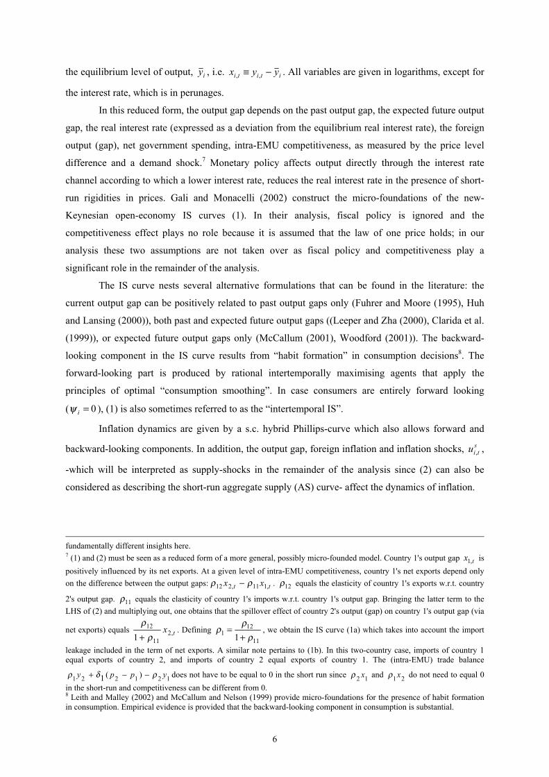
A two-country monetary union is considered. The model consists of a few building blocks: a
goods market equilibrium, inflation dynamics and policy rules. The goods market equilibrium, or IS
curve, of both countries takes the following form:
( ) dttttttttEtttt uppgxrpEixExx ,1,1,21,11,211,1,11,111,11,1 )()1( +−+++−∆−−−+= ++− δηραψψ (1a)
( ) dttttttttEtttt uppgxrpEixExx ,2,1,22,22,121,2,21,221,22,2 )()1( +−−++−∆−−−+= ++− δηραψψ (1b)
in which xi denotes the output gap in country i, i={1,2}6, at time t; iE,t the common nominal interest
rate; pi,t the aggregate price level in country i; gi,t the fiscal balance in country i (a positive value of gi,t
denotes a fiscal deficit); r is the equilibrium real interest rate; dtiu , is an aggregate demand shock
(other than fiscal policy (see (4a,b)). Note that the output gap equals the actual output level, yi,t, minus 6 The two-country monetary union model suffices to analyse the most crucial implications of a monetary union betweencountries. A general n-country framework of a monetary union could have been formulated but would not have delivered
6
the equilibrium level of output, iy , i.e. ititi yyx −≡ ,, . All variables are given in logarithms, except for
the interest rate, which is in perunages.
In this reduced form, the output gap depends on the past output gap, the expected future output
gap, the real interest rate (expressed as a deviation from the equilibrium real interest rate), the foreign
output (gap), net government spending, intra-EMU competitiveness, as measured by the price level
difference and a demand shock.7 Monetary policy affects output directly through the interest rate
channel according to which a lower interest rate, reduces the real interest rate in the presence of short-
run rigidities in prices. Gali and Monacelli (2002) construct the micro-foundations of the new-
Keynesian open-economy IS curves (1). In their analysis, fiscal policy is ignored and the
competitiveness effect plays no role because it is assumed that the law of one price holds; in our
analysis these two assumptions are not taken over as fiscal policy and competitiveness play a
significant role in the remainder of the analysis.
The IS curve nests several alternative formulations that can be found in the literature: the
current output gap can be positively related to past output gaps only (Fuhrer and Moore (1995), Huh
and Lansing (2000)), both past and expected future output gaps ((Leeper and Zha (2000), Clarida et al.
(1999)), or expected future output gaps only (McCallum (2001), Woodford (2001)). The backward-
looking component in the IS curve results from “habit formation” in consumption decisions8. The
forward-looking part is produced by rational intertemporally maximising agents that apply the
principles of optimal “consumption smoothing”. In case consumers are entirely forward looking
( 0=iψ ), (1) is also sometimes referred to as the “intertemporal IS”.
Inflation dynamics are given by a s.c. hybrid Phillips-curve which also allows forward and
backward-looking components. In addition, the output gap, foreign inflation and inflation shocks, stiu , ,
-which will be interpreted as supply-shocks in the remainder of the analysis since (2) can also be
considered as describing the short-run aggregate supply (AS) curve- affect the dynamics of inflation.
fundamentally different insights here.7 (1) and (2) must be seen as a reduced form of a more general, possibly micro-founded model. Country 1's output gap tx ,1 ispositively influenced by its net exports. At a given level of intra-EMU competitiveness, country 1's net exports depend onlyon the difference between the output gaps: tt xx ,111,212 ρρ − . 12ρ equals the elasticity of country 1's exports w.r.t. country
2's output gap. 11ρ equals the elasticity of country 1's imports w.r.t. country 1's output gap. Bringing the latter term to theLHS of (2) and multiplying out, one obtains that the spillover effect of country 2's output (gap) on country 1's output gap (via
net exports) equals tx ,211
12
1 ρρ+
. Defining 11
121 1 ρ
ρρ
+= , we obtain the IS curve (1a) which takes into account the import
leakage included in the term of net exports. A similar note pertains to (1b). In this two-country case, imports of country 1equal exports of country 2, and imports of country 2 equal exports of country 1. The (intra-EMU) trade balance
121221 )(1 yppy ρδρ −−+ does not have to be equal to 0 in the short run since 12 xρ and 21xρ do not need to equal 0in the short-run and competitiveness can be different from 0.8 Leith and Malley (2002) and McCallum and Nelson (1999) provide micro-foundations for the presence of habit formationin consumption. Empirical evidence is provided that the backward-looking component in consumption is substantial.
7
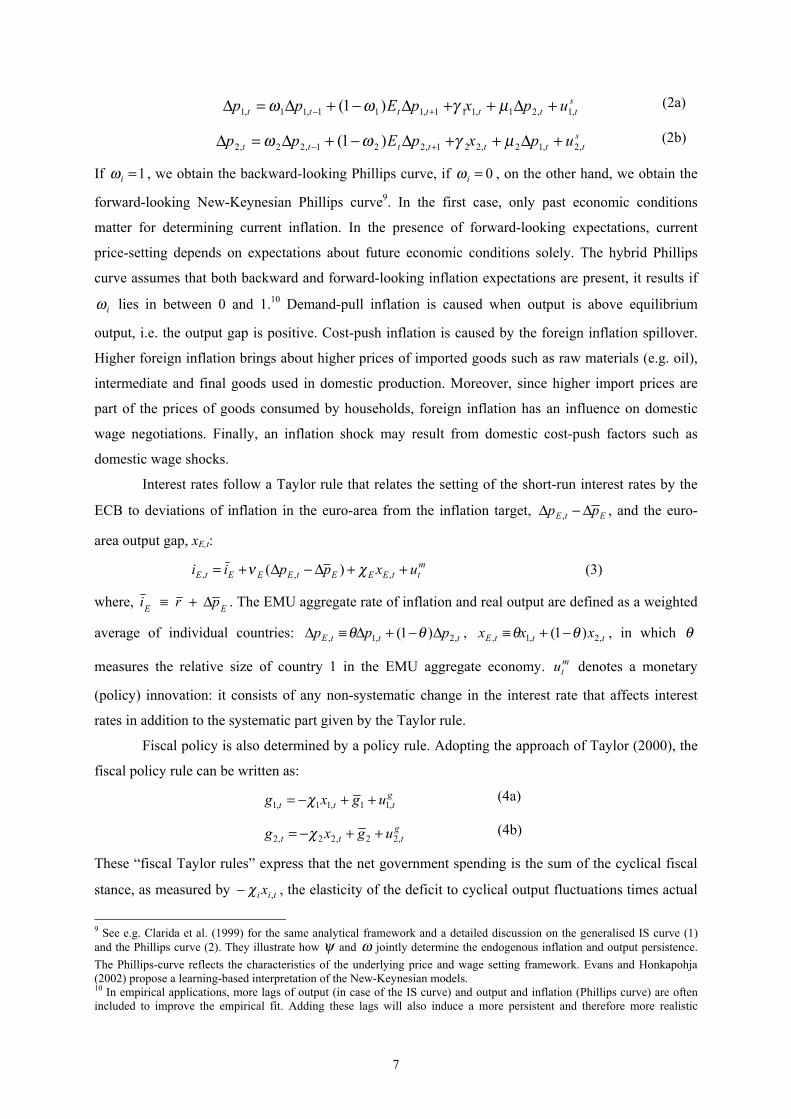
sttttttt upxpEpp ,1,21,111,111,11,1 )1( +∆++∆−+∆=∆ +− µγωω (2a)
sttttttt upxpEpp ,2,12,221,221,22,2 )1( +∆++∆−+∆=∆ +− µγωω (2b)
If 1=iω , we obtain the backward-looking Phillips curve, if 0=iω , on the other hand, we obtain the
forward-looking New-Keynesian Phillips curve9. In the first case, only past economic conditions
matter for determining current inflation. In the presence of forward-looking expectations, current
price-setting depends on expectations about future economic conditions solely. The hybrid Phillips
curve assumes that both backward and forward-looking inflation expectations are present, it results if
iω lies in between 0 and 1.10 Demand-pull inflation is caused when output is above equilibrium
output, i.e. the output gap is positive. Cost-push inflation is caused by the foreign inflation spillover.
Higher foreign inflation brings about higher prices of imported goods such as raw materials (e.g. oil),
intermediate and final goods used in domestic production. Moreover, since higher import prices are
part of the prices of goods consumed by households, foreign inflation has an influence on domestic
wage negotiations. Finally, an inflation shock may result from domestic cost-push factors such as
domestic wage shocks.
Interest rates follow a Taylor rule that relates the setting of the short-run interest rates by the
ECB to deviations of inflation in the euro-area from the inflation target, EtE pp ∆−∆ , , and the euro-
area output gap, xE,t:mttEEEtEEEtE uxppii ++∆−∆+= ,,, )( χν (3)
where, EE pri ∆+≡ . The EMU aggregate rate of inflation and real output are defined as a weighted
average of individual countries: tttE ppp ,2,1, )1( ∆−+∆≡∆ θθ , tttE xxx ,2,1, )1( θθ −+≡ , in which θ
measures the relative size of country 1 in the EMU aggregate economy. mtu denotes a monetary
(policy) innovation: it consists of any non-systematic change in the interest rate that affects interest
rates in addition to the systematic part given by the Taylor rule.
Fiscal policy is also determined by a policy rule. Adopting the approach of Taylor (2000), the
fiscal policy rule can be written as:gttt ugxg ,11,11,1 ++−= χ (4a)
gttt ugxg ,22,22,2 ++−= χ (4b)
These “fiscal Taylor rules” express that the net government spending is the sum of the cyclical fiscal
stance, as measured by tii x ,χ− , the elasticity of the deficit to cyclical output fluctuations times actual
9 See e.g. Clarida et al. (1999) for the same analytical framework and a detailed discussion on the generalised IS curve (1)and the Phillips curve (2). They illustrate how ψ and ω jointly determine the endogenous inflation and output persistence.The Phillips-curve reflects the characteristics of the underlying price and wage setting framework. Evans and Honkapohja(2002) propose a learning-based interpretation of the New-Keynesian models.10 In empirical applications, more lags of output (in case of the IS curve) and output and inflation (Phillips curve) are oftenincluded to improve the empirical fit. Adding these lags will also induce a more persistent and therefore more realistic
8
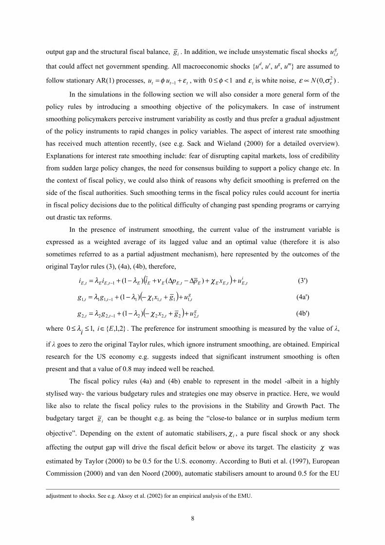
output gap and the structural fiscal balance, ig . In addition, we include unsystematic fiscal shocks gtiu ,
that could affect net government spending. All macroeconomic shocks {ud, us, ug, um} are assumed to
follow stationary AR(1) processes, ttt uu εφ += −1 , with 10 <≤ φ and tε is white noise, ε σε∝ N ( , )0 2 .
In the simulations in the following section we will also consider a more general form of the
policy rules by introducing a smoothing objective of the policymakers. In case of instrument
smoothing policymakers perceive instrument variability as costly and thus prefer a gradual adjustment
of the policy instruments to rapid changes in policy variables. The aspect of interest rate smoothing
has received much attention recently, (see e.g. Sack and Wieland (2000) for a detailed overview).
Explanations for interest rate smoothing include: fear of disrupting capital markets, loss of credibility
from sudden large policy changes, the need for consensus building to support a policy change etc. In
the context of fiscal policy, we could also think of reasons why deficit smoothing is preferred on the
side of the fiscal authorities. Such smoothing terms in the fiscal policy rules could account for inertia
in fiscal policy decisions due to the political difficulty of changing past spending programs or carrying
out drastic tax reforms.
In the presence of instrument smoothing, the current value of the instrument variable is
expressed as a weighted average of its lagged value and an optimal value (therefore it is also
sometimes referred to as a partial adjustment mechanism), here represented by the outcomes of the
original Taylor rules (3), (4a), (4b), therefore,
( ) itEtEEEtEEEEtEEtE uxppiii ,,,1,, )()1( ++∆−∆+−+= − χνλλ (3')
( ) gtttt ugxgg ,11,1111,11,1 )1( ++−−+= − χλλ (4a')
( ) gtttt ugxgg ,22,2221,22,2 )1( ++−−+= − χλλ (4b')
where }2,1,{ ,10 Eii ∈≤≤ λ . The preference for instrument smoothing is measured by the value of λ,
if λ goes to zero the original Taylor rules, which ignore instrument smoothing, are obtained. Empirical
research for the US economy e.g. suggests indeed that significant instrument smoothing is often
present and that a value of 0.8 may indeed well be reached.
The fiscal policy rules (4a) and (4b) enable to represent in the model -albeit in a highly
stylised way- the various budgetary rules and strategies one may observe in practice. Here, we would
like also to relate the fiscal policy rules to the provisions in the Stability and Growth Pact. The
budgetary target ig can be thought e.g. as being the “close-to balance or in surplus medium term
objective”. Depending on the extent of automatic stabilisers, iχ , a pure fiscal shock or any shock
affecting the output gap will drive the fiscal deficit below or above its target. The elasticity χ was
estimated by Taylor (2000) to be 0.5 for the U.S. economy. According to Buti et al. (1997), European
Commission (2000) and van den Noord (2000), automatic stabilisers amount to around 0.5 for the EU
adjustment to shocks. See e.g. Aksoy et al. (2002) for an empirical analysis of the EMU.

9
as a whole. However, they vary between 0.3-0.4 for the Mediterranean countries to 0.8-0.9 for the
Nordic countries. In addition, the degree of fiscal smoothing, iλ , determines the persistence of the
adjustment of the fiscal deficit towards its target. In particular, cases where the fiscal deficit
approaches the ceiling of 3 percent of GDP, fiscal policymakers are likely to become more cautious
and eager to smooth the deficit. Also for other reasons -institutional reasons e.g.- deficit smoothing
may be practised by the fiscal authorities. Ballabriga and Martinez-Mongay (2002) find values for the
fiscal smoothing parameter to range between 0.47 for Belgium and 0.87 for the case of Ireland.
Finally, our specification of the monetary policy rule applies to a closed EMU-wide economy
as opposed to open-economy policy rules that include the exchange rate. Taylor (2001) reviews the
literature on these rules and estimates one for the euro-area. He finds that these rules do not perform
much better than rules without the exchange rate in stabilising inflation and output. The reason is that
closed-economy policy rules already entail the reaction of the interest rate to the exchange rate via an
implicit indirect effect, namely the impact of exchange rate changes on inflation and output.
Moreover, there could be large harmful swings in short-term interest rates if there were a strong direct
reaction of interest rates to temporary fluctuations of the exchange rate.
4. Macroeconomic Adjustment in the EMU: A Simulation Analysis.
This section uses simulations to illustrate the main insights that can be obtained from the model of
Section 3. We simulate the effects of monetary innovations (case (i) and (ii)), supply shocks (case
(iii)), fiscal shocks (case (iv)) and demand shocks (case (v) and (vi)). We consider cases where the
shocks are symmetric (case (i), (ii) and (v)) and asymmetric (case (iii), (iv) and (vi)) and, moreover,
cases where countries are structurally symmetric (case (i), (iv), (vi)) and asymmetric (ii), (iii), (v)).
In these simulations we in particular want to obtain insights into: (i) the consequences of
alternative monetary and fiscal policy rules, (ii) the consequences of asymmetries between EMU
countries -asymmetries in macroeconomic shocks and macroeconomic structures-, (iii) the role of
alternative degrees of backward and forward-looking in consumer decisions and inflation expectations.
To do so, a number of different structural settings and macroeconomic shocks are considered. The
shocks that are analysed are also often considered in macroeconomic simulations with larger scale
macroeconomic models studies (see e.g. Roeger and in 't Veld (2002), Hunt and Laxton (2002),
Dieppe and Henry (2002) for the EMU case) and can be seen as a sort of benchmark to evaluate the
effects of macroeconomic shocks and the resulting adjustment.
All shocks are unanticipated and incur at period 0. Algorithms are readily available to obtain
numerical solutions to our small model, both in case of fully rational expectations and in case of
(partially) backward-looking expectations, see e.g. Fisher (1982) for an extensive methodological
overview. To solve the model, model consistent expectations are imposed in the algorithm that derives
the forward-looking solutions. The Stacked Newton solution method is used, which is known for its
10
fast convergence and robustness in calculating the solutions for smaller scale models with rational
expectations.
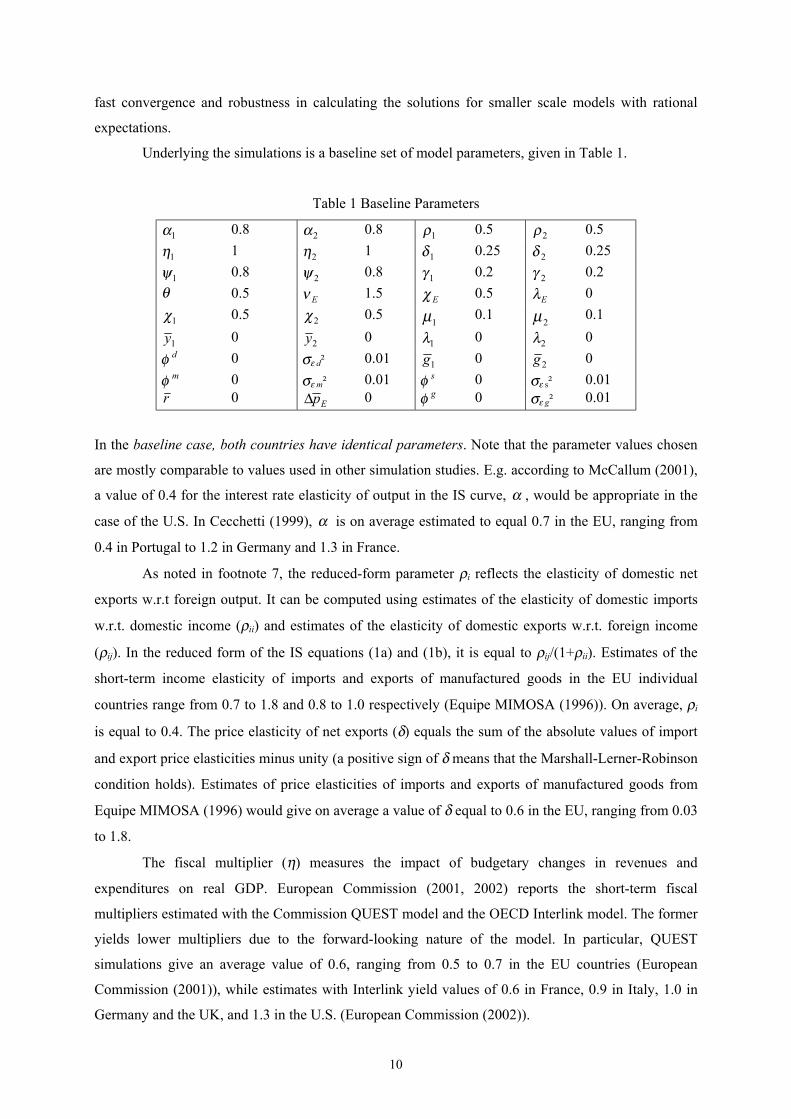
Underlying the simulations is a baseline set of model parameters, given in Table 1.
Table 1 Baseline Parameters
1α 0.8 2α 0.8 1ρ 0.5 2ρ 0.5
1η 1 2η 1 1δ 0.25 2δ 0.25
1ψ 0.8 2ψ 0.8 1γ 0.2 2γ 0.2θ 0.5 Eν 1.5 Eχ 0.5 Eλ 0
1χ 0.5 2χ 0.51µ 0.1
2µ 0.1
1y 0 2y 0 1λ 0 2λ 0φ d 0 σε d² 0.01 1g 0 2g 0φ m 0 σε m² 0.01 φ s 0 σε s² 0.01r 0 Ep∆ 0 φ g 0 σε g² 0.01
In the baseline case, both countries have identical parameters. Note that the parameter values chosen
are mostly comparable to values used in other simulation studies. E.g. according to McCallum (2001),
a value of 0.4 for the interest rate elasticity of output in the IS curve, α , would be appropriate in the
case of the U.S. In Cecchetti (1999), α is on average estimated to equal 0.7 in the EU, ranging from
0.4 in Portugal to 1.2 in Germany and 1.3 in France.
As noted in footnote 7, the reduced-form parameter ρi reflects the elasticity of domestic net
exports w.r.t foreign output. It can be computed using estimates of the elasticity of domestic imports
w.r.t. domestic income (ρii) and estimates of the elasticity of domestic exports w.r.t. foreign income
(ρij). In the reduced form of the IS equations (1a) and (1b), it is equal to ρij/(1+ρii). Estimates of the
short-term income elasticity of imports and exports of manufactured goods in the EU individual
countries range from 0.7 to 1.8 and 0.8 to 1.0 respectively (Equipe MIMOSA (1996)). On average, ρi
is equal to 0.4. The price elasticity of net exports (δ) equals the sum of the absolute values of import
and export price elasticities minus unity (a positive sign of δ means that the Marshall-Lerner-Robinson
condition holds). Estimates of price elasticities of imports and exports of manufactured goods from
Equipe MIMOSA (1996) would give on average a value of δ equal to 0.6 in the EU, ranging from 0.03
to 1.8.
The fiscal multiplier (η) measures the impact of budgetary changes in revenues and
expenditures on real GDP. European Commission (2001, 2002) reports the short-term fiscal
multipliers estimated with the Commission QUEST model and the OECD Interlink model. The former
yields lower multipliers due to the forward-looking nature of the model. In particular, QUEST
simulations give an average value of 0.6, ranging from 0.5 to 0.7 in the EU countries (European
Commission (2001)), while estimates with Interlink yield values of 0.6 in France, 0.9 in Italy, 1.0 in
Germany and the UK, and 1.3 in the U.S. (European Commission (2002)).
11
Our IS curve specification allows for both backward-looking and forward-looking behaviour.
Leith and Wren-Lewis (2001) calibrate a backward-looking IS equation in a small open-economy
macroeconomic model for the UK economy and set ψ equal to 0.9. We follow Batini and Haldane
(1999) who calibrate a small open-economy model for the UK and also specify an IS equation with
both backward and forward-looking behaviour. They note that a value of ψ of 0.8 is empirically
plausible. The parameter γ measures the slope of the Phillips curve and constitutes an important
parameter since it reflects the rigidities in the price adjustment dynamics and thus represents an
important determinant of the short-run adjustment of prices and aggregate supply. This value is also
assumed by Batini and Haldane (1999), and is between other calibrated values of 0.1 (Leith and Wren-
Lewis (2001) for the UK; Rotemberg and Woodford (1999) for the US) and 0.3 (McCallum and
Nelson (1999b) for the US; Gali and Monacelli (2002) for a small-open economy). Gagnon and Ihrig
(2002) estimate the import price pass-through parameter iµ and find it to lie between 0.05 and 0.25 for
most OECD countries. Here we use the value of 0.1 that they also apply in their simulations. Note that
a high value of this inflation spillover can generate instability in the inflation dynamics.
Finally, the values of iχ , which measures the sensitivity of the fiscal deficit to cyclical
variation, are the same as the ones found by the EU Commission (2001) for the euro-area. Setting to
zero the target value for the structural fiscal deficit ig implies an objective of a balanced budget in
accordance to the SGP. The parameters of the Taylor rule are the ones originally proposed by Taylor
(1993) for the US. The inflation target Ep∆ and the equilibrium real interest rate r are assumed
constant and normalised to zero, for simplicity.
The exact outcomes of the simulations depend on the specific set of parameter values chosen.
We experimented extensively with alternative set of parameters: changes in the structural parameters
lead in particular to changes in the amplitude of the effects, whereas the persistence of effects hardly
changes, except in the case of the weight of habit formation in consumption, ψ , the weight of
backward-looking inflation expectations, ω , and the persistence of shocks, φ . As we will see,
essentially three factors determine the persistence of macroeconomic adjustment: the amount of
backward and forward-looking components in expectations, the persistence of macroeconomic shocks,
and the amount of instrument smoothing.
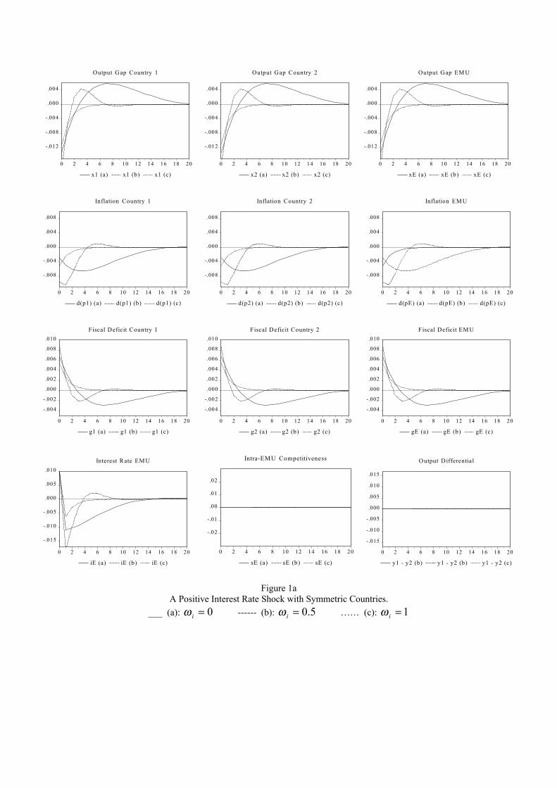
(i) A monetary shock.
This first example studies the effects of a temporary positive shock of 1% to the common interest rate.
The common interest rate is shocked by 1% during period 0 (the interest rate rule is turned off during
period 0). In a monetary union, an interest rate shock is by definition a common, or symmetric shock.
Three alternative regimes are distinguished: regime (a) (solid lines in the graphs) assumes backward-
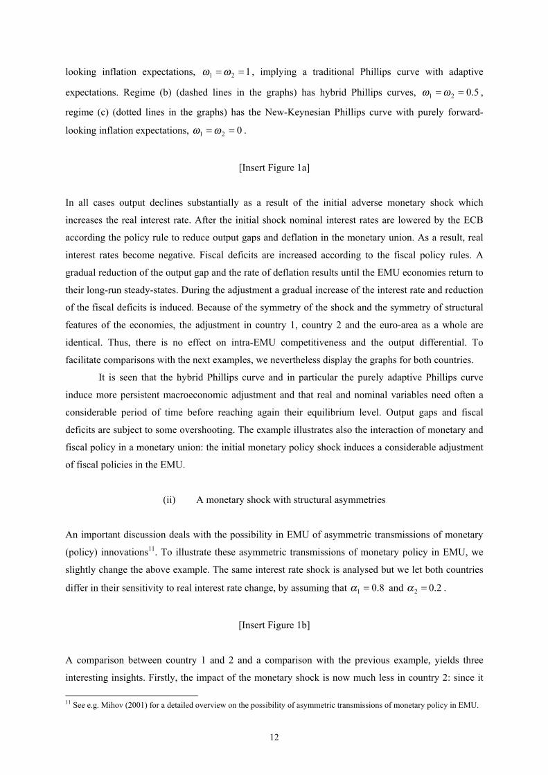
12
looking inflation expectations, 121 == ωω , implying a traditional Phillips curve with adaptive
expectations. Regime (b) (dashed lines in the graphs) has hybrid Phillips curves, 5.021 == ωω ,
regime (c) (dotted lines in the graphs) has the New-Keynesian Phillips curve with purely forward-
looking inflation expectations, 021 == ωω .
[Insert Figure 1a]
In all cases output declines substantially as a result of the initial adverse monetary shock which
increases the real interest rate. After the initial shock nominal interest rates are lowered by the ECB
according the policy rule to reduce output gaps and deflation in the monetary union. As a result, real
interest rates become negative. Fiscal deficits are increased according to the fiscal policy rules. A
gradual reduction of the output gap and the rate of deflation results until the EMU economies return to
their long-run steady-states. During the adjustment a gradual increase of the interest rate and reduction
of the fiscal deficits is induced. Because of the symmetry of the shock and the symmetry of structural
features of the economies, the adjustment in country 1, country 2 and the euro-area as a whole are
identical. Thus, there is no effect on intra-EMU competitiveness and the output differential. To
facilitate comparisons with the next examples, we nevertheless display the graphs for both countries.
It is seen that the hybrid Phillips curve and in particular the purely adaptive Phillips curve
induce more persistent macroeconomic adjustment and that real and nominal variables need often a
considerable period of time before reaching again their equilibrium level. Output gaps and fiscal
deficits are subject to some overshooting. The example illustrates also the interaction of monetary and
fiscal policy in a monetary union: the initial monetary policy shock induces a considerable adjustment
of fiscal policies in the EMU.
(ii) A monetary shock with structural asymmetries
An important discussion deals with the possibility in EMU of asymmetric transmissions of monetary
(policy) innovations11. To illustrate these asymmetric transmissions of monetary policy in EMU, we
slightly change the above example. The same interest rate shock is analysed but we let both countries
differ in their sensitivity to real interest rate change, by assuming that 8.01 =α and 2.02 =α .
[Insert Figure 1b]
A comparison between country 1 and 2 and a comparison with the previous example, yields three
interesting insights. Firstly, the impact of the monetary shock is now much less in country 2: since it
11 See e.g. Mihov (2001) for a detailed overview on the possibility of asymmetric transmissions of monetary policy in EMU.
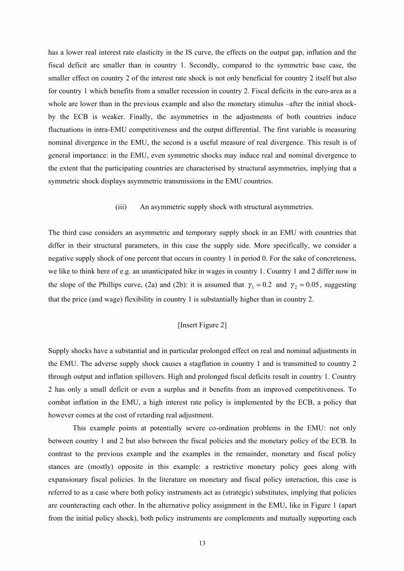
13
has a lower real interest rate elasticity in the IS curve, the effects on the output gap, inflation and the
fiscal deficit are smaller than in country 1. Secondly, compared to the symmetric base case, the
smaller effect on country 2 of the interest rate shock is not only beneficial for country 2 itself but also
for country 1 which benefits from a smaller recession in country 2. Fiscal deficits in the euro-area as a
whole are lower than in the previous example and also the monetary stimulus –after the initial shock-
by the ECB is weaker. Finally, the asymmetries in the adjustments of both countries induce
fluctuations in intra-EMU competitiveness and the output differential. The first variable is measuring
nominal divergence in the EMU, the second is a useful measure of real divergence. This result is of
general importance: in the EMU, even symmetric shocks may induce real and nominal divergence to
the extent that the participating countries are characterised by structural asymmetries, implying that a
symmetric shock displays asymmetric transmissions in the EMU countries.
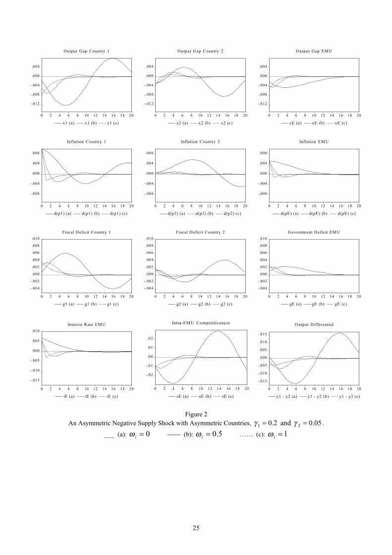
(iii) An asymmetric supply shock with structural asymmetries.
The third case considers an asymmetric and temporary supply shock in an EMU with countries that
differ in their structural parameters, in this case the supply side. More specifically, we consider a
negative supply shock of one percent that occurs in country 1 in period 0. For the sake of concreteness,
we like to think here of e.g. an unanticipated hike in wages in country 1. Country 1 and 2 differ now in
the slope of the Phillips curve, (2a) and (2b): it is assumed that 2.01 =γ and 05.02 =γ , suggesting
that the price (and wage) flexibility in country 1 is substantially higher than in country 2.
[Insert Figure 2]
Supply shocks have a substantial and in particular prolonged effect on real and nominal adjustments in
the EMU. The adverse supply shock causes a stagflation in country 1 and is transmitted to country 2
through output and inflation spillovers. High and prolonged fiscal deficits result in country 1. Country
2 has only a small deficit or even a surplus and it benefits from an improved competitiveness. To
combat inflation in the EMU, a high interest rate policy is implemented by the ECB, a policy that
however comes at the cost of retarding real adjustment.
This example points at potentially severe co-ordination problems in the EMU: not only
between country 1 and 2 but also between the fiscal policies and the monetary policy of the ECB. In
contrast to the previous example and the examples in the remainder, monetary and fiscal policy
stances are (mostly) opposite in this example: a restrictive monetary policy goes along with
expansionary fiscal policies. In the literature on monetary and fiscal policy interaction, this case is
referred to as a case where both policy instruments act as (strategic) substitutes, implying that policies
are counteracting each other. In the alternative policy assignment in the EMU, like in Figure 1 (apart
from the initial policy shock), both policy instruments are complements and mutually supporting each
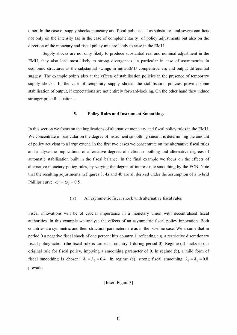
14
other. In the case of supply shocks monetary and fiscal policies act as substitutes and severe conflicts
not only on the intensity (as in the case of complementarity) of policy adjustments but also on the
direction of the monetary and fiscal policy mix are likely to arise in the EMU.
Supply shocks are not only likely to produce substantial real and nominal adjustment in the
EMU, they also lead most likely to strong divergences, in particular in case of asymmetries in
economic structures as the substantial swings in intra-EMU competitiveness and output differential
suggest. The example points also at the effects of stabilisation policies in the presence of temporary
supply shocks. In the case of temporary supply shocks the stabilisation policies provide some
stabilisation of output, if expectations are not entirely forward-looking. On the other hand they induce
stronger price fluctuations.
5. Policy Rules and Instrument Smoothing.
In this section we focus on the implications of alternative monetary and fiscal policy rules in the EMU.
We concentrate in particular on the degree of instrument smoothing since it is determining the amount
of policy activism to a large extent. In the first two cases we concentrate on the alternative fiscal rules
and analyse the implications of alternative degrees of deficit smoothing and alternative degrees of
automatic stabilisation built in the fiscal balance. In the final example we focus on the effects of
alternative monetary policy rules, by varying the degree of interest rate smoothing by the ECB. Note
that the resulting adjustments in Figures 3, 4a and 4b are all derived under the assumption of a hybrid
Phillips curve, 5.021 == ωω .
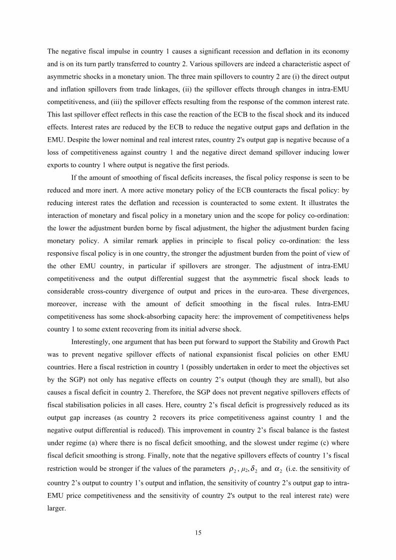
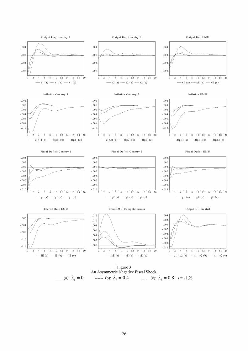
(iv) An asymmetric fiscal shock with alternative fiscal rules
Fiscal innovations will be of crucial importance in a monetary union with decentralised fiscal
authorities. In this example we analyse the effects of an asymmetric fiscal policy innovation. Both
countries are symmetric and their structural parameters are as in the baseline case. We assume that in
period 0 a negative fiscal shock of one percent hits country 1, reflecting e.g. a restrictive discretionary
fiscal policy action (the fiscal rule is turned in country 1 during period 0). Regime (a) sticks to our
original rule for fiscal policy, implying a smoothing parameter of 0. In regime (b), a mild form of
fiscal smoothing is chosen: 4.021 == λλ , in regime (c), strong fiscal smoothing 8.021 == λλ
prevails.
[Insert Figure 3]
15
The negative fiscal impulse in country 1 causes a significant recession and deflation in its economy
and is on its turn partly transferred to country 2. Various spillovers are indeed a characteristic aspect of
asymmetric shocks in a monetary union. The three main spillovers to country 2 are (i) the direct output
and inflation spillovers from trade linkages, (ii) the spillover effects through changes in intra-EMU
competitiveness, and (iii) the spillover effects resulting from the response of the common interest rate.
This last spillover effect reflects in this case the reaction of the ECB to the fiscal shock and its induced
effects. Interest rates are reduced by the ECB to reduce the negative output gaps and deflation in the
EMU. Despite the lower nominal and real interest rates, country 2's output gap is negative because of a
loss of competitiveness against country 1 and the negative direct demand spillover inducing lower
exports to country 1 where output is negative the first periods.
If the amount of smoothing of fiscal deficits increases, the fiscal policy response is seen to be
reduced and more inert. A more active monetary policy of the ECB counteracts the fiscal policy: by
reducing interest rates the deflation and recession is counteracted to some extent. It illustrates the
interaction of monetary and fiscal policy in a monetary union and the scope for policy co-ordination:
the lower the adjustment burden borne by fiscal adjustment, the higher the adjustment burden facing
monetary policy. A similar remark applies in principle to fiscal policy co-ordination: the less
responsive fiscal policy is in one country, the stronger the adjustment burden from the point of view of
the other EMU country, in particular if spillovers are stronger. The adjustment of intra-EMU
competitiveness and the output differential suggest that the asymmetric fiscal shock leads to
considerable cross-country divergence of output and prices in the euro-area. These divergences,
moreover, increase with the amount of deficit smoothing in the fiscal rules. Intra-EMU
competitiveness has some shock-absorbing capacity here: the improvement of competitiveness helps
country 1 to some extent recovering from its initial adverse shock.
Interestingly, one argument that has been put forward to support the Stability and Growth Pact
was to prevent negative spillover effects of national expansionist fiscal policies on other EMU
countries. Here a fiscal restriction in country 1 (possibly undertaken in order to meet the objectives set
by the SGP) not only has negative effects on country 2’s output (though they are small), but also
causes a fiscal deficit in country 2. Therefore, the SGP does not prevent negative spillovers effects of
fiscal stabilisation policies in all cases. Here, country 2’s fiscal deficit is progressively reduced as its
output gap increases (as country 2 recovers its price competitiveness against country 1 and the
negative output differential is reduced). This improvement in country 2’s fiscal balance is the fastest
under regime (a) where there is no fiscal deficit smoothing, and the slowest under regime (c) where
fiscal deficit smoothing is strong. Finally, note that the negative spillovers effects of country 1’s fiscal
restriction would be stronger if the values of the parameters 2ρ , μ2, 2δ and 2α (i.e. the sensitivity of
country 2’s output to country 1’s output and inflation, the sensitivity of country 2’s output gap to intra-
EMU price competitiveness and the sensitivity of country 2's output to the real interest rate) were
larger.
16
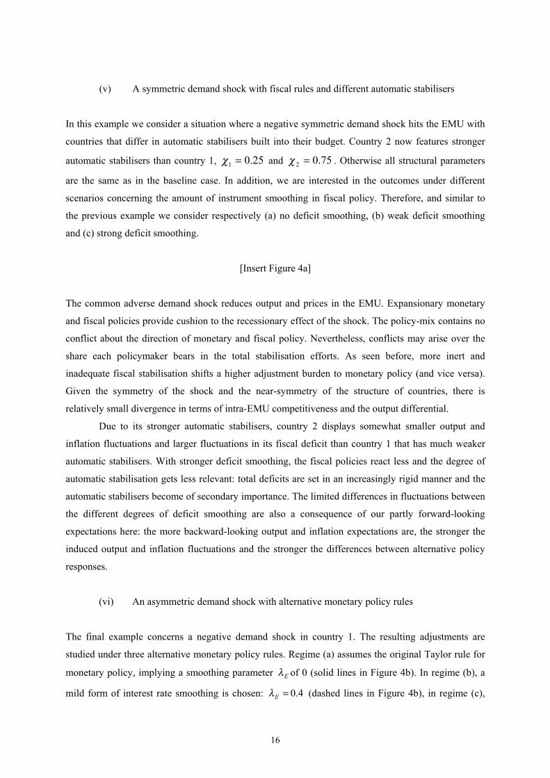
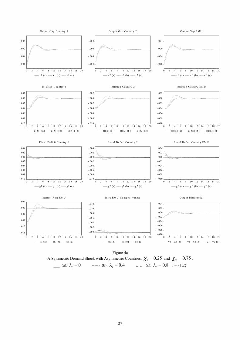
(v) A symmetric demand shock with fiscal rules and different automatic stabilisers
In this example we consider a situation where a negative symmetric demand shock hits the EMU with
countries that differ in automatic stabilisers built into their budget. Country 2 now features stronger
automatic stabilisers than country 1, 25.01 =χ and 75.02 =χ . Otherwise all structural parameters
are the same as in the baseline case. In addition, we are interested in the outcomes under different
scenarios concerning the amount of instrument smoothing in fiscal policy. Therefore, and similar to
the previous example we consider respectively (a) no deficit smoothing, (b) weak deficit smoothing
and (c) strong deficit smoothing.
[Insert Figure 4a]
The common adverse demand shock reduces output and prices in the EMU. Expansionary monetary
and fiscal policies provide cushion to the recessionary effect of the shock. The policy-mix contains no
conflict about the direction of monetary and fiscal policy. Nevertheless, conflicts may arise over the
share each policymaker bears in the total stabilisation efforts. As seen before, more inert and
inadequate fiscal stabilisation shifts a higher adjustment burden to monetary policy (and vice versa).
Given the symmetry of the shock and the near-symmetry of the structure of countries, there is
relatively small divergence in terms of intra-EMU competitiveness and the output differential.
Due to its stronger automatic stabilisers, country 2 displays somewhat smaller output and
inflation fluctuations and larger fluctuations in its fiscal deficit than country 1 that has much weaker
automatic stabilisers. With stronger deficit smoothing, the fiscal policies react less and the degree of
automatic stabilisation gets less relevant: total deficits are set in an increasingly rigid manner and the
automatic stabilisers become of secondary importance. The limited differences in fluctuations between
the different degrees of deficit smoothing are also a consequence of our partly forward-looking
expectations here: the more backward-looking output and inflation expectations are, the stronger the
induced output and inflation fluctuations and the stronger the differences between alternative policy
responses.
(vi) An asymmetric demand shock with alternative monetary policy rules
The final example concerns a negative demand shock in country 1. The resulting adjustments are
studied under three alternative monetary policy rules. Regime (a) assumes the original Taylor rule for
monetary policy, implying a smoothing parameter Eλ of 0 (solid lines in Figure 4b). In regime (b), a
mild form of interest rate smoothing is chosen: 4.0=Eλ (dashed lines in Figure 4b), in regime (c),
17
strong interest rate smoothing 8.0=Eλ prevails (dotted lines in Figure 4b). Fiscal policy rules are
again set at their baseline setting without deficit smoothing.
[Insert Figure 4b]
In much of the discussion on EMU, asymmetric shocks have been focused upon, since in that case the
loss of monetary policy and exchange rate flexibility may be the most problematic, in particular if also
fiscal policy is restricted. Some of these fears are confirmed in our example: country 1 experiences a
substantial output gap and adjustment burden. Part of the adjustment is also shared by country 2 as its
exports to country 1 are reduced, lowering output in country 2 as well. Clearly visible is also that more
flexibility of monetary policy, i.e. less interest rate smoothing, reduces the adjustment problems to
some extent. It puts also off some pressure on fiscal policies: with less interest rate smoothing, the
fiscal deficit adjustment reduces since the fluctuations in output are more actively counteracted by the
ECB already. In this case, countries are symmetric in their economic structure and we see that the
different degrees of interest rate smoothing have no differential effect on the nominal and real
divergence as adjustments of intra-EMU competitiveness and the output differential are the same
across the interest rate rules.
6. Efficiency of Policy Rules in EMU.
In the literature on policy rules the efficiency and robustness of alternative policy rules is often
investigated, see e.g. Taylor (1999b). The relative efficiency of policy rules can be assessed by
carrying out stochastic simulations and comparing the resulting standard deviations of inflation, output
gaps and instrument variables under alternative rules. Robustness of policy rules can be assessed by
comparing the performance of the same rule under different parameter settings of the model -like we
have done to some extent in our examples- or the performance of the same rule across different
models -something which is beyond the scope of the present analysis-.
To assess the efficiency of the policy rules, we carried out stochastic simulations of the
examples (iii)-(v) analysed in the previous section, i.e. the respective shocks in these examples are
repeated 100 times and the resulting standard deviations calculated. Efficiency is measured here by
weighting inflation, output and instrument variability in the following manner:
)()()()( 111111 gVarxVarVarLE φβπ ++= (5a)
)()()()( 222222 gVarxVarVarLE φβπ ++= (5b)
)()()()( EEEEEE iVarxVarVarLE φβπ ++= (5b)
18
We assume that inflation and output variability are equally weighted, i.e. 1=iβ , whereas instrument
variability carries halve the weight of output and inflation variability, i.e. 5.0=iφ , in calculating
expected losses. The variability of a variable is measured by its variance (Var) and its standard
deviation (Std). Table 2 gives the standard deviation of inflation rates, output gaps, the interest rate
and fiscal deficits in the examples above and the resulting expected losses:
Table 2
Efficiency of Alternative Macroeconomic Policy Rules
Std(π1) Std(π2) Std(πE) Std(x1) Std(x2) Std(xE) Std(iE) Std(g1) Std(g2) E(L1) E(L2) E(LE)
iii (a) 0.00683 0.00425 0.00550 0.01174 0.00136 0.00658 0.01070 0.01371 0.00041 0.02543 0.00582 0.01743
iii (b) 0.01280 0.00818 0.01053 0.01665 0.00228 0.00935 0.01901 0.01590 0.00062 0.0374 0.01077 0.02939
iii (c) 0.02860 0.01863 0.02281 0.02411 0.00697 0.01371 0.03799 0.01959 0.00337 0.06251 0.02729 0.05552
iv (a) 0.01067 0.00985 0.00990 0.01732 0.01328 0.01217 0.01944 0.00433 0.00466 0.03016 0.02546 0.03179
iv (b) 0.00972 0.00912 0.00920 0.01639 0.01464 0.01338 0.01917 0.00281 0.00357 0.02752 0.02555 0.03217
iv (c) 0.01033 0.00891 0.00925 0.01948 0.01684 0.01528 0.02067 0.00145 0.00227 0.03054 0.02689 0.03487
v (a) 0.00843 0.00525 0.00679 0.01448 0.00168 0.00813 0.01320 0.00724 0.00084 0.02653 0.00735 0.02152
v (b) 0.00698 0.00354 0.00525 0.01471 0.00365 0.00916 0.00906 0.00735 0.00183 0.02537 0.00811 0.01894
v (c) 0.00794 0.00518 0.00622 0.01884 0.00810 0.01316 0.00396 0.00942 0.00405 0.03149 0.01531 0.02136
Note: displayed are standard deviations of inflation rates, output gaps and instrument variables of stochasticsimulations of examples iii, iv, v. (a), (b) and (c) denote the policy regimes -defined in terms of instrumentsmoothing- in place, see also the analysis before. Welfare losses are calculated according to (5).
In the above examples a higher degree of instrument smoothing is generally inefficient in
terms of stabilising output and inflation, since it reduces the necessary instrument adjustment to
macroeconomic shocks. Example (iii) shows that instrument smoothing also does not reduce by
definition instrument variability as the policy instruments often have to be used for longer periods than
in cases with less instrument smoothing due to the slow adjustment in the first periods after the shocks
have incurred. Nevertheless, instrument variability is lower with higher smoothing in the case of fiscal
policy in example (iv) and in case of monetary policy in example (v). The non-smoothing fiscal policy
rule is efficient for all three authorities in case (iii) and for country 2 and the ECB also in case (v) with
asymmetric shocks to country 1. In the case of example (iv) and (v) the mild smoothing case would be
more efficient for country 1 and the ECB.
As noted before, however, institutional restrictions may require instrumental smoothing. In the
context of EMU, we also note that the provisions of the SGP may limit the flexibility of fiscal policy
in the short run if countries face a negative shock and less room for manoeuvrability e.g. due to the
presence of strong automatic stabilisers. In such a situation, fiscal authorities may be forced, while not
optimal, to follow a fiscal policy rule with strong deficit smoothing. Sack and Wieland (2000) show
that instrument smoothing may become less inefficient with (i) entirely forward-looking market
19
participants, (ii) measurement error with key macroeconomic variables and (iii) uncertainty regarding
relevant structural parameters. In such conditions more cautious policymaking may become efficient.
7. Conclusions.
Recent macroeconomic research has focused on the working and effects of macroeconomic policy
rules. This paper has applied the insights of the recent new-Keynesian literature on monetary as well
as fiscal policy rules to the EMU case. Using a stylised two-country model of the EMU, we have
shown by means of simulations that insights as to effectiveness and efficiency of macroeconomic
policy can be obtained from a “policy-rules” based approach to monetary and fiscal policy design in
the EMU. The EMU is an interesting case because it combines monetary policy designed at the supra-
national (federal) level with fiscal policy chosen at the national level but subject to restrictions in the
form of the SGP. Using numerical simulations, we specifically have analysed how three aspects play a
crucial role in our model (i) the design of monetary and fiscal policy rules themselves, (ii)
asymmetries between EMU countries in terms of macroeconomic shocks and macroeconomic
structures-, (iii) the degree of backward and forward-looking behaviour in consumer decisions and
inflation expectations.
20
References
Aksoy, Y., P. de Grauwe, and H. Dewachter (2002), Do Asymmetries Matter for European MonetaryPolicy, European Economic Review, vol.46, 443-469.
Artis, M. and B. Winkler (1997), The Stability Pact: Safeguarding the Credibility of the EuropeanCentral Bank. CEPR Discussion Paper, no. 1688.
Ballabriga, F. and C. Martinez-Mongay (2002), Has EMU Shifted Policy?, Economic Papers no.166,European Commission.
Batini, N. and A. Haldane (1999), Forward-Looking Rules for Monetary Policy, in J. Taylor (1999a),Monetary Policy Rules, NBER Studies in Business Cycles, vol. 31, 157-92.
Benhabib, J., S. Schmitt-Grohé and M. Uribe (2001), Monetary Policy and Multiple Equilibria,American Economic Review, vol.91(1), 167-185.
Buti, M., D. Franco and H. Ongena (1997), Budgetary Policies during Recessions – RetrospectiveApplication of the “Stability and Growth Pact” to the Post-War Period, Recherches Économiques deLouvain, vol.63(4), 321-66.
Buti, M, W. Roeger and J. in ‘t Veld (2001), Stabilising Output and Inflation in EMU: Policy Conflictsand Co-operation under the Stability Pact, mimeo.
Buti, M., and A. Sapir (1998), Economic Policy in EMU – A Study by the European CommissionServices, Oxford University Press.
Clarida, R., J. Gali, and M. Gertler (1999), The Science of Monetary Policy: A New KeynesianPerspective, Journal of Economic Literature, vol.37, 1661-1707.
Clarida, R. J. Gali, and M. Gertler (2002), A Simple Framework for International Monetary PolicyAnalysis, CEPR Discussion Paper no.3555.
Dieppe, A. and J. Henry (2002), The Euro Area Viewed as a Single Economy: How Does it Respondto Shocks?, mimeo.
Equipe MIMOSA (1996), La nouvelle version de MIMOSA, modèle de l’économie mondiale, Revuede l’OFCE, No. 58, Juillet, 103-55.
European Central Bank (2003), The Relationship between Monetary Policy and Fiscal Policies in theEuro Area, Monthly Bulletin February.
European Commission (2000), Public Finances in EMU – 2000, European Economy, No. 3.
European Commission (2001), Public Finances in EMU − 2001, European Economy, No. 3.
European Commission (2002), Public Finances in EMU − 2002, European Economy, No. 3.
Evans, G. and S. Honkapohja (2002), Monetary Policy, Expectations and Commitment, CEPRDiscussion Paper 3434.
Fase, M. (2001), Monetary Policy Rules for EMU, De Nederlandsche Bank Reprint 731.
21
Fisher, P. (1982), Rational Expectations in Macroeconomic Models, Dordrecht: Kluwer AcademicPublishers.
Fuhrer, J. and G. Moore (1995), Monetary Policy Trade-Offs and the Correlation between NominalInterest Rates and Real Output, American Economic Review, vol.85(1), 219-239.
Gagnon, J. and J. Ihrig (2002), Monetary Policy and Exchange Rate Pass-Through, InternationalFinance Discussion Papers No.704, Board of Governors of the Federal Reserve System
Gali, J. and T. Monacelli (2002), Monetary Policy and Exchange Rate Volatility in a Small OpenEconomy, CEPR Discussion Paper no.3346.
Gerlach, S. and G. Schnabel (2000), The Taylor Rule and Interest Rates in the EMU Area, EconomicsLetters, vol.67, 165-171.
Gerlach, S. and F. Smets (1999), Output Gaps and Monetary Policy in the EMU Area, EuropeanEconomic Review, vol.43, 801-812.
Huh, C. and K. Lansing (2000), Expectations, Credibility, and Disinflation in a Small MacroeconomicModel, Journal of Economics and Business, vol.51(1-2), 51-86.
Hunt, B. and D. Laxton (2002), Some Simulation Properties of the Major Euro Area Economies inMULTIMOD, mimeo.
Leeper, E. (1991), Equilibria under 'Active' and 'Passive' Monetary and Fiscal Policies, Journal ofMonetary Economics, vol.27, 129-147.
Leeper, E. and T. Zha (2000), Assessing Simple Policy Rules: A View from a Complete MacroModel, Federal Reserve Bank of Atlanta Working Paper 2000-19.
Leith, C. and J. Malley (2002), Estimated General Equilibrium Models for the Evaluation of MonetaryPolicy in the US and Europe, CESifo Working Paper no.699.
Leith, C. and S. Wren-Lewis (2000), Interactions between Monetary and Fiscal Policy Rules,Economic Journal, vol. 110, C93-108.
Leith, C. and S. Wren-Lewis (2001), Interest Rate Feedback Rules in an Open Economy with ForwardLooking Inflation, Oxford Bulletin of Economics and Statistics, vol. 63(2), 209-31.
Levin A., V. Wieland and J. Williams (1999), Robustness of Simple Monetary Policy Rules underModel Uncertainty, in J. Taylor ed., Monetary Policy Rules, NBER Studies in Business Cycles, vol.31, Chicago: University of Chicago Press, 263-99.
McCallum, B. T. (2001), Should Monetary Policy Respond Strongly to Output Gaps, AEA Papers andProceedings, vol. 91(2), 258-62.
McCallum, B. and E. Nelson (1999a), Nominal Income Targeting in an Open-Economy OptimizingModel, Journal of Monetary Economics, vol.43, 553-78.
McCallum, B. and E. Nelson (1999b), Performance of Operational Policy Rules in an EstimatedSemiclassical Structural Model, in J. Taylor ed., Monetary Policy Rules, NBER Studies in BusinessCycles, Vol. 31, Chicago: University of Chicago Press, 15-56.
Mihov, I. (2001), One Monetary Policy in EMU, Economic Policy, vol.33, 369-406.
22
Mitchell, P., J. Sault and K. Wallis (2000), Fiscal Policy Rules in Macroeconomic Models: Principlesand Practice, Economic Modelling, vol.17, 171-93.
van den Noord, P. (2000), The Size and Role of Automatic Fiscal Stabilisers in the 1990s and Beyond,OECD Economics Department Working Papers, no. 230.
Roeger, W. and J. in 't Veld (2002), Some Selected Simulation Experiments with the EuropeanCommission's QUEST Model, mimeo.
Rotemberg, J. and Woodford M. (1999), Interest Rate Rules in an Estimated Sticky Price Model, in J.Taylor ed., Monetary Policy Rules, NBER Studies in Business Cycles, vol. 31, Chicago: University ofChicago Press, 57-119.
Rudebusch, G. and L. Svensson (1999), Policy Rules for Inflation Targeting, in J. Taylor ed.,Monetary Policy Rules, NBER Business Cycles Series, vol.31. Chicago: University of Chicago Press,203-246.
Rudebusch, G. (2002), Assessing Nominal Income Rules for Monetary Policy with Model and DataUncertainty, Economic Journal, vol.112, 402-432.
Sack, B. and V. Wieland (2000), Interest-Rate Smoothing and Optimal Monetary Policy: A Review ofRecent Empirical Evidence, Journal of Economics and Business, vol.52(1-2), 205-228.
Taylor, J. (1993a), Discretion Versus Policy Rules in Practice, Carnegie-Rochester Conference Serieson Public Policy, vol.39, 195-214.
Taylor, J. (1993b), Macroeconomic Policy in a World Economy: From Econometric Design toPractical Operation. New York: W. W. Norton.
Taylor, J. (1994), The Inflation/Output Variability Trade-Off Revisited, in J. Fuhrer (ed.) Goals,Guidelines and Constraints Facing Monetary Policymakers, Federal Reserve Bank of Boston.
Taylor, J. (1999a), A Historical Analysis of Monetary Policy Rules, in J. Taylor ed., Monetary PolicyRules, NBER Business Cycles Series, vol.31. Chicago: University of Chicago Press, 319-341.
Taylor, J. (1999b), The Robustness and Efficiency of Monetary Policy Rules as Guidelines for InterestRate Setting by the European Central Bank, Journal of Monetary Economics, vol.43(3), 655-679.
Taylor, J. (2000), Reassessing Discretionary Fiscal Policy, Journal of Economic Perspectives,vol.14(3), 21-36.
Taylor, J. (2001), The Role of the Exchange Rate in Monetary-Policy Rules, AEA Papers andProceedings, vol. 91(2), May, 263-267.
Woodford, M. (2001), The Taylor Rule and Optimal Monetary Policy, American Economic Review,vol.91(2), 232-237
-.012
-.008
-.004
.000
.004
0 2 4 6 8 10 12 14 16 18 20
x1 (a) x1 (b) x1 (c)
Output Gap Country 1
-.012
-.008
-.004
.000
.004
0 2 4 6 8 10 12 14 16 18 20
x2 (a) x2 (b) x2 (c)
Output Gap Country 2
-.012
-.008
-.004
.000
.004
0 2 4 6 8 10 12 14 16 18 20
xE (a) xE (b) xE (c)
Output Gap EM U
-.008
-.004
.000
.004
.008
0 2 4 6 8 10 12 14 16 18 20
d(p1) (a) d(p1) (b) d(p1) (c)
Inflation Country 1
-.008
-.004
.000
.004
.008
0 2 4 6 8 10 12 14 16 18 20
d(p2) (a) d(p2) (b) d(p2) (c)
Inflation Country 2
-.008
-.004
.000
.004
.008
0 2 4 6 8 10 12 14 16 18 20
d(pE) (a) d(pE) (b) d(pE) (c)
Inflation EM U
-.004
-.002
.000
.002
.004
.006
.008
.010
0 2 4 6 8 10 12 14 16 18 20
g1 (a) g1 (b) g1 (c)
Fiscal Deficit Country 1
-.004
-.002
.000
.002
.004
.006
.008
.010
0 2 4 6 8 10 12 14 16 18 20
g2 (a) g2 (b) g2 (c)
Fiscal Deficit Country 2
-.004
-.002
.000
.002
.004
.006
.008
.010
0 2 4 6 8 10 12 14 16 18 20
gE (a) gE (b) gE (c)
Fiscal Deficit EM U
-.015
-.010
-.005
.000
.005
.010
0 2 4 6 8 10 12 14 16 18 20
iE (a) iE (b) iE (c)
Interest Rate EM U
-.02
-.01
.00
.01
.02
0 2 4 6 8 10 12 14 16 18 20
sE (a) sE (b) sE (c)
Intra-EM U Competitiveness
-.015
-.010
-.005
.000
.005
.010
.015
0 2 4 6 8 10 12 14 16 18 20
y1 - y2 (b) y1 - y2 (b) y1 - y2 (c)
Output Differential
Figure 1aA Positive Interest Rate Shock with Symmetric Countries.
___ (a): 0=iω ------ (b): 5.0=iω …… (c): 1=iω

24
-.012
-.008
-.004
.000
.004
0 2 4 6 8 10 12 14 16 18 20
x1 (a) x1 (b) x1 (c)
Output Gap Country 1
-.012
-.008
-.004
.000
.004
0 2 4 6 8 10 12 14 16 18 20
x2 (a) x2 (b) x2 (c)
Output Gap Country 2
-.012
-.008
-.004
.000
.004
0 2 4 6 8 10 12 14 16 18 20
xE (a) xE (b) xE (c)
Output Gap EM U
-.008
-.004
.000
.004
.008
0 2 4 6 8 10 12 14 16 18 20
d(p1) (a) d(p1) (b) d(p1) (c)
Inflation Country 1
-.008
-.004
.000
.004
.008
0 2 4 6 8 10 12 14 16 18 20
d(p2) (a) d(p2) (b) d(p2) (c)
Inflation Country 2
-.008
-.004
.000
.004
.008
0 2 4 6 8 10 12 14 16 18 20
d(pE) (a) d(pE) (b) d(pE) (c)
Inflation EM U
-.004
-.002
.000
.002
.004
.006
.008
.010
0 2 4 6 8 10 12 14 16 18 20
g1 (a) g1 (b) g1 (c)
Fiscal Deficit Country 1
-.004
-.002
.000
.002
.004
.006
.008
.010
0 2 4 6 8 10 12 14 16 18 20
g2 (a) g2 (b) g2 (c)
Fiscal Deficit Country 2
-.004
-.002
.000
.002
.004
.006
.008
.010
0 2 4 6 8 10 12 14 16 18 20
gE (a) gE (b) gE (c)
Fiscal Deficit EM U
-.015
-.010
-.005
.000
.005
.010
0 2 4 6 8 10 12 14 16 18 20
iE (a) iE (b) iE (c)
Interest Rate EM U
-.02
-.01
.00
.01
.02
0 2 4 6 8 10 12 14 16 18 20
sE (a) sE (b) sE (c)
Intra-EM U Competitiveness
-.015
-.010
-.005
.000
.005
.010
.015
0 2 4 6 8 10 12 14 16 18 20
y1 - y2 (a) y1 - y2 (b) y1 - y2 (c)
Output Differential
Figure 1bA Positive Interest Rate Shock with Asymmetric Countries, 8.01 =α and 2.02 =α .
___ (a): 0=iω ------ (b): 5.0=iω …… (c): 1=iω
25
-.012
-.008
-.004
.000
.004
0 2 4 6 8 10 12 14 16 18 20
x1 (a) x1 (b) x1 (c)
Output Gap Country 1
-.012
-.008
-.004
.000
.004
0 2 4 6 8 10 12 14 16 18 20
x2 (a) x2 (b) x2 (c)
Output Gap Country 2
-.012
-.008
-.004
.000
.004
0 2 4 6 8 10 12 14 16 18 20
xE (a) xE (b) xE (c)
Output Gap EM U
-.008
-.004
.000
.004
.008
0 2 4 6 8 10 12 14 16 18 20
d(p1) (a) d(p1) (b) d(p1) (c)
Inflation Country 1
-.008
-.004
.000
.004
.008
0 2 4 6 8 10 12 14 16 18 20
d(p2) (a) d(p2) (b) d(p2) (c)
Inflation Country 2
-.008
-.004
.000
.004
.008
0 2 4 6 8 10 12 14 16 18 20
d(pE) (a) d(pE) (b) d(pE) (c)
Inflation EM U
-.004
-.002
.000
.002
.004
.006
.008
.010
0 2 4 6 8 10 12 14 16 18 20
g1 (a) g1 (b) g1 (c)
Fiscal Deficit Country 1
-.004
-.002
.000
.002
.004
.006
.008
.010
0 2 4 6 8 10 12 14 16 18 20
g2 (a) g2 (b) g2 (c)
Fiscal Deficit Country 2
-.004
-.002
.000
.002
.004
.006
.008
.010
0 2 4 6 8 10 12 14 16 18 20
gE (a) gE (b) gE (c)
Government Deficit EM U
-.015
-.010
-.005
.000
.005
.010
0 2 4 6 8 10 12 14 16 18 20
iE (a) iE (b) iE (c)
Interest Rate EM U
-.02
-.01
.00
.01
.02
0 2 4 6 8 10 12 14 16 18 20
sE (a) sE (b) sE (c)
Intra-EM U Competitiveness
-.015
-.010
-.005
.000
.005
.010
.015
0 2 4 6 8 10 12 14 16 18 20
y1 - y2 (a) y1 - y2 (b) y1 - y2 (c)
Output Differential
Figure 2An Asymmetric Negative Supply Shock with Asymmetric Countries, 2.01 =γ and 05.02 =γ .
___ (a): 0=iω ------ (b): 5.0=iω …… (c): 1=iω
26
-.008
-.004
.000
.004
0 2 4 6 8 10 12 14 16 18 20
x1 (a) x1 (b) x1 (c)
Output Gap Country 1
-.008
-.004
.000
.004
0 2 4 6 8 10 12 14 16 18 20
x2 (a) x2 (b) x2 (c)
Output Gap Country 2
-.008
-.004
.000
.004
0 2 4 6 8 10 12 14 16 18 20
xE (a) xE (b) xE (c)
Output Gap EM U
-.010
-.008
-.006
-.004
-.002
.000
.002
0 2 4 6 8 10 12 14 16 18 20
d(p1) (a) d(p1) (b) d(p1) (c)
Inflation Country 1
-.010
-.008
-.006
-.004
-.002
.000
.002
0 2 4 6 8 10 12 14 16 18 20
d(p2) (a) d(p2) (b) d(p2) (c)
Inflation Country 2
-.010
-.008
-.006
-.004
-.002
.000
.002
0 2 4 6 8 10 12 14 16 18 20
d(pE) (a) d(pE) (b) d(pE) (c)
Inflation EM U
-.010
-.008
-.006
-.004
-.002
.000
.002
.004
0 2 4 6 8 10 12 14 16 18 20
g1 (a) g1 (b) g1 (c)
Fiscal Deficit Country 1
-.010
-.008
-.006
-.004
-.002
.000
.002
.004
0 2 4 6 8 10 12 14 16 18 20
g2 (a) g2 (b) g2 (c)
Fiscal Deficit Country 2
-.010
-.008
-.006
-.004
-.002
.000
.002
.004
0 2 4 6 8 10 12 14 16 18 20
gE (a) gE (b) gE (c)
Fiscal Deficit EM U
-.016
-.012
-.008
-.004
.000
0 2 4 6 8 10 12 14 16 18 20
iE (a) iE (b) iE (c)
Interest Rate EMU
.000
.002
.004
.006
.008
.010
.012
0 2 4 6 8 10 12 14 16 18 20
sE (a) sE (b) sE (c)
Intra-EMU Competitiveness
-.010
-.008
-.006
-.004
-.002
.000
.002
.004
0 2 4 6 8 10 12 14 16 18 20
y1 - y2 (a) y1 - y2 (b) y1 - y2 (c)
Output Differential
Figure 3An Asymmetric Negative Fiscal Shock.
___ (a): 0=iλ ------ (b): 4.0=iλ …… (c): 8.0=iλ i = {1,2}
27
-.008
-.004
.000
.004
0 2 4 6 8 10 12 14 16 18 20
x1 (a) x1 (b) x1 (c)
Output Gap Country 1
-.008
-.004
.000
.004
0 2 4 6 8 10 12 14 16 18 20
x2 (a) x2 (b) x2 (c)
Output Gap Country 2
-.008
-.004
.000
.004
0 2 4 6 8 10 12 14 16 18 20
xE (a) xE (b) xE (c)
Output Gap EM U
-.010
-.008
-.006
-.004
-.002
.000
.002
0 2 4 6 8 10 12 14 16 18 20
d(p1) (a) d(p1) (b) d(p1) (c)
Inflation Country 1
-.010
-.008
-.006
-.004
-.002
.000
.002
0 2 4 6 8 10 12 14 16 18 20
d(p2) (a) d(p2) (b) d(p2) (c)
Inflation Country 2
-.010
-.008
-.006
-.004
-.002
.000
.002
0 2 4 6 8 10 12 14 16 18 20
d(pE) (a) d(pE) (b) d(pE) (c)
Inflation Country EM U
-.010
-.008
-.006
-.004
-.002
.000
.002
.004
0 2 4 6 8 10 12 14 16 18 20
g1 (a) g1 (b) g1 (c)
Fiscal Deficit Country 1
-.010
-.008
-.006
-.004
-.002
.000
.002
.004
0 2 4 6 8 10 12 14 16 18 20
g2 (a) g2 (b) g2 (c)
Fiscal Deficit Country 2
-.010
-.008
-.006
-.004
-.002
.000
.002
.004
0 2 4 6 8 10 12 14 16 18 20
gE (a) gE (b) gE (c)
Fiscal Deficit Country EM U
-.016
-.012
-.008
-.004
.000
.004
0 2 4 6 8 10 12 14 16 18 20
iE (a) iE (b) iE (c)
Interest Rate EM U
.000
.002
.004
.006
.008
.010
.012
0 2 4 6 8 10 12 14 16 18 20
sE (a) sE (b) sE (c)
Intra-EM U Competitiveness
-.010
-.008
-.006
-.004
-.002
.000
.002
.004
0 2 4 6 8 10 12 14 16 18 20
y1 - y2 (a) y1 - y2 (b) y1 - y2 (c)
Output Differential
Figure 4aA Symmetric Demand Shock with Asymmetric Countries, 25.01 =χ and 75.02 =χ .
___ (a): 0=iλ ------ (b): 4.0=iλ …… (c): 8.0=iλ i = {1,2}
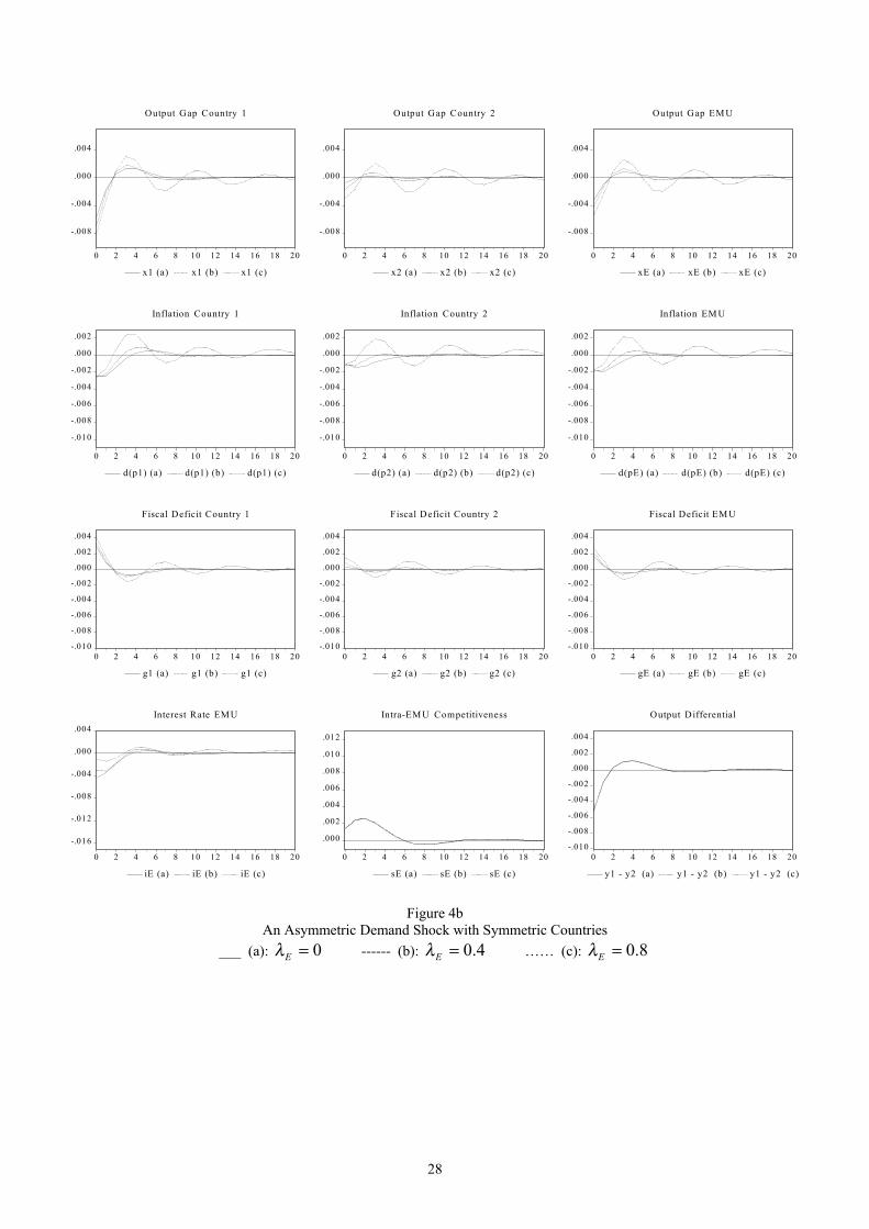
28
-.008
-.004
.000
.004
0 2 4 6 8 10 12 14 16 18 20
x1 (a) x1 (b) x1 (c)
Output Gap Country 1
-.008
-.004
.000
.004
0 2 4 6 8 10 12 14 16 18 20
x2 (a) x2 (b) x2 (c)
Output Gap Country 2
-.008
-.004
.000
.004
0 2 4 6 8 10 12 14 16 18 20
xE (a) xE (b) xE (c)
Output Gap EM U
-.010
-.008
-.006
-.004
-.002
.000
.002
0 2 4 6 8 10 12 14 16 18 20
d(p1) (a) d(p1) (b) d(p1) (c)
Inflation Country 1
-.010
-.008
-.006
-.004
-.002
.000
.002
0 2 4 6 8 10 12 14 16 18 20
d(p2) (a) d(p2) (b) d(p2) (c)
Inflation Country 2
-.010
-.008
-.006
-.004
-.002
.000
.002
0 2 4 6 8 10 12 14 16 18 20
d(pE) (a) d(pE) (b) d(pE) (c)
Inflation EM U
-.010
-.008
-.006
-.004
-.002
.000
.002
.004
0 2 4 6 8 10 12 14 16 18 20
g1 (a) g1 (b) g1 (c)
Fiscal Deficit Country 1
-.010
-.008
-.006
-.004
-.002
.000
.002
.004
0 2 4 6 8 10 12 14 16 18 20
g2 (a) g2 (b) g2 (c)
Fiscal Deficit Country 2
-.010
-.008
-.006
-.004
-.002
.000
.002
.004
0 2 4 6 8 10 12 14 16 18 20
gE (a) gE (b) gE (c)
Fiscal Deficit EM U
-.016
-.012
-.008
-.004
.000
.004
0 2 4 6 8 10 12 14 16 18 20
iE (a) iE (b) iE (c)
Interest Rate EM U
.000
.002
.004
.006
.008
.010
.012
0 2 4 6 8 10 12 14 16 18 20
sE (a) sE (b) sE (c)
Intra-EM U Competitiveness
-.010
-.008
-.006
-.004
-.002
.000
.002
.004
0 2 4 6 8 10 12 14 16 18 20
y1 - y2 (a) y1 - y2 (b) y1 - y2 (c)
Output Differential
Figure 4bAn Asymmetric Demand Shock with Symmetric Countries
___ (a): 0=Eλ ------ (b): 4.0=Eλ …… (c): 8.0=Eλ