Embed Size (px)
Citation preview
The Pennsylvania State University
The Graduate School
Department of Architectural Engineering
ESTABLISHING INVERSE MODELING ANALYSIS TOOLS TO ENABLE
CONTINUOUS EFFICIENCY IMPROVEMENT LOOP IMPLEMENTATION
A Thesis in
Architectural Engineering
by
Mona Hatami
2016 Mona Hatami
Submitted in Partial Fulfillment
of the Requirements
for the Degree of
Master of Science
May 2016

ii
The thesis of Zahra Hatami was reviewed and approved* by the following:
James D. Freihaut
Professor of Architectural Engineering
Thesis Advisor
Stephen Treado
Associate Professor of Architectural Engineering
Ali Memari
Hankin Chair Professor of Architectural Engineering
Chimay J. Anumba
Professor of Architectural Engineering
Head of the Department of Architectural Engineering
*Signatures are on file in the Graduate School
iii
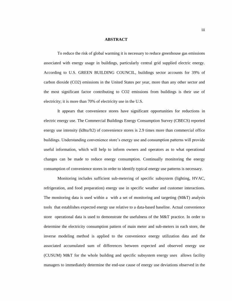
ABSTRACT
To reduce the risk of global warming it is necessary to reduce greenhouse gas emissions
associated with energy usage in buildings, particularly central grid supplied electric energy.
According to U.S. GREEN BUILDING COUNCIL, buildings sector accounts for 39% of
carbon dioxide (CO2) emissions in the United States per year, more than any other sector and
the most significant factor contributing to CO2 emissions from buildings is their use of
electricity; it is more than 70% of electricity use in the U.S.
It appears that convenience stores have significant opportunities for reductions in
electric energy use. The Commercial Buildings Energy Consumption Survey (CBECS) reported
energy use intensity (kBtu/ft2) of convenience stores is 2.9 times more than commercial office
buildings. Understanding convenience store’s energy use and consumption patterns will provide
useful information, which will help to inform owners and operators as to what operational
changes can be made to reduce energy consumption. Continually monitoring the energy
consumption of convenience stores in order to identify typical energy use patterns is necessary.
Monitoring includes sufficient sub-metering of specific subsystem (lighting, HVAC,
refrigeration, and food preparation) energy use in specific weather and customer interactions.
The monitoring data is used within a with a set of monitoring and targeting (M&T) analysis
tools that establishes expected energy use relative to a data-based baseline. Actual convenience
store operational data is used to demonstrate the usefulness of the M&T practice. In order to
determine the electricity consumption pattern of main meter and sub-meters in each store, the
inverse modeling method is applied to the convenience energy utilization data and the
associated accumulated sum of differences between expected and observed energy use
(CUSUM) M&T for the whole building and specific subsystem energy uses allows facility
managers to immediately determine the end-use cause of energy use deviations observed in the

iv
energy use CUSUM reporting. The results indicate that the similarly designed stores exhibit
very similar qualitative energy use dependencies with changes in ambient weather conditions
with respect to whole building energy use and subsystem energy uses. However, the
quantitative levels of energy use as well as the changes in energy use with change in ambient
temperatures are specific, even for stores in close physical proximity. The energy use patterns
are quite reproducible for a given location and deviations are observed to occur only when
significant changes in site equipment performance or building envelope changes occur. It’s
believed, with some modification, this technique could be used in continues energy monitoring
of an entire fleet of similar, high energy utilization commercial building types, allowing for
automated notification of unexpected deviations from expected energy use at a site and probable
subsystem root causes of such deviations. The automated, coupled measuring and monitoring
system would form the core of a Continuous Efficiency Improvement Loop (CEIL).

v
TABLE OF CONTENTS
LIST OF FIGURES ................................................................................................................. vii
LIST OF TABLES ................................................................................................................... ix
ACKNOWLEDGEMENTS ..................................................................................................... x
Chapter 1 Introduction and Background .................................................................................. 1
1.1 Motivation .................................................................................................................. 2 1.2 Thesis Content ............................................................................................................ 3
Chapter 2 Literature Review .................................................................................................... 5
2.1 Monitoring & Targeting ............................................................................................. 5 2.2 Inverse Energy Modeling ........................................................................................... 7 2.3 Convenience Store Characteristics ............................................................................. 13
Chapter 3 Dissertation Hypothesis, Objectives, and Methodology ......................................... 18
3.1 Research Hypothesis .................................................................................................. 18 3.2 Dissertation Objectives .............................................................................................. 19 3.3 Research Methodology ............................................................................................... 20 3.4 Overview of the Tasks within the Objectives ............................................................ 21
Chapter 4 Identification of Baseline for Convenience Stores .................................................. 25
4.1 Convenience Store ..................................................................................................... 25 4.2 Process of Data Collection ......................................................................................... 28 4.3 Comparison of whole building and sub-meters Energy Consumption Trending ....... 29 4.4 Weather Data Characterization .................................................................................. 32 4.5 Regression for Baseline Identification ....................................................................... 32 4.6 Discussions on the Stores Energy Consumption Baseline ......................................... 38
Chapter 5 Demonstration CUSUM Technique for the Monitoring and Targeting (M&T) in
Convenience Stores .......................................................................................................... 53
5-1 Cumulative Sum of Differences (CUSUM) ............................................................... 53 5-2 Demonstration CUSUM for the Case Studies ........................................................... 55 5-3 Control Chart and Interpretation of CUSUM ............................................................ 61
Chapter 6 Convenience Store Monitoring and Control Need .................................................. 64
6-1 Communication Architectures ................................................................................... 64

vi
6-2 BAS for Medium-Sized Commercial Building .......................................................... 70 6-3 System Costs .............................................................................................................. 74
Chapter 7 Conclusions and Recommendations for Future Studies .......................................... 76
7-1 Conclusions ................................................................................................................ 76 7.2 Recommendations for Future Studies ........................................................................ 77
Appendix A: Stores Panel Information .................................................................................... 83
Appendix B. Outlier Identifying .............................................................................................. 87

vii
LIST OF FIGURES
Figure 1-1 Different type Building EUI (kBtu/ft2) ....................................................................................... 3
Figure 2-1 Generic floor plan ..................................................................................................................... 15
Figure 3-1 An overview of proposed tasks for three objectives ................................................................. 22
Figure 4-1 Stores EUI for 2012 .................................................................................................................. 26
Figure 4-2 Electric consumption portion between sub-meters.................................................................... 27
Figure 4-3 Time Series Electric Consumption and Outdoor Temperature in 01/01/2011-
10/05/2013 .......................................................................................................................................... 30
Figure 4-4 Refrigeration Electric Consumption and Outdoor Temperature vs. day in 01/01/2011-
10/05/2013 .......................................................................................................................................... 30
Figure 4-5 HVAC Electric Consumption and Outdoor Temperature vs. day in 01/01/2011-
10/05/2013 .......................................................................................................................................... 31
Figure 4-6 Lighting Electric Consumption and Outdoor Temperature vs. day in 01/01/2011-
10/05/2013 .......................................................................................................................................... 31
Figure 4-7 Comparison of Inverse Model Toolkit and author’s own spreadsheet output ........................... 33
Figure 4-8 Lighting Electric Consumption and Outdoor Temperature vs. Day .......................................... 33
Figure 4-9 Lighting Electric Consumption and Outdoor Temperature vs. day .......................................... 34
Figure 4-10 Lighting Electric Consumption and Outdoor Temperature vs. day ........................................ 34
Figure 4-11 Change-point Linear and Multiple-Linear Inverse Building Energy Analysis Models
(ASHRAE Research Project 1050-RP, Development of a Toolkit for Calculating Linear) ............... 35
Figure 4-12 Refrigeration Electric Energy Consumption Baseline ............................................................ 39
Figure 4-13 Refrigeration Electric Energy Consumption Baseline ............................................................ 39
Figure 4-14 HVAC Electric Energy Consumption Baseline ...................................................................... 40
Figure 4-15 Lighting Electric Energy Consumption Baseline .................................................................... 40
Figure 4-16 Whole building electric energy consumption baseline for twenty stores ................................ 42
Figure 4-17 Refrigeration electric energy consumption baseline for twenty stores ................................... 42
Figure 4-18 HVAC electric energy consumption baseline for twenty stores ............................................. 43

viii
Figure 4-19 Lighting electric energy consumption baseline for twenty stores ........................................... 43
Figure 4-20 Customer Count Monthly Pattern for twenty stores ................................................................ 46
Figure 4-21 Monthly Electric Consumption of Whole building vs. Customer Count 2011-2012 .............. 47
Figure 4-22 Monthly Electric Consumption of Refrigeration vs. Customer Count 2011-2012.................. 48
Figure 4-23 Monthly Electric Consumption of HVAC vs. Customer Count 2011-2012 ........................... 49
Figure 4-24 Monthly Electric Consumption of Lighting vs. Customer Count 2011-2012 ......................... 50
Figure 4-25 Refrigeration electric consumption vs. HVAC electric consumption ..................................... 51
Figure 5-1 Applied Process in M&T........................................................................................................... 54
Figure 5-2 Whole Building Electric Consumption Baseline with confidence intervals ............................. 56
Figure 5-3 Refrigeration Electric Consumption Baseline with confidence intervals .................................. 57
Figure 5-4 HVAC Electric Consumption Baseline with confidence intervals............................................ 57
Figure 5-5 Lighting Electric Consumption Baseline with confidence intervals ......................................... 58
Figure 5-6 CUSUM for 201-2012 ............................................................................................................... 59
Figure 5-7 CUSUM for October 2012 ........................................................................................................ 60
Figure 5-8 Control Chart ............................................................................................................................. 63
Figure 6-1 Typical architecture of a BAN .................................................................................................. 65
Figure 6-2 Example of Cascaded Devices using N2 Serial Bus ................................................................. 66
Figure 6-3 Wireless Landscape ................................................................................................................... 68
Figure 6-4 Demonstration of Link-Level Interoperability .......................................................................... 69
Figure 6-5 Demonstration of a Link- and Application-Level Interoperability ........................................... 69
Figure 6-6 BASs with Local Control and Configuration and Local or Remote Monitoring for
Medium-Sized Buildings .................................................................................................................... 71

ix
LIST OF TABLES
Table 2-1MMT general equation form by model (Kissock, Haberl and Claridge, 2002) ........................... 11
Table 2-2 Equipment ................................................................................................................................... 17
Table 3-1 Proposed research hypothesis of this dissertation ...................................................................... 19
Table 3-2 Proposed research objectives of this dissertation ....................................................................... 19
Table 3-3 Proposed tasks for the first objective .......................................................................................... 23
Table 3-4 Proposed tasks for the second objective ..................................................................................... 23
Table 3-5 Proposed tasks for the third objective ......................................................................................... 24
Table 4-1 Some of equipment associated with panels ................................................................................ 27
Table 4-2 Recommended tolerances ........................................................................................................... 37
Table 4-3 heat gain from occupants at various activities at indoor air temperature of 78°F (1997
ASHRAE Fundamentals) .................................................................................................................... 45
Table 4-4 Linear equation for twenty stores ............................................................................................... 52
Table 5-1 Store Identification ..................................................................................................................... 55

x
ACKNOWLEDGEMENTS
I am grateful and appreciative of my advisor and mentor, Dr. James Freihaut, for his
generous guidance and support throughout this research study. His expertise and willing attitude
helped me and I would like to express my gratitude to him for the useful comments, remarks
and engagement through the learning process of this master’s thesis. I am also thankful of my
committee members, Dr. Stephen Treado and Dr. Ali Memari, for their guidance and support.
I would like to thank my parents, my brother Saeed and my sisters Parisa and Neda for
their never-ending support and love throughout my life.
1
Chapter 1
Introduction and Background
This study presents a method for Establishing Inverse Modeling Analysis Tools to
enable implementation of a Continuous Efficiency Improvement Loop at energy intensive
convenience stores. Electricity consumption data from the main meter and 8 sub-meters in 20
convenience stores in the Northeast U.S. during 2011-2012 was utilized.
Across the Northeast and the world as a whole, there is a growing consensus that action
to reduce global warming pollution is necessary and urgent. Global warming threatens to
significantly increase the average temperature in the Northeast United States and around the
world, causing dramatic changes in the economy and quality of life. Within the next century, the
impacts of global warming in the Northeast could include coastal flooding, shifts in populations
of fish and plants, loss of hardwood trees responsible, longer and more severe smog seasons,
increased spread of exotic pests, more severe storms, increased precipitation and intermittent
drought. According to government forecasts, demand for electricity in the Northeast will
increase 23 percent by 2020, making cuts in global warming pollution more difficult and more
expensive (Travis Madsen 2005).
Efficiency should play a central role in any energy strategy for conservation.
Regulators, business associations and others should recognize the benefits of energy efficiency
and treat energy efficiency as a resource. Energy efficiency should be a centerpiece of any
broad-based initiative to promote economic growth and development, improve energy security
and reliability, and protect the environment (Shannon Bouton and team 2010).
The accurate detection of inefficiencies and poor operational performance in lighting, plug
loads, heating, air conditioning, ventilation, refrigeration, envelope components and controls is
a challenge which building operators face. Typical rule of thumb diagnostic methodologies are

2
generally unable to diagnose any impending equipment failures and the reasons for such
occurrences in a reasonable time-period. There are two major causes for these inabilities: 1.) the
lack of a standardized methodology to analyze data obtained by the electrical, gas, and water
meters and 2.), Unawareness of the existence of useful energy analysis methods (Vaino, F
2008).
At the same time, establishing a simple strategy to quantify the actual savings of energy
upon implementation of specific conservation measures (ECM) is necessary. The method
suggested herein, the Continues Energy Improvement Loop (CEIL) is a disciplined method to
detect in a timely fashion equipment energy use inefficiencies and poor operational performance
associated with specific end uses or the improvement in energy efficiency relative to a defined
baseline.
There are various parameters to measure and compare buildings energy consumption;
Energy Use Intensity (EUI) is one of them; EUI is defined by the U.S. Department of Energy
(DOE) as a unit of measurement that represents the energy consumed by a building relative to
its size and for given period of time, usually one year. A building’s EUI is calculated by taking
the total energy consumed in one year (measured in kBtu) and dividing it by the total area of the
building (ENERGY STAR 2016). This value is mainly used for long-term energy performance.
1.1 Motivation
Convenience stores are a type of retail establishment targeted to offer rapid service to
customers looking for a specific product. Their main attraction for customers is the 24 hour
operation and convenient location. One challenge in convenience store operation is energy
management. Research shows there are significant opportunities in the convenience sector for
3
improvement in energy consumption. Understanding energy use and consumption patterns is
necessary to select improvements, which will reduce their EUI.
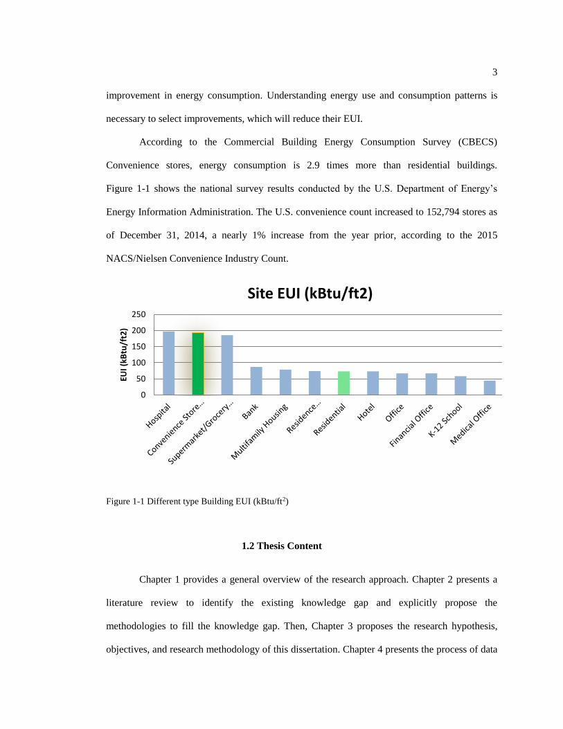
According to the Commercial Building Energy Consumption Survey (CBECS)
Convenience stores, energy consumption is 2.9 times more than residential buildings.
Figure 1-1 shows the national survey results conducted by the U.S. Department of Energy’s
Energy Information Administration. The U.S. convenience count increased to 152,794 stores as
of December 31, 2014, a nearly 1% increase from the year prior, according to the 2015
NACS/Nielsen Convenience Industry Count.
Figure 1-1 Different type Building EUI (kBtu/ft2)
1.2 Thesis Content
Chapter 1 provides a general overview of the research approach. Chapter 2 presents a
literature review to identify the existing knowledge gap and explicitly propose the
methodologies to fill the knowledge gap. Then, Chapter 3 proposes the research hypothesis,
objectives, and research methodology of this dissertation. Chapter 4 presents the process of data
0
50
100
150
200
250
EUI
(kB
tu/f
t2)
Site EUI (kBtu/ft2)

4
collection, baseline identification and chapter 5 covers demonstration CUSUM technique for the
monitoring and targeting (M&T) in convenience stores. Finally, Chapter 7 concludes the
dissertation conclusion and recommendations for future studies.
5
Chapter 2
Literature Review
This chapter presents a critical literature review on the building monitoring and
targeting and looks further into the method, description and history, along with the tools
required for this study. Section 2.1 provides a summary of the Monitoring & Targeting in the
building. Section 2.2 presents an overview of the Inverse Energy Modeling. Section 2.3 reviews
Convenience Characteristics.
2.1 Monitoring & Targeting
Energy monitoring and targeting is primarily a management technique that uses energy
information as a basis to eliminate waste, reduce and control current level of energy use and
improve the existing operating procedures. It builds on the principle “you can’t manage what
you don’t measure.”. Energy efficiency is one of the easiest and most cost effective ways to
combat climate change, clean the air we breathe, improve the competitiveness of our businesses
and reduce energy costs for consumers. The Department of Energy is working with universities,
businesses and the National Labs to develop new, energy-efficient technologies while boosting
the efficiency of current technologies on the market (Energy Monitoring and Targeting).
Monitoring and Targeting (M&T) is one of the main strategies deployed to effectively
supervise energy consumption in industrial and commercial buildings and it does so linking
measured energy use and statistical tools. Its purpose is to relate site energy consumption’s data
to weather, production or other operational measures. This allows building operators to get a
better understanding of how energy use in their facility is linked to internal processes, occupant
schedules and activities, ambient conditions or a combination of these factors. M&T essential

6
elements are data recording, monitoring, setting energy targets, analyzing, comparing, reporting
and controlling energy consumption (Guillermo and Freihaut, 2014). No standardized,
systematic, protocol-based techniques are currently in widespread use (Stuart, G. and team
2007). M&T can be a valuable tool to detect avoidable energy waste that might otherwise
remain hidden. The U.S. Department of Energy (DOE) advances building energy performance
through the development and promotion of efficient, affordable, and high impact technologies,
systems, and practices. The long-term goal of the Building Technologies Office is to reduce
energy use by 50%, compared to a 2010 baseline. To secure these savings, research,
development, demonstration, and deployment of next-generation building technologies are
needed to advance building systems and components that are cost-competitive in the market.
DOE develops, demonstrates, and deploys a suite of cost-effective technologies, tools,
solutions, best practices, and case studies to support energy efficiency improvements in
commercial buildings. DOE also spearheads the Better Buildings Challenge, a public-private
partnership committed to a 20% reduction in commercial building energy use by 2020
(Buildings, Office of Energy Efficiency & Renewable Energy). The essential elements of M&T
system are:
• Measuring and recording energy consumption
• Analyzing -Correlating energy consumption to a measured output, such as production
quantity and/or set of weather conditions
• Comparing energy consumption of a specific facility to an appropriate standard or
benchmarking data set of similar type facilities
• Setting targets to reduce or control energy consumption
• Comparing monitored energy consumption to the set target on a regular basis
• Reporting the results including any variances from the targets which have been set
• Implementing measures to correct any increased energy use variances Observed
7
Documenting lessons learned about reductions in energy use resulting from energy
conservation measures applied
McKinsey suggests that companies can double the efficiency of their operations , e.g.
data centers, through more disciplined management, thereby reducing energy costs and
greenhouse gas emissions. Specifically, companies need to manage their technology assets more
aggressively so existing servers can work at much higher utilization levels. They also need to
make significant improvements in forward planning of data center needs in order to get the most
from their capital spending.
2.2 Inverse Energy Modeling
The ASHRAE Handbook of Fundamentals (2009) classifies building energy use
analysis methods into two categories; forward (classical) modeling and data driven (inverse)
modeling. Forward modeling approach is suitable for energy analysis of new building designs.
This approach needs physical geometry, heat transfer characteristics of the building envelope,
characteristic and efficiency of the equipment in different systems, and many other physical
details as input. Blast, DOE-2, TRYNSYS, and EnergyPlus are examples of computer software
programs for forward modeling. Forward modeling tries to estimate the energy use of the
building by building its physical model, whereas inverse modeling tries to analyze the building
energy use by developing a databased, mathematical model of its as-operated energy use
characteristics. This mathematical model is created with available data from the building e.g.
utility bills as well as data from sensors installed in the building.
Inverse modeling (data driven) energy analysis is being used with three different
approaches; empirical or“BlackBox”, calibrated simulation, Grey Box models.
8
In the Black Box model, the relationship between building energy use (or any other
response variable the researcher is interested in) and the independent variable (usually climatic
variables e.g. outside air temperature) is described with a regression model (Kissock, J. and
team, 2002).
In calibrated simulation, the researcher tries to adjust the inputs of a forward model
with the results of the inverse model so that the forward model energy use predictions match
with the building energy use as is. In Gray Box approach, first a physical model is defined by
formulas that describe the structural and physical configuration of the building and different
systems in the building. Then, using these formulas and statistical analysis, specific key
parameters and overall physical characteristics of the building would be identified (Salimifard
and Freihaut, 2014). Inverse modeling (data driven) method is suitable for existing buildings,
especially those which are candidates for energy efficiency retrofits. This method is based on
the development of a mathematical equation (usually resulting from a regression type of
analysis), that relates the building energy use with the buildings energy drivers (weather,
occupant activity and/or production or a combination of these). Inverse modeling uses the actual
energy consumption (electricity or gas) rather than the heat interactions to model the building.
In recent years, some researchers have proposed hybrid models that employ simultaneously
forward and inverse modeling as a solution to the limitations of the uncertainty of the variables
involved in this type of analysis (Xu and Freihaut, 2012).
Inverse modeling can be applied for identifying more accurate ECMs and planning
more successful energy retrofits as well as enabling operational analysis, real time control, and
fault detection. Clearly, the more detailed metering and monitoring in a building, meaning the
more available data from the building, would enable engineers to achieve more accountable and
accurate results from any type of data driven modeling approach being followed (Reddy and
Claridge, 2000). In general, a one independent variable regression is the simplest and more

9
common approach to generate the building energy model. However, according to Katipamula,
et al. (1998), a multivariate regression may provide better accuracy, as well as physical insight.
They indicated that in commercial buildings, electrical and heating use is a function of climatic
conditions, building characteristics, building usage, system characteristics and type of heating,
ventilation, and air conditioning. The inconvenience of this approach is that measuring these
elements and finding the correct relationships between them is generally too complex, time
consuming and labor cost intensive. Subsequently, this would require data from multiples
sources that are not always available in a real installation and would limit the use of M&T
(Vaino, 2008).
Typically, the outside air temperature is considered the main energy consumption driver
(Beggs, 2002). If the outside air temperature is selected as the independent variable (or it is used
in conjunction with other parameters), it is necessary to choose how it should be utilized in
fitting the data according to the measured response parameter (electricity or gas). Although
various methods have been proposed, two have been identified as the most promising: the
variable degree-day method (VDD) and the mean monthly temperature method (MMT). The
VDD was introduced by Lt- Gen. Sir Richard Strachey around 1800 for crop growing analysis
as a means of identifying the length of the growing season. Later, in the 20th century, his
concept was employed in building energy analysis (CIBSE, 2006). Degree-days are essentially
the summation of the duration of temperature differences from a given reference temperature
over time, and hence they capture both extremity and duration of outdoor conditions. As noted,
the differences are calculated between a reference temperature and the outdoor air temperature.
In the case of heating, the degree days are defined as variable heating degree days
(HDD) and they quantify the values below the reference temperature. On the opposite side, for
cooling, the degree days are defined as variable cooling degree days (CDD) and they quantify
the temperatures above the reference temperature. In buildings, the reference temperature is

10
known as the balance point temperature. This value represents the outdoor air temperature when
neither the heating or cooling system is needed to run to maintain comfort conditions. From a
heat exchange point of view, the balance temperature represents the outdoor temperature at
which the building system is able to balance its internal thermal production rate with the rate of
exchange of environmental heat conditions (CIBSE, 2006). The balance temperature is critical
to obtain the correct calculation of the heating or cooling degree-day values. However, its
determination is not a straightforward procedure.
Nevertheless, to have an accurate model, it can be useful to identify a specific value,
and the method used to determine it, even if there are many assumptions needed to be made
(CIBSE, 2006). It is to be noted that some investigators recommend that VDD should never be
adopted for very short time scales analysis (hourly and daily) if a reasonable degree of accuracy
is required (Day and Karayiannis, 1999). This is because of the potentially wide range of
temperature deviations from the base temperature that could be present for short periods of
time. According to their conclusions, for the degree-days, the uncertainty decreases as the time
frame increases.
Historically, degree days have been publish in a standard base temperature of 60 °F,
because it is supposed that, in general, most buildings will start cooling and heating at that
temperature. However, it cannot be assumed that convenience stores, or any internally load
dominated building systems, have the standard base temperature as the balance temperature. In
this work, buildings have cooling during almost the entire year, so there is not any balance
temperature and the temperature at which cooling is observed to be required to maintain
comfort was supposed as a base temperature for building and CDD was taken.
The other frequently used technique to match the air temperature with the measured
energy parameter (electricity or gas) consists in using the average monthly dry bulb
temperature. This method is known as monthly mean temperature method (Reddy et al, 1997).
11
This procedure is generally preferred because it is simpler than the degree days method
(Levermore, 2000) and had been applied in grocery stores and other types buildings with results
in the acceptable range of tolerance (Eger and Kissock, 2010; Effinger et al., 2011; Xu and
Freihaut, 2012). For this method, monthly mean daily values for the energy use and temperature
are recommended as having better model accuracy (Reddy et al, 1997). The MMT consists in
plotting the monthly mean energy use (electricity or gas) versus mean monthly outdoor air
temperature and calculating a regression that could have two or more change points. There are
four MMT general models corresponding to the number of fitting parameters utilized: 2, 3, 4
and 5 parameters. Each of the models is applicable to a different type of temperature-energy use
relation, as shown in Figure 1- 4 (Reddy et al, 1997). In the case of cooling, the slope of the best
fit will be positive, whereas the slope will be negative if it is heating. The change point, in
physical terms, represents the building balance temperature. In the 2P, 3P and 4P models, there
is just one change point. The 5P model only applies to buildings that are heated and cooled with
only one energy source. The equations that define each model are indicated in Table 2-1.
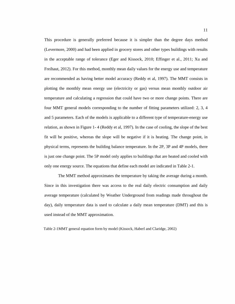
The MMT method approximates the temperature by taking the average during a month.
Since in this investigation there was access to the real daily electric consumption and daily
average temperature (calculated by Weather Underground from readings made throughout the
day), daily temperature data is used to calculate a daily mean temperature (DMT) and this is
used instead of the MMT approximation.
Table 2-1MMT general equation form by model (Kissock, Haberl and Claridge, 2002)

12
There are several methods to define change point and general equation forms. The
ASHRAE Inverse Modeling Toolkit (IMT) is one of the most popular methods. IMT is a
FORTRAN 90 application for calculating linear, change-point linear, variable- based degree-
day, multi-linear, and combined regression models. The development of IMT was sponsored by
ASHRAE research project RP-1050 under the guidance of Technical Committee 4.7; Energy
Calculations (K.Kissock). IMT software is a MS-DOS based application and data input is
manual, using a .TXT file. This process is time consuming and it is not practical to analyze
multiple buildings. Further work is necessary to develop a more user friendly application that
allows one to develop models faster and provides various models results at the same time
(Guillermo Orellana and Freihaut, 2014). Microsoft Excel can be very helpful to run regression
analysis with large amounts of data. Compared to the ASHRAE IMT method, the Microsoft
Excel application is much more convenient. This investigation will show later there is no
appreciable difference in results between these two methods. Both methods require energy data
and outdoor air temperatures as inputs and the outputs consist in the regression equation and the
statistical elements necessary to validate the equation.
Guillermo Orellana presents and develops a methodology to monitor and target energy
use in convenience stores. The main objective of his research was to develop a methodology to
13
audit, monitor and target energy use in convenience stores to detect deviations from whole
building energy use base line.
This study develops methodology by using inverse energy modeling and the application
of the cumulative sum graph as the main tracking tool for continually monitoring main end-
users of convenience stores, Refrigeration, HVAC and Lighting, which would give more
accuracy to interpret building energy consumption deviation. In this work, inverse modeling
uses daily data of building energy use as well as energy used by the main sub-systems. These
data are used to generate the baseline energy use fingerprints of each convenience store. This
study shows importance of sub-systems energy tracking to identify whole building energy
consumption deviation.
2.3 Convenience Store Characteristics
According to NACS Constitution and Bylaws, the NACS Definition of a Convenience
is:
A retail business with primary emphasis placed on providing the public a convenient
location to quickly purchase from a wide array of consumable products (predominantly food or
food and gasoline) and services (Travis Madsen and team, 2005)
While such operating features are not a required condition of membership, convenience
stores have the following characteristics:
While building size may vary significantly, typically the size will be less than
5,000 square feet;
Off-street parking and/or convenient pedestrian access;
Extended hours of operation with many open 24 hours, seven days a week;
14
Product mix includes grocery type items, and includes items from the following
groups: beverages, snacks (including confectionery) and tobacco.
Consumers are embracing convenience stores like never before. An average selling fuel
has around 1,100 customers per day, or more than 400,000 per year. Cumulatively, the U.S.
convenience industry alone serves nearly 160 million customers per day and 58 billion
customers every year. The U.S. convenience count increased to a record 152,794 stores as of
December 31, 2014, a 1% increase from the year prior, according to the 2015 NACS/Nielsen
Convenience Industry Count. One challenge in convenience stores management is that these
building locations are spread out over thousands of miles and, in general, depend on a
centralized office to oversee all their operational requirements. This includes energy
management, which can be complex and difficult since equipment operation supervision and
maintenance is done remotely for an appreciable number of stores. Therefore, the energy
management department should be able to analyze information coming from multiple building
and be able to take the appropriate decisions to keep the stores operating efficiently.
The chain that facilitated the data and information for this research is located in the U.S.
Mid-Atlantic region and chain operates two types of stores: fuel stores and non-fuel stores. The
first ones are the combination of a gas station, while the second group is simple the convenience
with no gas pump service. However, both types of establishments share the same general
internal configuration and costumer services, with the exception of the gasoline refueling. In
general, the internal division comprises three main parts. The center area is occupied by the dry
products section; on one side is the deli area, where all the hot beverages and foods are prepared
and on the opposite side is the refrigerated aisle where the freezers and refrigerators are located.
The back of the is where the dry merchandize deposits are situated and it is accessed thru the
deli area. Additionally, there is a door near the refrigerated area that connects with the outside
and where all products for inventory replacement are fed into the building. In total, there are

15
three doors (including the main door at the front and the trash door) that connect with the
outside. The mechanical systems are directly above the ceiling and this is all covered by a gable
roof. A graphical depiction of the can be seen in figure 2-1 with a location of the equipment for
a typical (Orellana and Freihaut, 2014).
Figure 2-1 Generic floor plan
The predominant weather at the locations of the selected stores is classified as mixed
cold and hot and humid. In general, the surroundings are characterized as suburban locations
with small to medium size commercial buildings and residential houses near the store. In the
immediate environs of the building, there is a parking lot that is at times shared with other
nearby businesses and vegetation is as tall as the store. In general, all exterior walls are exposed
to the outer the elements. Nearly all the stores operate 365 days a year and 24 hours a day.
Two main observation results were the most relevant from a site visit:
1. The side-door, where the products feed into the store, is often left open. This is a
consequence of the inventory restocking process that occurs along the day and, many times, the
16
workers leave this door open. This entrance directly connects thru a hallway to the main sales
area. This means that cold or warm air (depending on the season) is entering the constantly,
generating an unnecessary heat or cooling load inside the building. The combined effect of this
door, plus the infiltration and exchange air effects of the main customer entry, causes important
thermal interactions with the outside environment that can lead to a higher heating, ventilation
and air conditioning energy use in certain times of the year.
2. There are no physical barriers that separate the hot, humid air coming from the deli
zone and the cold, dry air coming from the refrigerated casings. The zone of interaction is the
middle area, where the dry products are located. Occasionally, an open case refrigerator could
be in this area. In general, this condition could be found in supermarkets. However, the footprint
of supermarkets is considerably larger than convenience stores, meaning that the zone of
interaction is larger and the effect of the temperature gradient is dissipated. The issue in the
convenience is that the selling area is much smaller and air mixing is more likely to occur, with
refrigerators receiving warm air from the hot food area, leading to higher energy consumption.
All these factors are relevant to explain, in part, the probable higher energy
consumption per building area relative to similar buildings like supermarkets. In addition, these
findings were necessary to further understand the building energy model. In general, the
interaction of the inside air with the outside is constant not only thru the service doors but
because of the high client rotation. Normally, the customers spend less than five minutes inside
the building, indicating that people are coming in and going out constantly. This observation
gives strong signs that outdoor air temperature and costumer count could be important energy
use drivers. As a reference, the typical equipment found in the stores is indicated in table 2-2
(Orellana and Freihaut, 2014).

17
Table 2-2 Equipment
Hot Equipment
Cold Equipment
Other Equipment
Coffee machine Cold pan service station Cashing machine
Condiment stand Cold Products dispenser ATM
Toaster Beverage cabinet HVAC Systems
Food warmer Milkshake/Frozen milkshake dispenser Gas Heater
Heated cabinets Ice Tea/Coffee dispenser
Rethermalizer Open Refrigerator
Closed refrigerators
Ice maker
Closed freezers
Refrigerated casings

18
Chapter 3
Dissertation Hypothesis, Objectives, and Methodology
The goal of this study is to presents a method for establishing inverse modeling analysis
tools to enable implementation of a continuous efficiency improvement loop (CEIL)at energy
intensive convenience stores.
Sections 3.1 and 3.2 present the research hypothesis and objectives, respectively.
Section 3.3 presents the proposed methodology to identify building energy baseline and
determine the end-use cause of energy use deviations. And section 3.4 provides an overview of
the tasks for this dissertation.
3.1 Research Hypothesis
Table 3-1 presents the research hypothesis. The problem statement and the literature
review in Chapter 2 are used to define the research hypothesis. This dissertation presents a tool
to enable Continues Efficiency Improvement Loop (CEIL) implementation based on identifying
end-use energy consumption pattern , establishing an expected energy use baseline and ongoing
data monitoring to determine deviations from the expected energy use. This method will help to
inform owners and operators as to what operational changes can be made to reduce energy
consumption. Continually monitoring the energy consumption of convenience stores in order to
identify typical energy use patterns is necessary. And the results of this hypothesis can support
retrofit projects to assess different Energy Efficient Measures (EEMs) in a short period of time.
This establishment allows existing city benchmarking and disclosure ordinance
programs for major U.S. cities to collect lessons in order to provide a better evaluation of

19
performance of building energy consumptions, particularly high customer turnover retail
facilities.
Table 3-1 Proposed research hypothesis of this dissertation
Research Hypothesis:
Continues Efficiency Improvement Loop (CEIL) Can be
Accomplished Based by Energy Signature and Energy Monitoring at
Energy Intensive Convenience Stores
3.2 Dissertation Objectives
This dissertation defines three objects presented in Table 3-2 to conduct the study. In
the first step, a regression framework is defined to an energy consumption baseline. Then, based
on the identified baselines, there is a need to monitor and analyze building energy consumption
ongoing data.
The last objective is demonstrating first and second objectives approaches for case
study.
Table 3-2 Proposed research objectives of this dissertation
Research Objectives:
1- Identify store specific energy use baselines with data
monitoring followed by regression analysis.
2- Analyze ongoing data based on baseline with Cumulative
Sum (CUSUM) method.
3- Determine energy deviation accumulations from store
specific whole building and end-use baselines.

20
3.3 Research Methodology
An energy signature, fingerprint, is a graph of consumption energy against some
independent parameter that at least partially determines the amount of energy use and
establishes a pattern of energy consumption.
There are two commonly used forms of energy signatures for buildings:
1) Graph of energy vs. Degree-Days using monthly or weekly degree-days;
2) Graph of energy vs. Average daily or monthly temperature.
In this investigation, we are working on electric energy consumption fingerprints of
refrigeration, HVAC and lighting end uses vs. average daily and average monthly temperature.
Regression is a statistical technique that estimates the dependence of a variable of interest, such
as energy consumption, on one or more independent variables, such as ambient temperature. It
can be used to estimate the effects on the dependent variable of a given independent variable
while controlling for the influence of other variables at the same time. It is a powerful and
flexible technique that can be used in a variety of ways when measuring and verifying the
impact of energy efficiency projects (Bonneville Power Administration, 2012).
The regression model attempts to predict the value of the dependent variable based on
the values of independent, or explanatory, variables such as weather data.
The dependent variable is typically energy use and Independent Variable, a variable
whose variation explains variation in the outcome variable; for M&V, weather characteristics
are often among the independent variables.
This dissertation considers the results of the regression model as the building energy
signature and provides whole building and refrigeration, HVAC and lighting baselines based

21
on electricity consumption as the dependent variable and outdoor temperature as independent
variable.
In order to determine the end-use cause of energy use deviations the CUSUM M&T
analysis tool is applied. The CUSUM M&T analysis tool allows facility managers to
immediately determine the end-use cause of energy use deviations observed in the energy use
CUSUM reporting.
CUSUM is a powerful technique for developing management information regarding the
energy-consuming system. It distinguishes between faults or improvements events affecting on
system. CUSUM stands for 'cumulative sum of differences', where 'difference' refers to
differences between the actual consumption and the predicted or expected energy consumption
from an energy baseline represented by a regression analysis of data. If consumption is
following the established baseline, the differences between the actual consumption and
predicted consumption will be small and randomly either positive or negative. In over the
baseline temperature range, the cumulative sum of these differences will stay near zero. Once a
change in pattern occurs due to the presence of a fault or to some improvement in the
consumption monitored, the distribution of the differences about zero becomes less symmetrical
and the cumulative sum, CUSUM, increases or decreases with time.
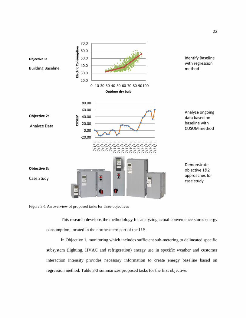
3.4 Overview of the Tasks within the Objectives
Each of the dissertation objectives has several tasks critical to the accomplishment of
specified objectives. Figure 3-1 summarizes the proposed tasks for three objectives of this
dissertation.
22
Objective 1:
Building Baseline
Identify Baseline with regression method
Objective 2:
Analyze Data
Analyze ongoing data based on baseline with CUSUM method
Objective 3:
Case Study
Demonstrate objective 1&2 approaches for case study
Figure 3-1 An overview of proposed tasks for three objectives
This research develops the methodology for analyzing actual convenience stores energy
consumption, located in the northeastern part of the U.S.
In Objective 1, monitoring which includes sufficient sub-metering to delineated specific
subsystem (lighting, HVAC and refrigeration) energy use in specific weather and customer
interaction intensity provides necessary information to create energy baseline based on
regression method. Table 3-3 summarizes proposed tasks for the first objective:
20.0
30.0
40.0
50.0
60.0
70.0
0 10 20 30 40 50 60 70 80 90100
Ele
ctri
c C
on
sum
pti
on
Outdoor dry bulb
-20.00
0.00
20.00
40.00
60.00
80.00
7/1
/11
7/3
/11
7/5
/11
7/7
/11
7/9
/11
7/1
1/1
1 7
/13
/11
7/1
5/1
1 7
/17
/11
7/1
9/1
1 7
/21
/11
7/2
3/1
1 7
/25
/11
7/2
7/1
1 7
/29
/11
7/3
1/1
1
CU
SUM

23
Table 3-3 Proposed tasks for the first objective
Tasks for the First
Objective:
1
Identify all independent variables to be included in the regression
model
2 Collect data and Synchronize data
3 Graph the data
4 Select and develop the regression model
5 Determine the Quality of the Regression Model
While Objective 1 focuses on the energy baseline identification of sub-metered energy
consumption, Objective 2 focuses on applying the building energy utilization data and
associated CUSUM M&T analysis tool which allows facility managers to immediately
determine the end-use cause of energy use deviations observed in the energy use CUSUM
reporting. Table 3-4 lists the proposed tasks to conclude the second objective.
Table 3-4 Proposed tasks for the second objective
Tasks for the Second
Objective:
1 Derive the equation of the baseline
2 Calculate the expected energy consumption based on the
equation
3 Calculate the difference between actual and calculated energy
use
4 Compute CUSUM
5 Plot the control chart and the CUSUM graph over the time
Objective 3 includes a demonstration case study with the use of proposed approaches
established in Objective 1&2 to investigate building energy performance. Table 3-5 illustrates
the proposed tasks for the third objective.

24
Table 3-5 Proposed tasks for the third objective
Tasks for
the Third
Objective:
1 Identify case study
2 Perform detailed Baseline identification steps, CUSUM and Control
Chart
It is important to note that in this study the electricity consumption data from the main
meter and refrigeration, HVAC and lighting sub-meters in 20 convenience stores in the
northeast U.S. during 2011-2012 was utilized.
25
Chapter 4
Identification of Baseline for Convenience Stores
This chapter presents the results of building End-users Energy baseline identification
for convenience stores. Section 4-1 presents the Convenience Stores dominant energy
consumption users. Section 4-2 provides a summary for the process of data collection, there is a
comparison between Main-meter and Sub-meters energy consumption trending in section 4-3.
Section 4-4 presents Weather Data Characterization, Section 4-5 illustrates regression
techniques for identify baseline and section 4-6 discusses on observations.
4.1 Convenience Store
According to the Commercial Building Energy Consumption Survey (CBECS)
Convenience stores, energy consumption is 2.9 times more than residential buildings. This
dissertation studies 20 convenience stores in the northeast U.S. Except domestic hot water,
which runs by natural gas, electricity provides required energy for other end-users.
In this study, the electricity consumption data from, Refrigeration, HVAC and Lighting,
in 20 convenience stores were investigated. Figure 4-1 shows EUI for 20 stores in 2012.

26
Figure 4-1 Stores EUI for 2012
According to figure 4-2 the most dominant electric consumption is related to
refrigeration, HVAC and lighting and which is this investigation focused on.
Table 4-1 presents some of equipment associated with RPB, RPC, etc. panels which are
not dominant electric consumption. For more details about equipment associated with RPA,
RPB, etc. panels look at appendix I.
0
100
200
300
400
500
600
Total 2012 Electricity USAGE(kBtu/ft2) Total 2012 Natural Gas USAGE(kBtu/ft2)

27
Figure 4-2 Electric consumption portion between sub-meters
Table 4-1 Some of equipment associated with panels
PNL Description
RPB Smoothie blender, Hot table, Toaster oven, etc.
RPC ATM, General purpose receipt, Slicer, Auto flush valve, etc.
RPD Fuel Dispenser, Cash register, Overall alarm, etc.
RPE
Printer manager, Time lock, Price changing motor, Security Monitor, Phone
card, etc.
RPG Canopy lighting, Air pump, etc.
RPA_Daily_Usage, 15.47%
RPB_Daily_Usage, 14.49%
RPC_Daily_Usage, 9.22%
RPD_Daily_Usage, 0.00%
RPE_Daily_Usage, 3.42%RPG_Daily_Usage,
4.11%
Refrig_Daily_Usage, 15.81%
HVAC_Daily_Usage, 16.16%
LPA_Daily_Usage, 19.66%

28
4.2 Process of Data Collection
The collected data period should be sufficient to represent the full range of operating
conditions. For example, when using monthly data for a weather-sensitive measure, the baseline
period typically includes 12 or 24 months of billing data, or several weeks of meter data. Using
a partial year may overemphasize specific seasons or average temperature levels of the year and
add uncertainty in the model or lack of application to the full temperature ranges experience in a
year.
It is vital that the collected baseline data accurately represent the operation of the
system or the particular sub-system in question HVAC, refrigeration, lighting, etc. Anomalies
in these data can have a large effect on the outcome of the study. Examining data outliers, data
points that do not conform to the typical distribution, and seek an explanation for their
occurrence is essential. Typical events that result in outliers include equipment failure, any
situations resulting in abnormal closures of the facility, and a malfunctioning of the metering
equipment. Truly anomalous data should be removed from the data set, as they do not describe
the operations prior to the installation of the measure. In term of outlier detection, the
Thompson outlier test method was conducted in this study; appendix II presents detail for this
method.
To accurately represent each independent variable, the intervals of observation must be
consistent across all variables. For example, a regression model using monthly utility bills as the
outcome variable requires that all other variables originally collected as hourly, daily, or weekly
data is converted into monthly data points over exactly the same time interval. In such a case, it
is common practice to average points of daily data over the course of a month, yielding
synchronized monthly data.
29
For visualize and explore the relationships between the dependent and independent
variables create one or more scatter plots. Most commonly, one graphs the independent
variables on the X-axis and the dependent variable on the Y axis.
4.3 Comparison of whole building and sub-meters Energy Consumption Trending
Figure 4-3 displays a scatter plot of average daily temperature and electric consumption
vs. calendar day over a three-year period of time for one store. According to this chart, the Main
Panel (whole building electric energy use), refrigeration and HVAC electric consumption
trends are in phase with the daily temperature pattern while the lighting electric consumption is
relatively constant but seasonally out of phase with main, refrigeration and HVAC electric
energy utilization time series patterns. For this particular building, convenience store, there is a
gap in the period 10/07/2012-1/26/2013 in which there was no sub-metered data collected. In
figure 4-4, figure 4-5 the data indicates a significant increase in HVAC and refrigeration energy
use with average ambient temperature during the cooling season, but relatively constant HVAC
energy use during the heating season. Figure 4-6 shows, as expected, the electricity
consumption of the building does not correlate to the outdoor weather conditions. Analyzing
end-users ongoing energy consumption data defines the reason on whole building energy
consumption deviation which will help to inform owners and operators as to what operational
changes can be made to reduce energy consumption.

30
Figure 4-3 Time Series Electric Consumption and Outdoor Temperature in 01/01/2011-10/05/2013
Figure 4-4 Refrigeration Electric Consumption and Outdoor Temperature vs. day in 01/01/2011-10/05/2013
0
0.5
1
1.5
2
2.5
0
10
20
30
40
50
60
70
80
90
100
40500 40700 40900 41100 41300 41500
Ou
tdo
or
Tem
pe
ratu
re (
F)
01/01/2011 - 10/05/2013
Electric Consumption in 01/01/2011-10/05/2013
Average Temp. (°F)
MainElectric(kBtu/ft2-day)
Refrigeration(kBtu/ft2-day)
HVAC (kBtu/ft2-day)
LPA (kBtu/ft2-day)
Ele
ctri
c C
on
sum
pti
on
(kB
tu/f
t2)
0
0.1
0.2
0.3
0.4
0.5
0.6
0.7
0
10
20
30
40
50
60
70
80
90
100
40500 40700 40900 41100 41300 41500
Ou
tdo
or
Tem
pe
ratu
re (
F)
01/01/2011 - 10/05/2013
Electric Consumption in 01/01/2011-10/05/2013
Average Temp. (°F)
Refrigeration (kBtu/ft2-day)
Ele
ctri
c C
on
sum
pti
on
(kB
tu/f
t2)

31
Figure 4-5 HVAC Electric Consumption and Outdoor Temperature vs. day in 01/01/2011-10/05/2013
Figure 4-6 Lighting Electric Consumption and Outdoor Temperature vs. day in 01/01/2011-10/05/2013
0
0.1
0.2
0.3
0.4
0.5
0.6
0.7
0
10
20
30
40
50
60
70
80
90
100
40500 40700 40900 41100 41300 41500
Ou
tdo
or
Tem
pe
ratu
re (
F)
01/01/2011 - 10/05/2013
Electric Consumption in 01/01/2011-10/05/2013
Average Temp. (°F)
HVAC (kBtu/ft2-day)
Ele
ctri
c C
on
sum
pti
on
(kB
tu/f
t2)
0
0.1
0.2
0.3
0.4
0.5
0.6
0.7
0
10
20
30
40
50
60
70
80
90
100
40500 40700 40900 41100 41300 41500
Ou
tdo
or
Tem
pe
ratu
re (
F)
01/01/2011 - 10/05/2013
Electric Consumption in 01/01/2011-10/05/2013
Average Temp. (°F)
LPA (kBtu/ft2-day)
Ele
ctri
c C
on
sum
pti
on
(kB
tu/f
t2)

32
4.4 Weather Data Characterization
The study used weather data from the closest reliable weather stations that provide
easily accessible weather station data to the public and have standardized reporting and
instrument maintenance protocols. Based on the American Society of Heating, Refrigeration,
and Air-conditioning Engineers (ASHRAE) classification, all studied convenience stores are
located in “cool-humid” climate region.
4.5 Regression for Baseline Identification
To create energy baseline based on regression method for Whole Building,
Refrigeration, HVAC and Lighting at each twenty studied convenience stores, Outdoor air
temperature considered as independent variable and electricity consumption for each main
meter and sub-meters applied as a dependent variable. In this study Outdoor Temperature is
daily average temperature (calculated by Weather Underground from readings made throughout
the day) and electricity consumption is actual daily electric consumption. Availability and
accuracy of energy consumption commodities are vital for a proposed energy baseline based on
the building energy use.
There are various types of linear regression models that are commonly used for M&V.
In certain circumstances, other model functional forms, such as second-order or higher
polynomial functions, can be valuable. The M&V practitioner should always graph the data in a
scatter chart to verify the type of curve that best fits the data. The ASHRAE Inverse Model
Toolkit, a product that came out of research project RP-1050, provides FORTRAN code for
automating the creation of the various model types described below. However, by creating
spreadsheet in Excel and proper equation you can create your model faster than Inverse Model

33
Toolkit. Figure 4-7 shows comparison between results of ASHRAE Inverse Modeling Toolkit
(IMT) and Excel Regression Model spreadsheet (ERM).
R-Square for IMT=0.824 ERM=0.825
Figure 4-7 Comparison of Inverse Model Toolkit and author’s own spreadsheet output
R-Square for IMT=0.927 ERM=0.928
Figure 4-8 Lighting Electric Consumption and Outdoor Temperature vs. Day
4.00
9.00
14.00
19.00
24.00
29.00
34.00
39.00
0.0 20.0 40.0 60.0 80.0 100.0
Ave
rage
Mai
nEl
ect
ric(
kBtu
/ft2
-mo
nth
)
Average Temperature (F)
IMT
ERM
Real Data
3.00
3.30
3.60
3.90
4.20
4.50
4.80
5.10
5.40
5.70
6.00
0.0 20.0 40.0 60.0 80.0 100.0
Ave
rage
Re
frig
era
tin
El
ect
ric(
kBtu
/ft2
-mo
nth
)
Average Temperature (F)
IMT
ERM
Real Data

34
R-Square for IMT=0.889 ERM=0.882
Figure 4-9 Lighting Electric Consumption and Outdoor Temperature vs. day
R-Square for IMT=0.165 ERM=0.159
Figure 4-10 Lighting Electric Consumption and Outdoor Temperature vs. day
0.00
0.50
1.00
1.50
2.00
2.50
3.00
3.50
4.00
0.0 20.0 40.0 60.0 80.0 100.0
Ave
rage
HV
AC
(kB
tu/f
t2-m
on
th)
Average Temperature (F)
IMT
ERM
Real Data
3.00
3.50
4.00
4.50
5.00
5.50
6.00
6.50
7.00
0.0 20.0 40.0 60.0 80.0 100.0
Ave
rage
LP
A E
lect
ric(
kBtu
/ft2
-mo
nth
)
Average Temperature (F)
IMT
ERM
Real Data

35
Figure 4-11 illustrates the major models used for temperature-dependent loads. The top
row illustrates 2-parameter heating and cooling models; the second row illustrates 3-parameter
models; the third row illustrates 4-parameter models; and the bottom row illustrates a 5-
parameter combined heating and cooling model.
Figure 4-11 Change-point Linear and Multiple-Linear Inverse Building Energy Analysis Models
(ASHRAE Research Project 1050-RP, Development of a Toolkit for Calculating Linear)
36
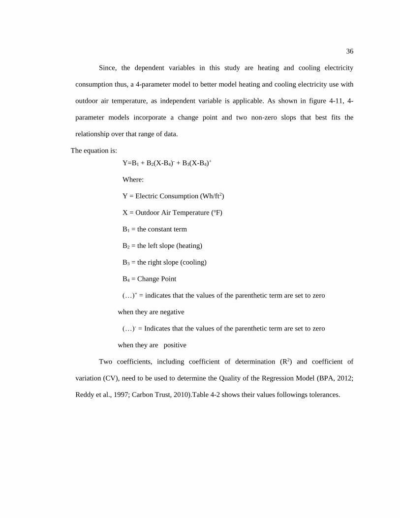
Since, the dependent variables in this study are heating and cooling electricity
consumption thus, a 4-parameter model to better model heating and cooling electricity use with
outdoor air temperature, as independent variable is applicable. As shown in figure 4-11, 4-
parameter models incorporate a change point and two non-zero slops that best fits the
relationship over that range of data.
The equation is:
Y=B1 + B2(X-B4)- + B3(X-B4)+
Where:
Y = Electric Consumption (Wh/ft2)
X = Outdoor Air Temperature (oF)
B1 = the constant term
B2 = the left slope (heating)
B3 = the right slope (cooling)
B4 = Change Point
(…)+ = indicates that the values of the parenthetic term are set to zero
when they are negative
(…)- = Indicates that the values of the parenthetic term are set to zero
when they are positive
Two coefficients, including coefficient of determination (R2) and coefficient of
variation (CV), need to be used to determine the Quality of the Regression Model (BPA, 2012;
Reddy et al., 1997; Carbon Trust, 2010).Table 4-2 shows their values followings tolerances.

37
Table 4-2 Recommended tolerances
R2 CVRMSE
ASHRAE Guideline 14-2002 > 0.80 < 20% for periods < 12 months,
CVRMSE < 25% for period of 12 to 60
months
The coefficient of multiple determinations (R2) represents how well data points fit a line
or curve and it is defined as the percentage of the response variation that is explained by a linear
model. In general, the higher the R2 (closest to 1), the better the model fits the data (MiniTab,
2013). Equation 4-1 is used to find the R2 of a regression.
𝑅2 = 1 −∑ (𝐴−𝑀)^2𝑛
∑ (𝐵−𝑀)^2𝑛 Equation (4-1)
Where,
A is the observed values
M is the mean of the values
B is the fitted values
n is the number of the observation
The CVRMSE is the root mean squared error (RMSE) normalized by the average y
value. Normalizing the RMSE makes this parameter a non-dimensional value that describes
how well the model fits the data. It is not affected by the degree of dependence between the
independent and dependent variables, making it more informative than R2 for situations where
the dependence is relatively low (BPA, 2012). Equation 1-4, defines the CVRMSE.
𝐶𝑉𝑅𝑀𝑆𝐸 = 100√[
∑(𝐴−𝐵)2
(𝑛−𝑝)]
𝑀 Equation (4-2)
Where,
A is the observed values

38
M is the mean of the values
B is the fitted values
n is the number of the observation Where,
p is the number of the variable
In the case that a variable is zero, close to zero or negative, the CVRMSE can be
misleading because the mean value can be close to zero. In general, the coefficient of variation
of a model can be considered reasonable, if the variable contains only positive values not close
to zero (IDRE, 2013).
4.6 Discussions on the Stores Energy Consumption Baseline
Statistical correlation analyses can strengthen the robust prediction of energy
performance in convenience stores. In Guillermo and Freihaut study regression methods were
used to establish expected energy use baselines for whole building this study uses refrigeration,
HVAC and lighting energy used in the sub-metered stores data sets in addition to whole
buildings; to present importance of sub-users energy consumption analysis to interpolate whole
building energy trend. Figures 4-12 to 4-15 display the baselines for whole building
refrigeration, HVAC and lighting end use energies.

39
Equation: Consumption=790 + 0.9(Temperature-55)- + 5.63(Temperature -55)+
Multiple R: 0.87, CV: 2.6 %, Standard Error: 3.35, Observations: 921
Figure 4-12 Refrigeration Electric Energy Consumption Baseline
Equation: Consumption=29.35 + 0.13(Temperature-56)- + 0.39(Temperature -56)+
Multiple R: 0.87, CV: 7.3 %, Standard Error: 3.35, Observations: 921
Figure 4-13 Refrigeration Electric Energy Consumption Baseline
620.0
720.0
820.0
920.0
1,020.0
1,120.0
1,220.0
0 10 20 30 40 50 60 70 80 90 100
Mai
n E
lect
ric
Co
nsu
mp
tio
n (
Btu
/ft2
-day
)
Outdoor Temperature (F)
Main_Daily_Usage(Btu/ft2)
Baseline
50.0
70.0
90.0
110.0
130.0
150.0
170.0
190.0
210.0
230.0
0 10 20 30 40 50 60 70 80 90 100
Ele
ctri
c C
on
sum
pti
on
(B
tu/f
t2-d
ay
Outdoor Temperature (F)
Refrigeration_Daily_Usage(Btu/ft2)
Baseline
40
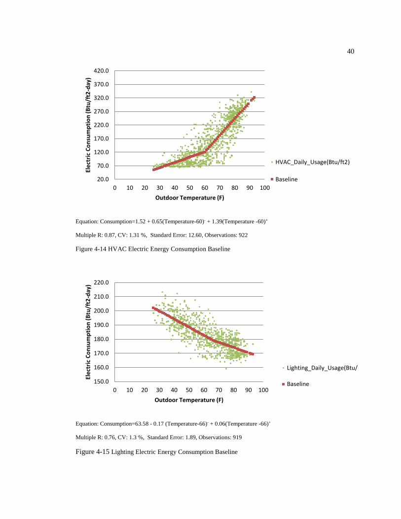
Equation: Consumption=1.52 + 0.65(Temperature-60)- + 1.39(Temperature -60)+
Multiple R: 0.87, CV: 1.31 %, Standard Error: 12.60, Observations: 922
Figure 4-14 HVAC Electric Energy Consumption Baseline
Equation: Consumption=63.58 - 0.17 (Temperature-66)- + 0.06(Temperature -66)+
Multiple R: 0.76, CV: 1.3 %, Standard Error: 1.89, Observations: 919
Figure 4-15 Lighting Electric Energy Consumption Baseline
20.0
70.0
120.0
170.0
220.0
270.0
320.0
370.0
420.0
0 10 20 30 40 50 60 70 80 90 100
Ele
ctri
c C
on
sum
pti
on
(B
tu/f
t2-d
ay)
Outdoor Temperature (F)
HVAC_Daily_Usage(Btu/ft2)
Baseline
150.0
160.0
170.0
180.0
190.0
200.0
210.0
220.0
0 10 20 30 40 50 60 70 80 90 100
Ele
ctri
c C
on
sum
pti
on
(B
tu/f
t2-d
ay)
Outdoor Temperature (F)
Lighting_Daily_Usage(Btu/ft2)
Baseline

41
By using the baseline equation, we can find out how much electric consumption is
expected to be used for each end use by simply inputting the average outside air temperature as
an “x” value and calculating the expected electric energy consumption.
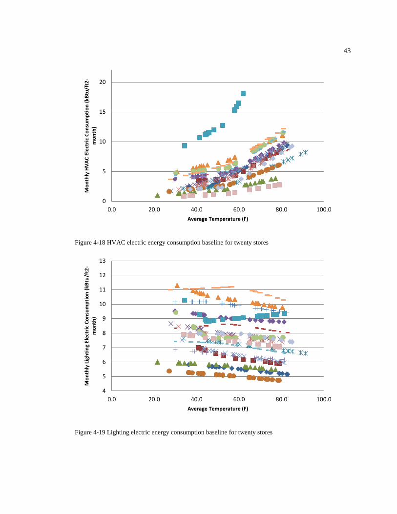
Figure 4-16 to 4-19 show twenty studied store’s identified electricity baseline for
Whole building, Refrigeration, HVAC and Lighting.
Based on the developed linear regression model, with Refrigeration and HVAC, there is
a positive correlation between electricity consumption and outdoor dry bulb temperature. And
there is not proper relationship between lighting electric consumption and outdoor dry bulb
temperature.
What is the reason of wide range of differences for different stores? It seems there is a
need for investigation of other parameters such as equipments efficiency, building orientation,
customer count, people behavior, etc., effects on energy consumption pattern in each
convenience store.

42
Figure 4-16 Whole building electric energy consumption baseline for twenty stores
Figure 4-17 Refrigeration electric energy consumption baseline for twenty stores
16
21
26
31
36
41
46
51
0.0 20.0 40.0 60.0 80.0 100.0
Mo
nth
ly M
ain
Ele
ctri
c C
on
sum
pti
on
(kB
tu/f
t2-m
on
th)
Average Temperature (F)
1.2
3.2
5.2
7.2
9.2
11.2
13.2
0.0 20.0 40.0 60.0 80.0 100.0
Mo
nth
ly R
efr
ige
rati
on
Ele
ctri
c C
on
sum
pti
on
(kB
tu/f
t2-
mo
nth
)
Average Temperature (F)
43
Figure 4-18 HVAC electric energy consumption baseline for twenty stores
Figure 4-19 Lighting electric energy consumption baseline for twenty stores
0
5
10
15
20
0.0 20.0 40.0 60.0 80.0 100.0
Mo
nth
ly H
VA
C E
lect
ric
Co
nsu
mp
tio
n (
kBtu
/ft2
-m
on
th)
Average Temperature (F)
4
5
6
7
8
9
10
11
12
13
0.0 20.0 40.0 60.0 80.0 100.0
Mo
nth
ly L
igh
tin
g El
ect
ric
Co
nsu
mp
tio
n (
kBtu
/ft2
-m
on
th)
Average Temperature (F)

44
Recent research shows that human behavior is an important factor for the energy
consumption of buildings (Lindelöf, N. Morel, 2006 & A. Mahdavi and team, 2008). On one
hand, during a cooling season, if the inside of a building is colder than the occupant thermal
comfort level requirement, occupants typically open windows. On the other hand, during a
heating season, when inside of the buildings is warmer than the thermal comfort level
requirement for the occupants, people inside of the buildings will, again, open windows. Future
studies can consider these variables to quantify the influence of these variables on the building
energy consumption pattern.
In this study the company also provided the customer count of each stores, since it was
initially thought that this could be an important energy driver. Figure 4-20 shows the
representation customer pattern for twenty stores in 2011-2012. In addition, Figure 4-21 to 4-24
show energy consumption for whole building, refrigeration, HVAC and lighting vs. customer
count of one store. Interestingly, all stores presented a clearly repetitive profile, but it seems,
there is not an outdoor air temperature related variation. Peaks were identified on January,
April, July and October, while the lower points were around February-March, May-June,
August-September and November-December. These graphs show there is no relationship
between end-users energy consumptions and customer count. The main energy consumption
driver is outdoor dry bulb temperature, but we know human beings release both sensible heat
and latent heat to the conditioned space when they stay in it. The space sensible (Q sensible) and
latent (Q latent) cooling loads for people staying in a conditioned space are calculated as:
Q sensible = N * SHG * (CLF)
Q latent = N * LHG
N = number of people in space.
SHG, LHG = Sensible and Latent heat gain from occupancy is given in 1997 ASHRAE
Fundamentals Chapter 28, CLF = Cooling Load Factor, by hour of occupancy is given in 1997
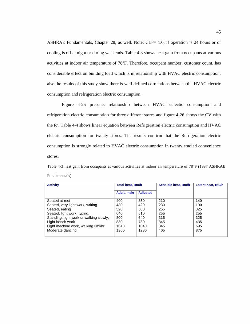
45
ASHRAE Fundamentals, Chapter 28, as well. Note: CLF= 1.0, if operation is 24 hours or of
cooling is off at night or during weekends. Table 4-3 shows heat gain from occupants at various
activities at indoor air temperature of 78°F. Therefore, occupant number, customer count, has
considerable effect on building load which is in relationship with HVAC electric consumption;
also the results of this study show there is well-defined correlations between the HVAC electric
consumption and refrigeration electric consumption.
Figure 4-25 presents relationship between HVAC eclectic consumption and
refrigeration electric consumption for three different stores and figure 4-26 shows the CV with
the R2. Table 4-4 shows linear equation between Refrigeration electric consumption and HVAC
electric consumption for twenty stores. The results confirm that the Refrigeration electric
consumption is strongly related to HVAC electric consumption in twenty studied convenience
stores.
Table 4-3 heat gain from occupants at various activities at indoor air temperature of 78°F (1997 ASHRAE
Fundamentals)
Activity Total heat, Btu/h Sensible heat, Btu/h Latent heat, Btu/h
Adult, male Adjusted
Seated at rest Seated, very light work, writing Seated, eating Seated, light work, typing, Standing, light work or walking slowly, Light bench work Light machine work, walking 3mi/hr Moderate dancing
400 480 520 640 800 880 1040 1360
350 420 580 510 640 780 1040 1280
210 230 255 255 315 345 345 405
140 190 325 255 325 435 695 875

46
Figure 4-20 Customer Count Monthly Pattern for twenty stores
0
20000
40000
60000
80000
100000
120000
140000
160000
180000
Jan
Feb
Mar
Ap
r
May Jun
Jul
Au
g
Sep
Oct
No
v
De
c
Jan
Feb
Mar
Ap
r
May Jun
Jul
Au
g
Sep
Oct
No
v
De
c
Cu
sto
me
r C
ou
nt

47
Figure 4-21 Monthly Electric Consumption of Whole building vs. Customer Count 2011-2012
22
24
26
28
30
32
44
16
6
46
19
6
46
67
7
47
14
4
47
52
5
47
75
8
50
57
7
56
62
5
57
23
2
58
01
9
61
21
5
61
66
3
61
78
2
62
01
0
62
37
0
62
84
1
64
22
8
65
27
9
65
46
2
74
78
0
77
81
4
79
21
4
80
01
7
80
77
5
Ave
rage
Mai
n
Ele
ctri
c(kB
tu/f
t2-m
on
th)
Store 1
25
27
29
31
33
35
59
07
9
60
19
2
60
51
2
61
11
2
61
57
2
62
58
8
63
46
2
63
59
6
63
60
8
63
81
7
63
82
1
64
35
3
64
58
9
64
75
3
67
76
4
73
13
6
73
49
4
76
07
6
77
66
8
77
99
9
79
76
0
80
28
6
80
79
4
82
00
1
Ave
rage
Mai
n E
lect
ric(
kBtu
/ft2
-m
on
th)
Store 2
25
27
29
31
33
35
30
49
7
33
95
7
34
81
1
35
80
1
36
16
2
36
39
2
37
10
1
43
08
0
44
27
4
45
50
5
47
06
5
50
23
9
64
22
9
70
24
4
70
96
6
72
12
2
74
06
9
74
28
3
76
83
7
84
75
5
92
05
3
92
11
3
94
48
3
11
11
43
Ave
rage
Mai
n
Ele
ctri
c(kB
tu/f
t2-m
on
th)
Store 3
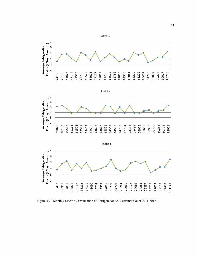
48
Figure 4-22 Monthly Electric Consumption of Refrigeration vs. Customer Count 2011-2012
2
3
4
5
6
7
44
16
6
46
19
6
46
67
7
47
14
4
47
52
5
47
75
8
50
57
7
56
62
5
57
23
2
58
01
9
61
21
5
61
66
3
61
78
2
62
01
0
62
37
0
62
84
1
64
22
8
65
27
9
65
46
2
74
78
0
77
81
4
79
21
4
80
01
7
80
77
5Ave
rage
Re
frig
era
tio
n
Ele
ctri
c(kB
tu/f
t2-m
on
th)
Store 1
2
3
4
5
6
7
59
07
9
60
19
2
60
51
2
61
11
2
61
57
2
62
58
8
63
46
2
63
59
6
63
60
8
63
81
7
63
82
1
64
35
3
64
58
9
64
75
3
67
76
4
73
13
6
73
49
4
76
07
6
77
66
8
77
99
9
79
76
0
80
28
6
80
79
4
82
00
1
Ave
rage
Re
frig
era
tio
n
Ele
ctri
c(kB
tu/f
t2-m
on
th)
Store 2
2
3
4
5
6
7
30
49
7
33
95
7
34
81
1
35
80
1
36
16
2
36
39
2
37
10
1
43
08
0
44
27
4
45
50
5
47
06
5
50
23
9
64
22
9
70
24
4
70
96
6
72
12
2
74
06
9
74
28
3
76
83
7
84
75
5
92
05
3
92
11
3
94
48
3
11
11
43
Ave
rage
Re
frig
era
tio
n
Ele
ctri
c(kB
tu/f
t2-m
on
th)
Store 3
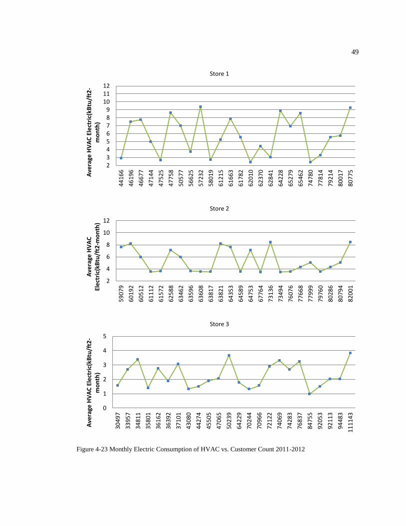
49
Figure 4-23 Monthly Electric Consumption of HVAC vs. Customer Count 2011-2012
23456789
101112
44
16
6
46
19
6
46
67
7
47
14
4
47
52
5
47
75
8
50
57
7
56
62
5
57
23
2
58
01
9
61
21
5
61
66
3
61
78
2
62
01
0
62
37
0
62
84
1
64
22
8
65
27
9
65
46
2
74
78
0
77
81
4
79
21
4
80
01
7
80
77
5
Ave
rage
HV
AC
Ele
ctri
c(kB
tu/f
t2-
mo
nth
)
Store 1
2
4
6
8
10
12
59
07
9
60
19
2
60
51
2
61
11
2
61
57
2
62
58
8
63
46
2
63
59
6
63
60
8
63
81
7
63
82
1
64
35
3
64
58
9
64
75
3
67
76
4
73
13
6
73
49
4
76
07
6
77
66
8
77
99
9
79
76
0
80
28
6
80
79
4
82
00
1
Ave
rage
HV
AC
El
ect
ric(
kBtu
/ft2
-mo
nth
)
Store 2
0
1
2
3
4
5
30
49
7
33
95
7
34
81
1
35
80
1
36
16
2
36
39
2
37
10
1
43
08
0
44
27
4
45
50
5
47
06
5
50
23
9
64
22
9
70
24
4
70
96
6
72
12
2
74
06
9
74
28
3
76
83
7
84
75
5
92
05
3
92
11
3
94
48
3
11
11
43
Ave
rage
HV
AC
Ele
ctri
c(kB
tu/f
t2-
mo
nth
)
Store 3
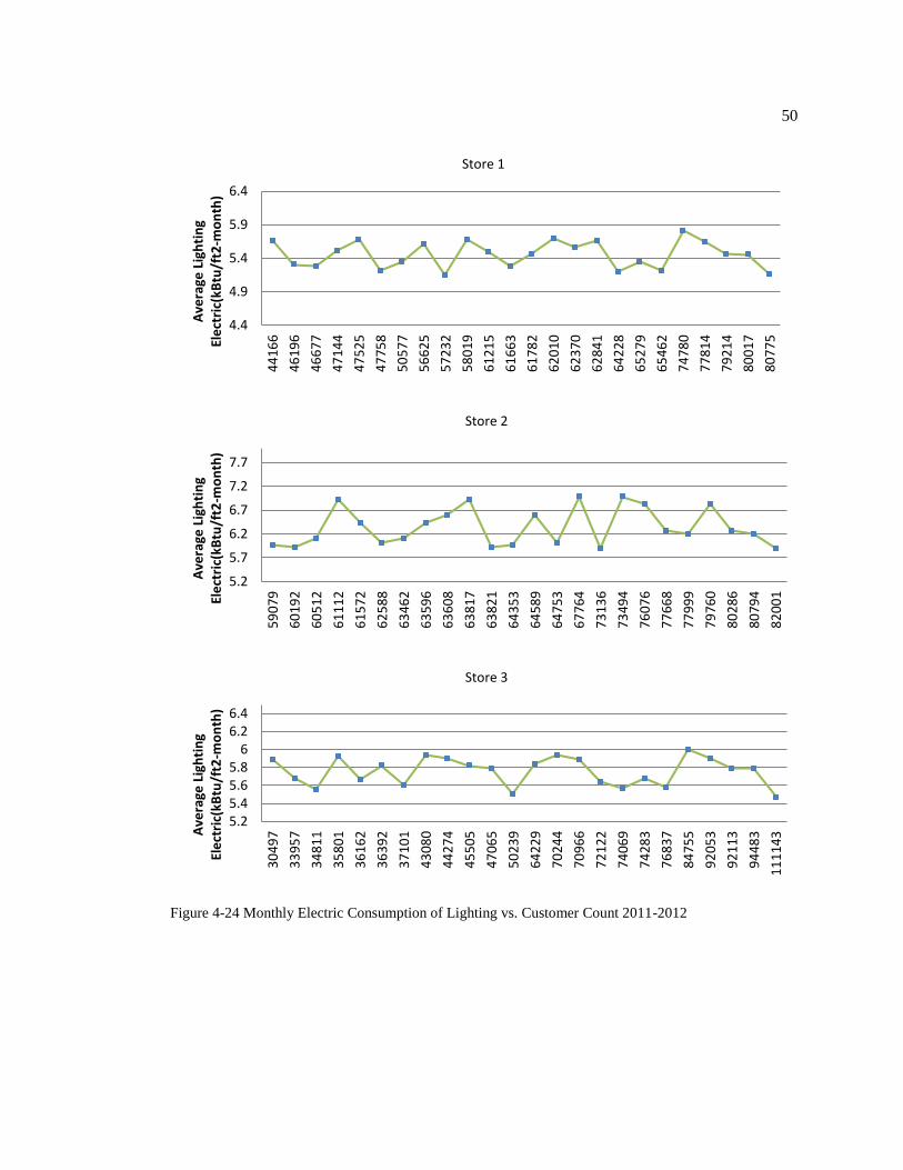
50
Figure 4-24 Monthly Electric Consumption of Lighting vs. Customer Count 2011-2012
4.4
4.9
5.4
5.9
6.4
44
16
6
46
19
6
46
67
7
47
14
4
47
52
5
47
75
8
50
57
7
56
62
5
57
23
2
58
01
9
61
21
5
61
66
3
61
78
2
62
01
0
62
37
0
62
84
1
64
22
8
65
27
9
65
46
2
74
78
0
77
81
4
79
21
4
80
01
7
80
77
5
Ave
rage
Lig
hti
ng
Ele
ctri
c(kB
tu/f
t2-m
on
th)
Store 1
5.2
5.7
6.2
6.7
7.2
7.7
59
07
9
60
19
2
60
51
2
61
11
2
61
57
2
62
58
8
63
46
2
63
59
6
63
60
8
63
81
7
63
82
1
64
35
3
64
58
9
64
75
3
67
76
4
73
13
6
73
49
4
76
07
6
77
66
8
77
99
9
79
76
0
80
28
6
80
79
4
82
00
1
Ave
rage
Lig
hti
ng
Ele
ctri
c(kB
tu/f
t2-m
on
th)
Store 2
5.25.45.65.8
66.26.4
30
49
7
33
95
7
34
81
1
35
80
1
36
16
2
36
39
2
37
10
1
43
08
0
44
27
4
45
50
5
47
06
5
50
23
9
64
22
9
70
24
4
70
96
6
72
12
2
74
06
9
74
28
3
76
83
7
84
75
5
92
05
3
92
11
3
94
48
3
11
11
43A
vera
ge L
igh
tin
g El
ect
ric(
kBtu
/ft2
-mo
nth
)
Store 3

51
Figure 4-25 Refrigeration electric consumption vs. HVAC electric consumption
y = 0.2676x + 2.7436R² = 0.9997
0
1
2
3
4
5
6
0 1 2 3 4 5 6 7 8 9 10
Ave
rage
Re
frig
era
tio
n
Ele
ctri
c(kB
tu/f
t2-m
on
th)
Average HVAC Electric(kBtu/ft2-month)
y = 0.2967x + 2.8793R² = 0.9896
0
1
2
3
4
5
6
0 1 2 3 4 5 6 7 8 9 10
Ave
rage
Re
frig
era
tio
n
Ele
ctri
c(kB
tu/f
t2-m
on
th)
Average HVAC Electric(kBtu/ft2-month)
y = 0.794x + 2.5425R² = 0.9943
0
1
2
3
4
5
6
0 1 2 3 4 5 6
Ave
rage
Re
frig
era
tio
n
Ele
ctri
c(kB
tu/f
t2-m
on
th)
Average HVAC Electric(kBtu/ft2-month)
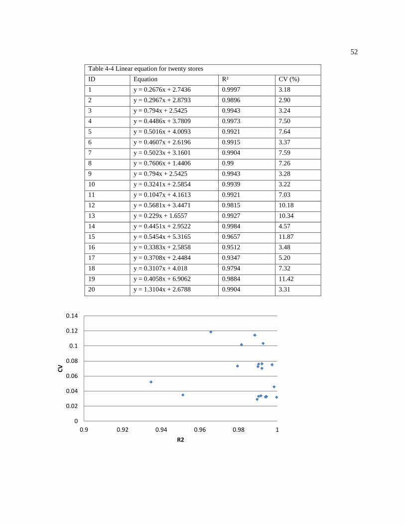
52
Table 4-4 Linear equation for twenty stores
ID Equation R² CV (%)
1 y = 0.2676x + 2.7436 0.9997 3.18
2 y = 0.2967x + 2.8793 0.9896 2.90
3 y = 0.794x + 2.5425 0.9943 3.24
4 y = 0.4486x + 3.7809 0.9973 7.50
5 y = 0.5016x + 4.0093 0.9921 7.64
6 y = 0.4607x + 2.6196 0.9915 3.37
7 y = 0.5023x + 3.1601 0.9904 7.59
8 y = 0.7606x + 1.4406 0.99 7.26
9 y = 0.794x + 2.5425 0.9943 3.28
10 y = 0.3241x + 2.5854 0.9939 3.22
11 y = 0.1047x + 4.1613 0.9921 7.03
12 y = 0.5681x + 3.4471 0.9815 10.18
13 y = 0.229x + 1.6557 0.9927 10.34
14 y = 0.4451x + 2.9522 0.9984 4.57
15 y = 0.5454x + 5.3165 0.9657 11.87
16 y = 0.3383x + 2.5858 0.9512 3.48
17 y = 0.3708x + 2.4484 0.9347 5.20
18 y = 0.3107x + 4.018 0.9794 7.32
19 y = 0.4058x + 6.9062 0.9884 11.42
20 y = 1.3104x + 2.6788 0.9904 3.31
0
0.02
0.04
0.06
0.08
0.1
0.12
0.14
0.9 0.92 0.94 0.96 0.98 1
CV
R2

53
Chapter 5
Demonstration CUSUM Technique for the Monitoring and Targeting (M&T) in
Convenience Stores
The aim of this chapter is to apply a technique for monitoring building end-users energy
consumption change and determine the end-use cause of energy use deviations observed in
whole building. This chapter first introduces CUSUM technique in section 5-1; then section 5-2
demonstrates CUSUM for case studies and section 5-3 illustrates the control chart and CUSUM
interpretation.
5-1 Cumulative Sum of Differences (CUSUM)
M&T turns data on energy use into useful information that can lead to significant
energy and cost savings. This technique is a useful tool to not only track energy use but also to
control it. Building operators, facility managers and “energy champions” have used M&T to
gain insights into their building energy use. M&T helps turn data into valuable, useable
information.
Figure 5-1 illustrates the process applied in M&T, which moves from data to
information and ultimately to results. Instead of just taking measurements, the analysis from
M&T drives the actions that save energy and costs.

54
Figure 5-1 Applied Process in M&T
The regression analysis method produces baseline for whole building and end-use
electricity consumption. The baseline can be used to predict energy use in a period for a
specified set of conditions described by the outdoor dry bulb temperatures. Future use can be
compared with the prediction to determine whether energy use is higher or lower than predicted.
The difference in energy use between actual and target is calculated for each period and added
together, creating a “running total.” This is referred to as the CUSUM, or Cumulative Sum, of
the differences. The CUSUM is also referred to as the cumulative savings total. Trends in the
CUSUM graph indicate consumption patterns. The case studies presented in this study
demonstrate the use of the CUSUM graph. According to one user of M&T, The CUSUM graph
really tells you a story (Natural Resources Canada, 2007). The CUSUM process step by step is
as a below:
1. Get the baseline;
2. Derive the equation of the baseline;
3. Calculate the expected energy consumption based on the equation;
4. Calculate the difference between actual and calculated energy use;
5. Compute CUSUM;

55
6. Plot the CUSUM graph over the time.
Associated CUKSUM M&T analysis tool allows facility managers to immediately
determine the end-use cause of energy use deviations observed in the energy use CUKSUM
reporting.
5-2 Demonstration CUSUM for the Case Studies
Table 5-1 shows identification information of the convenience store for which the data
is displayed. This has a gasoline fueling station and is located in Virginia.
Table 5-1 Store Identification
Area (ft2) 6090
Open Date 6/6/2008
Location Virginia State
Type with Fuel Station
Annual Electric Consumption (kWh) 591,520
Annual Natural Gas Consumption (therms) 1,288
Average Customer Count per year 697,00
Figures 5-2, 5-3, 5-4 and 5-5 show baseline of whole building, refrigeration, HVAC and
lighting electric consumption vs. average daily outdoor air temperature respectively which
include the lines of 95% Confidence intervals and 95% of Prediction intervals. Confidence
intervals tell you about how well you have determined the baseline. Prediction intervals tell you
where you can expect to see the next data point.
Prediction intervals must account for both the uncertainty in knowing the value of the
population mean, plus data scatter. So a prediction interval is always wider than a confidence
interval (Graph Pad, 2007).
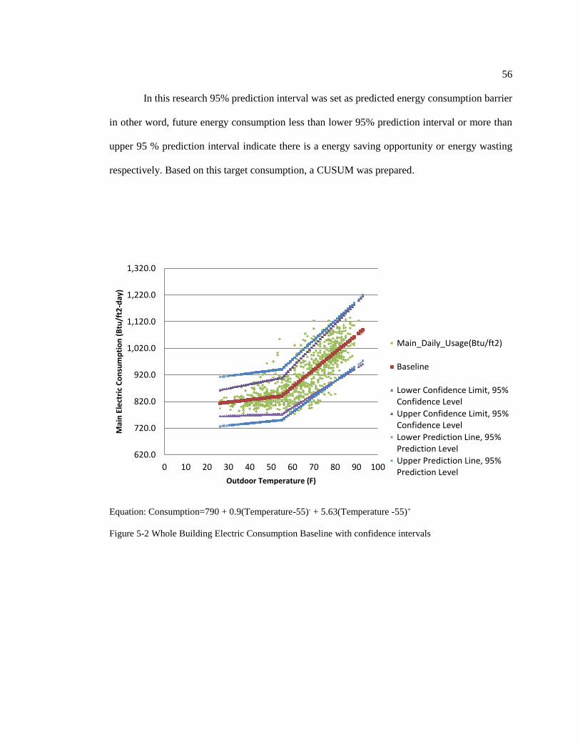
56
In this research 95% prediction interval was set as predicted energy consumption barrier
in other word, future energy consumption less than lower 95% prediction interval or more than
upper 95 % prediction interval indicate there is a energy saving opportunity or energy wasting
respectively. Based on this target consumption, a CUSUM was prepared.
Equation: Consumption=790 + 0.9(Temperature-55)- + 5.63(Temperature -55)+
Figure 5-2 Whole Building Electric Consumption Baseline with confidence intervals
620.0
720.0
820.0
920.0
1,020.0
1,120.0
1,220.0
1,320.0
0 10 20 30 40 50 60 70 80 90 100
Mai
n E
lect
ric
Co
nsu
mp
tio
n (
Btu
/ft2
-day
)
Outdoor Temperature (F)
Main_Daily_Usage(Btu/ft2)
Baseline
Lower Confidence Limit, 95%Confidence Level
Upper Confidence Limit, 95%Confidence Level
Lower Prediction Line, 95%Prediction Level
Upper Prediction Line, 95%Prediction Level
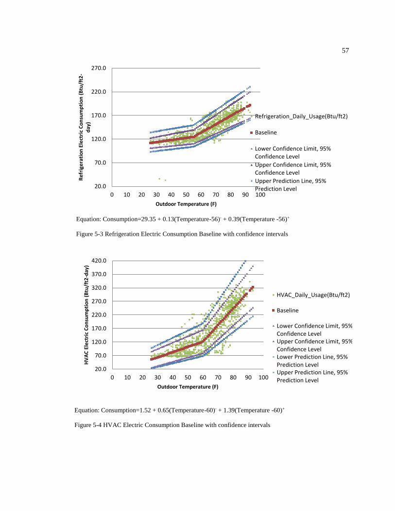
57
Equation: Consumption=29.35 + 0.13(Temperature-56)- + 0.39(Temperature -56)+
Figure 5-3 Refrigeration Electric Consumption Baseline with confidence intervals
Equation: Consumption=1.52 + 0.65(Temperature-60)- + 1.39(Temperature -60)+
Figure 5-4 HVAC Electric Consumption Baseline with confidence intervals
20.0
70.0
120.0
170.0
220.0
270.0
0 10 20 30 40 50 60 70 80 90 100
Re
frig
era
tio
n E
lect
ric
Co
nsu
mp
tio
n (
Btu
/ft2
-d
ay)
Outdoor Temperature (F)
Refrigeration_Daily_Usage(Btu/ft2)
Baseline
Lower Confidence Limit, 95%Confidence Level
Upper Confidence Limit, 95%Confidence Level
Upper Prediction Line, 95%Prediction Level
20.0
70.0
120.0
170.0
220.0
270.0
320.0
370.0
420.0
0 10 20 30 40 50 60 70 80 90 100
HV
AC
Ele
ctri
c C
on
sum
pti
on
(B
tu/f
t2-d
ay)
Outdoor Temperature (F)
HVAC_Daily_Usage(Btu/ft2)
Baseline
Lower Confidence Limit, 95%Confidence LevelUpper Confidence Limit, 95%Confidence LevelLower Prediction Line, 95%Prediction LevelUpper Prediction Line, 95%Prediction Level

58
Equation: Consumption=63.58 - 0.17 (Temperature-66)- + 0.06(Temperature -66)+
Figure 5-5 Lighting Electric Consumption Baseline with confidence intervals
After calculate the expected energy consumption based on the equation and calculate
the difference between actual and calculated energy use CUSUM was calculated. Figure 5-6
presents CUSUM for Whole building, Refrigeration, HVAC and Lighting of studied building
during 2011-2012 and figures 5-7 shows CUSUM for Whole building, Refrigeration, HVAC
and Lighting of studied building for October 2012, which shows more details.
150.0
160.0
170.0
180.0
190.0
200.0
210.0
220.0
0 10 20 30 40 50 60 70 80 90 100
Ligh
tin
g El
ect
ric
Co
nsu
mp
tio
n (
Btu
/ft2
-day
)
Outdoor Temperature (F)
Lighting_Daily_Usage(Btu/ft2)
Baseline
Lower Confidence Limit, 95%Confidence LevelUpper Confidence Limit, 95%Confidence LevelLower Prediction Line, 95%Prediction LevelUpper Prediction Line, 95%Prediction Level
-4.00
-3.00
-2.00
-1.00
0.00
1.00
2.00
Jan
Feb
Mar
Ap
r
May Jun
Jul
Au
g
Sep
Oct
No
v
De
c
Jan
Feb
Mar
Ap
r
May Jun
Jul
Au
g
Sep
Oct
No
v
De
cCU
SUM
(kB
tu/f
t2-m
on
th)
Whole Building

59
Figure 5-6 CUSUM for 201-2012
-1.00-0.80-0.60-0.40-0.200.000.20
Jan
Feb
Mar
Ap
r
May Jun
Jul
Au
g
Sep
Oct
No
v
De
c
Jan
Feb
Mar
Ap
r
May Jun
Jul
Au
g
Sep
Oct
No
v
De
c
CU
SUM
(kB
tu/f
t2-m
on
th)
Refrigeration
-4.00
-3.00
-2.00
-1.00
0.00
1.00
Jan
Feb
Mar
Ap
r
May Jun
Jul
Au
g
Sep
Oct
No
v
De
c
Jan
Feb
Mar
Ap
r
May Jun
Jul
Au
g
Sep
Oct
No
v
De
c
CU
SUM
(kB
tu/f
t2-m
on
th)
HVAC
-0.20
0.00
0.20
0.40
0.60
0.80
Jan
Feb
Mar
Ap
r
May Jun
Jul
Au
g
Sep
Oct
No
v
De
c
Jan
Feb
Mar
Ap
r
May Jun
Jul
Au
g
Sep
Oct
No
v
De
c
CU
SUM
(kB
tu/f
t2-m
on
th)
Lighting

60
Figure 5-7 CUSUM for October 2012
-0.50-0.40-0.30-0.20-0.100.000.10
CU
SUM
(kB
tu/f
t2-m
on
th)
Whole Building
-0.15
-0.10
-0.05
0.00
CU
SUM
(kB
tu/f
t2-m
on
th)
Refrigeration
-0.40
-0.30
-0.20
-0.10
0.00
CU
SUM
(kB
tu/f
t2-m
on
th)
HVAC
-0.06
-0.04
-0.02
0.00
0.02
CU
SUM
(kB
tu/f
t2-m
on
th)
Lighting
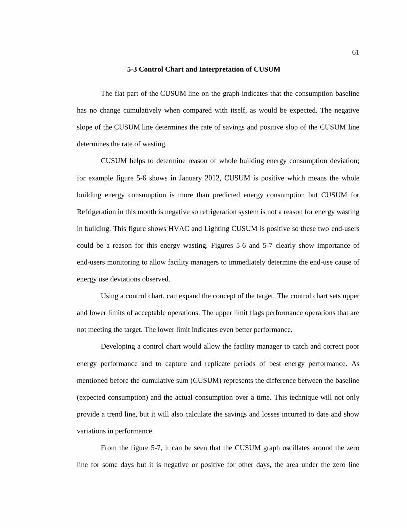
61
5-3 Control Chart and Interpretation of CUSUM
The flat part of the CUSUM line on the graph indicates that the consumption baseline
has no change cumulatively when compared with itself, as would be expected. The negative
slope of the CUSUM line determines the rate of savings and positive slop of the CUSUM line
determines the rate of wasting.
CUSUM helps to determine reason of whole building energy consumption deviation;
for example figure 5-6 shows in January 2012, CUSUM is positive which means the whole
building energy consumption is more than predicted energy consumption but CUSUM for
Refrigeration in this month is negative so refrigeration system is not a reason for energy wasting
in building. This figure shows HVAC and Lighting CUSUM is positive so these two end-users
could be a reason for this energy wasting. Figures 5-6 and 5-7 clearly show importance of
end-users monitoring to allow facility managers to immediately determine the end-use cause of
energy use deviations observed.
Using a control chart, can expand the concept of the target. The control chart sets upper
and lower limits of acceptable operations. The upper limit flags performance operations that are
not meeting the target. The lower limit indicates even better performance.
Developing a control chart would allow the facility manager to catch and correct poor
energy performance and to capture and replicate periods of best energy performance. As
mentioned before the cumulative sum (CUSUM) represents the difference between the baseline
(expected consumption) and the actual consumption over a time. This technique will not only
provide a trend line, but it will also calculate the savings and losses incurred to date and show
variations in performance.
From the figure 5-7, it can be seen that the CUSUM graph oscillates around the zero
line for some days but it is negative or positive for other days, the area under the zero line

62
shows saved amount of energy and the area above zero line shows amount of lost energy during
the time. Figure 5-8 shows amount of used energy more or less than expected. The control chart
in figure 5-8 shows the difference each day between actual and predicted use; target lines were
extracted from 95% prediction level, which was shown in figure 5-2 to 5-5. According to figure
5-8 day 24 is out of control, also day 22 would be a good day to ask, “What did we do well?”
This method is applicable to calculate energy saving in post-retrofit period. Regarding
calculating post-retrofit energy saving, we should follow below steps:
1. Get the pre-retrofit baseline (consider at least 1 year data);
2. Derive the equation of the pre-retrofit baseline;
3. Calculate the expected energy consumption based on the pre-retrofit baseline equation;
4. Calculate the difference between energy consumption in post-retrofit and expected
energy consumption in pre-retrofit (use pre-retrofit equation);
5. Compute CUSUM;
6. Plot the CUSUM graph over the time;
7. Calculate saving energy.
Note with considering capital cost of retrofit and amount of saved energy we can
estimate payback period for retrofit and define is the retrofit case financially reasonable or not.
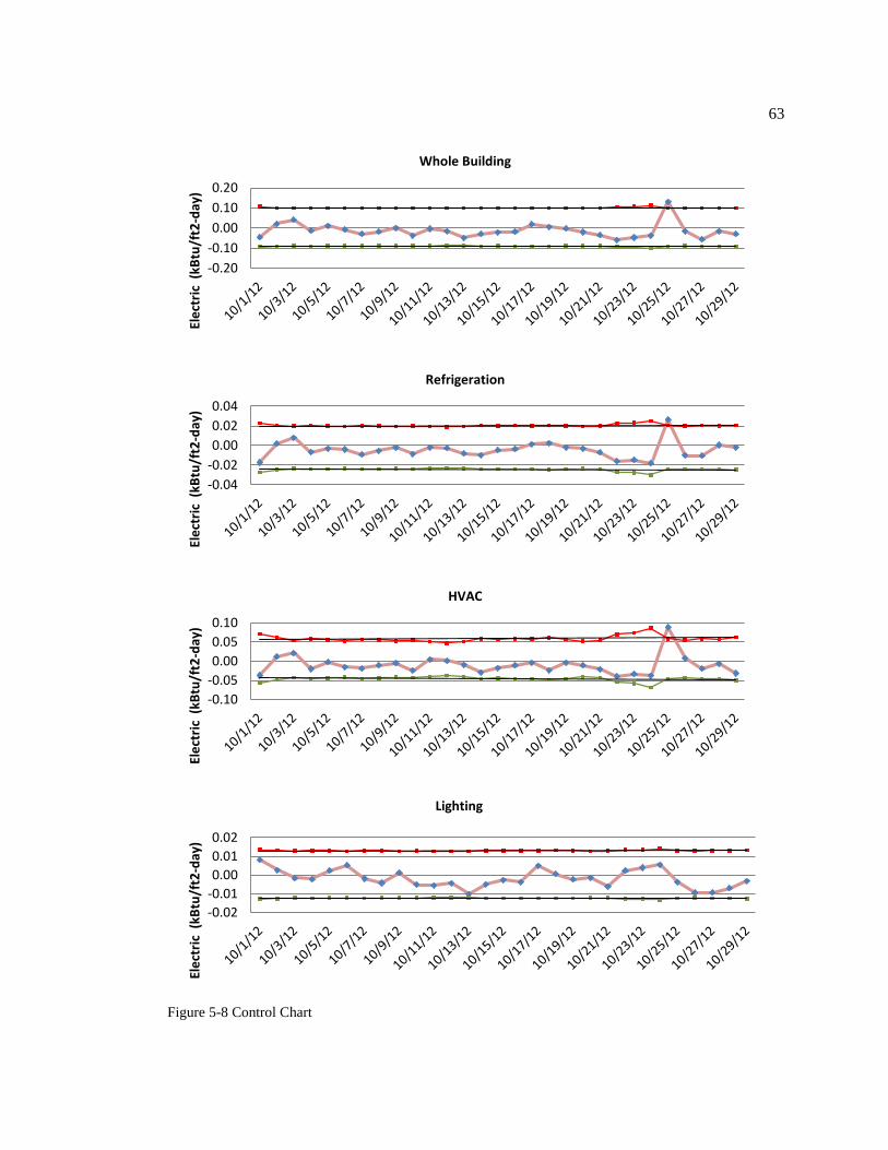
63
Figure 5-8 Control Chart
-0.20
-0.10
0.00
0.10
0.20El
ect
ric
(kB
tu/f
t2-d
ay)
Whole Building
-0.04
-0.02
0.00
0.02
0.04
Ele
ctri
c (
kBtu
/ft2
-day
)
Refrigeration
-0.10
-0.05
0.00
0.05
0.10
Ele
ctri
c (
kBtu
/ft2
-day
)
HVAC
-0.02
-0.01
0.00
0.01
0.02
Ele
ctri
c (
kBtu
/ft2
-day
)
Lighting
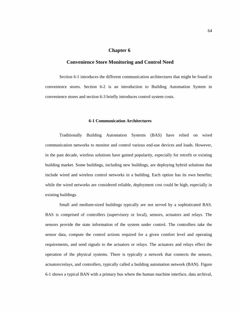
64
Chapter 6
Convenience Store Monitoring and Control Need
Section 6-1 introduces the different communication architectures that might be found in
convenience stores. Section 6-2 is an introduction to Building Automation System in
convenience stores and section 6-3 briefly introduces control system costs.
6-1 Communication Architectures
Traditionally Building Automation Systems (BAS) have relied on wired
communication networks to monitor and control various end-use devices and loads. However,
in the past decade, wireless solutions have gained popularity, especially for retrofit or existing
building market. Some buildings, including new buildings, are deploying hybrid solutions that
include wired and wireless control networks in a building. Each option has its own benefits;
while the wired networks are considered reliable, deployment cost could be high, especially in
existing buildings.
Small and medium-sized buildings typically are not served by a sophisticated BAS.
BAS is comprised of controllers (supervisory or local), sensors, actuators and relays. The
sensors provide the state information of the system under control. The controllers take the
sensor data, compute the control actions required for a given comfort level and operating
requirements, and send signals to the actuators or relays. The actuators and relays effect the
operation of the physical systems. There is typically a network that connects the sensors,
actuators/relays, and controllers, typically called a building automation network (BAN). Figure
6-1 shows a typical BAN with a primary bus where the human machine interface, data archival,

65
and other application, which the building operators interact with, reside. The secondary bus
typically has the sensors and actuators/relays that interact with the physical systems
(conditioned space, and building HVAC and lighting equipment).
Figure 6-1 Typical architecture of a BAN
Most BANs serving small or medium-sized buildings can be classified into three
different kinds – wired, wireless, and hybrid.
Wired Network: A significant portion of the current BASs relies on wired
communication networks. While wired networks are considered reliable, deployment cost is
significant. In the secondary bus, the location of the sensors typically is dictated by the location
of the controllers and access limitations (usually distance, obstructions and first costs) rendering

66
sub-optimal control of the thermal environment. Typical wired medium includes Serial link,
Ethernet, Optical, and power line communications.
Serial links are typically point-to-point communication links used in BAN with limits
on the length up to 50m per link. There are several different implementations of the serial link
and associated protocols used by the BANs. Electronic Industries Association (EIA)
standardized the electrical characteristics and physical layer requirements in EIA-485 standard.
The link can be established as two-wire-twisted pair (half duplex), three-wire-twisted pair (half
duplex with differential signaling), and four-wire-twisted pair (full duplex). Proprietary
implementations of this protocol exist; for example, N2 bus is a technology developed using
EIA-485 by Johnson Controls (JCI 1999) to connect various controllers to a master/supervisory
controller (Figure 6-2). Typical serial links operate at a maximum rate of 115 kbps. However,
recently optical layers are being used for the serial links necessitating optical modems on either
end of the bus for specific applications.
Figure 6-2 Example of Cascaded Devices using N2 Serial Bus

67
Ethernet is a popular option for BAN because of its ubiquitous use in buildings and ease
of network management. The ease of installation and configuration of Ethernet is making it an
increasingly accepted choice among vendors and buildings managers. The use of Ethernet
enables the use of Internet protocol (IP) on the devices connected within buildings and provides
unique addressing and access (remote) schemes for sensors, actuators, and controllers.
LonWorks, which provide a data link layer and physical signaling for BANs, has adapters to
connect between serial links and Ethernet communications. Similarly BACnet protocol provides
interface to IP communications for managing devices on BAN.
The Power line carrier (PLC) approach is based on converting digital data to radio
frequencies and sending the signals down the electric power lines. The technology is similar to
broadband cable except the power lines are used instead of a coaxial cable. The technology is
convenient in that the service is available anywhere there are power lines without running
additional cables. However, there are huge drawbacks using this mode of communication for
BAN. Power lines are typically noisy with effective communication bandwidth limited to 10
kbps. Routing data through existing circuits requires careful planning and installation to
eliminate network disconnections. In addition, provision for transformers in the electrical
system must be made, or the signals will stop at the transformer. This provision usually is some
type of “bypass” around the transformer. Because of increased safety constraints related to
worker safety when exposed to power, this mode of communications is becoming less popular.
Wireless Network: Wireless sensor network (WSN) provides an attractive retro-
commissioning opportunity in existing buildings. Wide variety of wireless networks exist that
can be used to instrument buildings. Figure 6-3 shows the options in wireless networks. The x-
axis represents the data rate and the y-axis represents the power consumption and
cost/complexity.

68
Figure 6-3 Wireless Landscape
Hybrid Wired-Wireless Networks: While wireless sensors provide clear advantages
over wireless networks for building automation, there are several buildings with limited wired
infrastructure for sensing and actuation of building subsystems. One attractive approach is to
utilize the existing network and use wireless sensors and actuators to provide additional
monitoring and control of building subsystems. Interoperability of wired and wireless networks
can be achieved in several ways. Two significant implementations are: (1) application-level
interoperability, and (2) link-level interoperability. Application-level interoperability includes a
central server that can communicate with both the networks and exchanges data (via a database)
to different applications for building management. Link-level interoperability includes a
gateway that can communicate with the wireless network and translates the data to the existing
buildings automation protocol (BACnet, LonWorks), as shown in figure 6-4 and figure 6-5.
Using the gateway the wireless network points can be seen as, for example, LonWorks points
providing an easy way to manage a network of wireless sensors. Hybrid networks have the
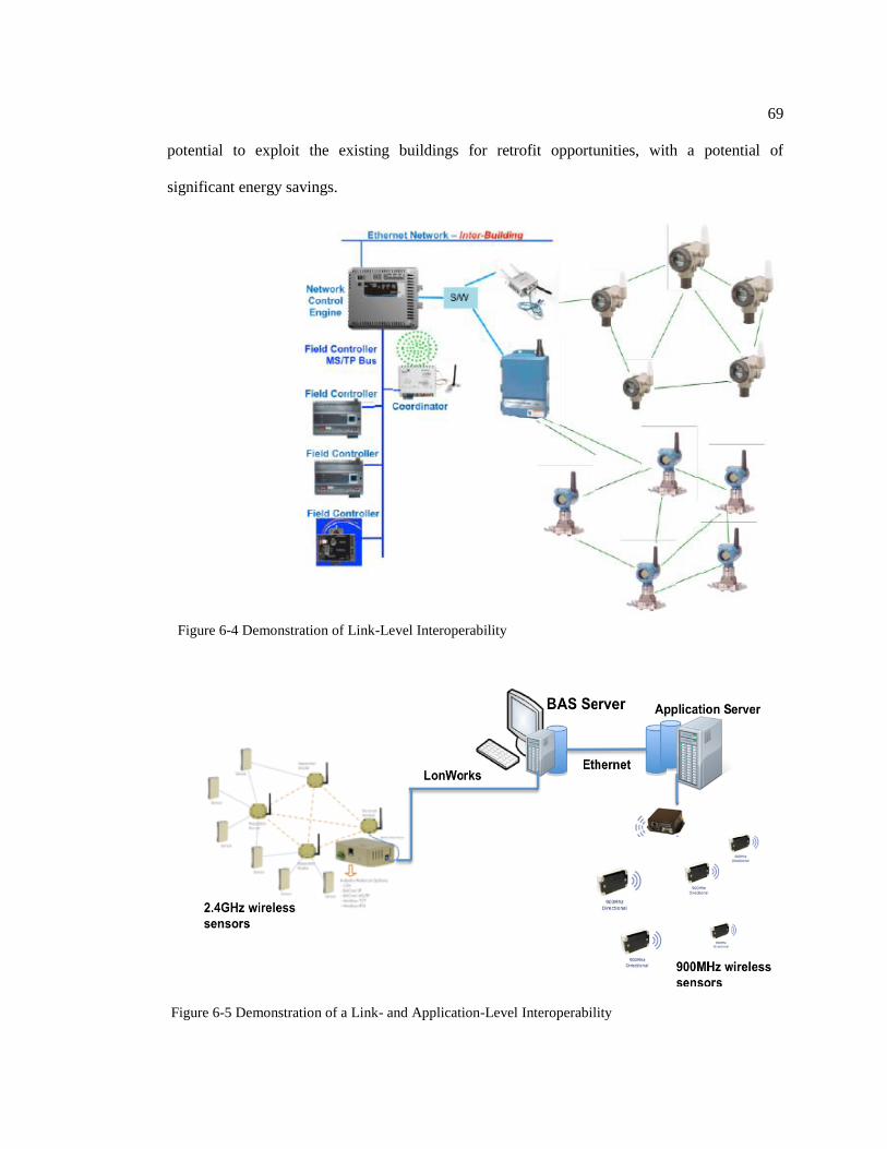
69
potential to exploit the existing buildings for retrofit opportunities, with a potential of
significant energy savings.
Figure 6-4 Demonstration of Link-Level Interoperability
Figure 6-5 Demonstration of a Link- and Application-Level Interoperability
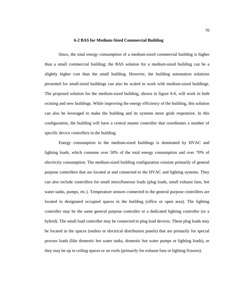
70
6-2 BAS for Medium-Sized Commercial Building
Since, the total energy consumption of a medium-sized commercial building is higher
than a small commercial building; the BAS solution for a medium-sized building can be a
slightly higher cost than the small building. However, the building automation solutions
presented for small-sized buildings can also be scaled to work with medium-sized buildings.
The proposed solution for the medium-sized building, shown in figure 6-6, will work in both
existing and new buildings. While improving the energy efficiency of the building, this solution
can also be leveraged to make the building and its systems more grids responsive. In this
configuration, the building will have a central master controller that coordinates a number of
specific device controllers in the building.
Energy consumption in the medium-sized buildings is dominated by HVAC and
lighting loads, which consume over 50% of the total energy consumption and over 70% of
electricity consumption. The medium-sized building configuration consists primarily of general
purpose controllers that are located at and connected to the HVAC and lighting systems. They
can also include controllers for small miscellaneous loads (plug loads, small exhaust fans, hot
water tanks, pumps, etc.). Temperature sensors connected to the general purpose controllers are
located in designated occupied spaces in the building (office or open area). The lighting
controller may be the same general purpose controller or a dedicated lighting controller (or a
hybrid). The small load controller may be connected to plug load devices. These plug loads may
be located in the spaces (outlets or electrical distribution panels) that are primarily for special
process loads (like domestic hot water tanks, domestic hot water pumps or lighting loads), or
they may be up in ceiling spaces or on roofs (primarily for exhaust fans or lighting fixtures).

71
Figure 6-6 BASs with Local Control and Configuration and Local or Remote Monitoring for Medium-
Sized Buildings
The communication between individual controllers and the master controller and
between sensors and controllers can be wired or wireless. Individual controllers do not need to
communicate to the Cloud service directly. Access to external information in the controllers is
primarily through the master controller. Monitoring can either be via local or remote monitoring
(web page, Internet connection – wired or wirelessly). Local monitoring, configuration and
analysis (data and alarm management) is the recommended option for medium-sized buildings.
Monitoring capabilities greatly assist in ensuring persistence and sustainability of energy
savings and proper, efficient equipment operations. This assurance comes primarily from
reliable alarm, data management and actionable intelligence creation capabilities.
Control functions are distributed primarily amongst the programmable general purpose
controllers, but there will (of necessity) be some “global” functions that come from a local, on-
72
site master controller. This type of control may be viewed as a “master/slave” or “supervisory”
management service that includes site configuration of individual controllers, as well as alarm
and data management (local data storage, etc.). Global functions may also include (but are not
necessarily limited to) alarm management (alarm monitoring and alarm notification), data
management (trending, storage and retrieval), equipment scheduling, holiday scheduling and
time synchronization actions. All of these control devices shall be connected to a common
communications network (wired or wireless or both) inside the building. Communications to all
controllers should be based on an open standard. When specifying such a system,
it is always important to fully document the installation and startup of all
hardware/software functions so it will be easy to implement and troubleshoot (startup and
persistence).
This configuration will generally be dealing with a significant number of HVAC
systems (more than five), a number of lighting controllers and other special purpose load
controllers. In existing medium-sized commercial buildings, when lighting control is
implemented, lighting automation panels, also called lighting relay panels or lighting control
panels are a common means of implementing schedules. Panel-based controls may also support
the integration of occupancy and photo-sensors for sensor-based on-off control. Panel-based
controllers may be integrated with BASs (e.g., via BACnet) or may be networked with one
another using proprietary protocols. Common lighting control architectures are detailed in
Appendix B, including schematic diagrams.
The HVAC systems can include rooftop configurations (multi-stage heating and
cooling) that may also include economizer functions (integrated or standalone), split systems
(indoor fan unit with outdoor condenser), larger air handling units (primarily packaged), zone
terminal boxes or zone HVAC systems (like fan coils or induction boxes, etc.) and potentially

73
small chillers and hot water boilers with dedicated pumping systems. The configuration may be
dealing with a few small load controllers.
Programmable general purpose controllers that support multiple configurations (heat
pump, multi-stage heating and cooling, with or without economizer integration, terminal boxes,
air handlers, etc.) over multiple product offerings that are designed for only one type of HVAC
system are probably not realistic for the size and potential complexity of medium buildings,
especially when designed with multiple and varying HVAC systems. Determination of giving
preference to controllers that support multiple configurations over multiple product offerings
(because of varied HVAC systems that are not conducive to one controller option) will be
market and building system driven.
Configuration of all general purpose control parameters shall be configured from a local
workstation or a local laptop computer connection to the general purpose controller. Remote
access via web access/web page service into the local controller is also encouraged, to provide
for remote service and troubleshooting.
Different levels of program access shall be required for each general purpose controller.
Basic access shall be provided to allow for local occupant overrides and other non-critical
functions. Higher level access (via proper password access) shall be provided for
service/maintenance personnel or other designated staff. This higher level access shall include
access for schedule changes and equipment protection parameters (minimum on-off short-cycle
parameters and/or similar functions).
Remote configuration and monitoring may be provided for all controllers. The
programmable controller may have a bypass/override feature that enables testing basic HVAC
equipment functions. Analytics and actionable intelligence can be created, either locally or
remotely or both. This includes tracking HVAC equipment performance issues such as dirty
filters, hours of heating and cooling operations with local notification for maintenance
74
inspections and can include storage of time-stamped alarms (high/low temperatures, etc.). The
detailed capabilities of the general purpose HVAC controller, load controller and lighting
controller are given in the next section (DOE, 2012)
6-3 System Costs
The cost of this system is varying widely for a number of reasons: equipment
specifications and capabilities, existing infrastructure, site-specific design conditions, local cost
factors, etc. This report does not present specific cost estimates. Instead, it will identify the main
cost components that should be addressed when developing a cost estimate.
The system cost estimate can be separated into three main categories: capital, labor, and
recurring costs. Capital cost refers to the cost of the meters and all materials required to support
their installation:
Meter purchase cost, the purchase price depends on the required features selected such
as accuracy, memory, and mounting.
Ancillary devices, electric meters require current transformers (CTs), potential
transformers (PTs) and safety switches. These devices may be built into the meter or can be
specified separately. Natural gas and steam meters may require filters or strainers, temperature
and pressure compensators, flow straightness, and straight pipe runs. These devices affect
design, practicality, cost, and may influence the type of meter that can be specified for a given
application.
Communications module, there are a number of types of communication
methodologies that can be incorporated into meters. Communication may be wired or wireless,
analog or digital, one-way or two-way, periodic or continuous. The meter’s communication

75
module may include a handheld reader communicator, telephone modem, cellular modem, radio
transceiver, power line carrier modem, Ethernet modem, Wi-Fi, hard wire (RS232 or RS485), or
supervisory control and data acquisition (SCADA) interface. Communications modules are
usually specified with the meter.
Miscellaneous supplies, small compared to other hardware line-item costs,
miscellaneous supplies include items such as wire, conduit, and junction boxes necessary to
complete the installation. Also, consider the power supply to the meter and data transmission
system.
Labor covers the time involved for a crew to install all of the hardware, connect the
communications module, perform operational testing, and inspect the functionality of the
metering system. Examples of variables in the labor costs include the type of meter being
installed (utility being metered and if the meter is intrusive or non-intrusive), service shutdowns
that may need to be accomplished during off-hours, and trenching requirements for running
cable.
Recurring costs: Recurring costs are planned regular costs that support the ongoing
operation of the meter/metering system.

76
Chapter 7
Conclusions and Recommendations for Future Studies
Based on the findings of this dissertation, this study summarizes the Conclusions in
Section 7.1 and recommendations for the future studies in 7.2.
7-1 Conclusions
The main objective of this research was to establish inverse modeling analysis tools to
enable continuous efficiency improvement loop. The necessary tools and steps were identifying
the store specific energy use baselines and analysis of ongoing, operational data deviations from
the baseline using the Cumulative Sum (CUSUM) method. The results indicate that the
similarly designed stores exhibit qualitatively similar baseline with changes in ambient weather
conditions with respect to whole building energy use and subsystem energy uses. However, the
quantitative levels of energy use as well as the changes in energy use with changes in ambient
temperature are store specific, even for stores in close physical proximity. The energy use
patterns are quite reproducible for a specific store and deviations are observed to occur only
when significant changes in site equipment performance or building envelope changes occur.
In this study, it was shown identifying baseline with simple Excel spreadsheet
functional capability is easier than using Inverse Modeling Toolkit (IMT) and has comparable
accuracy.
The results of this study present more accurate baseline models with using daily energy
consumption as dependent variable instead of monthly bill tracking.
One of the results in this study shows the lighting electric consumption is not under the
effect of outdoor temperature variation.

77
The results show monthly customer count is not enough data to show building and end-
users electric consumption relationship with customer’s number.
One of the most important finding was that there is a strong linear relationship between
HVAC and Refrigeration electric consumption and both have strong ambient temperature
dependencies. It is suspected that the time – of – day customer count data is a similarly
important parameter for energy use predications, but that data was not available for this study.
The most important finding in this study presents a method to detect building energy
trend cause by looking at building end-users CUSUM report, which allows facility managers to
immediately determine the end-use cause.
The proposed methodology can be used for retrofit savings analysis.
7.2 Recommendations for Future Studies
In this study, developing a methodology to audit, monitor and target energy use in end-
uses of convenience stores to enable continues efficiency improvement loop was the main
objective.
This study considered outdoor dry bulb temperature as only dependent energy
consumption driver for convenience stores end-users, Refrigerating, HVAC and lighting. Future
studies can investigate effect of other parameter such as internal load, internal condition, time-
of-day customer count, building conditions such as elevation, orientation.
Electricity consumption amounts by end-uses meter were the dependent values. Future
studies may want to consider conditions such as equipment efficiency, age as well as
economizer utilization influences on energy consumption.

78
Although this study focused on specific convenience stores , this technique could be
automated and used in continuous energy monitoring of an entire fleet of similar, high energy
utilization commercial building types.
In this study weather, data was characterized based on the outdoor Daily Mean
Temperature (DMT). A comparison between DMT and cooling and heating degree days
(CDDs), (HDDs) results accuracy would be useful.
There is a lake of software for conduct this process automatically, which could provide
feedback for the existing city benchmarking to entire fleet of similar, high energy utilization
commercial building types.
A study on relationship between HVAC and refrigeration electric consumption as a
function of time-0f-day customer count and ambient temperature as independent variables is
highly recommended.

79
Bibliography
- A. Mahdavi, Mohammadi, A., Kabir, E., Lambeva, L., 2008, Occupants' operation of lighting and
shading systems in office buildings, Journal of Building Performance Simulation, 1 (1) 57-65.
- Askounis D.T.H., Psarras J.,1998, Information system for monitoring and targeting (M&T)
of energy consumption in breweries. Energy 1998; 23(5):413–9.
- ASHRAE, 2002, Guideline 14 Measurement of Energy and Demand Savings.
- ASHRAE, 2009, ASHRAE Handbook of Fundamentals.
- ASHRAE, 2010, Standard 90.1-2010, Energy Standard for Buildings except Low Rise
Residential Buildings.
- ASHRAE, 2014, Guideline 13 Specifying Building Automation Systems.
- Beggs, C., 2002, Energy: Management, supply and conservation. Woburn, MA: Butterworth-
Heinemann.
- Bonneville Power Administration (BPA), 2012), Monitoring, Targeting and Reporting (MT&R)
Reference Guide - Revision 3. Retrieved from: bpa.gov
- Buildings, Office of Energy Efficiency & Renewable Energy,
http://energy.gov/eere/efficiency/buildings (Access: Feb.2016).
- Carbon Trust, 2010, CTG 008 Monitoring and targeting guide.
- Carbon Trust, 1998, Monitoring and Targeting in Large Companies. Good Practice Guide 112,
Oxford, United Kingdom: Carbon Trust.
- Days, A.R. and Karayiannis, T.G., 1999, Identification of the uncertainties in degree -day- based
energy estimates. Building Services Engineering Research and Technology, Vol. 20:165.
- D. Lindelöf, N. Morel, 2006, A field investigation of the intermediate light switching by users,
Energ Buildings, 38 (7) 790-801.

80
- Effinger, J., Effinger, M., Friedman, H., 2011, Case studies in using interval data energy models
for savings verification: lessons from the grocery sector, ESL-IC-11-10-15.
- Eger, B. and Kissock, K.,2007, “Understanding Industrial Energy Use through Sliding Regression
Analysis”, Energy in Industry, July 24-27.
- Energy Efficiency Accessible link: http://energy.gov/science-innovation/energy-efficiency
(Access: Feb.2016).
- Energy Monitoring and Targeting,
http://www.energy.gov.za/EEE/Projects/Industrial%20Energy%20Management/IEM%20Trainin
g/Modules/IEMTCModule7_final.pdf (Access: Feb.2016).
- Energy Smart Industrial BPA Energy Efficiency, 2015, Monitoring, Targeting and Reporting
(MT&R) Reference Guide
- Energy Smart Tips for Convenience Stores,
http://smartenergy.illinois.edu/pdf/Convenience%20Store%20Niche%20FINAL%20-
%2005.02.2011.pdf (Access: 2016).
- EnergyStar , Department of Energy, What is energy use intensity (EUI)?
http://www.energystar.gov (Access: Feb.2016).
- Graph Pad Software, Frequently Asked Questions
http://www.graphpad.com/support/faqid/1506/ (Access: Feb.2016).
- Guillermo Ignacio León Orellana,2014, “Development of a Methodology for Auditing,
Monitoring and Targeting Energy Use in Convenience Stores”, Master Thesis, ThePennsylvania
State University.
- Haberl, J.A., T. Agami Reddy, and J. Elleson. 1997. “Determining Long-Term Performance of
Cool Storage Systems from Short-Term Tests.” ASHRAE Reseasrch Project 1004.
- Harris P., 1989, Energy Monitoring and Target Setting Using CUSUM. Cambridge:
Cheriton Technologies Publication.
- Independent Statistics & Analysis U.S. Energy Information Administration, Commercial
Buildings Energy Consumption Survey
http://www.eia.gov/consumption/commercial/reports/2012/preliminary/ (Access: Feb.2016).

81
- Institute for Digital Research and Education (IDRE), 2013, what is the coefficient of
http://www.ats.ucla.edu/stat/mult_pkg/faq/general/coefficient_of_variation.htm(Access:
Feb.2016).
- Katipamula, S., Reddy, T.A. and Claridge, D.E.,1998, Multivariate Regression Modeling.
Journal of Solar Energy Engineering, vol. 120, P.177-184.
- Kissock, J. Kelly, Jeff S. Haberl, and David E. Claridge,2002, Development of a Toolkit
for Calculating Linear, Change-point Linear and Multiple-Linear Inverse Building Energy
Analysis Models. Final Report for ASHRAE Research Project, No. 1050-RP. Energy Systems
Laboratory.
- Levermore, G.J., 2000, Building Energy Management Systems. New York, NY: E&FN Spoon.
- Mohammad Heidarinejad, 2014, “Relative Significance of Heat Transfer Processes to Quantify
Tradeoffs Between Complexity and Accuracy of Energy Simulations With a Building Energy Use
Patterns Classification”, PhD Thesis, The Pennsylvania State University.
- NACS, the Association for Convenience & Fuel Retailing
http://www.nacsonline.com/Research/FactSheets/scopeofindustry/pages/convenience.aspx
(Access: Feb.2016).
- Natural Resource Canada, Monitoring and Targeting Techniques in Buildings,
http://www.nrcan.gc.ca/energy/publications/efficiency/buildings/5957 (Access: Feb.2016).
- Reddy, T. Agami, and David E. Claridge, 2000, “Uncertainty of ‘Measured’ Energy Savings from
Statistical Baseline Models.” HVAC&R Research 6 (1): 3–20.
- Parichehr Salimifard, 2014, “Comparison of Part Load Model Prediction of Commercial Office
Subsystem Energy Consumption with Sub-Metered Data”. Master Thesis, The Pennsylvania State
University.
- PDHonline Course M196 (4 PDH), 2012, www.PDHonline.org (Access: Feb.2016).
- Stuart, G., Fleming, P., Ferreira, V., Harris, P. ,2007, Rapid analysis of time series
data to identify changes in electricity consumption patterns in UK secondary schools, 102

82
Retrieved from: Building and Environment, ELSEVIER. Retrieved from
http://www.sciencedirect.com (Access: Feb.2016).
- Shannon Bouton, Jon Creyts, Tom Kiely, John Livingston, Tomas Naucler, 2010, “Energy
efficiency: A compelling global resource”, McKinsey&Company.
- Travis Madsen, Frontier Group, Frank Gorke, 2005, Energy Efficiency: The Smart Way to
Reduce Global Warming Pollution in the Northeast, MASSPIRG Education Fund, Rob Sargent,
National Association of State PIRG’s.
- U.S Department of Energy, 2012, “ Small- and Medium-Sized Commercial Building Monitoring
and Controls Needs: A Scoping Study”, PNNL-22169.
- Vaino, F., 2008, “Development of an Energy Monitoring and Targeting Methodology
for the Most Efficient Operation of a Chilled Water System”, Master Thesis, Massey University,
Palmerston North, New Zealand.
- Xu,Ke, 2012.“AssessingtheMinimumInstrumentationtoWellTuneExistingMedium
SizedOfficeBuildingEnergyModels”.Ph.D.Dissertation,ThePennsylvania State University.
- Weather Under Ground, https://www.wunderground.com (Access: Feb.2016).
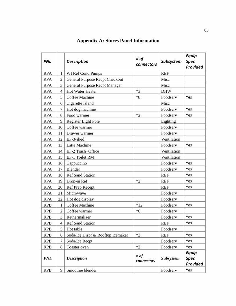
83
Appendix A: Stores Panel Information
PNL
Description # of connectors
Subsystem Equip Spec Provided
RPA 1 WI Ref Cond Pumps
REF
RPA 2 General Purpose Recpt Checkout
Misc
RPA 3 General Purpose Recpt Manager
Misc
RPA 4 Hot Water Heater *3 DHW
RPA 5 Coffee Machine *8 Foodserv Yes
RPA 6 Cigarette Island
Misc
RPA 7 Hot dog machine
Foodserv Yes
RPA 8 Food warmer *2 Foodserv Yes
RPA 9 Register Light Pole
Lighting
RPA 10 Coffee warmer
Foodserv
RPA 11 Drawer warmer
Foodserv
RPA 12 EF-3-shed
Ventilation
RPA 13 Latte Machine
Foodserv Yes
RPA 14 EF-2 Trash+Office
Ventilation
RPA 15 EF-1 Toilet RM
Ventilation
RPA 16 Cappuccino
Foodserv Yes
RPA 17 Blender
Foodserv Yes
RPA 18 Ref Sand Station
REF Yes
RPA 19 Drop-in Ref *2 REF Yes
RPA 20 Ref Prep Recept
REF Yes
RPA 21 Microwave
Foodserv
RPA 22 Hot dog display
Foodserv
RPB 1 Coffee Machine *12 Foodserv Yes
RPB 2 Coffee warmer *6 Foodserv
RPB 3 Rethermalizer
Foodserv Yes
RPB 4 Ref Sand Station
REF Yes
RPB 5 Hot table
Foodserv
RPB 6 Soda/Ice Dispr & Rooftop Icemaker *2 REF Yes
RPB 7 Soda/Ice Recpt
Foodserv Yes
RPB 8 Toaster oven *2 Foodserv Yes
PNL Description # of
connectors Subsystem
Equip Spec Provided
RPB 9 Smoothie blender
Foodserv Yes

84
RPB 10 Food service disp
Foodserv
RPB 11 Frozen Carb Bev Machine *2 Foodserv Yes
RPB 12 Carbonator
Foodserv
RPB 13 CSR/CO2 Closet Recpt
Foodserv
RPB 14 Convection oven *3 Foodserv Yes
RPB 15 Recpt shed
Misc
RPC 1 ATM
Misc
RPC 2 General purpose recept
Misc
RPC 3 Auto flush valve
Misc
RPC 4 Trash compactor
Misc
RPC 5 Roof pocket recpt/light
Misc
RPC 6 PWR wash *2 Misc
RPC 7 Display case flr recept
Misc
RPC 8 Floor recept *2 Misc
RPC 9 Walk-in ref-ash
REF
RPC 10 Serv ref DR Heat/Fan Cool
REF
RPC 11 Hill Phoenix Ref Island
REF Yes
RPC 12 Walk-in ref fan coil *2 REF
RPC 13 Soffit/coffee conv.rcpt
Misc
RPC 14 Exterior/conv recept
Misc
RPC 15 Slicer
Foodserv
RPC 16 Scale @ slicing ctr
Foodserv
RPC 17 Vestibule/conv.recept
Misc
RPC 18 Toaster oven *2 Foodserv Yes
RPC 19 Convection oven *3 Foodserv Yes
RPC 20 Irrigation sys
Misc
RPC 21 HT Trace LG & SM WI FZR
REF
RPC 22 4 door reach-in freezer-ash
REF Yes
RPD 1 Gas-simplex recpt
Gas stat
RPD 2 Veeder-root
Gas stat
RPD 3 F.E. Petro DHI Relays
Gas stat
RPD 4 Fuel Dispenser *6 Gas stat
RPD 5 Overall alarm
Misc
RPD 6 Cash register *3 Misc
PNL
Description # of
connectors Subsystem
Equip Spec Provided
RPE 1 Ceil MTD CCTV Monitor *4 Misc
RPE 2 Price changing motor
Misc
RPE 3 Fire alarm panel 'lock'
Misc
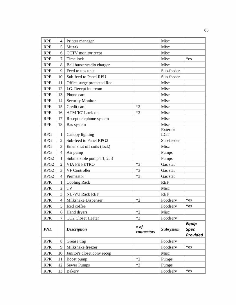
85
RPE 4 Printer manager
Misc
RPE 5 Muzak
Misc
RPE 6 CCTV monitor recpt
Misc
RPE 7 Time lock
Misc Yes
RPE 8 Bell buzzer/radio charger
Misc
RPE 9 Feed to ups unit
Sub-feeder
RPE 10 Sub-feed to Panel RPU
Sub-feeder
RPE 11 Office surge protected Rec
Misc
RPE 12 I.G. Recept intercom
Misc
RPE 13 Phone card
Misc
RPE 14 Security Monitor
Misc
RPE 15 Credit card *2 Misc
RPE 16 ATM 'IG' Lock-on *2 Misc
RPE 17 Recept telephone system
Misc
RPE 18 Bas system
Misc
RPG 1 Canopy lighting
Exterior
LGT
RPG 2 Sub-feed to Panel RPG2
Sub-feeder
RPG 3 Emer shut off coils (lock)
Misc
RPG 4 Air pump
Pumps
RPG2 1 Submersible pump T1, 2, 3
Pumps
RPG2 2 VIA FE PETRO *3 Gas stat
RPG2 3 VF Controller *3 Gas stat
RPG2 4 Permeator *3 Gas stat
RPK 1 Cooling Rack
REF
RPK 2 TV
Misc
RPK 3 NU-VU Rack REF
REF
RPK 4 Milkshake Dispenser *2 Foodserv Yes
RPK 5 Iced coffee
Foodserv Yes
RPK 6 Hand dryers *2 Misc
RPK 7 CO2 Closet Heater *2 Foodserv
PNL Description # of
connectors Subsystem
Equip Spec Provided
RPK 8 Grease trap
Foodserv
RPK 9 Milkshake freezer
Foodserv Yes
RPK 10 Janitor's closet conv recep
Misc
RPK 11 Boost pump *2 Pumps
RPK 12 Sewer Pumps *3 Pumps
RPK 13 Bakery
Foodserv Yes

86
RPK 14 Expresso *2 Foodserv
RPU 1 Quad recpt comp server *2 Misc
RPU 2 Cash register *3 Misc
RPU 3 Security monitors/VCR Mgr's
Misc
RPU 4 LOTTERY mach
Misc
RPU 5 Fee mach
Misc
RPU 6 UPS output
Sub-feeder
RPU 7 Cust Access Terminal *4 Misc
RPU 8 Checkout Extender/Monitor Mgr's *2 Misc
LPA 1 Toilet rms
Lighting
LPA 2 Deli/Backrm/Mgr
Lighting
LPA 3 Retail *2 Lighting
LPA 4 Directional Lights
Lighting
LPA 5 Checkout area
Lighting
LPA 6 Contactor coils 'lock'
Lighting
LPA 7 Night/Emer Lights 'Lock' *2 Lighting
LPA 8 Vestibule Wall Washers
Lighting
LPA 9 Exterior wall paks *3 Lighting
LPA 10 Emer Battery Packs
Lighting
LPA 11 Neon goose
Lighting
LPA 12 Lights above walk-ins
Lighting
LPA 13 Street signs *2
Exterior
LGT
LPA 14 Prep/Trash/Assoc/Elec
Lighting
LPA 15 Wall wash-retail area
Lighting
LPA 16 Checkout wall washers
Lighting
LPA 17 Front checkout
Lighting
LPA 18 Walk-in ref
Lighting
LPA 19 Retail wlk-in ref-dr light
Lighting
PNL Description # of
connectors Subsystem
Equip Spec Provided
LPA 20 FASCIA sign
Lighting
LPA 21 light shed
Lighting
LPA 22 Price sign conv. Recpt
Lighting
LPA 23 Direction signs
Lighting
LPA 24 Site lighting *4
Exterior
LGT

87
Appendix B: Outlier Identifying
Outliers are defined as data points that are statistically inconsistent with the rest of the
data. We must be careful because some “questionable” data points end up being outliers, but
others do not. Questionable data points should never be discarded without proper statistical
justification. The outliers in this research are because of meters’ problem and unread data so this
is a reasons we discard suspected outliers.
The modified Thompson tau technique is a statistical method for deciding whether to
keep or discard suspected outliers in a sample of a single variable. Here is the procedure:
The sample mean x and the sample standard deviation S are calculated in the usual
fashion. For each data point, the absolute value of the deviation is calculated as
The data point most suspected as a possible outlier is the data point with the maximum
value of δi. The value of the modified Thompson τ (Greek letter tau) is calculated from the
critical value of the student’s t PDF, and is therefore a function of the number of data points n in
the sample. τ is obtained from the expression
, where:
n is the number of data points
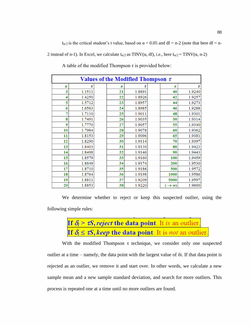
88
tα/2 is the critical student’s t value, based on α = 0.05 and df = n-2 (note that here df = n-
2 instead of n-1). In Excel, we calculate tα/2 as TINV(α, df), i.e., here tα/2 = TINV(α, n-2)
A table of the modified Thompson τ is provided below:
We determine whether to reject or keep this suspected outlier, using the
following simple rules:
With the modified Thompson τ technique, we consider only one suspected
outlier at a time – namely, the data point with the largest value of δi. If that data point is
rejected as an outlier, we remove it and start over. In other words, we calculate a new
sample mean and a new sample standard deviation, and search for more outliers. This
process is repeated one at a time until no more outliers are found.

89
Reference: Author: John M. Cimbala, Penn State University Latest revision: 12
September 2011