Moment-Based Learning of Mixture Distributions

SPUR Final Paper, Summer 2016

Kavish Gandhi and Yonah Borns-WeilMentor: Amelia Perry

Project suggested and supervised by Professor Ankur Moitra

August 4, 2016

Abstract

We study the problem of learning the parameters of a mixture of members of agiven distribution family. To do this, we apply the method of moments, dating toPearson in the late 1800’s: we directly solve for the parameters in terms of estimatedsample moments. We prove upper and lower bounds on the number of moments thatuniquely determine mixtures for various distribution families. In particular, we showthat 2k−1 moments are necessary and sufficient to determine a large class of mixturesof k one-parameter distributions, including Poissons and exponentials, and developan efficient algorithm to learn the parameters of these mixtures. Additionally, usingnatural exponential families as motivation, we ask which sets of 2k − 1 moments of afinite distribution uniquely determine its parameters, and show that this question canbe reduced to asking about the zero sets of certain Schur polynomials. We also showthat 4k−2 moments are necessary for determining a mixture of k Gaussians, matchinga known upper bound shown by Moitra and Valiant, and with this we improve theexisting lower bound on the sample complexity of learning such a mixture. We provesimilarly that 4k− 2 moments are necessary and sufficient to learn a mixture of k uni-form distributions, and conjecture that a similar result holds for general two-parameterdistributions whose moments satisfy certain polynomial dependence conditions on theparameters. Finally, for a general family of Gaussian-like distributions of the formp(x)eq(x), we derive a bound on the number of moments necessary to uniquely deter-mine a mixture that is exponential in k.

1. Introduction

Background. A rich area of modern machine learning is the learning of mixture models,with applications throughout the scientific disciplines, including biology [1], finance [2], andphysics [3, 4], among many others. The first results in the field came over 100 years agoin 1894, when biostatistician Karl Pearson studied the measurements of what he assumedwas a single crab species and discovered an as-of-yet unseen distribution. His insight wasthat he was in fact observing two species, with each having measurements following thestandard Gaussian distribution. This motivated defining a (two) Gaussian Mixture Modelas a distribution F with density function p1f1+p2f2, where p1+p2 = 1 and f1, f2 are Gaussiandensity functions. To determine the parameters of the mixture from samples (and hence thedata for each crab species), Pearson [5] invented the method of moments, in which he tookthe first five moments of a large number of samples drawn from this distribution, and solvedby hand the resulting polynomial system for the means, variances, and probabilities. Gettingfinitely many solutions, he then chose the one whose sixth moment most closely matched thesixth sample moment. His results both demonstrated the effectiveness of learning a mixturefrom its moments and the utility of learning the parameters in particular, or parameterlearning, rather than a distribution that is simply close in total variation distance, anotherrich area of study.

The problem of learning the parameters of a mixture of an arbitrary number of Gaus-sians has had a long history, where a mixture of k Gaussians is defined as the distribution

with density functionk∑i=1

pifi, where f1, . . . , fk are the component Gaussian densities and

p1, . . . , pk are mixing weights satisfyingk∑i=1

pi = 1. Many approaches to the problem since

Pearson have involved clustering, starting with Dasgupta [6] in 1999, who used clustering torigorously define a polynomial-time algorithm for separating d-dimensional Gaussians givena Ω(√d) separation between their means. The separation bound was gradually shrunk by

later authors, including Arora and Kannan [7], Dasgupta and Schulman [8] and Vempalaand Wang [9].

While these clustering results gave efficient algorithms for separated mixtures of Gaus-sians, they could not deal with even the simplest mixtures with lack of mean separationand non-negligible overlap of the components. Pearson’s moment-based approach, however,proved fruitful for these types of mixtures, and in general for arbitrary Gaussian mixtures.In 2010, Moitra, Valiant, and Kalai [10] used a robust and rigorous version of Pearson’smethod of moments to give an algorithm that learns mixtures of two Gaussians to withinparameter distance ε in time polynomial in ε, and in 2015 Hardt and Price [11] found anoptimal algorithm for the two Gaussian mixture problem with respect to sample complexity,using an approach directly based on Pearson’s polynomial. Moitra and Valiant [12], later in2010, extended their result to mixtures of k Gaussians.

Simultaneously, Belkin and Sinha [13] generalized the moment method to any mixture ofpolynomial families, or families of distributions with moments polynomial in the parameters.Their proof was non-constructive, using the Hilbert basis theorem to show that finitely

1

many moments determine such mixtures, demonstrating that the method of moments isindeed a general, powerful strategy for learning mixtures of any polynomial family. However,the bound on a sufficient number of moments was simply shown to exist, and no effectivebound was presented; the focus of this paper is on this question. Our goal is to establisheffective bounds on the number of sufficient moments for particular families of distributions,independent of the parameters of the distribution.

Our results. Our work on moment-matching begins with the simplest case of one-parameterfamilies, which are polynomial families determined by only a single parameter. The simplestone parameter distributions are the point masses, for which the corresponding mixtures arefinite distributions; in Section 2, we review the classical theory of Gaussian quadrature, whichshows that exactly 2k−1 moments are required to uniquely determine such a finite distribu-tion. Then, in Section 3, we study one-parameter distributions where the jth moment is adegree j polynomial in the parameter, and show that the problem of learning the parametersof a mixture of these distributions can be reduced to determining the finite distribution onthe same parameters, for which we know 2k − 1 moments are sufficient. From these results,in Section 4 we develop an efficient, robust algorithm for learning mixtures of one-parametersubexponential distributions with this polynomial dependence on the moment, our first mainresult, Algorithm 4.1.

In Section 5, we review the theory of exponential families and natural exponential families,which have a particularly simple form for their density functions and comprise a large classof one-parameter families. By taking the mean as the parameter, these are automaticallypolynomial families, and the condition on the degree of the moments roughly correspondsto having the variance as a function of the mean V (µ) be quadratic, which gives the naturalexponential families with quadratic variance functions (NEF-QVF’s), studied in [14] andwhich include many common distribution families. Using the method detailed in Algorithm4.1, we therefore can efficiently find the parameters of almost any NEF-QVF mixture.

This discussion motivates us to look at NEF’s with higher-degree polynomial variancefunctions, which reduces to the problem of determining finite distributions by certain lin-ear combinations of their moments. In Section 6, we consider the simplified problem ofdetermining for which a1, . . . a2k−1 the moments Ma1 , . . .Ma2k−1

determine a finite dis-tribution on k points. The main result of this section is that the moments of two distinctfinite distributions differ whenever a certain Schur polynomial in the 2k points is nonzero,which implies the following result.

Theorem 6.6, Restated. Let S = 0, a1, a2, . . . , a2k−1 where 0 < a1 < a2 < · · · < a2k−1 ∈Z, and let λ = (a2k−1−(2k−1), a2k−2−(2k−2), . . . , a1−1, 0). If sλ(z1, . . . , z2k) is nonzero forall real z1, . . . , z2k, then the moments Ma1 , . . .Ma2k−1

uniquely determine a finite distributionon k points.

Thus, we can reduce one direction of this question to finding which Schur polynomialshave only trivial zeros, and present some known partial results to that end, as well as thebroader conjecture that this occurs whenever all parts in the partition are even.

2

In Section 7, we then return to the original problem of Gaussians, and place it in context oftwo-parameter distribution families in general. We show that 4k−2 moments are sometimesnecessary to determine a mixture of k Gaussians, matching the result in [10] that it is alwayssufficient.

Proposition 7.1. There exist two mixtures of k Gaussians, F, F ′, such that F 6= F ′ andMj(F ) = Mj(F

′) for 1 ≤ j ≤ 4k − 3.

The example for necessity, however, is a special case where all means are equal, so weconjecture that in the case of distinct means, only 3k moments are necessary. Along the linesof the sufficiency proof in [12], we also show that 4k−2 moments are necessary and sufficientto uniquely determine a mixture of k uniform distributions, and conjecture that indeed 4k−2moments are sufficient to determine any mixture of a two-parameter family with momentsthat are degree at most k in each of the parameters. This conjecture is supported by somenumerical evidence in the case of Gamma and Laplace distributions.

Finally, in Section 8, we consider the problem of learning a mixture of general families ofdistributions with an arbitrary number of parameters, in the hope of getting some concreteupper bound on the number of moments required to determine these mixtures, as opposed tothe ineffective bound in [13]. We arrive at a result for a specific class of distribution familiesD of the form p(x)eq(x), when p(x) and q(x) are polynomials with degree independent of theparameters.

Proposition 8.2. Consider some F ∈ D with deg(p) = d1 − 1, deg(q) = d2 > 0. ThenO(d1d

2k2 ) moments suffice to uniquely determine a mixture of k F -distributions.

This leads us to our last conjecture, which would make explicit the ideas presented byBelkin and Sinha in [13] and give some general bound on the number of moments neededto match any mixture of members of a (not necessarily natural) exponential family, a classwhich includes nearly all named distribution families.

Conjecture 8.3. Let F be an exponential family. Then there exists a function f(k) inde-pendent of the parameters such that at most f(k) moments suffice to uniquely determine amixture of k F -distributions.

2. Finite Distributions

In this section, we summarize the classical theory of moment matching for finite (i.e. finitelysupported) distributions. In particular, we recall in Proposition 2.1 and 2.3 that 2k − 1moments are both sufficient and necessary to uniquely determine a finite distribution on kdistinct points, and outline an algorithm, whose main idea is given by Claim 2.2, that canexactly derive these points and weights given the first 2k − 1 moments. All of these resultsare well-known, although the construction in Proposition 2.3 is our own, but are stated forcompleteness.

Proposition 2.1. If F and F ′ are finite distributions on k distinct points, and Mj(F ) =Mj(F

′) for 1 ≤ j ≤ 2k − 1, then F = F ′.

3

Proof. Let F have points x1, x2, . . . , xk with weights p1, p2, . . . , pk, and F ′ have points y1, y2, . . . , ykwith weights q1, q2, . . . , qk. Suppose first that the distributions differ on at least one point;without loss of generality yk 6= xi for all i. We claim that, in this case, there exists some jsuch that 1 ≤ j ≤ 2k − 1 and Mj(F ) 6= Mj(F

′).

Define the polynomial P (x) = (x−x1) · · · (x−xk)(y− y1) · · · (y− yk−1) =2k−1∑j=0

ajxj. Note

that P (x) evaluates to 0 at all points of the finite distributions except for yk. Thus, we have

thatk∑i=1

(piP (xi)− qiP (yi)) = −qkP (yk) 6= 0. But notice that we can also write this as

k∑i=1

(piP (xi)− qiP (yi)) =2k−1∑j=1

aj

k∑i=1

(pix

ji − qiy

ji

)=

2k−1∑j=1

aj(Mj(X)−Mj(Y )).

For this to be nonzero, one of the moments must differ, as desired, so we have that if all ofthe points are not identical between distributions, the first 2k − 1 moments cannot be.

Now, consider the case in which the distributions share all of the same points; withoutloss of generality let xi = yi for all 1 ≤ i ≤ k. Letting di = pi − qi, and assuming forcontradiction that all of the moments are equal but F 6= F ′, we have that

k∑i=1

dixji = 0

for all j ≤ k − 1 (in particular, this holds for j ≤ 2k − 1, but all we need is j ≤ k − 1). Butthis implies that di = 0 for all i by multiplying each side by the inverse of the Vandermondematrix of x1, x2, . . . , xk, which exists because the xi are distinct, giving that pi = qi for all i,a contradiction of the fact that F 6= F ′. Thus, we are done.

Based on 2k−1 moments uniquely determining a finite distribution, we conceivably couldlearn a finite distribution by evaluating its first 2k− 1 moments and algorithmically solvingthe polynomial system given by these moments to derive its parameters. Note that this iscertainly not the most efficient way to learn a finite distribution, but will become useful inSection 3 when we talk about learning general one-parameter distributions.

Actually solving this polynomial system in the parameters given by the moments, whichdetermines the underlying finite distribution, is implicit in the following well-known resultfrom Gaussian quadrature, which generalizes Proposition 2.1.

Claim 2.2 (Gaussian Quadrature [15]). Given moments µj =∫ baxkdF (x) for 1 ≤ j ≤ 2k−1

of a distribution F supported on [a, b], there exist distinct (x1, . . . , xk), (w1, . . . , wk) satisfying

a ≤ xi ≤ b, 0 ≤ wi ≤ 1 for all i such thatk∑i=1

wixji = µj for all j and

k∑i=1

wi = 1.

4

In particular, these x1, . . . , xk can be derived by defining the series of orthogonal poly-nomials qi∞0 defined by the recurrence

q0(x) = (b− a)−1/2; q−1(x) = 0; βjqj(x) = (x− αj)qj−1(x)− βj−1qj−2(x),

where αj =∫ baxqj−1(x)2dF (x) and βj =

∫ baxqj(x)qj−1(x)dF (x), known constants which can

be evaluated in terms of the moments since the polynomials integrated have degree ≤ 2k−1.The x1, . . . , xk, then, are just the roots of q2k−1. From here, to find the weights, we solve forw satisfying V w = M , where

V =

1 1 · · · 1x1 x2 · · · xkx2

1 x22 · · · x2

k...

.... . .

...xk−1

1 xk−12 · · · xk−1

k ,

is the Vandermonde matrix on x1, . . . , xk, and M is the vector containing the first k < 2k−1moments, an equivalent system to our moment polynomials. Since we are given that thexi are distinct, det(V ) =

∏1≤i<j≤n

(xj − xi) is nonzero, which means that we can solve for w

simply as V −1M .

Using this, we can learn a finite distribution F on k points given 2k−1 moments as follows:first, let a = −M2(F ), b = M2(F ), so that our range of integration indeed contains all ofthe xi. Using the above recurrence, we can derive the sequence of orthogonal polynomialsto F ; our points x1, . . . , xk are then the roots of the (2k − 1)st orthogonal polynomial, andour weights can be found by evaluating V −1M . Since the first 2k − 1 moments of the finitedistribution defined with these points and weights are exactly those of the finite distributionwe are trying to learn, by Proposition 2.1, our derived finite distribution is correct.

The algorithm above allows us to precisely determine the parameters of a finite distribu-tion, given the first 2k−1 moments. We will use this as a baseline to develop a robust, generalalgorithm in Section 4 for learning mixtures of distributions belonging to one-parameter fam-ilies. In particular, the described algorithm only works when the moments are known exactly;for one-parameter families, we will develop a robust algorithm that estimates the parametersup to some error ε when the moments are known up to a specified polynomial in ε and aparameter of the distribution in question. Notice, however, that we cannot do better withexact moment-matching for finite distributions because of the following well-known result,whose proof is deferred to the appendix.

Proposition 2.3. There exist two finite distributions F, F ′, such that F 6= F ′ and Mj(F ) =Mj(F

′) for 1 ≤ j ≤ 2k − 2.

3. One Parameter Families

In this section, we use Proposition 2.1 to show that 2k − 1 moments actually uniquelydetermine a mixture of k components for a large class of one-parameter distributions, becausewe can relate their moments to those of an associated finite distribution.

5

In particular, let C be a class of one-parameter distribution families whose jth momentis a degree j polynomial in the parameter for all j ≥ 0.

Definition 3.1. Given parameters λ1, λ2, . . . , λk and mixing probabilities p1, p2, . . . , pk, a(C, k)-mixture is the distribution given by sampling from Xi with probability pi for all 1 ≤i ≤ k, where the Xi all belong to some C ∈ C.

Given a (C, k)-mixture X, we will denote by IF(x) the finite distribution specified byatoms at λ1, . . . , λk and weights p1, . . . , pk.

Proposition 3.2. Let X,X ′ be (C, k)-mixtures with components belonging to the same C ∈ C.Then Mj(X) = Mj(X

′) for 0 ≤ j ≤ 2k − 1 if and only if Mj(IF(X)) = Mj(IF(X ′)) for all1 ≤ j ≤ 2k − 1.

Proof. To prove this, we will show that, given a (C, k)-mixtures X, we can solve for momentsof X given the moments of IF(X), and vice versa. This implies the desired result.

If the components of X are X1, . . . , Xk, then Mj(X) =k∑i=1

piMj(Xi). Since Xi is a

C-distribution, Mj(Xi) =j∑

m=0

αmλmi with αj 6= 0, so we have that

Mj(X) =k∑i=1

pi

(j∑

m=0

αmλmi

)=

j∑m=0

αm

(k∑i=1

piλmi

)=

j∑m=0

αmMm(IF(X)),

so the moments of X can indeed be determined from those of IF(X).

Oppositely, we show by induction that Mj(IF(X)) can be expressed as a linear com-bination of Mi(X) for 0 ≤ i ≤ j. The base case is clearly true; now assume it is true

for all i < j that Mi(IF(X)) =i∑l=0

αlMl(X). Now, notice that, as shown previously,

Mj(X) =j∑

m=0

αmMm(IF(X)) for constants αm and αj 6= 0; moving all of the Mm(IF(X))

terms satisfying m < j to the right-hand side and expressing them as linear combinations ofMi(X) satisfying 0 ≤ i ≤ m, possible by our inductive hypothesis, we are done.

Note that, by Proposition 2.1, Mj(F ) = Mj(F′) for all 1 ≤ j ≤ 2k − 1 if and only if

F = F ′, provided the parameters are distinct, which implies that X = X ′ because, sinceF = F ′, they share the same parameters and weights. From this, we have the following:

Corollary 3.3. Given two (C, k)-mixtures X,X ′ of components with distinct parameters,X = X ′ if and only if Mj(X) = Mj(X

′) for 0 ≤ j ≤ 2k − 1.

4. A Robust Algorithm for learning (C, k)-mixtures

In this section, based on the results from Section 3, we present an robust, efficient moment-matching algorithm to learn a (C, k)-mixture. Corollary 3.3 implies that, once we learn the

6

2k − 1 moments of a (C, k)-mixture, this mixture is uniquely determined. Our first resultmakes this result robust by giving us an estimate of how well we need to learn the momentsto determine the mixture up to ±ε in the parameters.

We first show that estimating the moments of a (C, k) mixture well allows to also estimatethe moments of the corresponding finite distribution well. Note that throughout this sectionwe will assume k is held fixed, so will treat it as a constant.

Proposition 4.1. Given an estimate Mj(X), 1 ≤ j ≤ 2k − 1, of the first 2k − 1 moments

of X satisfying |Mj(X) −Mj(X)| ≤ β, Algorithm 4.1 outputs an estimate of Mj(IF(X))

satisfying |Mj(IF(X))−Mj(IF(X))| < O(β).

Proof. Following exactly the forward implication of Proposition 3.2, we can derive an esti-mate Mj(IF(X)) with the following recursive formulation:

Mj(IF(X)) =

1 if j = 0

Mj(X)−j−1∑i=0

αiMi(IF(X))

αjotherwise

.

We will prove the desired robustness statement by induction. The base case is trivial. Now,assume, for 0 ≤ i ≤ j − 1, we know all of the Mi(IF(X)) are estimates up to ciβ for some

constants ci. By assumption, we know Mj(X) up to β, so we have that, using that the αjare constants (since we are holding k fixed),

|Mj(IF(X))−Mj(IF(X)| = 1

αj

∣∣∣∣∣(Mj(X)−

j−1∑i=0

αiMi(IF(X))

)−

(Mj(X)−

j−1∑i=0

αiMi(IF(X))

)∣∣∣∣∣≤ 1

αj

(∣∣∣Mj(X)−Mj(X)∣∣∣+

j−1∑i=0

αi

(∣∣∣Mi(IF(X))−Mi(IF(X))∣∣∣))

≤ 1

αj

(β +

j−1∑i=0

αiciβ

)= O(β).

Now, similar to as defined by Moitra and Valiant [12], we will show that pairs of finitedistributions satisfying certain separation conditions must have a moment that differs by acertain amount. This will imply that their corresponding (C, k) mixtures must also have asimilar moment, as desired.

Definition 4.2. We say that a finite distribution F is ε-separated if the following twoconditions hold:

1. |xi − xj| ≥ ε for all i 6= j.

2. pi ∈ [ε, 1].

7

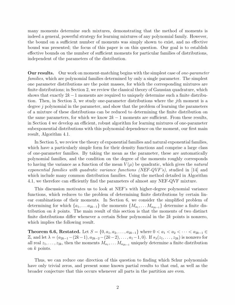
Definition 4.3. A pair of finite distributions F, F ′ is said to be (ε1, ε2)-standard if thefollowing conditions hold:

1. F and F ′ are ε1-separated.

2. |xi, x′i| ≤ 1ε1

.

3. ε2 ≤ minπ

(k∑i=1

|xi − x′π(i)|+ |pi − p′π(i)|

),

where the above minimization is taken over all permutations π : 1, 2, . . . , k → 1, 2, . . . , k.

Theorem 4.4. Given a (ε1, ε2)-standard pair of finite distributions F , F ′ with ε1 ε2, thereexists some i satisfying 1 ≤ i ≤ 2k − 1 such that

|Mi(F )−Mi(F′)| > Ω(ε4k−2

1 ε2)

The proof of this theorem is deferred to Appendix A, but the proof idea is a robustversion of that of Proposition 2.1; we construct a polynomial that goes through all but oneor two of the points of F, F ′, and show that

∫x|p(x)f(x)| is at least Ω(ε1ε

2k−12 ), which will in

turn give two moments that differ by Ω(ε1ε4k−22 ), from the upper bound on the xi.

The final step in developing an algorithm to learn mixtures of distributions in C is toshow that we can actually estimate the moments of a (C, k) mixture with a minimal numberof samples. This may not always be true, but it turns out we can estimate the momentswith probability 1− δ given O

(ε−2 log

(1δ

))samples, as proven in Proposition 4.6, when the

distribution is subexponential, defined as follows.

Definition 4.5. A distribution F is subexponential with parameter λ if the kth raw momentsatisfies Mk ≤ kkλk.

There are many equivalent definitions of subexponential distributions and the associ-ated parameter, which serve different purposes. Subexponential distributions intuitively aremeant to be those distributions with an exponential or lighter tail, and encompass many ofthe common distributions that we study.

Note that a mixture of subexponential distributions is clearly also subexponential, wherethe associated subexponential parameter is at most the maximum among its components.

Proposition 4.6. If a distribution F ∈ C is subexponential with parameter λ, then givent = O(1) there exists an algorithm taking n = O

(ε−2 log

(1δ

))samples that with probability

1− δ learns the ith moment, for i ≤ t to within ελi.

The proof of this result is deferred to Appendix A, since it is very similar to that of[11], but note that this result implies the following corollary, where we replace λ with the

standard deviation σ, since σ2 ≥k∑i=1

piσ2i from the law of total variance.

8

Corollary 4.7. Given a one-parameter distribution C ∈ C with parameter λ whose varianceσ′ is quadratic in λ and t = O(1), then there exists an algorithm taking n = O

(ε−2 log

(1δ

))samples that with probability 1− δ learns the ith moment of a mixture F of variance σ > 1of k component C-distributions for i ≤ t to within εσi.

Using all of our results, we can state a robust algorithm, Algorithm 4.1, that learns theparameters of a (C, k) mixture up to ε, given that it is subexponential.

Theorem 4.8. Let X be a (C, k), ε1-separated mixture of components X1, . . . , Xk belongingto some subexponential C ∈ C with distinct parameters satisfying λi ≤ 1

ε1for ε1 < 1. Then,

given any ε2 > 0 satisfying ε2 ε1 and a subexponential parameter γ ≥ 1 for C, Algorithm4.1 recovers the λi, wi to ±ε2 with probability 1− δ.

Proof. By Proposition 4.6, given n samples, steps 1 and 2 estimate the moments Mj(X), for1 ≤ j ≤ 2k − 1, up to

(aε−22 ε4−8k

1 γ4k−2)−0.5γj = a−0.5ε2ε4k−21 γ1−2kγj < a−0.5ε2ε

4k−21 .

By Proposition 4.1, this means that we have estimates Mj(IF(X)) of the moments of theassociated finite distribution that are also accurate up to ±bε2ε4k−2

1 , for b a constant. Choos-ing a suitably given the family C and k, Theorem 4.4 gives us that the pair of F = IF(X)

and the finite distribution F ′ on Mj(IF(X)) are not (ε1, ε2)-standard, since their moments

are too close, which gives that there exists a permutation π such that |λi − λπ(i)| < ε2 and|wi − wπ(i)| < ε2 for all 1 ≤ i ≤ k, as desired.

The remaining steps of the algorithm concern actually deriving F ′, the finite distributionon Mj(IF(X)), the correctness of which was given by Proposition 2.1 and Claim 2.2 andthe steps of which outlined in Section 2. It is worth mentioning that, because our estimatesλi are correct up to ±ε2 and |λi − λj| ≥ ε1 by assumption for i 6= j, V is still invertible.Furthermore, a and b are chosen such that |a, b| ≥M2(IF(X)), which implies that the valuesof λi lie in the integration range, as required.

9

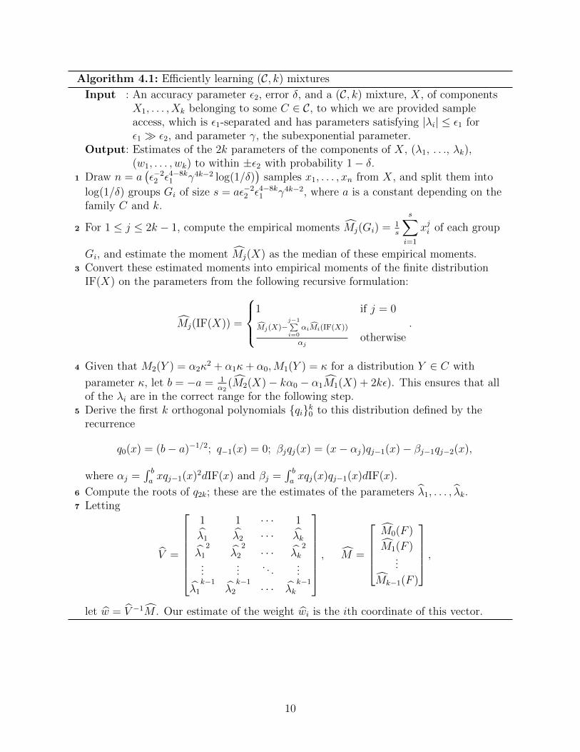
Algorithm 4.1: Efficiently learning (C, k) mixtures

Input : An accuracy parameter ε2, error δ, and a (C, k) mixture, X, of componentsX1, . . . , Xk belonging to some C ∈ C, to which we are provided sampleaccess, which is ε1-separated and has parameters satisfying |λi| ≤ ε1 forε1 ε2, and parameter γ, the subexponential parameter.

Output: Estimates of the 2k parameters of the components of X, (λ1, . . ., λk),(w1, . . . , wk) to within ±ε2 with probability 1− δ.

1 Draw n = a(ε−2

2 ε4−8k1 γ4k−2 log(1/δ)

)samples x1, . . . , xn from X, and split them into

log(1/δ) groups Gi of size s = aε−22 ε4−8k

1 γ4k−2, where a is a constant depending on thefamily C and k.

2 For 1 ≤ j ≤ 2k − 1, compute the empirical moments Mj(Gi) = 1s

s∑i=1

xji of each group

Gi, and estimate the moment Mj(X) as the median of these empirical moments.3 Convert these estimated moments into empirical moments of the finite distribution

IF(X) on the parameters from the following recursive formulation:

Mj(IF(X)) =

1 if j = 0

Mj(X)−j−1∑i=0

αiMi(IF(X))

αjotherwise

.

4 Given that M2(Y ) = α2κ2 + α1κ+ α0,M1(Y ) = κ for a distribution Y ∈ C with

parameter κ, let b = −a = 1α2

(M2(X)− kα0 − α1M1(X) + 2kε). This ensures that allof the λi are in the correct range for the following step.

5 Derive the first k orthogonal polynomials qik0 to this distribution defined by therecurrence

q0(x) = (b− a)−1/2; q−1(x) = 0; βjqj(x) = (x− αj)qj−1(x)− βj−1qj−2(x),

where αj =∫ baxqj−1(x)2dIF(x) and βj =

∫ baxqj(x)qj−1(x)dIF(x).

6 Compute the roots of q2k; these are the estimates of the parameters λ1, . . . , λk.7 Letting

V =

1 1 · · · 1

λ1 λ2 · · · λk

λ1

2λ2

2· · · λk

2

......

. . ....

λ1

k−1λ2

k−1· · · λk

k−1

, M =

M0(F )

M1(F )...

Mk−1(F )

,

let w = V −1M . Our estimate of the weight wi is the ith coordinate of this vector.

10

5. Natural Exponential Families

Our result on one-parameter families that satisfy a particular polynomial condition on theirmoments may seem unmotivated, since the condition does not obviously correspond to aparticular family of distributions. However, at least a subset of these one-parameter familiesbelong to a more general class of families of distributions parameterized by some parametervector, known as exponential families. In this section, we describe a special case of these,natural exponential families, and use this case to give examples of distribution families in C.

Definition 5.1. Consider a family of d-dimensional distributions parameterized by θ ∈ Rs,with probability density functions fXθ . We call this an exponential family if we can findfunctions h : Rd → R, η : Rs → Rs, T : Rd → Rs, A : h : Rs → R such that

fXθ(x) = h(x)eη(θ)·T (x)−A(θ).

We call η the natural parameter, T the sufficient statistic, and A the log-partition function.

This is an enormous class of parametric families of distributions, including many commondistributions such as Gaussians, Poisson distributions, and Gamma distributions, so we canrestrict a bit and still get a quite rich collection.

Definition 5.2. An exponential family is called a natural exponential family if T and η areboth the identity function.

Specifically, a natural exponential family has a density of the form

fXθ(x) = h(x)eθx−A(θ).

In this case, θ can be thought of as the parameter, though it is important to keep inmind that it may not exactly correspond to the standard definition of the parameter for thatparticular distribution.

Natural exponential families are especially motivated because they are described com-pletely by their mean or variance, as shown by the following facts, of which one can find afuller discussion in [14].

Fact 5.3. If A is the log-partition function in a natural exponential family, then the rthcumulant is given by A(r)(θ).

Notice that this gives that A′′(θ) > 0, so A′ is injective and hence invertible. From this,we can define the variance function V (µ) as a function of the mean µ = A′(θ), which impliesthe following fact.

Fact 5.4. The variance function V , together with a domain, determines the natural expo-nential family.

It is also true, for a natural exponential family, that writing the variance function allowfor a simple recurrence formula for cumulants of a member of a natural exponential family.

11

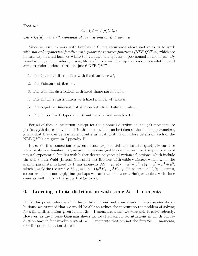
Fact 5.5.Cj+1(µ) = V (µ)C ′j(µ)

where Ck(µ) is the kth cumulant of the distribution with mean µ.

Since we wish to work with families in C, the recurrence above motivates us to workwith natural exponential families with quadratic variance functions (NEF-QVF’s), which arenatural exponential families where the variance is a quadratic polynomial in the mean. Bytransforming and considering cases, Morris [14] showed that up to division, convolution, andaffine transformations, there are just 6 NEF-QVF’s:

1. The Gaussian distribution with fixed variance σ2,

2. The Poisson distribution,

3. The Gamma distribution with fixed shape parameter α,

4. The Binomial distribution with fixed number of trials n,

5. The Negative Binomial distribution with fixed failure number r,

6. The Generalized Hyperbolic Secant distribution with fixed r.

For all of these distributions except for the binomial distribution, the jth moments areprecisely jth degree polynomials in the mean (which can be taken as the defining parameter),giving that they can be learned efficiently using Algorithm 4.1. More details on each of theNEF-QVF’s are given in Appendix B.

Based on this connection between natural exponential families with quadratic varianceand distribution families in C, we are then encouraged to consider, as a next step, mixtures ofnatural exponential families with higher-degree polynomial variance functions, which includethe well-known Wald (Inverse Gaussian) distributions with cubic variance, which, when thescaling parameter is fixed to 1, has moments M1 = µ, M2 = µ3 + µ2, M3 = µ5 + µ4 + µ3,which satisfy the recurrence Mn+1 = (2n−1)µ2Mn+µ2Mn−1. These are not (C, k)-mixtures,so our results do not apply, but perhaps we can alter the same technique to deal with thesecases as well. This is the subject of Section 6.

6. Learning a finite distribution with some 2k − 1 moments

Up to this point, when learning finite distributions and a mixture of one-parameter distri-butions, we assumed that we would be able to reduce the mixture to the problem of solvingfor a finite distribution given its first 2k− 1 moments, which we were able to solve robustly.However, as the inverse Gaussian shows us, we often encounter situations in which our re-duction may in fact involve a set of 2k − 1 moments that are not the first 2k − 1 moments,or a linear combination thereof.

12

A pertinent starting question, then, is: which sets of 2k−1 moments Ma1 ,Ma2 , . . . ,Ma2k−1

uniquely determine a finite distribution F on k points?

To approach this question, we generalize the approach outlined in the proof of Proposition2.1, in which, given a pair of unequal F, F ′, we construct a polynomial p(x) that has rootsat all but one of the points of F, F ′, thus giving a nonzero integral

∫x|p(x)(F − F ′)|. In

Proposition 2.1, we wanted this polynomial to be of degree 2k − 1, since this implied thatone of the first 2k − 1 moments differs. In this case, we want our polynomial to have atmost 2k − 1 nonzero coefficients, corresponding to xa1 , xa2 , . . . , xa2k−1 . We first show that itis possible to construct such a polynomial from the p(x) given in Proposition 2.1.

Lemma 6.1. Let S = 0, a1, a2, . . . , a2k−1 where 0 < a1 < a2 < · · · < a2k−1 ∈ Z. Givendistinct finite distributions F, F ′ on points x1, . . . , xk and y1, . . . , yk , there exists a nonzero

polynomial q(x) =∑i∈S

cixi such that q(x) is divisible by

∏ki=1(x− xi)

∏k−1i=1 (x− yi).

Proof. Let D = d1, . . . , dl = 0, 1, . . . , a2k−1 \ S. Let

U(x) =2k−1∑i=0

uixi =

k∏i=1

(x− xi)k−1∏i=1

(x− yi),

and M be the l × (l + 1) matrix such that Mij = udi−j. Because the numbers of rows ofM is l, we have that rank(M) ≤ l, which gives that nullity(M) ≥ 1. This means thatthere must exist some nonzero vector b = (b0, b1, . . . , bl) satisfying Mb = 0. Then lettingB(x) =

∑li=0 bix

i gives q(x) = B(x)U(x) to satisfy the desired properties.

It is useful to know that we can always construct such a polynomial; our goal, however,is to construct such a polynomial that has exactly 2k − 1 roots in P , since this gives us thefollowing result.

Proposition 6.2. Let S = 0, a1, a2, . . . , a2k−1 where 0 < a1 < a2 < · · · < a2k−1 ∈ Z.Given finite distributions F, F ′ on distinct points P = x1, . . . , xk, y1, . . . , yk such that F 6=F ′, there exists a nonzero polynomial q(x) =

∑i∈S

cixi such that q(x) has shares as roots all

but one of the elements of P . Then the set of moments Ma1 ,Ma2 , . . . ,Ma2k−1 uniquely

determines a finite distribution on k points.

Proof. This follows immediately from the fact that the integral∫x|q(x)(F −F ′)| is nonzero,

implying that there must exist some i ∈ S such that Mi(F ) 6= Mi(F′), since these correspond

to the nonzero coefficients of q.

One particular instance in which this polynomial is easy to construct occurs when theai are uniformly spaced with an odd difference; in other words, ai = ai−1 + j for some oddj ∈ Z+.

Proposition 6.3. Let S = a1, a2, . . . , a2k−1 = a, a + j, . . . , a + (2k − 2)j where j is anodd positive integer and a > 0. Then the set of moments Ma1 ,Ma2 , . . . ,Ma2k−1

uniquelydetermines a finite distribution on k points.

13

Proof. Let F, F ′ be two finite distributions on points x1, . . . , xk, y1, . . . , yk, where xa 6=xb, ya 6= yb for all a 6= b. First, assume that there exists some l such that yl 6= xi forall 1 ≤ i ≤ k. Without loss of generality, let k = l, and let yk be nonzero, possible because,given the above, there also exists some xj which is distinct from all of the yi for 1 ≤ i ≤ k;without loss of generality we assume that yk is nonzero, since we know that xj 6= yk. Withthis established, apply Proposition 6.2 using the polynomial

q1(X) = xaj−1∏l=0

(k∏i=1

(x− xiζ lj)k−1∏i=1

(x− yiζ lj)

)

where ζj = ei2πj , possible because the only real roots of this are 0, x1, . . . , xk, y1, . . . , yk−1.

If there exists no such l, then without loss of generality let xi = yi for all i. BecauseF 6= F ′, there must exist some j such that pj 6= qj; without loss of generality, let j = k.Then, similarly define the polynomial

q2(X) = xaj−1∏l=0

(k−1∏i=1

(x− xiζ lj)k−1∏i=1

(x− yiζ lj)

)

and apply Proposition 6.2, noting that the integral∫x|q2(x)(F −F ′)| is still nonzero because

of the difference in weights.

When the ai are uniformly spaced with an even difference, then it is easy to constructcounterexamples in which two different mixtures share the same set of moments, since eitherthe moments are all even or all odd. In particular, if all of the moments are even, then givena mixture F with component parameters xi, pi, the mixture F ′ with parameters −xi, piclearly has the same moments. Oppositely, if all of the moments are even, then, given amixture F with component parameters (x1,−x1, x2, . . . , xk−1), (p1, p1, p2, . . . , pk−1), then themixture F ′ with component parameters (y1,−y1, x2, . . . , xk−1), (p1, p1, p2, . . . , pk−1) has thesame moments but is a distinct mixture if we pick y1 6= x1.

In general, we can also approach this problem as follows: from Proposition 6.1, we knowthat it is always possible to extend a polynomial g(x) with roots at all but one of thepoints of the two mixtures to another polynomial g?(x) with nonzero coefficients only atthe known moments. If the same cannot be done for h(x) =

∏ki=1(x − xi)(x − yi), which

has all of the points as roots, then g?(x) cannot be divisible by h(x), which means that∫x|g?(x)(F −F ′)| must be nonzero, as desired. Thus, one approach is to determine for which

sets a1, a2, . . . , a2k−1 we can show that h(x) cannot be extended.

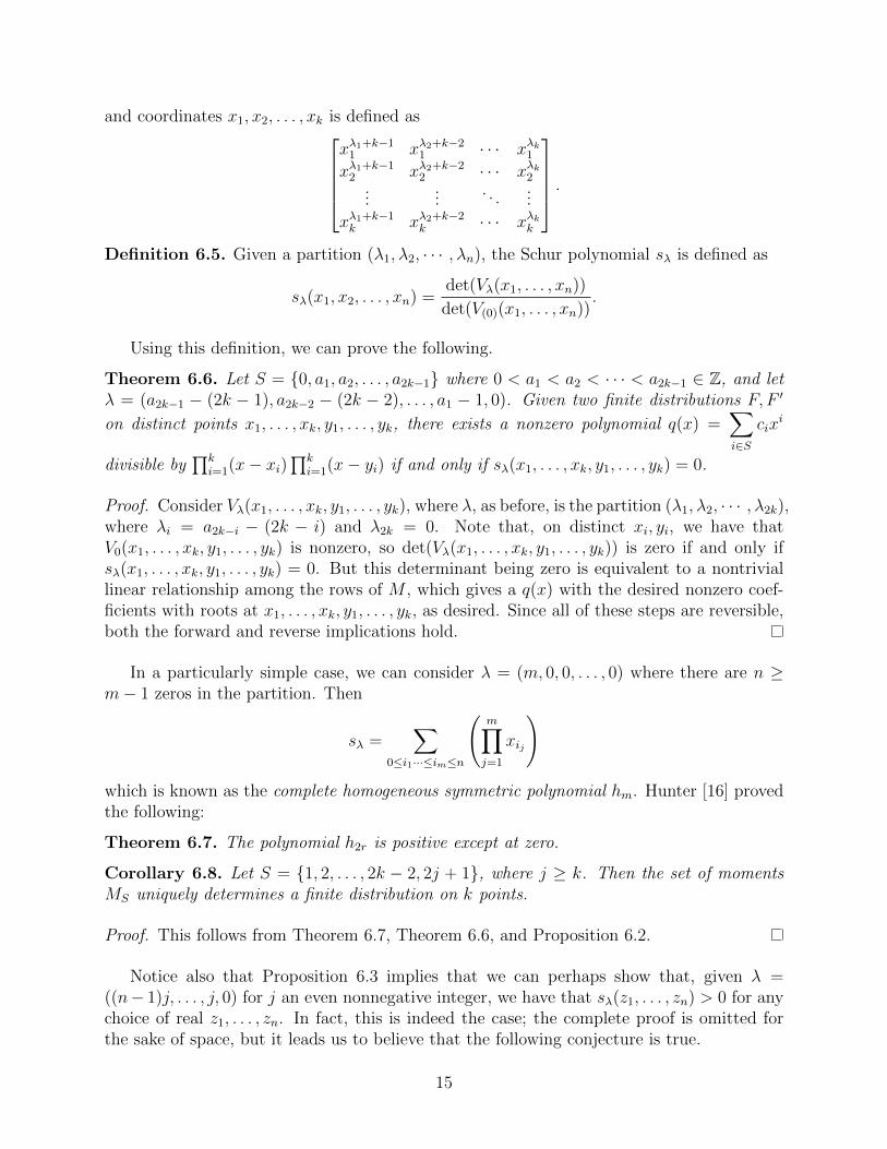
It turns out that a sufficient condition involves the Schur polynomials sλ(x1, x2, . . . , xk, y1, . . . , yk),where λ is the partition (λ1, λ2, · · · , λ2k−1, 0), λi = a2k−i− (2k− i). These polynomials havea number of equivalent definitions; we will present the one most useful for our discussion.

Definition 6.4. A generalized Vandermonde matrix Vλ(x1, . . . , xk) on λ = (λ1, λ2, · · · , λk)

14

and coordinates x1, x2, . . . , xk is defined asxλ1+k−1

1 xλ2+k−21 · · · xλk1

xλ1+k−12 xλ2+k−2

2 · · · xλk2...

.... . .

...

xλ1+k−1k xλ2+k−2

k · · · xλkk

.Definition 6.5. Given a partition (λ1, λ2, · · · , λn), the Schur polynomial sλ is defined as

sλ(x1, x2, . . . , xn) =det(Vλ(x1, . . . , xn))

det(V(0)(x1, . . . , xn)).

Using this definition, we can prove the following.

Theorem 6.6. Let S = 0, a1, a2, . . . , a2k−1 where 0 < a1 < a2 < · · · < a2k−1 ∈ Z, and letλ = (a2k−1 − (2k − 1), a2k−2 − (2k − 2), . . . , a1 − 1, 0). Given two finite distributions F, F ′

on distinct points x1, . . . , xk, y1, . . . , yk, there exists a nonzero polynomial q(x) =∑i∈S

cixi

divisible by∏k

i=1(x− xi)∏k

i=1(x− yi) if and only if sλ(x1, . . . , xk, y1, . . . , yk) = 0.

Proof. Consider Vλ(x1, . . . , xk, y1, . . . , yk), where λ, as before, is the partition (λ1, λ2, · · · , λ2k),where λi = a2k−i − (2k − i) and λ2k = 0. Note that, on distinct xi, yi, we have thatV0(x1, . . . , xk, y1, . . . , yk) is nonzero, so det(Vλ(x1, . . . , xk, y1, . . . , yk)) is zero if and only ifsλ(x1, . . . , xk, y1, . . . , yk) = 0. But this determinant being zero is equivalent to a nontriviallinear relationship among the rows of M , which gives a q(x) with the desired nonzero coef-ficients with roots at x1, . . . , xk, y1, . . . , yk, as desired. Since all of these steps are reversible,both the forward and reverse implications hold.

In a particularly simple case, we can consider λ = (m, 0, 0, . . . , 0) where there are n ≥m− 1 zeros in the partition. Then

sλ =∑

0≤i1···≤im≤n

(m∏j=1

xij

)which is known as the complete homogeneous symmetric polynomial hm. Hunter [16] provedthe following:

Theorem 6.7. The polynomial h2r is positive except at zero.

Corollary 6.8. Let S = 1, 2, . . . , 2k − 2, 2j + 1, where j ≥ k. Then the set of momentsMS uniquely determines a finite distribution on k points.

Proof. This follows from Theorem 6.7, Theorem 6.6, and Proposition 6.2.

Notice also that Proposition 6.3 implies that we can perhaps show that, given λ =((n− 1)j, . . . , j, 0) for j an even nonnegative integer, we have that sλ(z1, . . . , zn) > 0 for anychoice of real z1, . . . , zn. In fact, this is indeed the case; the complete proof is omitted forthe sake of space, but it leads us to believe that the following conjecture is true.

15

Conjecture 6.9. If λ is a partition with only even parts and last part 0, then sλ(x1, . . . , xk, y1, . . . , yk)is positive away from zero.

7. Two-Parameter Mixtures

Our results to this point have concerned only one-parameter distributions; in this section,we consider how these techniques extend two-parameter distributions. In particular, Moitraand Valiant [12] previously showed that 4k − 2 moments suffice to uniquely determine amixture of k Gaussians; we show that this is a necessary condition.

Proposition 7.1. There exist two mixtures of k Gaussians, F, F ′, such that F 6= F ′ andMj(F ) = Mj(F

′) for 1 ≤ j ≤ 4k − 3.

Proof. Let the means of F and F ′, respectively, be denoted µ1, µ2, . . . , µk andm1,m2, . . . ,mk,and the variances be denoted σ2

1, . . . , σ2k and ν2

1 , . . . , ν2k . Let µ1 = µ2 = · · · = µk = m1 =

m2 = · · · = mk = 0, which causes the odd moments of F and F ′ to all be 0, and the

even moments M2j(F ),M2j(F′) to be

k∑i=1

piσ2ji ,

k∑i=1

piν2ji ; in particular, they represent the

moments of finite distributions at points σ2i , ν

2i . From Proposition 2.3, then, given σ2

i , we canchoose ν2

i (we can ensure positivity by taking our interval to be [0, 1], which by Proposition2.2 implies that our ν2

i fall in that range) to match the first 2k − 2 moments of these finitedistributions, which we implies that we match up to the (4k − 4)th even moment of F, F ′.Since the (4k − 3)rd moment and indeed all of the odd moments are matched by the factthat they all are zero, we have the desired result.

Note that the above construction can actually match 4k− 3 moments for any mixture ofk Gaussians in which the means are all equal. We can see this by the fact that the abovemixtures having equal moments implies they have equal cumulants, and we can shift thefirst cumulant, the mean, without changing the later cumulants, implying the desired result.

However, this matching of many moments seems to be specific to the case in which manyof the means are equal; we suspect that as the means are separated, the number of momentsthat suffice to determine the distribution becomes smaller:

Conjecture 7.2. Given a mixture of k Gaussians F such that µi 6= µj for all i 6= j, then3k moments suffice to uniquely determine F .

Other two-parameter distributions also satisfy that 4k − 2 moments are both necessaryand sufficient to uniquely determine a k-distribution mixture.

Proposition 7.3. If F and F ′ are two mixtures of k uniform distributions1, then F = F ′ ifand only if Mj(F ) = Mj(F

′) for 1 ≤ j ≤ 4k − 2.

1We define a uniform mixture as a mixture of k uniform distributions on [ai, bi], with bi ≤ ai+1 for all i.This is to ensure that it is even possible to distinguish mixtures from their density functions.

16

The proof of this result is deferred to the appendix; it is very similar to that of Proposition2.1 in establishing an upper bound by finding a polynomial matching the sign of f(x) = F−F ′of degree at most 4k − 2, and establishing a lower bound by finding particular settings forthe parameters that make all odd moments 0, as in the Gaussian case.

We suspect the above upper bounds for Gaussians and uniform distributions are similarlytrue for Laplace and Gamma distributions; we found numerical evidence with Mathematicathat 6 moments suffice to determine a mixture of two components for each of these distribu-tions, for example. We conjecture that this is sufficient in the general case of two parameterdistributions whose moments are degree k in each of the parameters.

Conjecture 7.4. Let C be a two-parameter distribution whose moments are degree at mostk in each of the parameters. If X and X ′ are two mixtures of k C-distributions, then X = X ′

if Mj(X) = Mj(X′) for 1 ≤ j ≤ 4k − 2.

8. General Mixtures

All of the results up to this point have shown that the number of moments required to learnone or two parameter distributions, given some polynomial condition on their moments interms of the parameters, is some (linear) function of k independent of the parameters. Thefollowing result extends this to a general family of distributions with an arbitrary numberof parameters and gives a bound on the number of sufficient moments exponential in k.

Definition 8.1. Let D denote the class of distribution families of the form h(θ)p(x)eq(x)η(θ),where p(x) and q(x) are polynomials whose degrees are independent of θ.

Proposition 8.2. Consider some F ∈ D with deg(p) = d1 − 1, deg(q) = d2 > 0. ThenO(d1d

2k2 ) moments suffice to uniquely determine a mixture of k F -distributions.

Proof. Let G be a mixture of k F -distributions with parameters θ1, . . . , θk, and G′ an-other mixture of k F -distributions with parameters θ′1, . . . , θ

′k. Let 2k = j, and define

g(x) = G − G′ =j∑i=1

pi(x)eqi(x), where we incorporate the parameters as constants in the

polynomials, since they are fixed for each component. We first prove that g(x) has atmost O(d1d

j2) by induction on j; it is clear in the base case j = 0. Now, assume it is

true for j − 1, and rewrite g(x) = p2k(x)eq2k(x) +2k−1∑i=1

pi(x)eqi(x). This is 0 if and only if

g2(x) = p2k(x) +2k−1∑i=1

pi(x)eqi(x)−qk(x) is 0, by quotienting out eq2k(x). Taking d1 derivatives of

g2(x) and using the fact that the number of zeroes of a function is at most one more thanthe number of zeroes of its derivative, we get that g(x) has at most d1 more zeroes than

g3(x) =2k−1∑i=1

p′i(x)eqi(x)−qk(x), where p′i(x) = ( ddx

(qi(x)− qk(x)))d1 · pi(x), which has degree at

most d1(d2 − 1) + d1 = d1d2. By our inductive step, g3(x) has at most O(d1d2(d2k−12 )) =

O(d1d2k2 ) zeroes, which means that g(x) has at most d1 +O(d1d

2k2 ) = O(d1d

2k2 ) zeroes.

17

Letting the number of zeroes of g(x) be a, we can construct a polynomial h(x) of de-gree a that matches the sign of g(x), which implies, following our usual argument, that∫x|h(x)g(x)|dx > 0 so one of the first a = O(d1d

2k2 ) moments of G and G′ differ.

This argument only works when d1, d2 are constants independent of the parameters, inwhich case it gives us an effective upper bound on a sufficient number of moments basedsolely on the number of components of the mixture. Examples of well-known families thatsatisfy this property include Gaussians, Maxwell–Boltzmann distributions, and Rayleighdistributions. However, our bound is still not linear or even polynomial in k, unlike allbounds in previous sections; this is not especially surprising, since the techniques used inProposition 8.2 do not use much about the structure of the distribution, and we suspect thatthis bound can be improved in many cases.

We conjecture that an effective bound in terms of k should always exist, independentof the parameters, in cases in which the distribution family is an exponential family. Wesuspect that, for natural exponential families at least, this bound is linear in k.

Conjecture 8.3. Let F be an exponential family. Then there exists a function f(k) inde-pendent of the parameters such that at most f(k) moments suffice to uniquely determine amixture of k F -distributions.

9. Future Work

Looking to the future, in the one-parameter domain, completely classifying the zero setsof Schur polynomials is still open, which would help in determining which sets of 2k − 1moments uniquely determine a mixture. Another question of interest is the number orproperties of additional moments necessary in cases in which a set of 2k−1 moments do notuniquely determine a finite distribution. The hope is to be able to eventually generalize thissufficiency condition involving Schur polynomials to linear combinations of moments, as thiswould then allow for the implementation of a moment-matching algorithm for mixtures ofone-parameter distributions not in C, such as natural exponential families with higher-degreepolynomial variance functions.

Furthermore, there is much work to be done with two-parameter families and exponentialfamilies in general. It is still open, in the generic case with means separated, whether only3k moments suffice to uniquely determine a Gaussian, or whether 4k − 2 moments are stillneeded; we conjectured that the former is true. Another possible area of work is generalizingour upper and lower bound techniques to get an effective bound polynomial or linear in k forgeneral two-parameter mixtures, and in fact any effective bound in terms of k in this caseand in the general case of exponential families is still open.

Finally, outside of a single specific result for Gaussians in [11], almost no work has beendone on establishing sample complexity lower bounds for learning mixtures of a certaindistribution family. We expect that such arguments would follow [11] and use distancemetrics to turn a condition on the number of moments necessary to uniquely determine a

18

distribution into a statistical lower bound, but for which families such an argument holds isstill a largely unexplored question.

10. Acknowledgments

We would like to thank Amelia Perry for being a wonderful mentor, as well as providingextensive suggestions for and review of this paper. We would also like to thank ProfessorAnkur Moitra and Professor David Jerison for helpful discussions about the project, as wellas Slava Gerovitch and SPUR as a whole for giving us such a rewarding research experience!

References

[1] P. Boettcher, P. Moroni, G. Pisoni, and D. Gianola, “Application of a finite mixturemodel to somatic cell scores of Italian goats,” Journal of dairy science, vol. 88, no. 6,pp. 2209–2216, 2005.

[2] I. D. Dinov, “Expectation maximization and mixture modeling tutorial,” Statistics On-line Computational Resource, 2008.

[3] R. Fruhwirth and M. Liendl, “Mixture models of multiple scattering: computation andsimulation,” Computer physics communications, vol. 141, no. 2, pp. 230–246, 2001.

[4] K. Tanaka and K. Tsuda, “A quantum-statistical-mechanical extension of Gaussianmixture model,” in Journal of Physics: Conference Series, vol. 95, p. 012023, IOPPublishing, 2008.

[5] K. Pearson, “Contributions to the mathematical theory of evolution,” PhilosophicalTransactions of the Royal Society of London. A, vol. 185, pp. 71–110, 1894.

[6] S. Dasgupta, “Learning mixtures of Gaussians,” in Foundations of Computer Science,1999. 40th Annual Symposium on, pp. 634–644, IEEE, 1999.

[7] S. Arora, R. Kannan, et al., “Learning mixtures of separated nonspherical Gaussians,”The Annals of Applied Probability, vol. 15, no. 1A, pp. 69–92, 2005.

[8] S. Dasgupta and L. J. Schulman, “A two-round variant of EM for Gaussian mixtures,” inProceedings of the Sixteenth conference on Uncertainty in artificial intelligence, pp. 152–159, Morgan Kaufmann Publishers Inc., 2000.

[9] S. Vempala and G. Wang, “A spectral algorithm for learning mixture models,” Journalof Computer and System Sciences, vol. 68, no. 4, pp. 841–860, 2004.

[10] A. T. Kalai, A. Moitra, and G. Valiant, “Efficiently learning mixtures of two Gaussians,”in Proceedings of the forty-second ACM symposium on Theory of computing, pp. 553–562, ACM, 2010.

19

[11] M. Hardt and E. Price, “Sharp bounds for learning a mixture of two gaussians,”arXiv:1404.4997, 2014.

[12] A. Moitra and G. Valiant, “Settling the polynomial learnability of mixtures of Gaus-sians,” in Foundations of Computer Science (FOCS), 2010 51st Annual IEEE Sympo-sium., pp. 93–102, IEEE, 2010.

[13] M. Belkin and K. Sinha, “Polynomial learning of distribution families,” in Foundationsof Computer Science (FOCS), 2010 51st Annual IEEE Symposium on, pp. 103–112,IEEE, 2010.

[14] C. N. Morris, “Natural exponential families with quadratic variance functions,” TheAnnals of Statistics, pp. 65–80, 1982.

[15] C. F. Gauss, “Methodus nova integralium valores per approximationem inveniendi,”Commentationes Societatis regiae scientarium Gottingensis recentiores, vol. 3, pp. 39–76, 1814.

[16] D. Hunter, “The positive-definiteness of the complete symmetric functions of evenorder,” in Mathematical Proceedings of the Cambridge Philosophical Society, vol. 82,pp. 255–258, Cambridge Univ Press, 1977.

20

A. Proofs of Results

We prove here those results from the body of the paper whose proofs were deferred to theappendix for the sake of space.

Proof of Proposition 2.3. Let µ be the uniform distribution on [0, 1], and let p0, p1, p2, . . . bethe sequence of orthogonal polynomials to this distribution. Let f = p2k−1, and notice thatf is orthogonal to any polynomial of degree ≤ 2k − 2, since such a polynomial can alwaysbe written as a linear combination in p0, p1, . . . , p2k−2. Now, consider the distribution µ′ on[0, 1] with density g(x) = 1 + εf(x), where ε is sufficiently small that g(x) > 0 on [0, 1].Notice that this is indeed a valid distribution because∫ 1

0

dµ′ =

∫ 1

0

dµ+ ε

∫ 1

0

f(x)x0dµ = 1,

by orthogonality of f . Similarly, by orthogonality, we get that, for j ≤ 2k − 2, the jthmoment of µ′ is

Ey∼µ′ [yj] =

∫ 1

0

yjdµ′ =

∫ 1

0

yjdµ+ ε

∫ 1

−1

yjf(x)dµ =

∫ 1

0

yjdµ = Ey∼µ[yj],

as desired. When j = 2k − 1, f(x) is no longer orthogonal to yj, which gives that

ε∫ 1

0yjf(x)dµ(x) 6= 0 so Ey∼µ′ [yj] 6= Ey∼µ[yj]. Thus, µ and µ′ are two probability distribu-

tions which match on their first 2k − 2 moments but have different (2k − 1)st moments.

From here, we apply Proposition 2.2 to generate F = I(µ), and F ′ = I(µ′), the uniquefinite distributions that match µ and µ′ on their first 2k−1 moments. Since this implies thatF and F are finite distributions that match on their first 2k− 2 moments but have different(2k − 1)st moments, we are done.

Proof of Theorem 4.4. Let F have points x1, x2, . . . , xk with weights p1, p2, . . . , pk, F′ have

points y1, y2, . . . , yk with weights q1, q2, . . . , qk, and let f(x) = F − F ′ be the difference inprobability densities. We will split our argument into two cases: separation in the points ofthe mixture and separation in the weights.

Case 1: Separation in Points

We suppose in this case that there is separation in the points of the mixture; in other words,that there exists some point a ∈ x1, . . . , xk, y1, . . . , yk such that |a−xi| & ε2 for all xi 6= a,|a − yi| & ε2 for all yi 6= a. Without loss of generality let this point be yk, and consider, asin Proposition 2.1, the polynomial

P1(x) =

(k∏i=1

(x− xi)

)(k−1∏i=1

(x− yi)

)=

2k−1∑j=0

ajxj.

We know that this is zero everywhere except for yk, and also that qk & ε1. Furthermore,by ε1-separation, there can be at most one point xi such that yk − xi = Θ(ε2); for all other

21

points z ∈ x1, . . . , xk, y1, . . . , yk/xi, yk, |yk − z| & ε1. This gives us that∣∣∣∣∫x

f(x)P1(x)dx

∣∣∣∣ = |qkP1(yk)| & ε2k−11 ε2,

as desired.

Case 2: Separation in Weights

In the second case, we do not have separation in the points, so each point xi must have aunique point yj such that |xi − yj| = o(ε2); there cannot exist more than one such point foreach xi by the ε1 separation between the points within mixtures. Without loss of generalitylet |xi − yi| = o(ε2) for all i. Now, we know, because F, F ′ are (ε1, ε2) standard, thatthere must be separation in the weights; in other words, there must exist some l such that|pl − ql| = Θ(ε2); without loss of generality let l = k, and let a = |xk − yk|.

If we picked a polynomial having one of these points as a root, the value of the polynomialat the other would be too small to give our desired moment estimation. With this in mind,consider the point b = xi+ c · (sgn(yi−xi)ε2) where c is chosen such that |b−yi|, |b−xi| & ε1for all i 6= k, and |b − yk|, |b − xk| & ε2, possible by the ε1-separation of F, F ′ and the o(ε2)closeness of yk and xk. With this established, define the polynomial

P2(x) =

(k−1∏i=1

(x− xi)

)(k−1∏i=1

(x− yi)

)(x− b) =

2k−1∑j=0

bjxj.

Notice that P2(x) is zero everywhere except for xk and yk. We want to evaluate pkP (xk)−qkP (yk), since the absolute value of this is exactly the integral |

∫xP2(x)f(x)dx|. Without

loss of generality let pk > qk; in particular, we know that pk − qk & ε2. From this, noticethat |pk

qk| ≥ 1 + ε2. We now want to show that P (yk)

P (xk) 1 + ε2, which will also us to bound

|∫xP2(x)f(x)dx|. Notice that each term of P2(xk) and P2(yk), excepting (x− b), are Ω(ε1),

and in particular differ by a. Thus, the multiplicative factor by which these terms differis at most ε1+a

ε1, so in total, excluding the x − b term, the multiplicative factor is at most

(1 + aε1

)k 1 + ka, since ε1 a. Finally, notice that because b is chosen to be farther fromxi, (xi − b) is larger than (yi − b), the maximum multiplicative factor that this contributes

to P (yk)P (xk)

is 1. Thus, we have that P (yk) & (1 + ka)P (xk), so

pkP (xk)− qkP (yk) & qkP (xk)((1 + ε2)− (1 + ka)) & ε2qkP (xk).

Since P (xk) & ε2k−21 ε2 and qk & ε1, this gives that∣∣∣∣∫

x

f(x)P2(x)dx

∣∣∣∣ & ε2ε2k−11 ,

as in the first case.

Using Case 1 and Case 2 to find differing moments

From our two cases, we have that, regardless of the closeness of the points, we have thatthere exists a polynomial Pi(x) such that |

∫xP2(x)f(x)dx| & ε2k−1

1 ε2. Now, notice that each

22

coefficient aj and bj of Pi(x) are O(ε−2k+11 ), since each polynomial is of degree 2k − 1 and

the xi, yi are bounded above by 1ε1

. Thus, we have that∣∣∣∣∫x

P2(x)f(x)dx

∣∣∣∣ . ε−2k+11

∣∣∣∣∫x

xif(x)dx

∣∣∣∣ ,which gives, by our previous bounds, that∣∣∣∣∫

x

xif(x)dx

∣∣∣∣ =

∣∣∣∣∣k∑i=1

Mi(F )−Mi(F′)

∣∣∣∣∣ & ε4k−21 ε2.

This implies that there must exist some i such that |Mi(F ) − Mi(F′)| > Ω(ε4k−2

1 ε2), asdesired.

Proof of Proposition 4.6. The proof of this is almost identical to that of Lemma 3.2 in [11].Let s = 2

ε2(2t)2t−1 = O( 1ε2

), and partition the samples xi into groups of size s. Consider

taking the empirical moment of each group. Because F is sub-exponential, Mp(F ) ≤ ppλp

by definition, so we have that

Var(xpi ) ≤ E(x2pi ) ≤ (2p)2pλ2p

Now, consider the empirical pth moment of a group Mp = 1s

s∑i=1

xpi ; the above bound gives

that Var(Mp

)≤ (2p)2pλ2p

s.

By Chebyshev’s inequality, we then have that

P(∣∣∣Mp −Mp

∣∣∣ > λp(2p)p√cs

)≤ c.

Letting c = 14t

and plugging in for s gives

P(∣∣∣Mp −Mp

∣∣∣ > ελp)≤ 1

4t

By a union bound in each group this gives

P(∣∣∣Mp −Mp

∣∣∣ ≤ ελp)≥ 3

4

for all p ≤ t. From this, because there are O(log(1/δ)) groups, the probability that more

than half of the groups satisfy P(∣∣∣Mp −Mp

∣∣∣ ≤ ελp)

is at most 1 − δ, which means that,

if we take the median of our estimated moments for each of the groups, it will satisfy thedesired bound, and we are done.

23

Proof of Proposition 7.3. We first prove that 4k − 2 moments is an upper bound, the ifdirection of this proof. To do this, assume F 6= F ′, and let f(x) = F − F ′ be the differencein probability densities. We will show that there exists a polynomial p(x) of degree at most4k − 2 such that

∫x|p(x)f(x)| > 0. To do this, consider the zeroes of f(x); these can only

occur when the value of f(x) changes, which occurs only at the left or right edge of one ofthe uniform distributions in one of the mixtures. There are 2k such distributions, so thereare 4k changes in value in total. However, two of these, the right and leftmost, do not entaila sign change, since past each of these f(x) = 0 for all x. Let these two boundary points bea and b, respectively, and, With this in mind, let the set of zeroes of f(x) between a and b be

r1, r2, . . . , rj, where j ≤ 4k−2. Then, defining p(x) = c(x−r1)(x−r2) · · · (x−rj) =4k−2∑i=0

αixi,

we can pick c ∈ −1, 1 such that p(x) matches the sign of f(x) at all x. Since we cannot havef(x) = 0 for all x because F 6= F ′, we then have that

∫x|p(x)f(x)| > 0, as desired. This is

equivalent to saying that4k−2∑i=1

αi

∫x

|xif(x)| > 0, which implies that∫x|xjf(x)| 6= 0 for some

j, or that Mj(F ) 6= Mj(F′). Thus, if F 6= F ′, some pair of the first 4k − 2 moments differs,

so 4k − 2 moments are indeed sufficient to determine a mixture of k uniform distributions.

The only if direction proceeds similarly as in the Gaussian case. Let the uniform distri-butions of F have parameters (a1, b1), (a2, b2), . . . , (ak, bk) and those of F ′ have parameters(c1, d1), (c2, d2), . . . , (ck, dk). Now, let ai = −bi and ci = −di. Using that the moments of auniform distribution with parameters (a, b) are Mn = bn+1−an+1

(n+1)(b−a), this makes all odd moments

of the uniform distributions in F, F ′ to be 0, which means that all odd moments of F, F ′

are zero, since they are just convex combinations of their components. The even moments,

in turn, are b2ni and d2n

i , so the even moments of F are M2n(F ) =k∑i=1

pib2ni , and similarly

for F ′. This gives that M2n(F ) is equal to the nth moment of a finite distribution withpoints at b2

i and weights pi; by Proposition 2.3 we can match the first 2k−2 moments of thisdistribution by picking corresponding positive d2

i (as in the Gaussian case, we can ensurepositivity by taking our interval to be [0, 1], which by Proposition 2.2 implies that our d2

i

fall in that range), implying that the even moments of F, F ′ match up to 4k − 4; since weknow from our choice of ai that the odd moments match since they are all 0, we have a pairof F, F ′ such that the first 4k − 3 moments match, implying our lower bound.

24

B. Natural Exponential Families with Quadratic Variance Functions

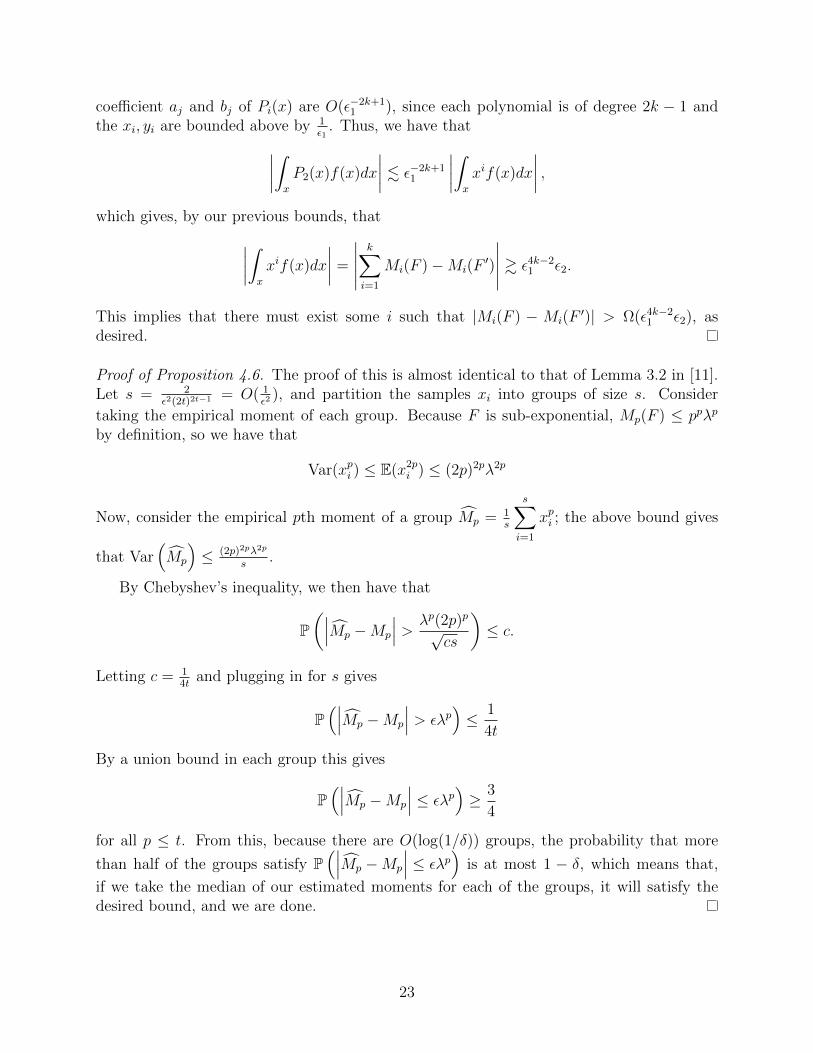
In Table 1 below, we give the probability density function, variance function, cumulants, and moment recurrence for (up toaffine transformations, division, and convolution) five of the NEF-QVF’s, omitting the generalized hyperbolic secant distributiondue to its complicated and esoteric nature. Excluding the binomial distribution, these are examples of well-known distributionwhose mixtures that can be learned efficiently by Algorithm 4.1.

Distribution PDF Variance FunctionCumulants or

Cumulant RecurrenceMoments or

Moment RecurrenceGaussian withfixed variance

f(x) = 1√2πσ2

e−(x−µ)2

2σ2 V (µ) = σ2 C1 = µ, C2 = σ2,Ck = 0 ∀k ≥ 3

Mk = µMk−1 + (k − 1)σ2Mk−2

Poisson distribution P (x) = λk

k!e−λ V (µ) = µ Ck = µ ∀k ≥ 1 Mk = µMk−1 + µd(Mk−1)

dµ

Gamma Distributionwith Fixed Shape

f(x) = xr−1

βrΓ(r)e−

xβ V (µ) = µ2

rCk = (k−1)!

rµk Mk =

∏k−1j=0(r + j)

(µr

)kBinomial Distributionwith Fixed # of Trials

P (x) =(nx

)px(1− p)n−x V (µ) = − 1

nµ2 + µ Ck =

(−µ2

n+ µ)C ′k(µ)

Mk = µMk−1+µ(n−µ)

nM ′

k−1(µ)Negative Binomial

Distribution with FixedFailure Number

P (x) = Γ(x+r)Γ(r)x!

px(1− p)r V (µ) = 1rµ2 + µ Ck(µ) =

(1rµ2 + µ

)C ′k−1(µ)

Mk(µ) = µMk−1+µ(µr

+ 1)M ′

k(µ)

Table 1: The probability distribution functions, variance functions, cumulants, and moments of five of the six NEF-QVF’s.

25