1

MOLECULAR SIMULATION OF PHASE EQUILIBRIA FOR WATER -

METHANE AND WATER - ETHANE MIXTURES

Jeffrey R. Errington1,2, Georgios C. Boulougouris3,4, Ioannis G. Economou3,* ,

Athanassios Z. Panagiotopoulos1,2 and Doros N. Theodorou3,5

1School of Chemical Engineering, Cornell University, Ithaca, NY 14853

2Institute for Physical Science and Technology and

Department of Chemical Engineering, University of Maryland,

College Park, MD 20742

3Molecular Modelling of Materials Laboratory, Institute of Physical Chemistry,

National Research Centre for Physical Sciences “Demokritos”,

GR-15310 Aghia Paraskevi Attikis, Greece

4Department of Chemical Engineering, National Technical University of Athens,

GR-15773 Zografos, Athens, Greece

5Department of Chemical Engineering, University of Patras, GR-26500 Patras, Greece

Submitted to the Journal of Physical Chemistry B,

March 11, 1998

* Author to whom all correspondence should be addressed at economou@cyclades.nrcps.ariadne-t.gr. Fax: ++ 30 1 651 1766

2

Abstract

Monte Carlo simulations were used to calculate water - methane and water - ethane phase

equilibria over a wide range of temperatures and pressures. Simulations were performed from

room temperature up to near the critical temperature of water and from sub-atmospheric pressure

to 3000 bar. The Henry’s law constants of the hydrocarbons in water were calculated from

Widom test particle insertions. The Gibbs ensemble Monte Carlo method was used for

simulation of the water-rich and hydrocarbon-rich phases at higher pressures. Two recently

proposed pair-wise additive intermolecular potentials that describe accurately the pure component

phase equilibria were used in the calculations. Equations of state for associating fluids were also

used to predict the phase behavior. In all cases, calculations were compared to experimental data.

For the highly non-ideal hydrogen bonding mixtures studied here, molecular simulation-based

predictions of the mutual solubilities are accurate within a factor of two, which is comparable to

the accuracy of the best equations of state.

3

Introduction

The accurate knowledge of water - hydrocarbon phase equilibria and mutual solubility is

important for equipment design and operation of various processes in the petroleum refining and

petrochemical industry, natural and petroleum gas production, and environmental control. For

many such applications, the temperature and the pressure of the system vary substantially. A

number of experimental studies are available in the literature,1-4 but more data are needed, and

their measurement is quite difficult and expensive. Therefore, it is highly desirable to develop

predictive approaches for determining the thermodynamics of water - hydrocarbon mixtures over

a wide range of conditions.

Molecular simulation techniques developed over the last decade allow direct calculation

of mixture phase equilibria5-8. The most widely used method is Gibbs ensemble Monte Carlo

(GEMC). The method is based on simultaneous simulation of the phases at equilibrium and

“jumps” of molecules between the phases so that the chemical potential of each species is

statistically the same in all phases5. This method is used here for the high-pressure phase

equilibrium simulations.

In order to ensure a quantitative agreement between simulation and experimental data,

adequate molecular potentials are needed for the various species involved. Most of the semi-

empirical two-body molecular potentials available in the literature for water were developed to

reproduce accurately thermodynamic and structural properties over a relatively narrow

temperature range (20 - 40 oC) 9-11. These models consist of a Lennard-Jones sphere located on

the oxygen atom and partial charges located on the hydrogen atoms and on or near the oxygen

atom. Recently, Boulougouris et al.12 used the simplified point charge (SPC) and extended-SPC

(SPC/E) models to simulate the phase equilibria and other thermodynamic (such as second virial

coefficient and heat of vaporization) and structural properties (such as radial distribution

function) of pure water from 300 to 600 K. They showed that agreement with experimental data

at sub-critical conditions improves substantially by re-parameterization of the SPC/E model into a

Modified-SPC/E (MSPC/E) model. However, the MSPC/E model does not reproduce the critical

4

parameters of water, which could result in inaccurate prediction of the phase equilibria at elevated

temperatures and pressures. Errington and Panagiotopoulos13 proposed a modified Buckingham

exponential-6 potential (hereafter called exp-6) to account for the non-polar interactions in water.

The new model predicts accurately the coexisting densities, vapor pressure and critical properties

of water.

Substantial work has been done over the last few years on developing transferable

potentials for phase equilibrium calculations of n-alkanes, from methane to heavy hydrocarbons,

such as octatetracontane (nC48)14-16. These models utilize a united-atom representation in which

hydrogens are not taken into account explicitly and energetic interactions are calculated through

the Lennard-Jones potential. The models provide generally good agreement with experimental

phase coexistence data, including the critical region.

The focus of this work is on the phase behavior of binary mixtures of water with methane

or ethane. More specifically, Monte Carlo simulations were performed to calculate the Henry’s

law constant of the two hydrocarbons in water over a wide temperature range (300 - 570 K) close

to the saturation curve of pure water. Henry’s law provides a convenient description of the

solubility of hydrocarbons in water at low and moderate pressure. Calculations were performed

using the SPC/E and the MSPC/E model for pure water, whereas methane and ethane were

modeled using the TraPPE model.16 In addition, GEMC simulation was used to calculate the

high-pressure phase equilibria for the two mixtures. In this case, two different types of potentials

were used. In the first set of simulations, the MSPC/E model was used for water and the TraPPE

model for the two hydrocarbons, whereas in the second set of simulations, the exp-6 model was

used for all three components. As a result, a direct comparison can be made concerning the

accuracy of the different types of molecular potentials for mixture phase equilibria. In all cases,

simulations are compared against experimental data from the literature.17-19

In engineering applications, it is desirable to have an accurate closed - form model for

phase equilibrium calculations, such as an equation of state (EoS). In this work, two state-of-the-

art EoS for associating fluids, the Associated-Perturbed-Anisotropic-Chain-Theory20 (APACT)

5

and the Statistical-Associating-Fluid-Theory21 (SAFT), are used for the high pressure water -

methane and water - ethane phase equilibria. Calculations were performed without the use of any

binary adjustable parameter, so that these macroscopic EoS predictions are used in “predictive”

mode to provide a basis for comparisons with molecular simulation results.

Intermolecular Potential Models

Most of the simple two-body potentials developed for water are variations of the Bernal

and Fowler model.22 Water is modeled as a Lennard-Jones sphere located on the oxygen atom,

two positive partial charges located on the hydrogen atoms and one negative partial charge

located either on the oxygen atom (three-site models) or on the dichotomy of H-O-H angle (four-

site models). In this work, two three-site models were used for water, namely the SPC/E11 and

the MSPC/E.12 Both models have the same functional form given by the equation:

u rr r

q q

r( ) =

−

+

==∑∑4

12 6

1

3

1

3

εσ σ γ δ

γδδγ(1)

where the indices � and / run over all charges on the molecules. In Table 1, the values for 0

(interaction energy)�� 1� (Lennard-Jones sphere diameter) and q (hydrogen partial charge) are

shown for the two models together with the geometric characteristics of the models (the O-H

distance, ROH, and the H-O-H angle).

Methane and ethane molecules are modeled with a united-atom Lennard-Jones

representation. In this work, the TraPPE parameter set16 was used. In Table 1, these parameters

are shown for the two hydrocarbons. The standard Lorentz-Berthelot combining rules were used

for the interactions between unlike molecules:

ε ε εij ii jj= (2)

6

σσ σ

ij

ii jj=+2

(3)

Furthermore, calculations were performed using the exp-6 model23 for water, methane and

ethane. The functional form of this model is slightly more complicated than the Lennard-Jones

model and is given by the expression:

u rr

r

r

rfor r r

for r rm

m

( ) /exp , max

max

= −−

−

>

∞ <

εα α

α1 6

61

6

(4)

In the case of water, a Coulombic term is added to the potential, similar to Eq. (1). In Eq. (4), rm

is the radial distance at which the potential has a minimum, rmax is the smallest positive value for

which du(r)/dr = 0, and 1 (not shown explicitly in Eq. 4) is the point at which u(r) = 0. The

parameters rm and rmax can be expressed in terms of 0��1�and .. Errington and Panagiotopoulos13

calculated an optimum set of 0��1�and . parameters for water (optimum q and ROH values were

also obtained), methane and ethane (optimum C-C bond length was also obtained) by fitting the

coexisting densities, vapor pressure and critical constants of the components. In Table 1, 0��1�and

. values are shown for the three components. Interactions between unlike molecules are

calculated through the Lorentz-Berthelot combining rules given by Eqs. (2) and (3) and the

expression:

α α αij ii jj= (5)

Theory

The Henry’s law constant of a solute (methane or ethane in this case) in water

( )Hhc w→ is given from the expression24:

7

Hf

xhc wx

hc

hchc→ →

=

lim

0(6)

where xhc is the mole fraction and fhc the fugacity of the hydrocarbon. Using standard

thermodynamic relations, Eq. (6) can be written as:

( )Hhc wx

whcex

hc→ →

=

lim exp

0

ρβ

βµ (7)

where !w is the pure water number density at a given temperature (T) and pressure (P), �� ���kBT,

and µhcex is the hydrocarbon excess chemical potential in water at these conditions. The excess

chemical potential of a species in a mixture is defined as the chemical potential of the species at a

given temperature, density and composition minus the ideal gas chemical potential of the pure

species at the temperature and molecular density it has in the mixture. This calculation of µhcex is

usually performed using the Widom test particle insertion method,25 and in this case a

hydrocarbon test particle (methane or ethane) was inserted in pure water. Simulations were

performed in the NPT (isobaric-isothermal) ensemble and µhcex was evaluated from the

expression26:

( )µhcex

BNPT

test B Widom N VNPT

k TV

V k T= − −

ln exp /

,

1V (8)

where V test is the total energy on the test molecule by the water molecules of the system.

Simulation Details

In order to calculate the Henry’s law constant of methane and of ethane in water, pure

liquid water was simulated initially in the NPT ensemble. A constant number of 250 water

molecules was equilibrated for (20-100)×106 moves (depending on the temperature) and then

8

another (40-80)×106 moves were performed where thermodynamic properties were averaged.

Particle displacement and rotation and volume fluctuation were used according to the ratio:

99.6% particle displacement and rotation and 0.4% volume fluctuation. From each simulation,

approximately 300 configurations were stored and used subsequently to evaluate the hydrocarbon

µhcex . Since the MSPC/E model was developed based on the SPC/E model using scaling

concepts,12 calculations with the two models at the same reduced thermodynamic conditions were

performed using a single configuration file produced from one NPT run.

In post-processing, (4-40)×103 hydrocarbon molecule insertions were attempted for each

configuration. At the lowest end of the temperature range examined, the highest number of

insertions was performed, whereas for temperatures above 470 K, 4,000 insertions were sufficient

to provide a reliable estimate of µhcex . The block averaging technique was used to calculate

statistical uncertainties and each run was divided into five blocks. The cut-off radius for water-

water Lennard-Jones interactions was equal to 2.51, whereas for water-hydrocarbon interactions it

was equal to 2.751.

For the calculation of high pressure water - methane and water - ethane, GEMC

simulations were performed. Most of the simulations were done for constant temperature,

pressure and total number of molecules (GEMC-NPT simulation). For a few cases in the vicinity

of water critical point where GEMC-NPT simulations were unstable, calculations were performed

for constant temperature, total volume and total number of molecules (GEMC-NVT simulation).

Configurational-bias sampling methods27-29 were used to enhance the efficiency of the transfer

moves. A typical system consisted of 300 molecules (approximately 200 water and 100

hydrocarbon molecules) placed in the two boxes with a composition near the experimental

composition, and density near that of pure water and hydrocarbon, respectively, at the same

conditions. An initial equilibration period of 2×106 moves was followed by 6×106 moves where

thermodynamic properties were averaged. The ratio of the different moves employed in the

calculations was: 50 % particle displacement, 34 % particle rotation, 1 % volume fluctuation, and

15 % particle transfer between the boxes. Statistical uncertainties were calculated using the block

9

averaging technique with each run divided into five blocks. The method of Theodorou and

Suter30 was used for the non-polar long range corrections.

For all the simulations, the full Ewald summation method was used to account for the long

range Coulombic interactions. Details concerning the implementation of the Ewald summation

method are given elsewhere.12,26

Equations of State

Two semi-theoretical EoS for associating fluids20-21 (APACT and SAFT) were used for

the prediction of high pressure phase equilibria. Both EoS account explicitly for repulsive

interactions, dispersive van der Waals interactions and hydrogen bonding. In addition, APACT

accounts explicitly for polar (dipolar and quadrupolar) and induced-dipolar interactions. The

functional form of both EoS is quite similar, and in terms of the compressibility factor, Z =

Pv/RT, is:

Z Z Z Zrep att assoc= + + +1 (APACT) (9)

Z Z Z Zseg chain assoc= + + +1 (SAFT) (10)

Detailed expressions for the different terms of the EoS can be found elsewhere21,31,32 and

are not repeated here. In this work, water was modeled with APACT as a 3-hydrogen bonding

site species (two proton donor sites and one proton acceptor site) while in SAFT as a 4-site

species (two proton donor sites and two proton acceptor sites). The effect of the number of

hydrogen bonding sites on the phase equilibria of water - hydrocarbon mixtures has been

examined previously.33 The EoS parameters were taken from Economou and Tsonopoulos33 for

water for both APACT and SAFT, and from Huang and Radosz21 for SAFT and Vimalchand et

al.34 for APACT for the case of methane and ethane. No binary interaction parameter was

adjusted to the experimental data, so that predictions from these EoS are directly comparable to

simulation results.

10

Results and Discussion

Henry’s law constants. The Henry’s law constant is a convenient measure of the usually small

solubilities of hydrocarbons in water, especially at low and intermediate temperature and

pressure. For low solubility values, Henry’s law constant is inversely proportional to the

solubility, xhc, according to the expression24:

HP

xhc waterx

hchc→ →

∝

lim

0(11)

Simulation results and a very accurate empirical correlation of the experimental data19 for the

Henry’s law constant of methane and of ethane in water are shown in Table 2 (for the SPC/E

model) and Table 3 (for the MSPC/E model) and are plotted in Figure 1 (for methane) and Figure

2 (for ethane). Calculations at the same pure water-based reduced conditions using the SPC/E

and MSPC/E were performed in a single simulation and using scaling concepts the actual

thermodynamic properties were obtained.12 The empirical correlation for ethane was fitted to

experimental data up to 473 K; for higher temperature the same correlation is shown as a dashed

line in Figure 2. Although both SPC/E and MSPC/E models are in good agreement with

experiment, the MSPC/E model is consistently closer to the experimental data up to 450 K. This

is due to the fact that the MSPC/E model is more accurate for the pure water phase equilibrium

than SPC/E.12 For higher temperatures, MSPC/E predictions are systematically lower than the

experimental data and the SPC/E predictions, because the MSPC/E critical temperature is 602 K

compared to the experimental value of 647.1 K and the SPC/E value of 635±5 K.12 During the

Widom insertion process, ethane molecules are relatively more difficult to be inserted in an

energetically favorable position and so the estimated Henry’s constant has a larger statistical error

than the Henry’s constant for methane.

It is remarkable that both models capture accurately the maximum value for

Hhc water→ at approximately 373 K, which, in turn, corresponds to a minimum in the solubility.

11

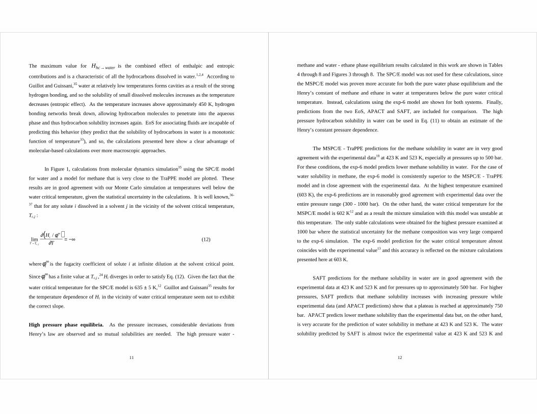
The maximum value for Hhc water→ is the combined effect of enthalpic and entropic

contributions and is a characteristic of all the hydrocarbons dissolved in water.1,2,4 According to

Guillot and Guissani,35 water at relatively low temperatures forms cavities as a result of the strong

hydrogen bonding, and so the solubility of small dissolved molecules increases as the temperature

decreases (entropic effect). As the temperature increases above approximately 450 K, hydrogen

bonding networks break down, allowing hydrocarbon molecules to penetrate into the aqueous

phase and thus hydrocarbon solubility increases again. EoS for associating fluids are incapable of

predicting this behavior (they predict that the solubility of hydrocarbons in water is a monotonic

function of temperature33), and so, the calculations presented here show a clear advantage of

molecular-based calculations over more macroscopic approaches.

In Figure 1, calculations from molecular dynamics simulation35 using the SPC/E model

for water and a model for methane that is very close to the TraPPE model are plotted. These

results are in good agreement with our Monte Carlo simulation at temperatures well below the

water critical temperature, given the statistical uncertainty in the calculations. It is well known,36-

37 that for any solute i dissolved in a solvent j in the vicinity of the solvent critical temperature,

Tc,j :

( )lim

/

,T T

i i

c j

H

T→

∞

= −∞∂ φ

∂(12)

whereφi∞ is the fugacity coefficient of solute i at infinite dilution at the solvent critical point.

Sinceφi∞ has a finite value at Tc,j ,

24 Hi diverges in order to satisfy Eq. (12). Given the fact that the

water critical temperature for the SPC/E model is 635 ± 5 K,12 Guillot and Guissani35 results for

the temperature dependence of Hi in the vicinity of water critical temperature seem not to exhibit

the correct slope.

High pressure phase equilibria. As the pressure increases, considerable deviations from

Henry’s law are observed and so mutual solubilities are needed. The high pressure water -

12

methane and water - ethane phase equilibrium results calculated in this work are shown in Tables

4 through 8 and Figures 3 through 8. The SPC/E model was not used for these calculations, since

the MSPC/E model was proven more accurate for both the pure water phase equilibrium and the

Henry’s constant of methane and ethane in water at temperatures below the pure water critical

temperature. Instead, calculations using the exp-6 model are shown for both systems. Finally,

predictions from the two EoS, APACT and SAFT, are included for comparison. The high

pressure hydrocarbon solubility in water can be used in Eq. (11) to obtain an estimate of the

Henry’s constant pressure dependence.

The MSPC/E - TraPPE predictions for the methane solubility in water are in very good

agreement with the experimental data18 at 423 K and 523 K, especially at pressures up to 500 bar.

For these conditions, the exp-6 model predicts lower methane solubility in water. For the case of

water solubility in methane, the exp-6 model is consistently superior to the MSPC/E - TraPPE

model and in close agreement with the experimental data. At the highest temperature examined

(603 K), the exp-6 predictions are in reasonably good agreement with experimental data over the

entire pressure range (300 - 1000 bar). On the other hand, the water critical temperature for the

MSPC/E model is 602 K12 and as a result the mixture simulation with this model was unstable at

this temperature. The only stable calculations were obtained for the highest pressure examined at

1000 bar where the statistical uncertainty for the methane composition was very large compared

to the exp-6 simulation. The exp-6 model prediction for the water critical temperature almost

coincides with the experimental value13 and this accuracy is reflected on the mixture calculations

presented here at 603 K.

SAFT predictions for the methane solubility in water are in good agreement with the

experimental data at 423 K and 523 K and for pressures up to approximately 500 bar. For higher

pressures, SAFT predicts that methane solubility increases with increasing pressure while

experimental data (and APACT predictions) show that a plateau is reached at approximately 750

bar. APACT predicts lower methane solubility than the experimental data but, on the other hand,

is very accurate for the prediction of water solubility in methane at 423 K and 523 K. The water

solubility predicted by SAFT is almost twice the experimental value at 423 K and 523 K and

13

relatively high pressure. Finally, at 603 K, SAFT is more accurate than APACT for the

composition in both phases.

The water - ethane phase equilibrium experimental and simulation data cover a much

broader pressure range, up to 3500 bar (Figures 6 through 8). Although at 523 K and 573 K

experimental data17 indicate a monotonic increase of ethane solubility with pressure, molecular

simulation using either of the two models predicts a maximum ethane solubility at approximately

500 bar for the MPSC/E - TraPPE model and 1000 - 1500 bar for the exp-6 model (Figures 6 and

7). A similar behavior is shown by APACT, which predicts maximum ethane solubility at 1000 -

1200 bar for the temperature range examined. The actual values for the ethane solubility in water

are very close for all three models. On the other hand, although SAFT qualitatively agrees with

the experimental data, the actual solubility values it predicts are 20 - 60 % higher than the

experimental ones.

For the water solubility in ethane at 523 K and 573 K, the exp-6 model is in better

agreement with the experimental data17 than the MSPC/E - TraPPE model, as is the case for water

in methane. APACT predictions are very close to the experimental data and exp-6 results,

whereas SAFT predictions are approximately twice the experimental values.

The phase diagram for water - ethane mixture at 623 K is qualitatively different than it is

at lower temperatures. At relatively low pressures, the mutual solubility of the two components

increases with pressure and at 680 bar the mixture becomes completely miscible (upper critical

solution pressure, UCSP). The mixture remains miscible up to 760 bar where a lower critical

solution pressure (LCSP) appears and the mixture becomes again immiscible. GEMC with the

exp-6 model predicts mutual solubilities at low pressure (below 500 bar) and high pressure

(above 1000 bar) that are in good agreement with the experimental data. Simulation in the

pressure range 500 - 1000 bar was unstable indicating that the model predicts complete

miscibility. It can be concluded therefore, that molecular simulation with an accurate molecular

model is able to predict this complex phase behavior.

14

On the other hand, APACT and SAFT predict that water and ethane are partially miscible

over the entire pressure range. SAFT predicts an hourglass behavior, which indicates that the two

components are miscible over a small pressure range at higher temperatures. These predictions

are due to the fact that both the APACT and SAFT critical temperatures for water are well above

the experimental value of 647.1 K.

It is quite remarkable that for both mixtures examined here and for conditions away from

the water critical point, APACT predictions are in close agreement with the simulation results

unlike SAFT, whose predictions deviate considerably from simulation. This agreement is more

pronounced for the hydrocarbon-rich phase (either methane or ethane). This behavior can be

attributed to the fact that APACT accounts for local composition effects through a second order

Lennard-Jones perturbation expansion, dipole-dipole perturbation expansion and asymmetric

mixing rules,32 whereas SAFT does not.31 In other words, APACT captures, even approximately,

all the interactions described on the molecular level by the different two-body molecular models

used in our simulations. The limitations of APACT are its inaccuracy for temperatures close to

one of the components critical point and for mixtures containing chain fluids. It is well known

that APACT does not have an accurate chain term. It simply predicts that the chain term of the

EoS can be calculated from the Carnahan-Starling expression for hard spheres multiplied by the

chain length.20 As a result, APACT becomes highly inaccurate for mixtures that contain chain

molecules such as heavy hydrocarbons.

Conclusions

In this work, the water - methane and water - ethane phase equilibria were examined from

approximately room temperature up to the critical point of water. Monte Carlo simulations were

compared to literature experimental data and EoS predictions. At relatively low pressure, Henry’s

law is a convenient way to describe the hydrocarbon solubility in water. The two molecular

models used, namely SPC/E and MSPC/E, were in good agreement with experimental data. As

the pressure increases, the mutual solubility increases substantially and the system is best

described by the compositions of the two coexisting phases. For these conditions, the GEMC

15

simulation method was used to predict the mixture phase equilibria using the MSPC/E and the

exp-6 models. In general, the results were in good agreement with experimental data. However,

because the exp-6 model is more accurate than the MSPC/E model in the vicinity of the pure

water critical point, water - methane simulations at 603 K were closer to the experimental data

using the exp-6 model than the MSPC/E model. Furthermore, the exp-6 model was able to

capture the very complex phase behavior of the water - ethane mixture at 623 K where a UCSP

and a LCSP are exhibited.

EoS predictions were in relatively good agreement with experimental data only at

temperatures well below the critical temperature of pure water. In addition, the EoS tested here

were specifically designed for associating fluids. When applied to other types of asymmetric

mixtures, for example mixtures of heavy hydrocarbons, they are significantly less accurate.38 By

contrast, molecular simulations of asymmetric hydrocarbon mixtures presented elsewhere38 are in

excellent agreement with experimental data, thus confirming the generality of the approach.

It was shown here clearly, that molecular simulation is a reliable tool for the calculation of

mixture phase equilibria of very dissimilar components such as water and hydrocarbons and for

conditions that are difficult to be reached experimentally, such as a few kbar of pressure. The

level of accuracy of the potential models for the prediction of pure component properties has a

direct effect on the accuracy for mixture predictions. Deviations between simulation and

experiment observed in this work can be possibly reduced by including in the potential models

explicitly the many body effects, such as polarizability effects, which are non-negligible for water

- hydrocarbon mixtures.39,40 The price to pay for such an increase in the accuracy of the

calculations will be the considerably higher computing time.40,41

16

Acknowledgments

We are grateful to Professor J.I. Siepmann, and Professor J.J. de Pablo for providing their

manuscripts prior to publication. The work at Cornell University and the University of Maryland

was supported by the National Science Foundation, under grant CTS-9509158. Partial financial

support of this project from NATO Collaborative Research Grants Programme under grant

number CRG 960966 is gratefully acknowledged.

17

References and Notes

(1) Tsonopoulos, C.; Wilson, G.M. AIChE J. 1983, 29, 990.

(2) Heidman, J.L.; Tsonopoulos, C.; Brady, C.J.; Wilson, G.M. AIChE J. 1985, 31, 376.

(3) Brunner, E. J. Chem. Thermodyn. 1990, 22, 335.

(4) Economou, I.G.; Heidman, J.L.; Tsonopoulos, C.; Wilson, G.M. AIChE J. 1997, 43, 535.

(5) Panagiotopoulos, A.Z. Mol. Phys. 1987, 61, 813.

(6) Panagiotopoulos, A.Z. In Supercritical Fluids - Fundamentals for Application, E. Kiran

and J.M.H. Levelt Sengers, eds.; Kluwer Academic Publishers: Dordrecht, 1994.

(7) Mehta, M.; Kofke, D.A. Chem. Eng. Sci. 1994, 49, 2633.

(8) Spyriouni, T.; Economou, I.G.; Theodorou, D.N. Macromolecules 1997, 30, 4744.

(9) Jorgensen, W.L.; Chandrasekhar, J.; Madura, J.D.; Impey R.W.; Klein, M.L. J. Chem.

Phys. 1983, 79, 926.

(10) Berendsen, H.J.C.; Postma, J.P.M.; van Gunsteren W.F.; Hermans, J. In Intermolecular

Forces, B. Pullman, ed.; Reidel: Dordrecht, 1981.

(11) Berendsen, H.J.C.; Grigera, J.R.; Straatsma, T.P. J. Phys. Chem. 1987, 91, 6269.

(12) Boulougouris, G.C.; Economou, I.G.; Theodorou, D.N. J.Phys. Chem. B 1998, 102, 1029.

(13) Errington, J.R.; Panagiotopoulos, A.Z. unpublished results 1998.

(14) Smit, B.; Karaborni, S.; Siepmann, J.I. J. Chem. Phys. 1995, 102, 2126.

(15) Nath, S.K.; Escobedo, F.A.; de Pablo, J.J. J. Chem. Phys. 1998, submitted.

(16) Martin, M.G.; Siepmann, J.I. J. Phys. Chem. 1998, submitted.

(17) Danneil, A.; Toedheide, K.; Franck, E.U. Chemie-Ing. Techn. 1967, 39, 816.

(18) Sultanov, R.G.; Skripka, V.G.; Yu, N.A. Zh. Fiz. Khim. 1972, 46, 2160.

(19) Harvey, A.H. AIChE J. 1996, 42, 1491.

(20) Ikonomou, G.D.; Donohue, M.D. AIChE J. 1986, 32, 1716.

(21) Huang, S.H.; Radosz, M. Ind. Eng. Chem. Res. 1990, 29, 2284.

(22) Bernal, J.D.; Fowler, R.H. J. Chem. Phys. 1933, 1, 515.

(23) Buckingham, R.A. Proc. Roy. Soc. 1938, 168A, 264.

(24) Prausnitz, J.M.; Lichtenthaler, R.N.; de Azevedo, E.G. Molecular Thermodynamics of Fluid-

Phase Equilibria, 2nd Ed.; Prentice-Hall: Englewood Cliffs, 1986.

18

(25) Widom, B. J. Chem. Phys. 1963, 39, 2808.

(26) Allen, M.P.; Tildesley, D.J. Computer Simulation of Liquids, Clarendon Press: Oxford, 1987.

(27) Siepmann J.I. Mol. Phys. 1990, 70, 1145.

(28) Frenkel, D.; Mooij, G.C.A.M.; Smit, B. J. Phys. Cond. Matt. 1992, 4, 3053.

(29) de Pablo, J.J.; Laso, M.; Suter, U.W. J. Chem. Phys. 1992, 96, 2395.

(30) Theodorou, D.N., Suter, U.W., J. Chem. Phys. 1985, 82, 955.

(31) Huang, S.H.; Radosz, M. Ind. Eng. Chem. Res. 1991, 30, 1994.

(32) Economou, I.G.; Peters, C.J.; de Swaan Arons, J. J. Phys. Chem. 1995, 99, 6182.

(33) Economou, I.G.; Tsonopoulos, C. Chem. Eng. Sci. 1997, 52, 511.

(34) Vimalchand, P.; Ikonomou, G.D.; Donohue, M.D. Fluid Phase Equil. 1988, 43, 121.

(35) Guillot, B.; Guissani, Y. J. Chem. Phys. 1993, 99, 8075.

(36) Beutier, D.; Renon, H. AIChE J. 1978, 24, 1122.

(37) Schotte, W. AIChE J. 1985, 31, 154.

(38) Spyriouni, T.; Economou, I.G.; Theodorou, D.N. Phys. Rev. Lett. 1997, submitted.

(39) Chialvo, A.A.; Cummings, P.T. J. Chem. Phys. 1996, 105, 8274.

(40) Kiyohara, K.; Gubbins, K.E.; Panagiotopoulos, A.Z. Mol. Phys. 1997, submitted.

(41) Ahlström, P.; Wallqvist, A.; Engström, S.; Jönsson, B. Mol. Phys. 1989, 68, 563.

19

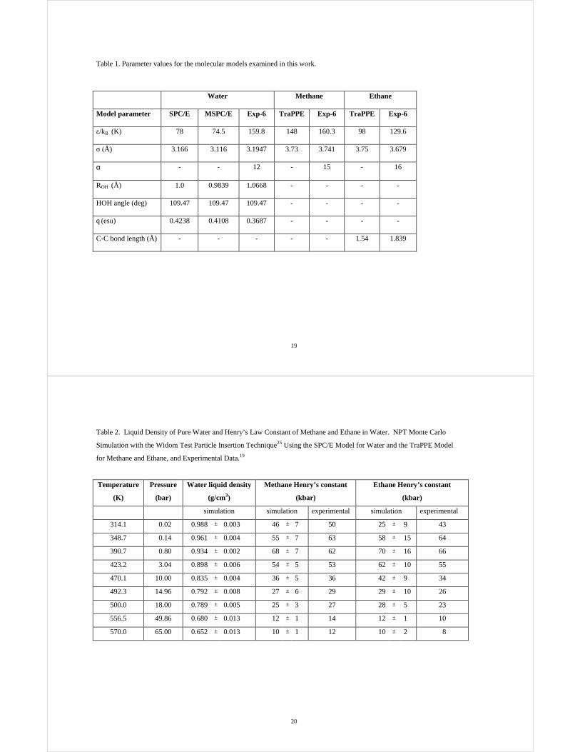
Table 1. Parameter values for the molecular models examined in this work.

Water Methane Ethane

Model parameter SPC/E MSPC/E Exp-6 TraPPE Exp-6 TraPPE Exp-6

0/kB (K) 78 74.5 159.8 148 160.3 98 129.6

1��Å) 3.166 3.116 3.1947 3.73 3.741 3.75 3.679

α - - 12 - 15 - 16

ROH (Å) 1.0 0.9839 1.0668 - - - -

HOH angle (deg) 109.47 109.47 109.47 - - - -

q (esu) 0.4238 0.4108 0.3687 - - - -

C-C bond length (Å) - - - - - 1.54 1.839

20

Table 2. Liquid Density of Pure Water and Henry’s Law Constant of Methane and Ethane in Water. NPT Monte Carlo

Simulation with the Widom Test Particle Insertion Technique25 Using the SPC/E Model for Water and the TraPPE Model

for Methane and Ethane, and Experimental Data.19

Temperature

(K)

Pressure

(bar)

Water liquid density

(g/cm3)

Methane Henry’s constant

(kbar)

Ethane Henry’s constant

(kbar)

simulation simulation experimental simulation experimental

314.1 0.02 0.988 ± 0.003 46 ± 7 50 25 ± 9 43

348.7 0.14 0.961 ± 0.004 55 ± 7 63 58 ± 15 64

390.7 0.80 0.934 ± 0.002 68 ± 7 62 70 ± 16 66

423.2 3.04 0.898 ± 0.006 54 ± 5 53 62 ± 10 55

470.1 10.00 0.835 ± 0.004 36 ± 5 36 42 ± 9 34

492.3 14.96 0.792 ± 0.008 27 ± 6 29 29 ± 10 26

500.0 18.00 0.789 ± 0.005 25 ± 3 27 28 ± 5 23

556.5 49.86 0.680 ± 0.013 12 ± 1 14 12 ± 1 10

570.0 65.00 0.652 ± 0.013 10 ± 1 12 10 ± 2 8

21

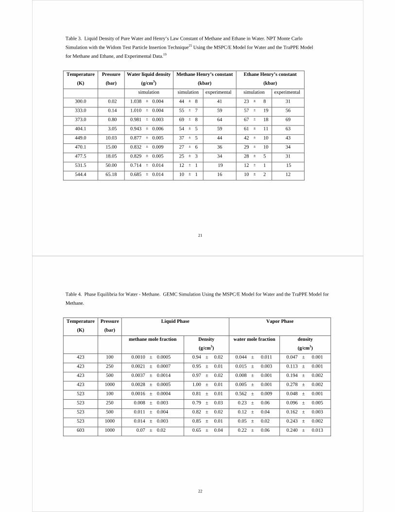
Table 3. Liquid Density of Pure Water and Henry’s Law Constant of Methane and Ethane in Water. NPT Monte Carlo

Simulation with the Widom Test Particle Insertion Technique25 Using the MSPC/E Model for Water and the TraPPE Model

for Methane and Ethane, and Experimental Data.19

Temperature

(K)

Pressure

(bar)

Water liquid density

(g/cm3)

Methane Henry’s constant

(kbar)

Ethane Henry’s constant

(kbar)

simulation simulation experimental simulation experimental

300.0 0.02 1.038 ± 0.004 44 ± 8 41 23 ± 8 31

333.0 0.14 1.010 ± 0.004 55 ± 7 59 57 ± 19 56

373.0 0.80 0.981 ± 0.003 69 ± 8 64 67 ± 18 69

404.1 3.05 0.943 ± 0.006 54 ± 5 59 61 ± 11 63

449.0 10.03 0.877 ± 0.005 37 ± 5 44 42 ± 10 43

470.1 15.00 0.832 ± 0.009 27 ± 6 36 29 ± 10 34

477.5 18.05 0.829 ± 0.005 25 ± 3 34 28 ± 5 31

531.5 50.00 0.714 ± 0.014 12 ± 1 19 12 ± 1 15

544.4 65.18 0.685 ± 0.014 10 ± 1 16 10 ± 2 12

22

Table 4. Phase Equilibria for Water - Methane. GEMC Simulation Using the MSPC/E Model for Water and the TraPPE Model for

Methane.

Temperature

(K)

Pressure

(bar)

Liquid Phase Vapor Phase

methane mole fraction Density

(g/cm3)

water mole fraction density

(g/cm3)

423 100 0.0010 ± 0.0005 0.94 ± 0.02 0.044 ± 0.011 0.047 ± 0.001

423 250 0.0021 ± 0.0007 0.95 ± 0.01 0.015 ± 0.003 0.113 ± 0.001

423 500 0.0037 ± 0.0014 0.97 ± 0.02 0.008 ± 0.001 0.194 ± 0.002

423 1000 0.0028 ± 0.0005 1.00 ± 0.01 0.005 ± 0.001 0.278 ± 0.002

523 100 0.0016 ± 0.0004 0.81 ± 0.01 0.562 ± 0.009 0.048 ± 0.001

523 250 0.008 ± 0.003 0.79 ± 0.03 0.23 ± 0.06 0.096 ± 0.005

523 500 0.011 ± 0.004 0.82 ± 0.02 0.12 ± 0.04 0.162 ± 0.003

523 1000 0.014 ± 0.003 0.85 ± 0.01 0.05 ± 0.02 0.243 ± 0.002

603 1000 0.07 ± 0.02 0.65 ± 0.04 0.22 ± 0.06 0.240 ± 0.013

23

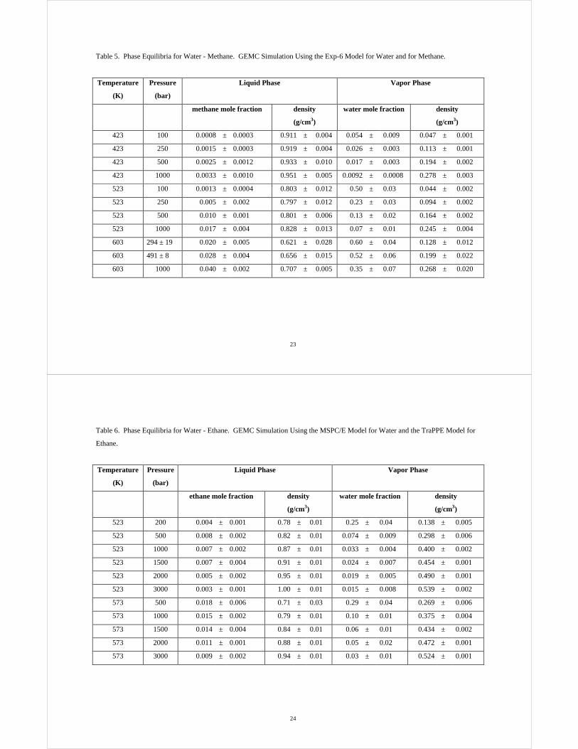
Table 5. Phase Equilibria for Water - Methane. GEMC Simulation Using the Exp-6 Model for Water and for Methane.

Temperature

(K)

Pressure

(bar)

Liquid Phase Vapor Phase

methane mole fraction density

(g/cm3)

water mole fraction density

(g/cm3)

423 100 0.0008 ± 0.0003 0.911 ± 0.004 0.054 ± 0.009 0.047 ± 0.001

423 250 0.0015 ± 0.0003 0.919 ± 0.004 0.026 ± 0.003 0.113 ± 0.001

423 500 0.0025 ± 0.0012 0.933 ± 0.010 0.017 ± 0.003 0.194 ± 0.002

423 1000 0.0033 ± 0.0010 0.951 ± 0.005 0.0092 ± 0.0008 0.278 ± 0.003

523 100 0.0013 ± 0.0004 0.803 ± 0.012 0.50 ± 0.03 0.044 ± 0.002

523 250 0.005 ± 0.002 0.797 ± 0.012 0.23 ± 0.03 0.094 ± 0.002

523 500 0.010 ± 0.001 0.801 ± 0.006 0.13 ± 0.02 0.164 ± 0.002

523 1000 0.017 ± 0.004 0.828 ± 0.013 0.07 ± 0.01 0.245 ± 0.004

603 294 ± 19 0.020 ± 0.005 0.621 ± 0.028 0.60 ± 0.04 0.128 ± 0.012

603 491 ± 8 0.028 ± 0.004 0.656 ± 0.015 0.52 ± 0.06 0.199 ± 0.022

603 1000 0.040 ± 0.002 0.707 ± 0.005 0.35 ± 0.07 0.268 ± 0.020

24

Table 6. Phase Equilibria for Water - Ethane. GEMC Simulation Using the MSPC/E Model for Water and the TraPPE Model for

Ethane.

Temperature

(K)

Pressure

(bar)

Liquid Phase Vapor Phase

ethane mole fraction density

(g/cm3)

water mole fraction density

(g/cm3)

523 200 0.004 ± 0.001 0.78 ± 0.01 0.25 ± 0.04 0.138 ± 0.005

523 500 0.008 ± 0.002 0.82 ± 0.01 0.074 ± 0.009 0.298 ± 0.006

523 1000 0.007 ± 0.002 0.87 ± 0.01 0.033 ± 0.004 0.400 ± 0.002

523 1500 0.007 ± 0.004 0.91 ± 0.01 0.024 ± 0.007 0.454 ± 0.001

523 2000 0.005 ± 0.002 0.95 ± 0.01 0.019 ± 0.005 0.490 ± 0.001

523 3000 0.003 ± 0.001 1.00 ± 0.01 0.015 ± 0.008 0.539 ± 0.002

573 500 0.018 ± 0.006 0.71 ± 0.03 0.29 ± 0.04 0.269 ± 0.006

573 1000 0.015 ± 0.002 0.79 ± 0.01 0.10 ± 0.01 0.375 ± 0.004

573 1500 0.014 ± 0.004 0.84 ± 0.01 0.06 ± 0.01 0.434 ± 0.002

573 2000 0.011 ± 0.001 0.88 ± 0.01 0.05 ± 0.02 0.472 ± 0.001

573 3000 0.009 ± 0.002 0.94 ± 0.01 0.03 ± 0.01 0.524 ± 0.001

25

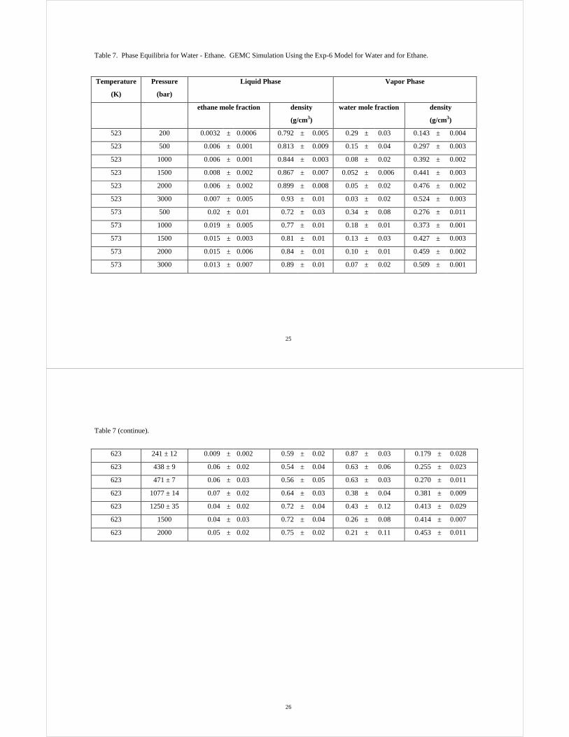
Table 7. Phase Equilibria for Water - Ethane. GEMC Simulation Using the Exp-6 Model for Water and for Ethane.

Temperature

(K)

Pressure

(bar)

Liquid Phase Vapor Phase

ethane mole fraction density

(g/cm3)

water mole fraction density

(g/cm3)

523 200 0.0032 ± 0.0006 0.792 ± 0.005 0.29 ± 0.03 0.143 ± 0.004

523 500 0.006 ± 0.001 0.813 ± 0.009 0.15 ± 0.04 0.297 ± 0.003

523 1000 0.006 ± 0.001 0.844 ± 0.003 0.08 ± 0.02 0.392 ± 0.002

523 1500 0.008 ± 0.002 0.867 ± 0.007 0.052 ± 0.006 0.441 ± 0.003

523 2000 0.006 ± 0.002 0.899 ± 0.008 0.05 ± 0.02 0.476 ± 0.002

523 3000 0.007 ± 0.005 0.93 ± 0.01 0.03 ± 0.02 0.524 ± 0.003

573 500 0.02 ± 0.01 0.72 ± 0.03 0.34 ± 0.08 0.276 ± 0.011

573 1000 0.019 ± 0.005 0.77 ± 0.01 0.18 ± 0.01 0.373 ± 0.001

573 1500 0.015 ± 0.003 0.81 ± 0.01 0.13 ± 0.03 0.427 ± 0.003

573 2000 0.015 ± 0.006 0.84 ± 0.01 0.10 ± 0.01 0.459 ± 0.002

573 3000 0.013 ± 0.007 0.89 ± 0.01 0.07 ± 0.02 0.509 ± 0.001

26

Table 7 (continue).

623 241 ± 12 0.009 ± 0.002 0.59 ± 0.02 0.87 ± 0.03 0.179 ± 0.028

623 438 ± 9 0.06 ± 0.02 0.54 ± 0.04 0.63 ± 0.06 0.255 ± 0.023

623 471 ± 7 0.06 ± 0.03 0.56 ± 0.05 0.63 ± 0.03 0.270 ± 0.011

623 1077 ± 14 0.07 ± 0.02 0.64 ± 0.03 0.38 ± 0.04 0.381 ± 0.009

623 1250 ± 35 0.04 ± 0.02 0.72 ± 0.04 0.43 ± 0.12 0.413 ± 0.029

623 1500 0.04 ± 0.03 0.72 ± 0.04 0.26 ± 0.08 0.414 ± 0.007

623 2000 0.05 ± 0.02 0.75 ± 0.02 0.21 ± 0.11 0.453 ± 0.011

27

Figure Captions

Figure 1. Henry’s law constant of methane in water. Experimental data (solid line),19 Monte

Carlo simulations using the SPC/E (open triangles) and MSPC/E (open squares) models for

water and the TraPPE model for methane calculated in this work and molecular dynamics

results (filled circles) from Guillot and Guissani.35

Figure 2. Henry’s law constant of ethane in water. Experimental data (solid line),19 and

Monte Carlo simulations using the SPC/E (open triangles) and MSPC/E (open squares)

models for water and the TraPPE model for ethane calculated in this work. The dashed line is

an extrapolation of the correlation proposed by Harvey.19

Figure 3. Water - methane high pressure phase equilibria at 423 K (top: liquid phase

composition; bottom: vapor phase composition). Experimental data (solid triangles),18

GEMC simulation with the MSPC/E - TraPPE model (open squares) and with the exp-6

model (open circles) and EoS predictions from APACT (dashed lines) and SAFT (solid lines).

Figure 4. Water - methane high pressure phase equilibria at 523 K (top: liquid phase

composition; bottom: vapor phase composition). Experimental data (solid triangles),18 GEMC

simulation with the MSPC/E - TraPPE model (open squares) and with the exp-6 model (open

circles) and EoS predictions from APACT (dashed lines) and SAFT (solid lines).

Figure 5. Water - methane high pressure phase equilibria at 603 K (top: liquid phase

composition; bottom: vapor phase composition). Experimental data (solid triangles),18 GEMC

simulation with the MSPC/E - TraPPE model (open squares) and with the exp-6 model (open

circles) and EoS predictions from APACT (dashed lines) and SAFT (solid lines).

Figure 6. Water - ethane high pressure phase equilibria at 523 K (top: liquid phase

composition; bottom: vapor phase composition). Experimental data (solid triangles),17 GEMC

simulation with the MSPC/E - TraPPE model (open squares) and with the exp-6 model (open

circles) and EoS predictions from APACT (dashed lines) and SAFT (solid lines).

28

Figure 7. Water - ethane high pressure phase equilibria at 573 K (top: liquid phase

composition; bottom: vapor phase composition). Experimental data (solid triangles),17 GEMC

simulation with the MSPC/E - TraPPE model (open squares) and with the exp-6 model (open

circles) and EoS predictions from APACT (dashed lines) and SAFT (solid lines).

Figure 8. Water - ethane high pressure phase equilibria at 623 K. Experimental data (solid

triangles),17 GEMC simulation with the exp-6 model (open circles) and EoS predictions from

APACT (dashed lines) and SAFT (solid lines).

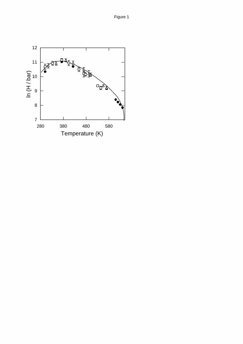
Figure 1

7

8

9

10

11

12

280 380 480 580

Temperature (K)

ln (

H /

bar)

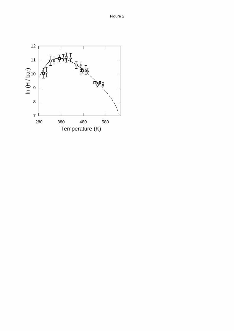
Figure 2

7

8

9

10

11

12

280 380 480 580

Temperature (K)

ln (

H /

bar)

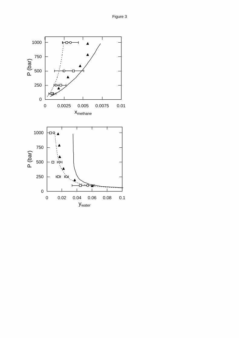
Figure 3

0

250

500

750

1000

0 0.02 0.04 0.06 0.08 0.1ywater

P (

bar)

0

250

500

750

1000

0 0.0025 0.005 0.0075 0.01

xmethane

P (

bar)

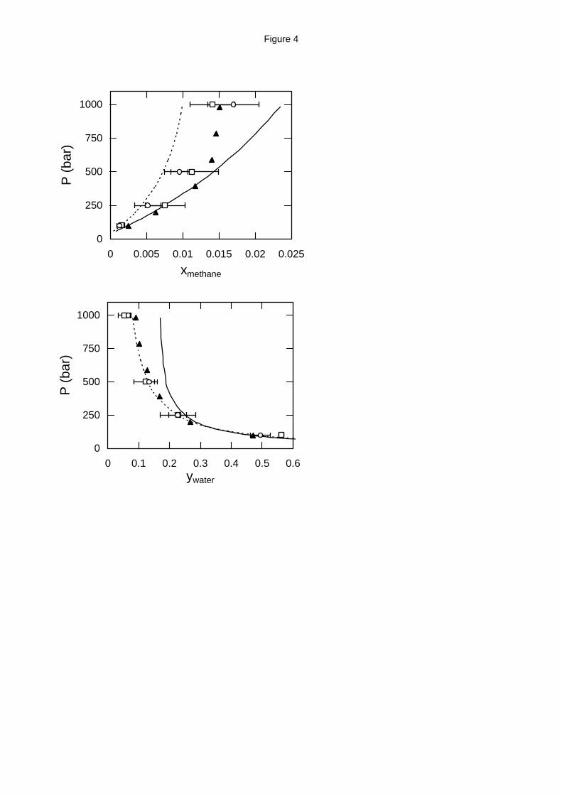
Figure 4

0

250

500

750

1000

0 0.1 0.2 0.3 0.4 0.5 0.6ywater

P (

bar)

0

250

500

750

1000

0 0.005 0.01 0.015 0.02 0.025

xmethane

P (

bar)

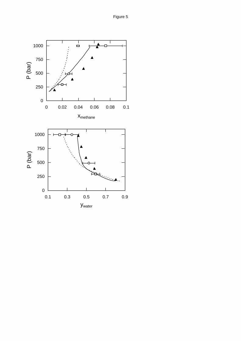
Figure 5

0

250

500

750

1000

0.1 0.3 0.5 0.7 0.9

ywater

P (

bar)

0

250

500

750

1000

0 0.02 0.04 0.06 0.08 0.1

xmethane

P (

bar)

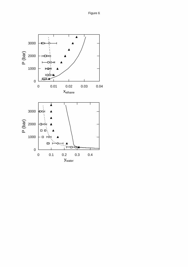
Figure 6

0

1000

2000

3000

0 0.1 0.2 0.3 0.4ywater

P (

bar)

0

1000

2000

3000

0 0.01 0.02 0.03 0.04

xethane

P (

bar)

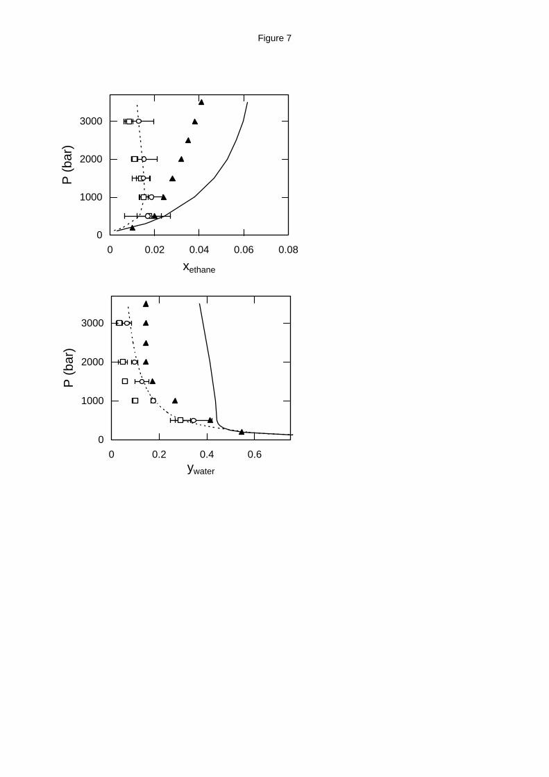
Figure 7

0

1000

2000

3000

0 0.2 0.4 0.6ywater

P (

bar)

0

1000

2000

3000

0 0.02 0.04 0.06 0.08

xethane

P (

bar)

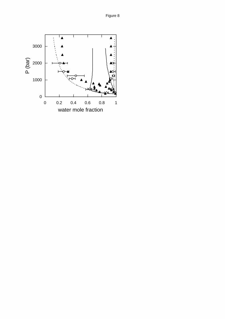
Figure 8

0

1000

2000

3000

0 0.2 0.4 0.6 0.8 1

water mole fraction

P (

bar)