Molecular Modeling:Molecular Modeling:Molecular MechanicsMolecular Mechanics

C372C372

Introduction to Introduction to Cheminformatics IICheminformatics II

Kelsey ForsytheKelsey Forsythe

Guidelines for UseGuidelines for Use

What systems were used to parameterizeWhat systems were used to parameterize How is energy calculatedHow is energy calculated What assumptions are used in the force What assumptions are used in the force

fieldfield How has it performed in the pastHow has it performed in the past

TransferabilityTransferability

AMBER (Assisted Model Building AMBER (Assisted Model Building Energy Refinement)Energy Refinement) Specific to proteins and nucleic acidsSpecific to proteins and nucleic acids

CHARMM (Chemistry at Harvard CHARMM (Chemistry at Harvard Macromolecular Mechanics)Macromolecular Mechanics) Specific to proteins and nucleic acids Specific to proteins and nucleic acids Widely used to model solvent effectsWidely used to model solvent effects Molecular dynamics integratorMolecular dynamics integrator

TransferabilityTransferability

MM? – (Allinger et. al.) MM? – (Allinger et. al.) Organic molecules Organic molecules

MMFF (Merck Molecular Force MMFF (Merck Molecular Force Field)Field) Organic moleculesOrganic molecules Molecular Dynamics Molecular Dynamics

Tripos/SYBYLTripos/SYBYL Organic and bio-organic moleculesOrganic and bio-organic molecules

TransferabilityTransferability

UFF (Universal Force Field)UFF (Universal Force Field) Parameters for all elements Parameters for all elements Inorganic systemsInorganic systems

YETI YETI Parameterized to model non-bonded Parameterized to model non-bonded

interactionsinteractions Docking (AmberDocking (AmberYETI)YETI)

How is Energy Calculated How is Energy Calculated

Valence TermsValence Terms Cross TermsCross Terms Non-bonding TermsNon-bonding Terms

Induced Dipole-Induced DipoleInduced Dipole-Induced Dipole Electrostatic/Ionic (Permanent Dipole) System not far Electrostatic/Ionic (Permanent Dipole) System not far

from equilibrium geometry (harmonic)from equilibrium geometry (harmonic) Energy is ? Energy is ?

Strain Energy (E=0 at equilibrium bond length/angle)Strain Energy (E=0 at equilibrium bond length/angle) Field Energy (Energy due to Non-bonding terms)Field Energy (Energy due to Non-bonding terms) Atomistic Heats of Formation (Parameterized so as to Atomistic Heats of Formation (Parameterized so as to

yield chemically meaningful values for yield chemically meaningful values for thermodynamics)thermodynamics)

K. Gilbert: This is only in the MM?-type force fieldsK. Gilbert: This is only in the MM?-type force fields

AssumptionsAssumptions

Hydrogens often not explicitly Hydrogens often not explicitly included (intrinsic hydrogen methods)included (intrinsic hydrogen methods) ““Methyl carbon” equated with 1 C and 3 Methyl carbon” equated with 1 C and 3

HsHs System not far from equilibrium System not far from equilibrium

geometry (harmonic)geometry (harmonic) Solvent is vacuum or simple dielectricSolvent is vacuum or simple dielectric

Modeling Potential energyModeling Potential energy

€

U(r) U(req ) −dU

dr r= req

(r − req ) +1

2

d2U

dr2

r= req

(r − req )2

€

−1

3

d3U

drr= req

(r − req )3 ....+1

n!

dnU

drn

r= req

(r − req )n€

=

€

≈

Modeling Potential energyModeling Potential energy

€

−dU

dr r= req

(r − req ) +

€

U(r) ≈1

2

d2U

dr2

r= req

(r − req )2 ≡1

2kAB (r − req )2

€

U(req )

€

U(r) 1

2

d2U

dr2

r= req

(r − req )2

€

≈

0 at minimum0

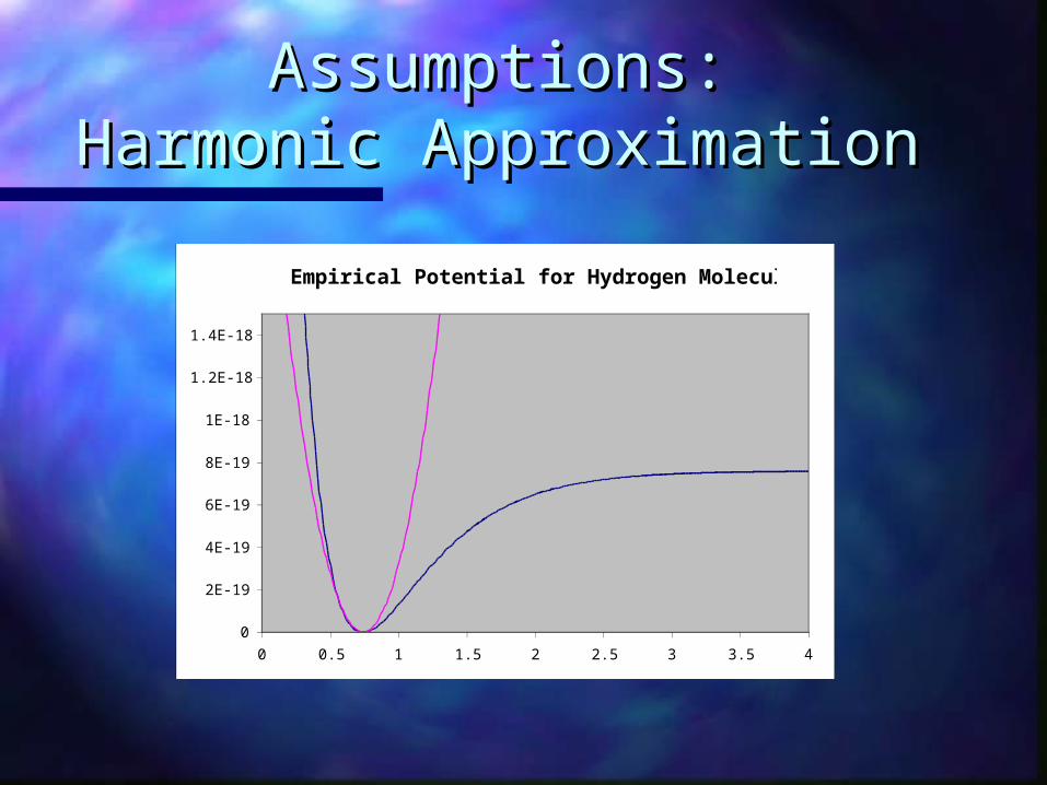
Assumptions:Assumptions:Harmonic ApproximationHarmonic Approximation

8.35E-28 8.77567E+14 20568787140 2.03098E-18 1.05374E-188.35E-28 8.77567E+14 20568787140 1.77569E-18 9.66155E-198.35E-28 8.77567E+14 20568787140 1.54682E-18 8.82365E-198.35E-28 8.77567E+14 20568787140 1.34201E-18 8.02375E-198.35E-28 8.77567E+14 20568787140 1.15913E-18 7.26185E-198.35E-28 8.77567E+14 20568787140 9.96207E-19 6.53795E-198.35E-28 8.77567E+14 20568787140 8.51451E-19 5.85205E-198.35E-28 8.77567E+14 20568787140 7.23209E-19 5.20415E-198.35E-28 8.77567E+14 20568787140 6.09973E-19 4.59425E-198.35E-28 8.77567E+14 20568787140 5.10362E-19 4.02235E-198.35E-28 8.77567E+14 20568787140 4.2311E-19 3.48845E-198.35E-28 8.77567E+14 20568787140 3.47061E-19 2.99255E-198.35E-28 8.77567E+14 20568787140 2.81155E-19 2.53465E-198.35E-28 8.77567E+14 20568787140 2.24426E-19 2.11475E-198.35E-28 8.77567E+14 20568787140 1.75987E-19 1.73285E-198.35E-28 8.77567E+14 20568787140 1.35031E-19 1.38895E-198.35E-28 8.77567E+14 20568787140 1.0082E-19 1.08305E-198.35E-28 8.77567E+14 20568787140 7.26787E-20 8.15147E-208.35E-28 8.77567E+14 20568787140 4.99924E-20 5.85247E-208.35E-28 8.77567E+14 20568787140 3.22001E-20 3.93347E-208.35E-28 8.77567E+14 20568787140 1.87901E-20 2.39447E-208.35E-28 8.77567E+14 20568787140 9.29638E-21 1.23547E-208.35E-28 8.77567E+14 20568787140 3.29443E-21 4.56475E-21

Empirical Potential for Hydrogen Molecule

0

2E-19

4E-19

6E-19

8E-19

1E-18

1.2E-18

1.4E-18

0 0.5 1 1.5 2 2.5 3 3.5 4

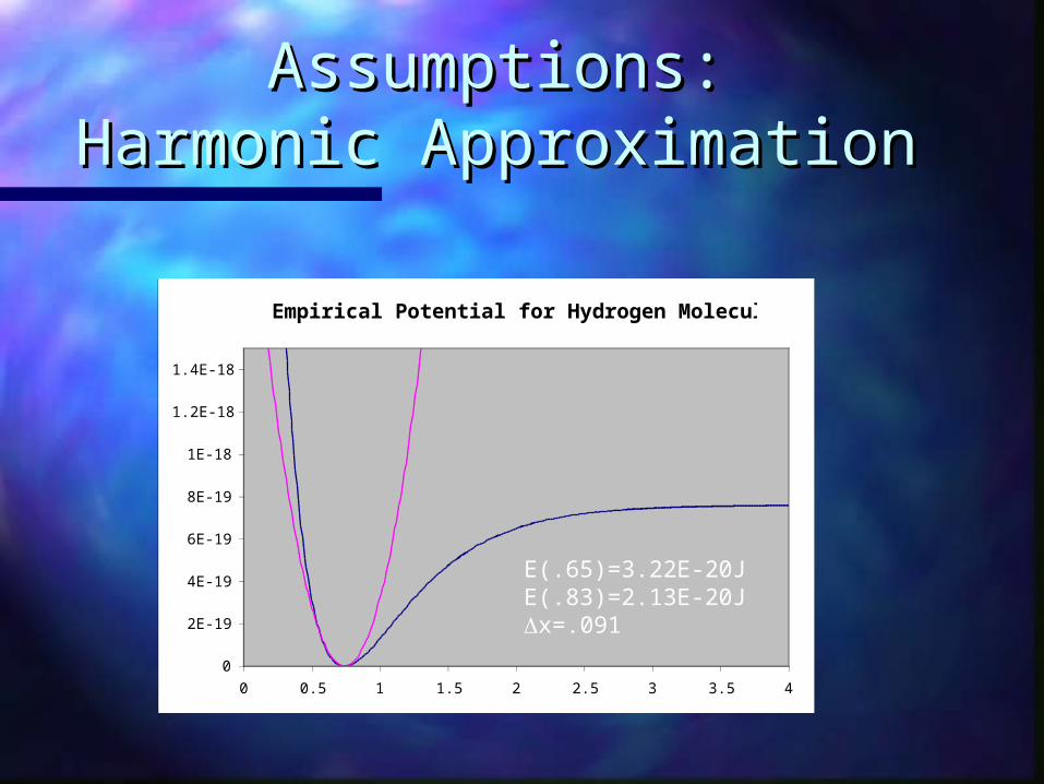
Assumptions:Assumptions:Harmonic ApproximationHarmonic Approximation

Determining k?

€

E(x0 − Δx) ≅ E(x0) +1

2

d2U

dx 2

x0

((x0 − Δx) − x0)2

E(x0 + Δx) ≅ E(x0) +1

2

d2U

dx 2

x0

((x0 + Δx) − x0)2

d2U

dx 2

x0

≅E(x0 − Δx) + E(x0 + Δx) − 2E(x0)

(Δx)2

8.35E-28 8.77567E+14 20568787140 2.03098E-18 1.05374E-188.35E-28 8.77567E+14 20568787140 1.77569E-18 9.66155E-198.35E-28 8.77567E+14 20568787140 1.54682E-18 8.82365E-198.35E-28 8.77567E+14 20568787140 1.34201E-18 8.02375E-198.35E-28 8.77567E+14 20568787140 1.15913E-18 7.26185E-198.35E-28 8.77567E+14 20568787140 9.96207E-19 6.53795E-198.35E-28 8.77567E+14 20568787140 8.51451E-19 5.85205E-198.35E-28 8.77567E+14 20568787140 7.23209E-19 5.20415E-198.35E-28 8.77567E+14 20568787140 6.09973E-19 4.59425E-198.35E-28 8.77567E+14 20568787140 5.10362E-19 4.02235E-198.35E-28 8.77567E+14 20568787140 4.2311E-19 3.48845E-198.35E-28 8.77567E+14 20568787140 3.47061E-19 2.99255E-198.35E-28 8.77567E+14 20568787140 2.81155E-19 2.53465E-198.35E-28 8.77567E+14 20568787140 2.24426E-19 2.11475E-198.35E-28 8.77567E+14 20568787140 1.75987E-19 1.73285E-198.35E-28 8.77567E+14 20568787140 1.35031E-19 1.38895E-198.35E-28 8.77567E+14 20568787140 1.0082E-19 1.08305E-198.35E-28 8.77567E+14 20568787140 7.26787E-20 8.15147E-208.35E-28 8.77567E+14 20568787140 4.99924E-20 5.85247E-208.35E-28 8.77567E+14 20568787140 3.22001E-20 3.93347E-208.35E-28 8.77567E+14 20568787140 1.87901E-20 2.39447E-208.35E-28 8.77567E+14 20568787140 9.29638E-21 1.23547E-208.35E-28 8.77567E+14 20568787140 3.29443E-21 4.56475E-21

Empirical Potential for Hydrogen Molecule

0

2E-19

4E-19

6E-19

8E-19

1E-18

1.2E-18

1.4E-18

0 0.5 1 1.5 2 2.5 3 3.5 4

Assumptions:Assumptions:Harmonic ApproximationHarmonic Approximation

E(.65)=3.22E-20JE(.83)=2.13E-20Jx=.091

Assumptions:Assumptions:Harmonic ApproximationHarmonic Approximation

€

d2U

dx 2

x0

≅E(x0 − Δx) + E(x0 + Δx) − 2E0

Δx 2

d2U

dx 2

x0

=(3.22 ×10−20 J) + (2.126 ×10−20 J)

(.091A ×1m

1×1010 A)2

d2U

dx 2

x0

= 6.45 ×102 kg

s2≡ k

Assumptions:Assumptions:Harmonic ApproximationHarmonic Approximation

€

d2U

dx 2

x0

= 6.45 ×102 kg

s2≡ k

HO − −− > k = mω2

∴ ω =k

μ=

6.45 ×102 kg

s2

1.67 ×10−27 kg= 6.215 ×1014 Hz

ν =ω

2π= 9.891×1013 Hz ≡ 3.30 ×103cm−1(Exp : 4.395 ×103cm−1)

AssumptionsAssumptions

Hydrogens often not explicitly Hydrogens often not explicitly included (intrinsic hydrogen methods)included (intrinsic hydrogen methods) ““Methyl carbon” equated with 1 C and 3 Methyl carbon” equated with 1 C and 3

HsHs System not far from equilibrium System not far from equilibrium

geometry (harmonic)geometry (harmonic) Solvent is vacuum or simple dielectricSolvent is vacuum or simple dielectric

Assumptions:Assumptions:solvent effectssolvent effects

Christensen, O. B. et. al, Phys. Rev. B. 40, 1993 (1989)

H2 in Pd

DFT

Empirical Potentials for Hydrogen Molecule

0

1

2

3

4

5

6

7

8

9

10

0 0.5 1 1.5 2 2.5

Intermolecular/atomic Intermolecular/atomic modelsmodels

General form:General form:

Lennard-Jones Lennard-Jones

€

V = V (r) + V (ri,rj ) + V (ri,rj ,rk ) + .....i< jj<k

N

∑i< j

N

∑

€

V (rij ) = 4εσ

r

⎛

⎝ ⎜

⎞

⎠ ⎟

12

1 2 3 −

σ

r

⎛

⎝ ⎜

⎞

⎠ ⎟6 ⎡

⎣ ⎢

⎤

⎦ ⎥

1 2 3

⎡

⎣

⎢ ⎢ ⎢ ⎢

⎤

⎦

⎥ ⎥ ⎥ ⎥

Van derWaals repulsionVan derWaals repulsion London AttractionLondon Attraction

0at which distance

depth well

=−−

ABVσε

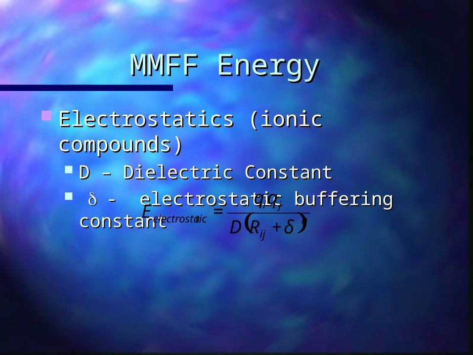
MMFF EnergyMMFF Energy

Electrostatics (ionic compounds) Electrostatics (ionic compounds) D – Dielectric ConstantD – Dielectric Constant - electrostatic buffering constant- electrostatic buffering constant

( )nij

jiticelectrosta

RD

qqE

δ+=

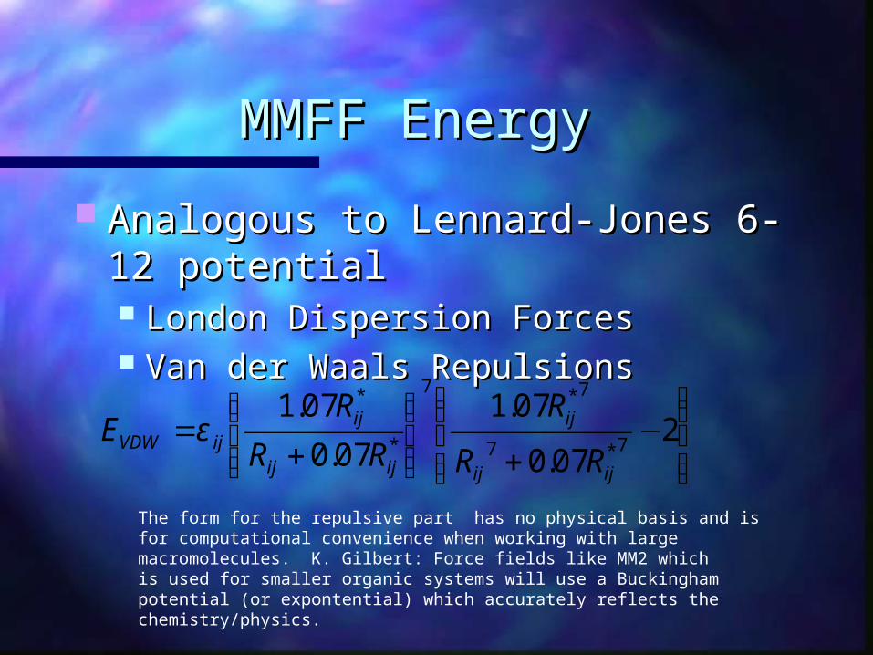
MMFF EnergyMMFF Energy

Analogous to Lennard-Jones 6-12 Analogous to Lennard-Jones 6-12 potentialpotential London Dispersion ForcesLondon Dispersion Forces Van der Waals RepulsionsVan der Waals Repulsions

⎪⎭

⎪⎬⎫

⎪⎩

⎪⎨⎧

−+⎪⎭

⎪⎬⎫

⎪⎩

⎪⎨⎧

+= 2

07.0

07.1

07.0

07.17*7

7*7

*

*

ijij

ij

ijij

ijijVDW

RR

R

RR

RE ε

The form for the repulsive part has no physical basis and is for computational convenience when working with largemacromolecules. K. Gilbert: Force fields like MM2 which is used for smaller organic systems will use a Buckingham potential (or expontential) which accurately reflects the chemistry/physics.

Pros and ConsPros and Cons

N >> 1000 atomsN >> 1000 atoms Easily Easily

constructedconstructed

AccuracyAccuracy Not robust enough Not robust enough

to describe subtle to describe subtle chemical effectschemical effects HydrophobicityHydrophobicity Excited StatesExcited States RadicalsRadicals

Does not Does not reproduce quantal reproduce quantal naturenature

CaveatsCaveats

Compare energy differences NOT energiesCompare energy differences NOT energies Always compare results with higher order Always compare results with higher order

theory (theory (ab initioab initio) and/or experiments) and/or experiments