MOLECULAR DYNAMICS SIMULATION OF THE THERMAL

PROPERTIES OF Y-JUNCTION CARBON NANOTUBES

By

ARON WILLIAM CUMMINGS

A thesis submitted in partial fulfillment of the requirements for the degree of

MASTER OF SCIENCE IN ELECTRICAL ENGINEERING

WASHINGTON STATE UNIVERSITY Department of Electrical Engineering and Computer Science

August 2004

ii

To the Faculty of Washington State University:

The members of the Committee appointed to examine the thesis of ARON WILLIAM CUMMINGS find it satisfactory and recommend that it be accepted.

___________________________________ Chair ___________________________________ ___________________________________

iii

ACKNOWLEDGEMENTS

Aron Cummings would like to acknowledge the financial support of a graduate

fellowship from Washington State University’s school of Electrical Engineering and Computer

Science, and of the Department of Energy’s Computational Science Graduate Fellowship

provided under grant number DE-FG02-97ER25308. He would also like to acknowledge

support provided by Deepak Srivastava through a NASA Ames Education Associates summer

internship at NASA’s Ames Research Center. He would like to thank his committee members,

Dr. Pedrow and Dr. McCluskey, for their input. Finally, he would like to acknowledge the

significant counsel provided by his advisor, Dr. Mohamed Osman.

iv

MOLECULAR DYNAMICS SIMULATION OF THE THERMAL

PROPERTIES OF Y-JUNCTION CARBON NANOTUBES

Abstract

by Aron William Cummings, M.S. Washington State University

August 2004 Chair: Mohamed A. Osman Molecular dynamics simulations have been used to investigate the thermal properties of a

Y-junction carbon nanotube consisting of a (14,0) trunk splitting into a pair of (7,0) branches.

Steady state simulations were used to calculate the thermal conductivity of the Y-junction

nanotube over a range of temperatures. It was found that the thermal conductivity of the Y-

junction nanotube is less than that of a corresponding straight (14,0) nanotube, due to lattice

defects in the form of non-hexagonal carbon rings at the junction. These lattice defects result in

a discontinuity in the temperature profile of the Y-junction nanotube. Defects that were

introduced to a straight (14,0) nanotube resulted in a similar discontinuity in the temperature

profile. Phonon spectra revealed that the presence of lattice defects suppresses the density of

certain vibration modes, which in turn impedes the heat flow.

Heat pulse simulations were also conducted on the Y-junction nanotube. These revealed

that the junction at least partially blocked all propagating modes. Furthermore, some asymmetry

in heat flow was observed. Traveling waves passed well from the trunk to the branches, but not

vice versa. This was attributed the vibrations in traveling waves in the branches being out of

phase when they reach the junction. Finally, the inconsistencies in the magnitude and stability of

v

the waves generated by the heat pulse were attributed to variations in the initial state of the

carbon nanotube that get blown up when the heat pulse is applied.

vi

TABLE OF CONTENTS 1 INTRODUCTION 1

2 CARBON NANOTUBES 3

2.1. Introduction …………………………………………….……………………….. 3

2.2. Physical Structure ………………………………………………………………. 3

2.3. Electrical Properties …………………………………………………………….. 6

2.4. Thermal Properties ……………………………………………………………… 10

3 MOLECULAR DYNAMICS 14

3.1. Introduction ……………………………………………………………………... 14

3.2. General Method ………………………………………………………………… 14

3.3. The Tersoff-Brenner Interatomic Potential ……………………………………... 17

3.4. The Nordsieck-Gear Predictor-Corrector Method ……………………………… 18

3.5. Calculation of System Properties ……………………………………………….. 20

3.5.1. Kinetic Energy ………………………………………………………….. 20

3.5.2. Temperature …………………………………………………………….. 20

3.5.3. Velocity Autocorrelation Function ……………………………………... 21

3.5.4. Thermal Conductivity …………………………………………………... 24

4 STEADY STATE HEAT FLOW 25

4.1. Introduction ……………………………………………………………………... 25

4.2. Methodology ……………………………………………………………………. 25

4.3. Results …………………………………………………………………………... 30

4.4. Discussion ………………………………………………………………………. 38

5 HEAT PULSE PROPAGATION 40

vii

5.1. Introduction ……………………………………………………………………... 40

5.2. Methodology ……………………………………………………………………. 40

5.3. Results …………………………………………………………………………... 42

5.4. Discussion ………………………………………………………………………. 49

6 CONCLUSION 54

REFERENCES 56

viii

LIST OF FIGURES

2.1. The unrolled hexagonal lattice of a nanotube .………………………………………. 4

2.2. Three geometries of carbon nanotubes .……………………………………………... 5

2.3. Example Y-junction configurations …………………………………………………. 6

2.4. Reciprocal lattice diagram of 2D graphite and a carbon nanotube ………………….. 7

2.5. Some geometries of carbon nanotubes and their resulting electrical configuration .... 8

2.6. Qualitative temperature dependence of the thermal conductivity of crystals ……….. 11

3.1. High-level process of molecular dynamics simulation ……………………………… 17

3.2. Velocity autocorrelation function of a (14,0) carbon nanotube .…………………….. 23

4.1. Molecular dynamics setup for calculating the thermal conductivity of a straight

carbon nanotube. The ellipses indicate that periodic boundary conditions are

applied ……………………………………………………………………………….. 26

4.2. Molecular dynamics setup for calculating the thermal conductivity of the

Y-junction nanotube .………………………………………………………………... 28

4.3. Temperature dependence of the thermal conductivity. The squares represent the

straight (14,0) nanotube, the triangles represent the forward heat flow configuration

of the y-junction tube, and the circles represent the reverse heat flow configuration

of the y-junction tube .……………………………………………………………….. 31

4.4. Temperature dependence of the heat flux density. The squares represent the straight

(14,0) nanotube, the triangles represent the forward heat flow configuration of the

y-junction tube, and the circles represent the reverse heat flow configuration of the

y-junction tube ………………………………………………………………………. 32

4.5. Temperature dependence of the temperature gradient. The squares represent the

straight (14,0) nanotube, the triangles represent the forward heat flow configuration

ix

of the y-junction tube, and the circles represent the reverse heat flow configuration

of the y-junction tube .………………………………………...……………………... 33

4.6. Temperature profiles of (a) the straight (14,0) nanotube, (b) the Y-junction

nanotube, (c) the straight (14,0) nanotube with vacancy defects, and (d) the straight

(14,0) nanotube with a Stone-Wales (5,7,7,5) defect. Fit lines have been added to

show the slope in each region .………………………………………...…………….. 34

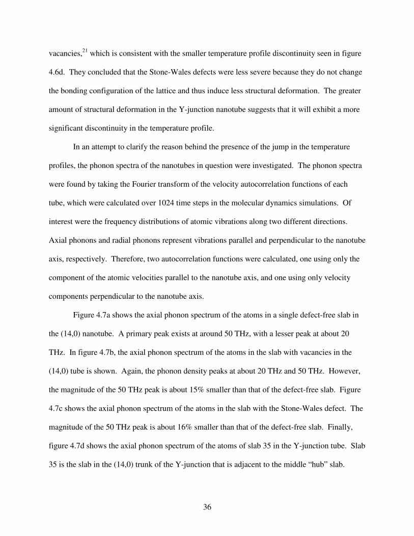
4.7. Axial phonon spectra of (a) the straight (14,0) nanotube, (b) the straight

(14,0) tube slab with vacancy defects, (c) the straight (14,0) nanotube slab

with a Stone-Wales (5,7,7,5) defect, and (d) Y-junction slab 35. These

spectra represent atomic vibrations parallel to the tube axis .……………………….. 37

5.1. Molecular dynamics setup for applying a heat pulse to the Y-junction

carbon nanotube .…………………………………………………………………….. 41

5.2. Time-dependent behavior of the applied heat pulse .………………………………... 41

5.3. Heat pulse results of the (7,0) carbon nanotube .……………………………………. 44

5.4. Heat pulse results of the (14,0) carbon nanotube .…………………………………… 46

5.5. Heat pulse results of the Y-junction carbon nanotube with the pulse applied to both

branches simultaneously …………………….………………………………………. 48

5.6. Heat pulse results of the Y-junction carbon nanotube with the pulse applied to one

branch ………………………………………………………………………………...50

5.7. Heat pulse results of the Y-junction carbon nanotube with the pulse applied to the

trunk ……...………………………………………………………………………….. 51

x

Dedication

I would like to thank my family,

who only expected my best.

1

CHAPTER ONE

INTRODUCTION

Computers today are constructed with a technology known as Complementary Metal-

Oxide-Semiconductor (CMOS) technology, which consists of a network of field-effect

transistors patterned onto a silicon wafer using lithographic techniques. The incredible

improvements made in this technology over the past several decades are due primarily to the

progression of fabrication techniques that allow for CMOS devices to be created at ever-smaller

dimensions. Today, these devices have features that can be measured on the scale of tens to

hundreds of nanometers. However, the problems with fabricating devices on these scales make it

apparent that CMOS devices cannot grow much smaller. Therefore, researchers are attempting

to identify a new type of technology that will allow the construction of devices that can be

measured on the single-nanometer scale. This exploding area of research is known as

nanotechnology.1

One of the linchpins of the nanotechnology industry today is the carbon nanotube.

Discovered in 1991,2 the carbon nanotube is a hollow cylinder made entirely of carbon atoms

with a radius that can reach less than one nanometer. Shortly after their discovery, several

studies were undertaken to determine the electrical properties of these new structures. It was

found that some nanotubes are metallic in nature, while others are semiconductors, and that this

depends entirely on their chirality.3 Furthermore, it was found that the band gap of the

semiconducting nanotubes is inversely proportional to their radius.4 Studies of the thermal

properties of carbon nanotubes have revealed them to be some of the best thermal conductors

known.5

2

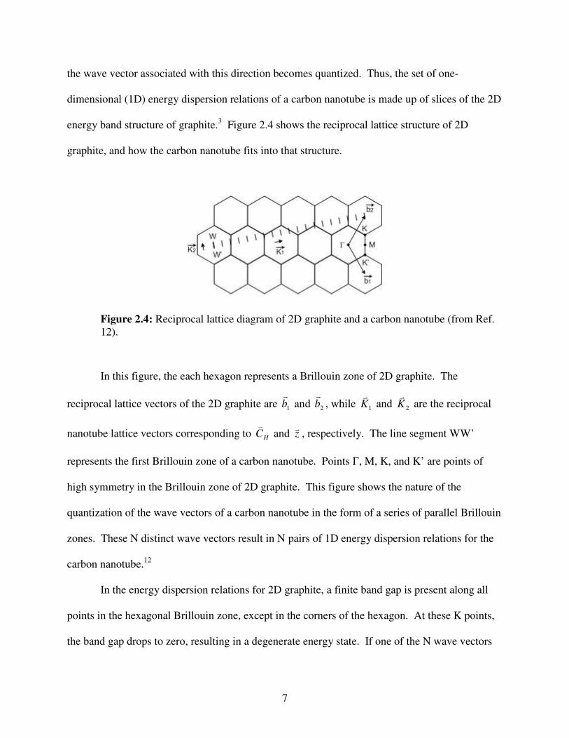
The diameter-dependence of the band gap of the semiconducting nanotubes has led

researchers to propose and investigate a variety of structures that involve the connection of one

nanotube to another. Some of these structures include T-junctions,6 Y-junctions,7 and X-

junctions.8 Later, Y-junctions of multi-wall carbon nanotubes were fabricated using a template-

based approach that allows the fabrication of many Y-junctions in a single experiment.9

Theoretical10 and experimental11 studies on Y-junction nanotubes have revealed that they behave

as electrical rectifiers, much like a diode. However, up to this point no studies on the thermal

properties of these structures have been undertaken.

Given their interesting electrical properties and the fact that they can be fabricated in

large bundles, it seems important to characterize these Y-junction structures as much as possible.

Therefore, the goal of the research described in this thesis is to study the thermal properties of Y-

junction carbon nanotubes. To do this, a molecular dynamics approach has been chosen.

Molecular dynamics is a method of simulation that determines the time evolution of a set of

interacting atoms by integrating their equations of motion. This approach is considered to be

classical because the equations of motion are none other than Newton’s law, iii amF��

= , for each

atom i in a system of N atoms. Because this simulation method provides information about the

motion of each atom, it is a good one for calculating a variety of thermal properties.

This thesis is organized into six chapters. Chapter 2 describes the structure, electrical and

thermal properties of straight and Y-junction carbon nanotubes. A detailed explanation of

molecular dynamics can be found in Chapter 3. Chapter 4 describes the methodology and results

of steady state heat flow through a Y-junction carbon nanotube. The procedure and results of

heat pulse propagation through a Y-junction carbon nanotube are provided in Chapter 5, and

conclusions are presented in Chapter 6.

3

CHAPTER TWO

CARBON NANOTUBES

2.1. Introduction

The growth of carbon nanotubes was first accomplished and reported by Sumio Iijima in

1991.2 Since that time, a significant amount of effort has been put into the theoretical and

experimental study of these structures. The purpose of this chapter is to provide some

background information on carbon nanotubes, which will aid in the understanding of subsequent

chapters. Specifically, this chapter will discuss the physical structure of straight and Y-junction

carbon nanotubes and their resulting electrical and thermal properties.

2.2. Physical Structure

A single-wall carbon nanotube can be viewed as a single sheet of graphite rolled up into a

cylinder. Figure 2.1 shows a representation of the 2D hexagonal plane that makes up a graphitic

sheet, where the carbon atoms lie at the corners of each hexagon. In this figure, one can see that

if point O is connected to point A, and point B is connected to point B’, then the sheet will be

rolled into a cylindrical structure. However, this is just one of many possible cylindrical

orientations that can be constructed. For example, points A and B’ could lay directly to the right

of points O and B, respectively, which would result in a different orientation of the hexagonal

rings on the face of the cylinder.12

The vector HC�

, known as the “chiral” vector, is that which uniquely determines the

physical structure of a carbon nanotube, and is perpendicular to the tube axis z� . HC�

can be

written in terms of the unit vectors of the hexagonal lattice, 1a� and 2a� , such that

4

Figure 2.1: The unrolled hexagonal lattice of a nanotube (from Ref. 12).

21 amanCH���

+= . Thus, the integer pair (n,m) is used to completely describe the geometry of a

carbon nanotube. Because of the rotational symmetry of the 2D hexagonal lattice, it is only

necessary to consider n and m such that nm ≤≤0 . In the case that m = n, the angle � will be

30o. In this case, as one moves along the chiral vector, the carbon bonds form an armchair-

shaped pattern. Thus, a carbon nanotube of the form (n,n) is known as an armchair nanotube. In

the case that m = 0, � = 0o and the bonds along the chiral vector form a zigzag pattern. So,

carbon nanotubes of the form (n,0) are known as zigzag nanotubes. In all other cases, 0o < � <

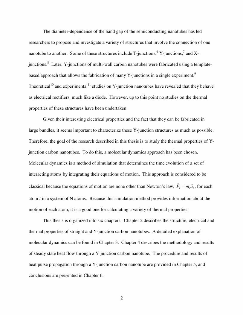
30o, and the tubes are known as chiral nanotubes. Figure 2.2 shows an example of each of the

three different types of carbon nanotubes.12 Note the zigzag and armchair patterns at the end

rings of the zigzag and arm chair carbon nanotubes. In figure 2.2, all three nanotubes are single-

wall carbon nanotubes. There also exist multi-wall carbon nanotubes, which consist of two or

more concentric single-wall carbon nanotubes. The focus of study in this research is on single-

wall carbon nanotubes.

5

Figure 2.2: Three geometries of carbon nanotubes (from Ref. 12).

The structure of interest in this research, the Y-junction carbon nanotube, was first

proposed in 1998.7 The Y-junction structure consists of a single “trunk” nanotube splitting into

two “branch” nanotubes. Figure 2.3 below shows some examples of Y-junction configurations.

The structure of the trunk and branches of the Y-junction nanotube is the same as that for a

straight single-wall carbon nanotube. The difference in structure lies at the junction, where the

continuity of the hexagonal lattice cannot be conserved. To realize the Y-junction, non-

hexagonal polygons with 4, 5, 7, or 8 edges must be introduced into the lattice. The number of

extra edges introduced into the lattice is known as the bond surplus. Thus, an octagon

contributes a bond surplus of +2, while a pentagon contributes a bond surplus of -1. Through an

application of Euler’s rule for polygons on the surface of a closed polyhedron, Crespi proposed a

6

rule for the bond surplus of carbon nanotube junctions.13 His rule was that a junction consisting

of N tubes would have a bond surplus of 12(N-2). Thus, a Y-junction should have a bond

surplus of 12. However, this surplus can be shared between the two junctions, resulting in a need

for 6 extra polygonal edges.13 In figure 2.3 above, the two Y-junctions on the left contain 6

heptagons, while the one on the right contains 4 heptagons and an octagon.10

Figure 2.3: Example Y-junction configurations (from Ref. 10).

2.3. Electrical Properties

Soon after their synthesis in 1991, several theoretical studies were undertaken to

determine the electrical nature of carbon nanotubes.3,4,14 These studies found that the electronic

structure of carbon nanotubes can be determined starting from that of two-dimensional (2D)

graphite. When a plane of graphite is rolled up into a carbon nanotube, periodic boundary

conditions are imposed in the circumferential direction described by the chiral vector HC�

, and

7

the wave vector associated with this direction becomes quantized. Thus, the set of one-

dimensional (1D) energy dispersion relations of a carbon nanotube is made up of slices of the 2D

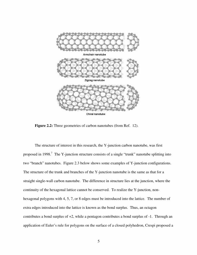
energy band structure of graphite.3 Figure 2.4 shows the reciprocal lattice structure of 2D

graphite, and how the carbon nanotube fits into that structure.

Figure 2.4: Reciprocal lattice diagram of 2D graphite and a carbon nanotube (from Ref. 12).

In this figure, the each hexagon represents a Brillouin zone of 2D graphite. The

reciprocal lattice vectors of the 2D graphite are 1b�

and 2b�

, while 1K�

and 2K�

are the reciprocal

nanotube lattice vectors corresponding to HC�

and z� , respectively. The line segment WW’

represents the first Brillouin zone of a carbon nanotube. Points �, M, K, and K’ are points of

high symmetry in the Brillouin zone of 2D graphite. This figure shows the nature of the

quantization of the wave vectors of a carbon nanotube in the form of a series of parallel Brillouin

zones. These N distinct wave vectors result in N pairs of 1D energy dispersion relations for the

carbon nanotube.12

In the energy dispersion relations for 2D graphite, a finite band gap is present along all

points in the hexagonal Brillouin zone, except in the corners of the hexagon. At these K points,

the band gap drops to zero, resulting in a degenerate energy state. If one of the N wave vectors

8

of a carbon nanotube passes through a K point, then the 1D energy bands will have a zero energy

gap.12 A finite density of states results from the crossing of two 1D energy bands, which means

the carbon nanotube will be metallic in nature. If the wave vectors of a carbon nanotube do not

cross through one of the K points, then the 1D energy bands will not overlap and the nanotube

will be a semiconductor. The condition for a (n,m) carbon nanotube to be metallic is that mn +2

be a multiple of three.14 An equivalent condition is that mn − be a multiple of three.12 Thus, a

carbon nanotube can be either metallic or semiconducting, depending on its diameter and its

chiral angle. Figure 2.5 illustrates this condition.

Figure 2.5: Some geometries of carbon nanotubes and their resulting electrical configuration (from Ref. 14).

Another important result is the dependence of the band gap of semiconducting carbon

nanotubes on the tube diameter. It has been found that the band gap of a semiconducting

nanotube is inversely proportional to its diameter.12 The electronic behavior and physical

structure described above have been verified through the use of scanning-tunneling microscopy

(STM).15

9

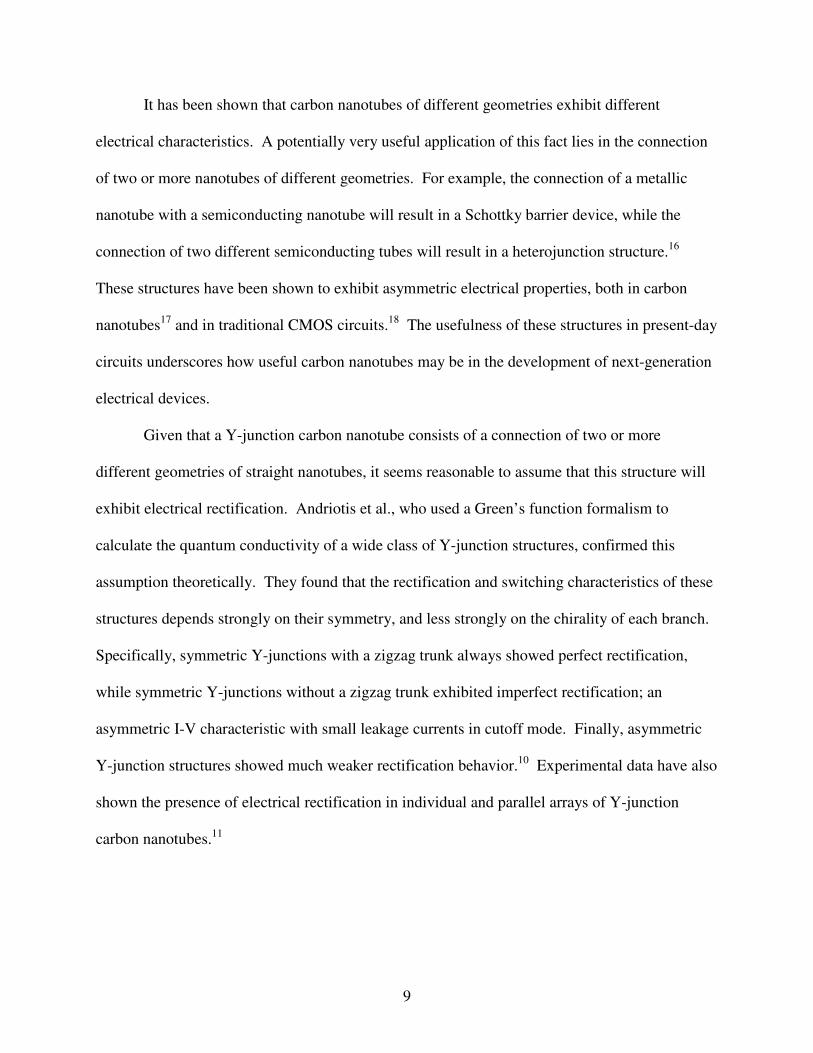
It has been shown that carbon nanotubes of different geometries exhibit different

electrical characteristics. A potentially very useful application of this fact lies in the connection

of two or more nanotubes of different geometries. For example, the connection of a metallic

nanotube with a semiconducting nanotube will result in a Schottky barrier device, while the

connection of two different semiconducting tubes will result in a heterojunction structure.16

These structures have been shown to exhibit asymmetric electrical properties, both in carbon

nanotubes17 and in traditional CMOS circuits.18 The usefulness of these structures in present-day

circuits underscores how useful carbon nanotubes may be in the development of next-generation

electrical devices.

Given that a Y-junction carbon nanotube consists of a connection of two or more

different geometries of straight nanotubes, it seems reasonable to assume that this structure will

exhibit electrical rectification. Andriotis et al., who used a Green’s function formalism to

calculate the quantum conductivity of a wide class of Y-junction structures, confirmed this

assumption theoretically. They found that the rectification and switching characteristics of these

structures depends strongly on their symmetry, and less strongly on the chirality of each branch.

Specifically, symmetric Y-junctions with a zigzag trunk always showed perfect rectification,

while symmetric Y-junctions without a zigzag trunk exhibited imperfect rectification; an

asymmetric I-V characteristic with small leakage currents in cutoff mode. Finally, asymmetric

Y-junction structures showed much weaker rectification behavior.10 Experimental data have also

shown the presence of electrical rectification in individual and parallel arrays of Y-junction

carbon nanotubes.11

10

2.4. Thermal Properties

One of the more interesting aspects of the thermal characteristics of carbon nanotubes is

their thermal conductivity. Thermal conductivity is defined according to

TJ ∇⋅−= κ�

, (2.1)

where J�

is the thermal energy flux, T is the temperature, and � is the thermal conductivity.18

The thermal conductivity gives a measure of how much heat will flow through a solid in

response to a temperature gradient across the solid. When discussing heat flow, it is useful to

identify what exactly is carrying the heat across the temperature gradient. In metals, electrons

are the heat carriers. In crystals such as carbon nanotubes, lattice vibrations known as phonons

carry heat. When heat conduction is thought of in this way, the thermal conductivity can be

written as

Cvl31=κ , (2.2)

where C is the lattice heat capacity, v is the average phonon velocity, and l is the mean free

path of the phonons. Heat capacity is a relationship between a change in temperature of the

crystal and a corresponding change in the number of phonon modes present. The mean free path

describes the average distance a phonon will travel before giving up its energy in some sort of

collision.18

From equation (2.2), it can be seen that the temperature dependence of the thermal

conductivity of a crystal is determined by the temperature dependences of C, v , and l . For the

11

sake of simplicity, v can be treated as independent of temperature. In three dimensions, the

specific heat varies as T3 at low temperatures, and eventually levels off to a constant value at

high temperatures, when all the phonon modes have been excited. At low temperatures, the

mean free path of the phonons is relatively long, and is thus limited by the boundaries of the

crystal. Therefore, at low temperatures the mean free path is more or less constant, and the

thermal conductivity should vary as T3. As the temperature increases, phonons of shorter

wavelengths are excited, and localized defects cause the mean free path to decrease, which

causes the thermal conductivity to fall below the T3 trend. At higher temperatures, the phonons

are energetic enough that the majority of their collisions will result in umklapp scattering, which

reduces the total phonon momentum and increases the thermal resistance. Thus, at high

temperatures the mean free path is the average distance between umklapp collisions. It has been

found that l is proportional to 1/T at high temperatures, meaning that the thermal conductivity is

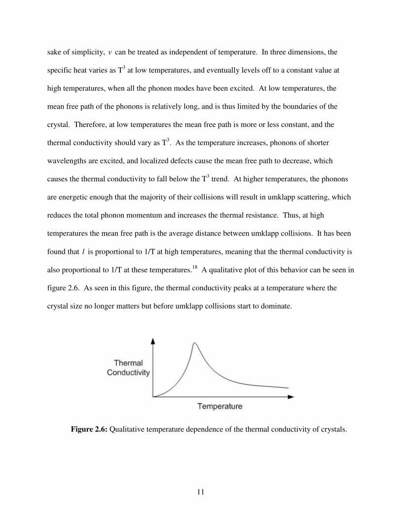
also proportional to 1/T at these temperatures.18 A qualitative plot of this behavior can be seen in

figure 2.6. As seen in this figure, the thermal conductivity peaks at a temperature where the

crystal size no longer matters but before umklapp collisions start to dominate.

Figure 2.6: Qualitative temperature dependence of the thermal conductivity of crystals.

12

A variety of studies have been conducted on the thermal conductivity of carbon

nanotubes. Hone et al. measured the temperature-dependent thermal conductivity of mats of

carbon nanotubes. By comparing these values to the electrical conductivity of individual

nanotubes and mats of nanotubes, they estimated the room temperature thermal conductivity of

an individual nanotube to be in the range 1750-5800 W/m-K.19 Using a combination of

equilibrium and non-equilibrium molecular dynamics simulations, Berber et al. predicted the

room temperature thermal conductivity of a single (10,10) carbon nanotube to be approximately

6600 W/m-K.5 Other molecular dynamics simulations predicted this value to be from 1600

W/m-K to 3000 W/m-K.20,21 While these results show a good deal of variation, they all suggest

that the thermal conductivity of carbon nanotubes is at least as high as those of diamond and

graphite, making them some of the best thermal conductors known. In later measurements, Hone

et al. found that the thermal conductivity of an array of single-wall carbon nanotubes peaked at

around 400 K.22 Measurements on multi-wall carbon nanotubes have shown a thermal

conductivity that peaks at around 300 K.23 This is in contrast to diamond and graphite, whose

thermal conductivities peak at around 150 K.22 This indicates that umklapp scattering occurs at

much higher temperatures in carbon nanotubes than it does in diamond and graphite. As a result,

carbon nanotubes could be significantly better conductors at higher temperatures.

Another interesting thermal property of carbon nanotubes can be seen at very low

temperatures. In 1998, Rego and Kirczenow used the Landauer formulation of transport to

predict a universal quantum of thermal conductance of hTkB

322π in 1D quantum wires at very

low temperatures.24 In 2000, Schwab et al. experimentally confirmed this value of quantized

thermal conductance in silicon nitride nanowires.25 Given these results, a linear temperature

dependence of the thermal conductivity or heat capacity of a material at low temperatures should

13

indicate the presence of quantized thermal conductance. Hone et al. have observed this linear

temperature dependence in the thermal conductivity of single-wall carbon nanotubes at

temperatures below 30 K.19 More recently, Hone and his colleagues observed a linear

temperature dependence of the specific heat capacity of single-wall carbon nanotubes at

temperatures below 8 K.26 Both of these results indicate the presence of quantized thermal

conductance in single-wall carbon nanotubes.

Given their structure, Y-junction nanotubes can be expected to exhibit similar thermal

characteristics to straight carbon nanotubes. However, the presence of the junction in the middle

of the structure suggests that some fundamental differences between their thermal properties

should exist. Up to this point no studies on the thermal properties of Y-junction carbon

nanotubes have been conducted.

14

CHAPTER THREE

MOLECULAR DYNAMICS

3.1. Introduction

Molecular dynamics simulation is a classical approach to modeling systems of atoms and

molecules. It makes use of Newton’s laws of motion and an accurate interatomic potential to

determine the motion of each atom or molecule in the system. With detailed knowledge of the

motion of each particle in the system, a variety of useful information can be determined. In the

sections below, the general approach used in molecular dynamics is discussed, as are some of the

more specific calculations made in the course of this research.

3.2. General Method

As stated above, the molecular dynamics approach is classical in the sense that it makes

use of Newtonian mechanics to determine the behavior of the system. In order to determine the

forces acting on each atom in a particular system, an interatomic potential function is used. The

potential function defines the potential energy between a pair of atoms as a function of their

distance from one another. Thus, the potential function can be written as U(rij), where rij

represents the distance between the ith and jth atoms in the system under investigation. For the

sake of simplicity in notation, this is rewritten as Uij. Once the potential energy between a pair

of atoms is known, the force between the two atoms can be found by taking the gradient of the

potential function with respect to their distance: ijij UF −∇=�

. Then, the net force on a particular

atom can be found by summing the forces due to all other atoms in the system: �≠

∇−=ij

iji UF�

.

15

Once the net force on a particular atom is known, its acceleration at a particular instant in time is

easily derived using Newton’s second law of motion:

iii mFa /�� = (3.1)

In equation (3.1), mi is the mass of the atom in question.27

Above it was stated that the force on a particular atom is determined as a sum of the

forces due to all the other atoms in the system. This is the case because most potential functions

have an infinite range. In practice, however, the large number of atoms in many systems makes

this approach computationally unfeasible. Therefore, it is necessary to limit the number of

contributors to the force on a particular atom. One way to do this is to introduce a cutoff term to

the potential function that limits its effect to a specific range. Thus, any atoms separated by

more than this range would not interact with one another. The potential function used in this

research includes a cutoff term. Another method used in these simulations is the nearest-

neighbor method. The potential function used in this research describes the potential energy

between a pair of bonded carbon atoms. Thus, it should not be applied to a pair of carbon atoms

that are not directly bonded together. A given atom in a carbon nanotube can be bonded with

only its nearest neighbors. Therefore, a list of nearest neighbors for each atom is maintained,

which significantly limits the number of pair-wise interactions that must be calculated.

To account for the movement of the atoms in the system over time, the simulation is

broken into a series of sequential time steps. At each time step the details of the movement of

each atom are calculated. This is usually done using a predictor-corrector scheme. In this

scheme, a Taylor series expansion is used to predict the position, velocity, acceleration, and

16

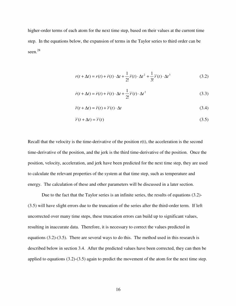
higher-order terms of each atom for the next time step, based on their values at the current time

step. In the equations below, the expansion of terms in the Taylor series to third order can be

seen.28

32 )(!3

1)(

!21

)()()( ttrttrttrtrttr ∆⋅+∆⋅+∆⋅+=∆+ ������ (3.2)

2)(!2

1)()()( ttrttrtrttr ∆⋅+∆⋅+=∆+ ������� (3.3)

ttrtrttr ∆⋅+=∆+ )()()( ������� (3.4)

)()( trttr ������ =∆+ (3.5)

Recall that the velocity is the time-derivative of the position r(t), the acceleration is the second

time-derivative of the position, and the jerk is the third time-derivative of the position. Once the

position, velocity, acceleration, and jerk have been predicted for the next time step, they are used

to calculate the relevant properties of the system at that time step, such as temperature and

energy. The calculation of these and other parameters will be discussed in a later section.

Due to the fact that the Taylor series is an infinite series, the results of equations (3.2)-

(3.5) will have slight errors due to the truncation of the series after the third-order term. If left

uncorrected over many time steps, these truncation errors can build up to significant values,

resulting in inaccurate data. Therefore, it is necessary to correct the values predicted in

equations (3.2)-(3.5). There are several ways to do this. The method used in this research is

described below in section 3.4. After the predicted values have been corrected, they can then be

applied to equations (3.2)-(3.5) again to predict the movement of the atom for the next time step.

17

This process continues until the target number of time steps has been reached. A schematic of

this process can be seen in figure 3.1 below.

Figure 3.1: High-level process of molecular dynamics simulation.

3.3. The Tersoff-Brenner Interatomic Potential

In the section above, the role of the interatomic potential was discussed. Tersoff first

developed the basis for the potential used in this research for the simulation of covalent silicon.29

18

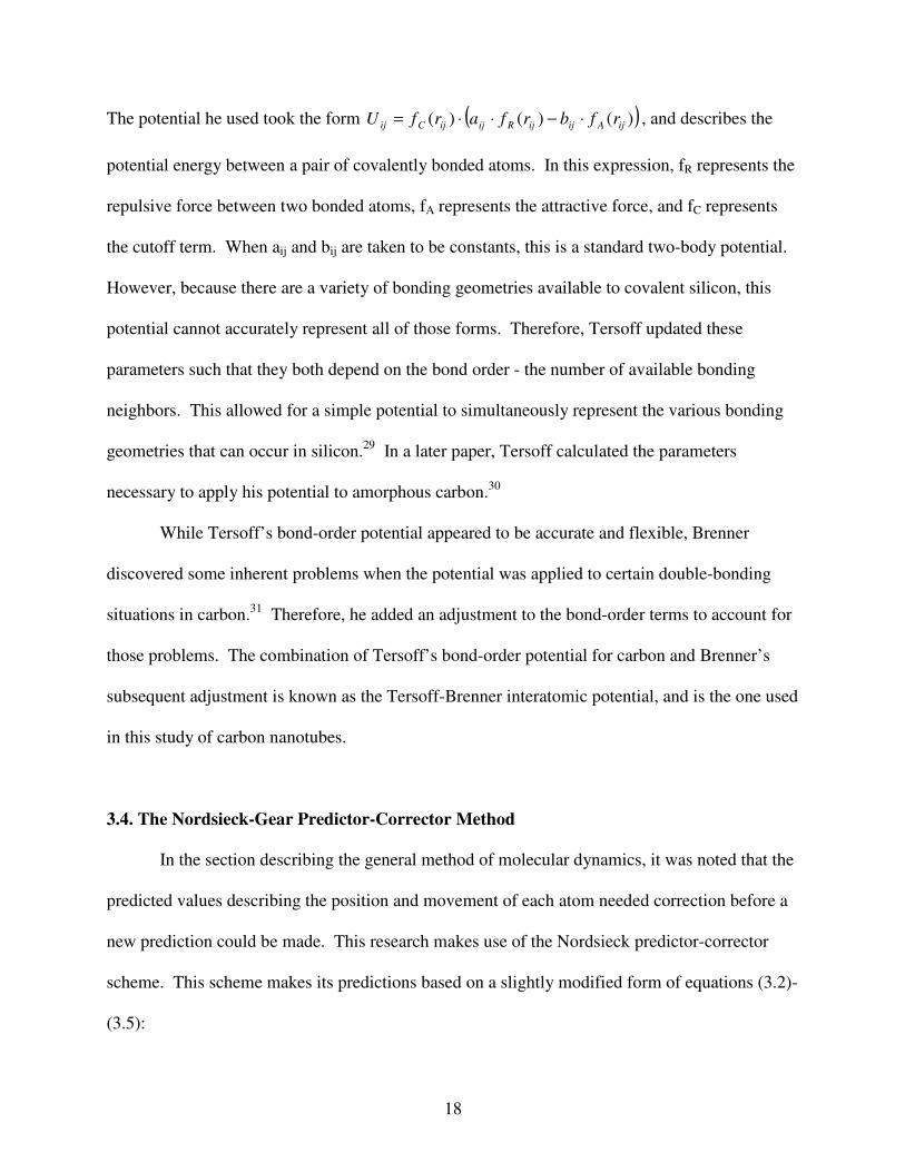
The potential he used took the form ( ))()()( ijAijijRijijCij rfbrfarfU ⋅−⋅⋅= , and describes the

potential energy between a pair of covalently bonded atoms. In this expression, fR represents the

repulsive force between two bonded atoms, fA represents the attractive force, and fC represents

the cutoff term. When aij and bij are taken to be constants, this is a standard two-body potential.

However, because there are a variety of bonding geometries available to covalent silicon, this

potential cannot accurately represent all of those forms. Therefore, Tersoff updated these

parameters such that they both depend on the bond order - the number of available bonding

neighbors. This allowed for a simple potential to simultaneously represent the various bonding

geometries that can occur in silicon.29 In a later paper, Tersoff calculated the parameters

necessary to apply his potential to amorphous carbon.30

While Tersoff’s bond-order potential appeared to be accurate and flexible, Brenner

discovered some inherent problems when the potential was applied to certain double-bonding

situations in carbon.31 Therefore, he added an adjustment to the bond-order terms to account for

those problems. The combination of Tersoff’s bond-order potential for carbon and Brenner’s

subsequent adjustment is known as the Tersoff-Brenner interatomic potential, and is the one used

in this study of carbon nanotubes.

3.4. The Nordsieck-Gear Predictor-Corrector Method

In the section describing the general method of molecular dynamics, it was noted that the

predicted values describing the position and movement of each atom needed correction before a

new prediction could be made. This research makes use of the Nordsieck predictor-corrector

scheme. This scheme makes its predictions based on a slightly modified form of equations (3.2)-

(3.5):

19

32 )(!3

1)(

!21

)()()( ttrttrttrtrttr ∆⋅+∆⋅+∆⋅+=∆+ ������ (3.6)

32 )(!2

1)()()()( ttrttrttrtttr ∆⋅+∆⋅+∆⋅=∆⋅∆+ ������� (3.7)

!2)(

)(!2)(

)(!2)(

)(322 t

trt

trt

ttr∆⋅+∆⋅=∆⋅∆+ ������� (3.8)

!3)(

)(!3)(

)(33 t

trt

ttr∆⋅=∆⋅∆+ ������ (3.9)

Then, the vector z(t) and the matrix A are defined such that

������

�

�

������

�

�

∆⋅

∆⋅

∆⋅

=

!3)(

)(

!2)(

)(

)()(

)(

3

2

ttr

ttr

ttr

tr

tz

���

��

�

and

����

�

�

����

�

�

=

1000310032101111

A . (3.10)

Thus, the prediction consists of the matrix equation )()( tzAttz P ⋅=∆+ .28 The superscript P

indicates that the values are the predicted values.

For correction, the Nordsieck formulation makes a comparison between the acceleration

calculated in equation (3.4), )( ttr ∆+�� , and that calculated from the interatomic potential in

equation (3.1), )( tta ∆+ . Then, the error can be defined as [ ]!2)(

)()()(2t

ttrttate∆∆+−∆+= �� .

To correct this error, the results of equations (3.6)-(3.9) are scaled by a value proportional to the

error in the acceleration, such that28

����

�

�

����

�

�

⋅+∆+=∆+

3/11

6/56/1

)()()( tettzttz P . (3.11)

20

3.5. Calculation of System Properties

This section details the calculation of the various system properties used in this research

on Y-junction carbon nanotubes.

3.5.1. Kinetic Energy

Because the velocity of each atom is known at every time step, the total kinetic energy of

a group of N atoms at a specific point in time is just the sum of their individual kinetic energies:

�=

=N

iiigroup vmE

1

2

21

. The average kinetic energy per atom is obtained by dividing by the total

number of atoms in the group: �=

=N

iiiavg vm

NE

1

2

211

.

3.5.2. Temperature

According to the law of equipartition,32 temperature is proportional to the average atomic

kinetic energy. In three dimensions TkE Bavg 23= , where kB is Boltzmann’s constant. Thus,

using the calculation of average energy in section 3.5.1, the temperature of a group of atoms is

B

avg

k

ET

3

2= .

It should be noted that this definition of temperature applies to the high temperature

regime, where quantum effects are not important. At lower temperatures, this definition is not

necessarily accurate. However, Che et al. have argued that the classical heat flux autocorrelation

can successfully replace its quantum counterpart, even in the low temperature range.21 It is

possible that this argument can be extended to the definition of temperature at low temperatures.

21

3.5.3. Velocity Autocorrelation Function

As discussed in section 3.2, molecular dynamics simulations give the position, velocity,

and acceleration of the atoms in a given system over time. Thus it is possible to use molecular

dynamics to study the time evolution of a system. Time correlation functions provide a way to

do this. To develop the concept of a time correlation function, let p(t) and q(t) denote all the

momenta and spatial coordinates of the system in question. Next, define a pair of variables A

and B that are dependent on p(t) and q(t). Then, it is possible to say that

( ) ( ) ( )tAtqpAtqtpA == );0(),0()(),( and ( ) ( ) ( )tBtqpBtqtpB == );0(),0()(),( . The time

correlation function of variables A and B is defined as:

),();,()0;,()()0()( qpftqpBqpAdpdqtBAtCAB ��== . (3.12)

In equation (3.12), f(p,q) represents the equilibrium distribution of p and q. When

variables A and B are equal, this function is referred to as an autocorrelation function. When the

variables are vector-valued quantities, a dot product is used in equation (3.12). For example, the

velocity autocorrelation function described below is written as )()0()( tvvtCvv�� ⋅= . Another

important feature of this function is that taking its Fourier transform can reveal important

frequency-dependent information about the variables used in the function.33

Equation (3.12) can very difficult to calculate analytically. In the case of the velocity

autocorrelation function, Cvv(t), the dependence of the velocities on position and momentum can

be very complicated, and will involve some form of equations (3.2)-(3.5) as well as the

interatomic potential. Fortunately, an analytical solution is not required when working with

molecular dynamics. Since the velocities are already known at each time step, the dependence of

22

the velocity on p(t) and q(t) does not need to be considered; it has already been included in the

calculation. Thus, the velocity can be treated solely as a function of time, making the calculation

of Cvv(t) fairly straightforward.

Using the argument in the previous paragraph, the velocity autocorrelation function can

be written )()0()( kkvv tvvtC �� ⋅= . The subscript k has been included because of the quantization

of time into discrete steps. This expression refers to the autocorrelation function of the velocity

of a single atom. However, it is useful to consider the average motion of a group of atoms in a

system. In addition, the autocorrelation function does not need to start at time zero. Rather, it

can start at any reference time during the course of the simulation. Therefore, the velocity

autocorrelation function can be updated to �=

+⋅=M

ikiikvv tvv

MtC

1

)()(1

)( ττ �� , where M is the

number of atoms under investigation and � is the reference time. Another convention that is

usually taken in molecular dynamics simulations is to normalize the velocity autocorrelation

function with respect to its initial value:

�

�

=

=

⋅

+⋅==

M

iii

M

ikii

vv

kvvkvv

vvM

tvvM

CtC

tC

1

1

)()(1

)()(1

)0()(

)(~

ττ

ττ

��

��

. (3.13)

Finally, during the course of a simulation it is possible to calculate several normalized

velocity autocorrelation functions concurrently, with each starting at a different reference time.

These separate functions are then averaged together to obtain an overall result. Denoting a

23

particular autocorrelation function with starting time �j as )(~

kj

vv tC , the overall velocity

autocorrelation function can be written as

��

��

=

=

=

= ⋅

+⋅==

N

jM

ijiji

M

ikjijiN

jk

jvvkvv

vv

tvv

NtC

NtC

1

1

1

1 )()(

)()(1

)(~1

)(~

ττ

ττ

��

��

. (3.14)

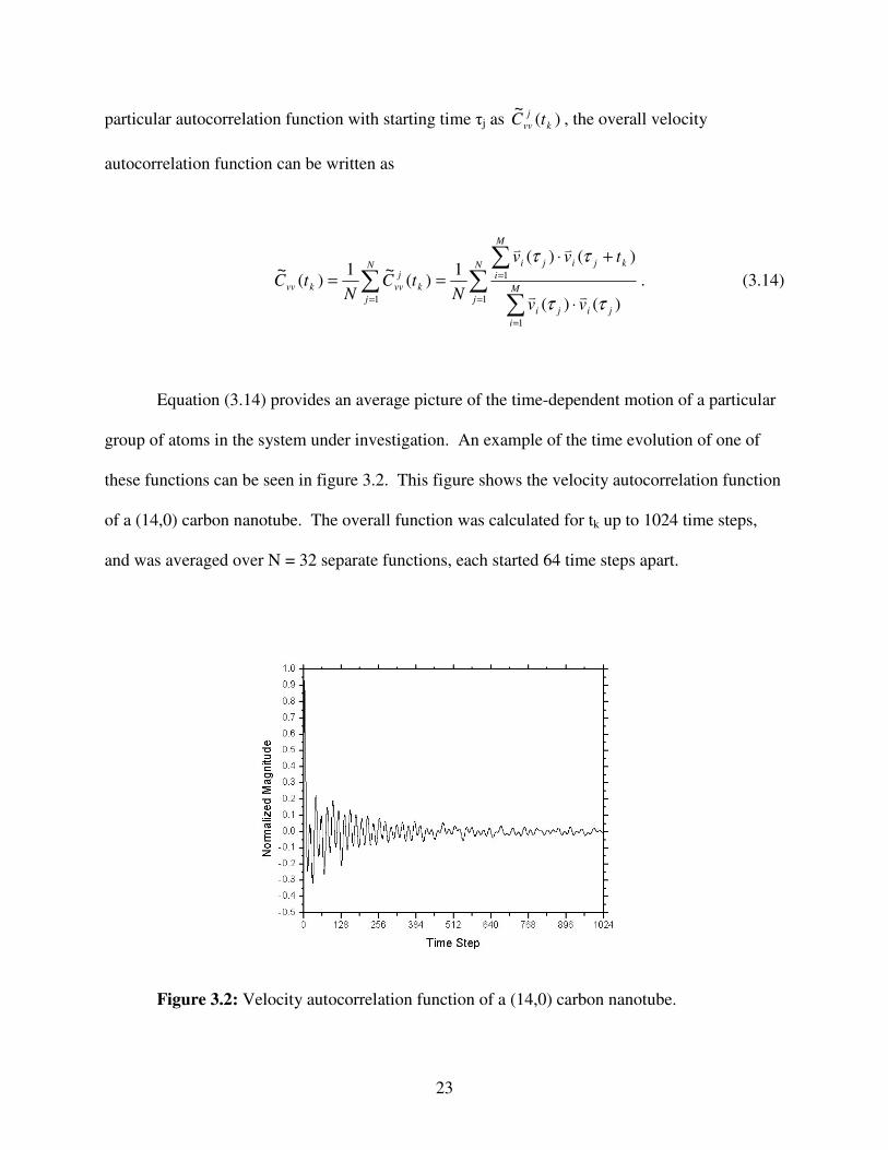
Equation (3.14) provides an average picture of the time-dependent motion of a particular

group of atoms in the system under investigation. An example of the time evolution of one of

these functions can be seen in figure 3.2. This figure shows the velocity autocorrelation function

of a (14,0) carbon nanotube. The overall function was calculated for tk up to 1024 time steps,

and was averaged over N = 32 separate functions, each started 64 time steps apart.

Figure 3.2: Velocity autocorrelation function of a (14,0) carbon nanotube.

24

As stated above, the Fourier transform of time correlation functions can reveal important

information about the variables included in the function. In the case of the velocity

autocorrelation function, the Fourier transform represents the spectral density of the atomic

motions, and can be used to determine which modes of vibration are dominant in a given system.

Some examples of this analysis can be found in Chapter 4.

3.5.4. Thermal Conductivity

Several approaches to calculating the thermal conductivity of a system using molecular

dynamics simulations have been proposed.34-36 The details of the approach used in this research

can be found in Chapter 4, which discusses the thermal properties of Y-junction carbon

nanotubes under steady state conditions.

25

CHAPTER FOUR

STEADY STATE HEAT FLOW

4.1. Introduction

As stated in Chapter 2, up to this point no studies have been conducted on the thermal

properties of Y-junction carbon nanotubes. In this chapter, a molecular dynamics approach to

the modeling of steady state heat flow in a Y-junction carbon nanotube is presented. The goal is

to calculate the thermal conductivity of the Y-junction structure, and determine how it might

differ from that of a straight carbon nanotube. In the following sections, the method for

determining the thermal conductivity is described, the results are presented, and an analysis of

these results is provided.

4.2. Methodology

To model the dynamics of the atoms within the Y-junction nanotube, a molecular

dynamics approach has been chosen, with the Tersoff-Brenner bond order potential for the C-C

bond as the potential interaction function.30,31 Within the molecular dynamics paradigm, a

variety of approaches to the calculation of thermal conductivity have been examined.34-36 The

approach discussed by Oligschleger and Schön,34 and implemented in straight carbon nanotubes

by Osman and Srivastava,20 splits the nanotube into a series of equal “slabs” of atoms. Two of

the slabs are thermally regulated to enforce a temperature gradient upon the system, as shown in

figure 4.1.

26

Figure 4.1: Molecular dynamics setup for calculating the thermal conductivity of a straight carbon nanotube. The ellipses indicate that periodic boundary conditions are applied.

The temperature of each of these slabs is regulated by a scaling of the velocities of the

atoms within the slab. The velocities are scaled according to

current

controloldinewi T

Tvv ⋅= ,, , (4.1)

where Tcontrol is the desired temperature of the slab, and Tcurrent is the current slab temperature. In

this approach, Tcontrol = Tamb+ ∆ T for the hot slab and Tcontrol = Tamb- ∆ T for the cold slab, where

Tamb is the initial temperature of the solid. The change in energy of the controlled slabs at each

time step is given by

( )�=

−=∆N

ioldinewislab vvmE

1

2,

2,2

1, (4.2)

where N is the number of atoms in the slab, m is the mass of each atom, and vi,new is calculated

according to equation (4.1). The heat flux density at the nth time step of the simulation is

calculated by taking an average of the net energy added at each previous time step:

27

tn

jEjE

AnJ

n

jcoldslabhotslab

∆⋅

∆+∆⋅=�

=1

)()(1

)( , (4.3)

where the )( jEslab∆ come from equation (4.2), ∆ t is the time associated with each simulation

step, and A is the cross-sectional annular ring area of the nanotube.20 After a large number of

simulation steps, an equilibrium value of the heat flux density is obtained. The temperature

gradient, dT/dz, is found by applying a linear fit to the temperatures of the slabs in the gray

region in figure 4.1, and the thermal conductivity at the nth simulation step is the quotient of the

heat flux density and the temperature gradient:

dzdTnJ

n/

)()( =κ , (4.4)

where J(n) is given by equation (4.3). One final note that should be made from figure 4.1 is that

periodic boundary conditions have been applied in order to eliminate edge effects.34

To investigate the thermal conductivity of the Y-junction nanotube, an algorithm similar

to that described by Oligschleger and Schön has been chosen. The setup is similar to that shown

in figure 4.1, except for the fact that, due to its linear asymmetry, periodic boundary conditions

cannot be applied to the Y-junction configuration. Therefore, an alternate setup has been chosen,

and can be seen in figure 4.2. In this setup, the black slabs labeled “Fixed” have atoms that are

fixed in space in order to prevent tube drift and oscillations during the simulation. The slabs

labeled “Hot” and “Cold” are the velocity-scaled slabs, whose temperatures are controlled as

described in equation (4.1). The energy flux density at the nth simulation step is calculated in the

28

Figure 4.2: Molecular dynamics setup for calculating the thermal conductivity of the Y-junction nanotube.

same manner as in equation (4.3), but with an extra term to account for the fact that there are two

cold velocity-scaled slabs instead of just one:

tn

jEjEjE

AnJ

n

jcoldcoldhot

∆⋅

∆+∆+∆⋅=�

=121 )()()(

1)( . (4.5)

The slabs labeled “Buffer” act as thermal reservoirs, in an attempt to minimize edge

effects by providing a buffer between the velocity-scaled slabs and the fixed tube ends. The

temperature of these buffer slabs is the same as that of their adjacent velocity-scaled slabs.

However, their temperature is maintained through a more realistic application of friction and

random forces, which satisfy the fluctuation-dissipation theorem through the Langevin dynamics

approach. In order to obtain a single temperature gradient dT/dx for the entire structure, the

positions and temperatures of corresponding slabs in the two branches were averaged before a

linear fit was calculated.

In the algorithm described above, a temperature gradient is imposed by a set of thermal

reservoirs and the resultant heat flux is measured to determine the thermal conductivity of the Y-

junction nanotube. Müller-Plathe has proposed carrying out this process in the reverse order. In

29

his scheme, the velocity of the hottest (most energetic) atom in the cold slab is exchanged with

the velocity of the coldest atom in the hot slab at regular intervals. This has the effect of

imposing a known heat flux on the system. Once a steady state has been reached, the resulting

temperature gradient is measured to determine the thermal conductivity.35

The velocity-exchange approach has a couple advantages. First, because the temperature

gradient is a quantity that converges much more quickly than heat flux, this method requires

much fewer time steps than the thermal reservoir method used in this research. Second, the

resultant temperature gradient tends to be smaller than in the thermal reservoir approach.

Because the thermal conductivity of a material is normally temperature-dependent, a large

temperature gradient can result in a large variation in the local thermal conductivity across the

system. A small temperature gradient allows a more accurate measure of the system’s overall

thermal conductivity.35 However, the application of this method in the Y-junction structure is

problematic because of the presence of two cold reservoirs and only one hot reservoir. It would

be difficult to ensure that the two branches are maintained at the same temperature.

Another approach makes use of a fictitious force field applied along the direction of heat

flow. This fictitious field imposes a heat flux on the system under investigation by forcing hot

and cold atoms in opposite directions. This approach has the advantage of inducing no

temperature gradient, and as the fictitious field gets small, a very accurate value of thermal

conductivity can be obtained. However, this method relies on the assumption of periodic

boundary conditions, which cannot be applied to the Y-junction structure.

As stated earlier, the linear asymmetry of the Y-junction structure precludes the

application of periodic boundary conditions to the system. The buffer slabs were added in an

attempt to provide a shield from edge effects, but it is still possible that the tube ends could have

30

an effect on the heat flow within the system. Furthermore, the alternate methods described

above may provide more accuracy than the method chosen. Thus, absolute magnitude of the

thermal conductivity may not be as accurate as it could be. The chosen method, however, is

reasonable for identifying trends and relative magnitudes of heat transport in a branched

nanotube structure in comparison with straight nanotubes with or without defects.

4.3. Results

For the molecular dynamics simulations, a Y-junction with a (14,0) zigzag trunk splitting

into two (7,0) zigzag branches was used. There were 35 slabs in each of the three branches, and

one slab in the middle connecting them, for a total of 106 slabs including 3980 atoms. With a

length of 4.26 Å per slab, each branch in the tube measured about 15 nm long. This is long

enough for a qualitative comparison of thermal transport in branched and straight carbon

nanotubes, but not for absolute values of thermal conductivity. The thermal conductivity

simulation was run at base temperatures of 200 K to 400 K in increments of 50 K. A

temperature differential of ± 50 K between the trunk and the two branches was used in each

case. Two simulations were run for each base temperature, one with a hot trunk and cold

branches (designated as “forward” heat flow), and one with a cold trunk and hot branches

(“reverse” heat flow). For comparison, a (14,0) straight nanotube of 71-slab length was also run

at these temperatures. The straight tube was configured in a manner similar to that shown in

figure 4.2, with the fixed ends, buffer slabs and velocity-scaled slabs. Each simulation was run

for 200,000 time steps, with the heat flux density averaged over the last 100,000 time steps. For

these simulations, the time step was 0.5 fs, and the cross-sectional area was calculated based on

an annular ring width of 3.4 Å.20

31

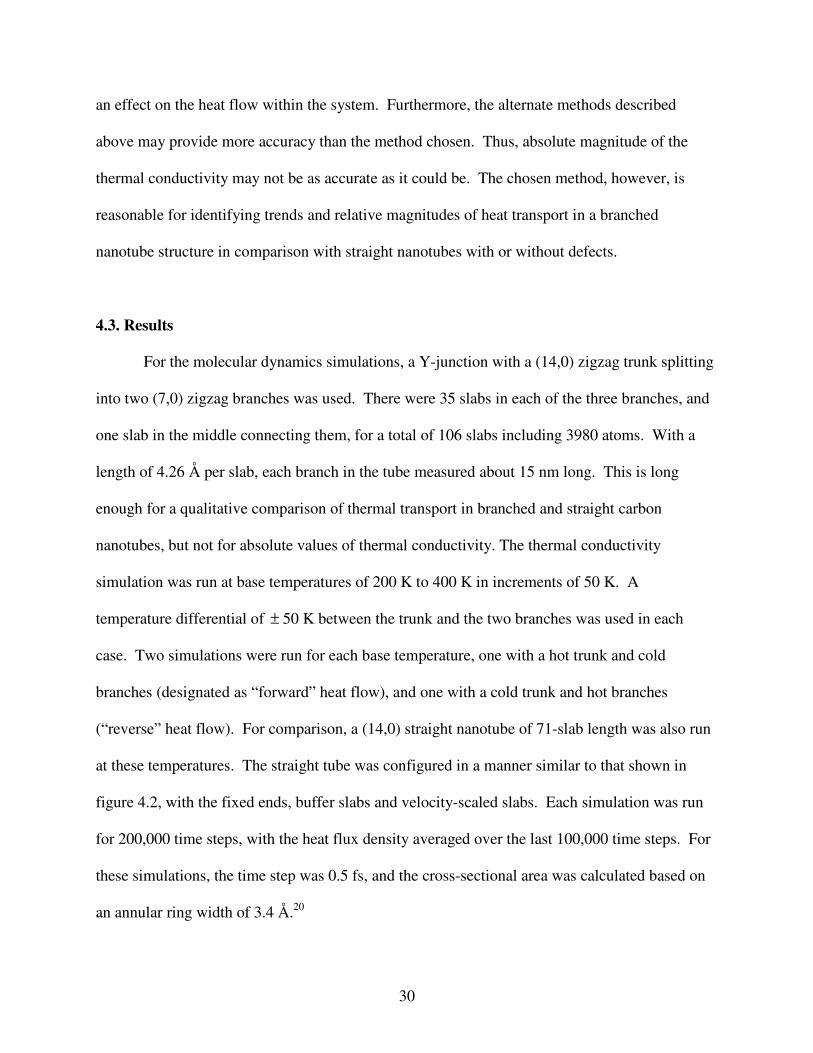
Figure 4.3: Temperature dependence of the thermal conductivity. The squares represent the straight (14,0) nanotube, the triangles represent the forward heat flow configuration of the y-junction tube, and the circles represent the reverse heat flow configuration of the y-junction tube.

The results for the thermal conductivity of the nanotubes are summarized in figure 4.3.

For temperatures up to 400 K, there is no significant difference between the “forward” and

“reverse” heat conductivity of the Y-junction carbon nanotube. This is in contrast to the

theoretical result indicating significant electrical rectification in the same Y-junction nanotube

configuration.10 Additionally, the thermal conductivity exhibits an increase with temperature

similar to what has been reported experimentally19 for straight carbon nanotubes. Figure 4.3 also

indicates that the thermal conductivity of the straight (14,0) nanotube was consistently larger

than that of the Y-junction structure.

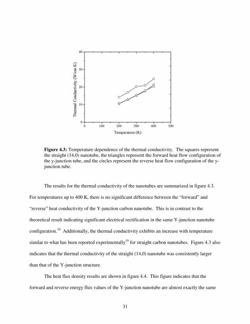
The heat flux density results are shown in figure 4.4. This figure indicates that the

forward and reverse energy flux values of the Y-junction nanotube are almost exactly the same

32

Figure 4.4: Temperature dependence of the heat flux density. The squares represent the straight (14,0) nanotube, the triangles represent the forward heat flow configuration of the y-junction tube, and the circles represent the reverse heat flow configuration of the y-junction tube.

for all temperatures. Furthermore, these flux values are essentially identical to those of the

straight (14,0) nanotube. Given this, it stands to reason that the differences in thermal

conductivity between the Y-junction and the straight nanotubes are due to differences in the

temperature gradient. Figure 4.5 shows the values of the temperature gradient obtained, and

indicates that the Y-junction tube has a higher temperature gradient than the straight (14,0) tube

for all temperatures.

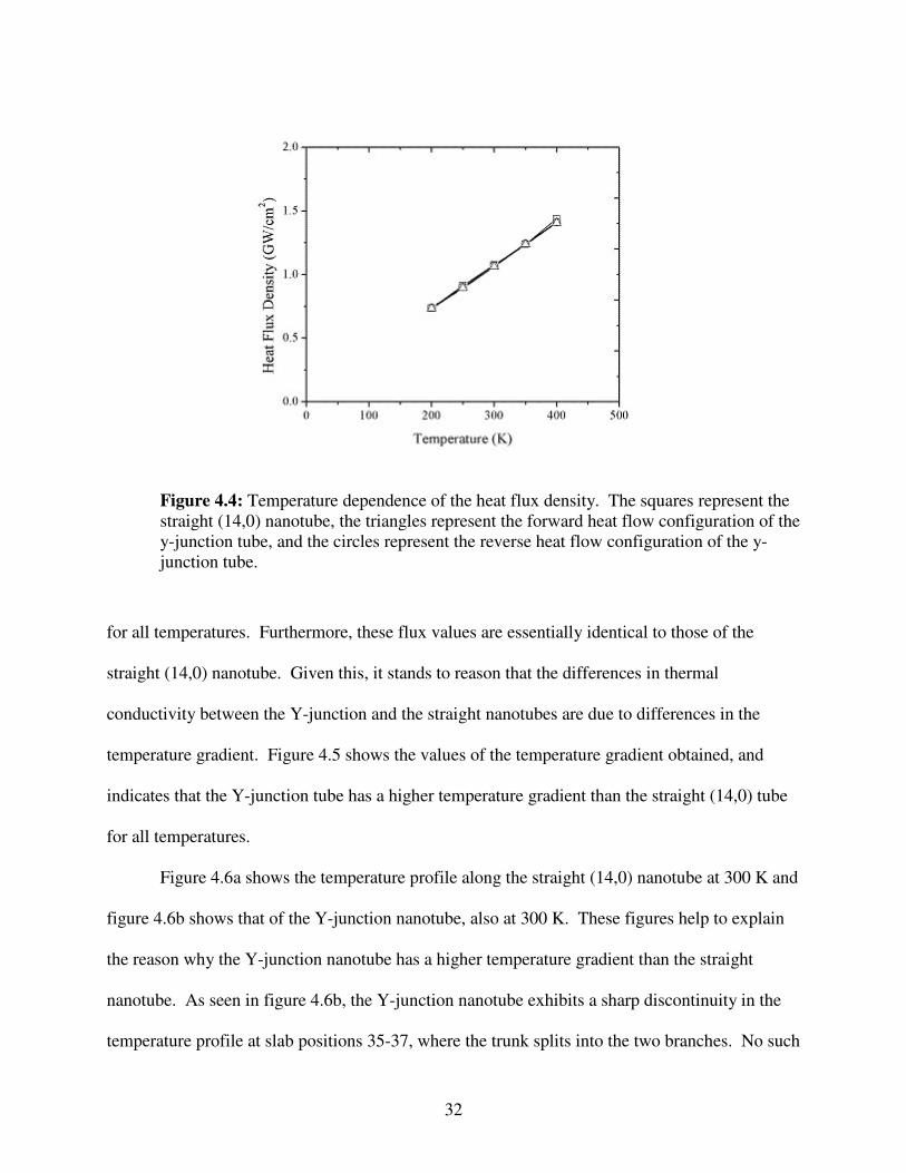
Figure 4.6a shows the temperature profile along the straight (14,0) nanotube at 300 K and

figure 4.6b shows that of the Y-junction nanotube, also at 300 K. These figures help to explain

the reason why the Y-junction nanotube has a higher temperature gradient than the straight

nanotube. As seen in figure 4.6b, the Y-junction nanotube exhibits a sharp discontinuity in the

temperature profile at slab positions 35-37, where the trunk splits into the two branches. No such

33

Figure 4.5: Temperature dependence of the temperature gradient. The squares represent the straight (14,0) nanotube, the triangles represent the forward heat flow configuration of the y-junction tube, and the circles represent the reverse heat flow configuration of the y-junction tube.

discontinuity in the temperature profile exists for the straight tube. This small region of

relatively large temperature gradient is a result of the presence of high resistance to heat flow at

the junction. This high resistance, in turn, results in the lower values for the thermal

conductivity of the Y-junction nanotube.

Discontinuities in the temperature profile have been observed in the context of molecular

dynamics simulations before. Using a non-equilibrium molecular dynamics approach, Maiti et

al. have investigated the heat flow across crystal grain boundaries. They have reported a similar

temperature profile across a grain boundary in a silicon crystal.37 Maruyama et al. have reported

seeing a jump in the temperature profile of a carbon nanotube heterojunction consisting of a

(12,0) tube connected to a (6,6) tube.38 In each of these cases, the jump in the temperature

profile seems to be associated with the presence of discontinuities or defects in the crystal lattice

34

Figure 4.6: Temperature profiles of (a) the straight (14,0) nanotube, (b) the Y-junction nanotube, (c) the straight (14,0) nanotube with vacancy defects, and (d) the straight (14,0) nanotube with a Stone-Wales (5,7,7,5) defect. Fit lines have been added to show the slope in each region.

35

under investigation. These defects act as additional scattering centers and result in a region of

large temperature gradient, which translates to a reduction in the thermal conductivity of the

crystal. Che et al. have reported his type of behavior, with theoretical calculations that indicate

an inverse relationship between the number of defects in a crystal and the thermal conductivity

of the crystal.21 In the Y-junction tube examined in this paper, lattice defects are present in the

form of six heptagonal carbon rings at the junction point.10

In order to understand the origin of the discontinuity at the Y-junction, two types of

defects were intentionally introduced into the middle of two straight (14,0) nanotubes. The first

type of defect was in the form of atomic vacancies and was created by the removal of two atoms

from the middle slab of the tube. The second type of defect was a Stone-Wales (5, 7, 7, 5)

defect, where four hexagons are changed into two pentagons and two heptagons. These tubes

were then run through the simulation at 300 K, with the usual ± 50 K hot and cold slabs applied.

The resulting temperature gradient of the tube with vacancies can be seen in figure 4.6c, while

that of the tube with the Stone-Wales defect can be seen in figure 4.6d. As seen in these figures,

the temperature profile of the straight nanotube with two vacancies is very similar to that of the

Y-junction, while the temperature profile of the tube with the Stone-Wales defect exhibits a

discontinuity that is much less pronounced. Additionally, the resulting values of the temperature

gradient and the thermal conductivity of the (14,0) tubes with defects were calculated. The

nanotube with vacancies had the same thermal conductivity and temperature gradient as those

obtained for the Y-junction nanotube at the same temperature. The nanotube with the Stone-

Wales defect had a smaller temperature gradient and thus a larger thermal conductivity than the

Y-junction tube, but a smaller thermal conductivity than the defect-free (14,0) tube. Che et al.

noted that Stone-Wales defects have a less significant effect on thermal conductivity than

36

vacancies,21 which is consistent with the smaller temperature profile discontinuity seen in figure

4.6d. They concluded that the Stone-Wales defects were less severe because they do not change

the bonding configuration of the lattice and thus induce less structural deformation. The greater

amount of structural deformation in the Y-junction nanotube suggests that it will exhibit a more

significant discontinuity in the temperature profile.

In an attempt to clarify the reason behind the presence of the jump in the temperature

profiles, the phonon spectra of the nanotubes in question were investigated. The phonon spectra

were found by taking the Fourier transform of the velocity autocorrelation functions of each

tube, which were calculated over 1024 time steps in the molecular dynamics simulations. Of

interest were the frequency distributions of atomic vibrations along two different directions.

Axial phonons and radial phonons represent vibrations parallel and perpendicular to the nanotube

axis, respectively. Therefore, two autocorrelation functions were calculated, one using only the

component of the atomic velocities parallel to the nanotube axis, and one using only velocity

components perpendicular to the nanotube axis.

Figure 4.7a shows the axial phonon spectrum of the atoms in a single defect-free slab in

the (14,0) nanotube. A primary peak exists at around 50 THz, with a lesser peak at about 20

THz. In figure 4.7b, the axial phonon spectrum of the atoms in the slab with vacancies in the

(14,0) tube is shown. Again, the phonon density peaks at about 20 THz and 50 THz. However,

the magnitude of the 50 THz peak is about 15% smaller than that of the defect-free slab. Figure

4.7c shows the axial phonon spectrum of the atoms in the slab with the Stone-Wales defect. The

magnitude of the 50 THz peak is about 16% smaller than that of the defect-free slab. Finally,

figure 4.7d shows the axial phonon spectrum of the atoms of slab 35 in the Y-junction tube. Slab

35 is the slab in the (14,0) trunk of the Y-junction that is adjacent to the middle “hub” slab.

37

Figure 4.7: Axial phonon spectra of (a) the straight (14,0) nanotube, (b) the straight (14,0) tube slab with vacancy defects, (c) the straight (14,0) nanotube slab with a Stone-Wales (5,7,7,5) defect, and (d) Y-junction slab 35. These spectra represent atomic vibrations parallel to the tube axis.

Moving from left to right along the temperature profile of the Y-junction tube in figure 4.6b, one

can see that slab 35 is where the first significant discontinuity in the temperature drop occurs.

Again, peaks in the phonon density of the atoms in this slab exist at 20 THz and 50 THz. In this

case the magnitude of the 50 THz peak is about 30% smaller than that in the defect-free (14,0)

slab. Similar results were obtained for the radial phonon spectra of the nanotubes. The

magnitudes of the 50 THz peaks in the radial phonon spectra of the Y-junction and (14,0)

38

nanotube with vacancies were both 7% smaller than that of the defect-free (14,0) nanotube, while

the peak in the tube with the Stone-Wales defect was 20% smaller.

4.4. Discussion

The steady state heat flow properties of a Y-junction nanotube consisting of a (14,0)

trunk splitting into two (7,0) branches have been investigated using molecular dynamics

simulations. Thermal transport under steady state does not show any anisotropy with respect to

the direction of the heat flow, which is in contrast to the evidence of electrical rectification in the

same structure. In their calculations, Andriotis et al. accounted for the effects of quantum states

on electrical conduction in Y-junction carbon nanotubes through an application of Green’s

functions.10 Recent experimentation has shown that the specific heat of carbon nanotubes

increases linearly with temperature from 2 K to 8 K, with an increase in the slope above 8 K.26

This behavior implies a quantized 1D phonon spectrum in carbon nanotubes at temperatures

below 8 K. Above 8 K, the number of phonon modes excited becomes large enough to make the

specific heat appear to be continuous with temperature. Therefore, quantum thermal effects are

not seen at the temperatures used in these simulations. Furthermore, the use of Fourier’s

classical law of heat flow in the MD simulations precludes the inclusion of quantum thermal

effects. Fourier’s law provides an aggregate measure of the thermal conductivity by summing

over all of the present phonon modes,39 but in doing so wipes out information about the

contribution of individual phonons to heat flow. It has been demonstrated that the thermal

conduction of carbon nanotubes at any temperature is dominated by phonons.19 Therefore, it is

possible that a more detailed model including a consideration of individual phonon modes may

reveal thermal rectification in Y-junction nanotubes at very low temperatures.

39

The discontinuity in the temperature profile of the Y-junction nanotube seems to be the

result of the discontinuous crystal structure present at the hub of the Y-junction. Similar

temperature profiles have been observed in crystal grain boundaries,37 junctions between

nanotubes of different diameters,38 and in single nanotubes with vacancy defects present. A

study of the phonon modes in the investigated tubes indicates that the presence of defects

reduces the density of axial and radial phonon modes. This connection between the temperature

discontinuity and the atomic vibrations seems to indicate that both the axial and the radial modes

are at least partly responsible for the transfer of heat along a nanotube, and that the interruption

of these modes results in an interruption of heat transfer.

40

CHAPTER FIVE

HEAT PULSE PROPAGATION

5.1. Introduction

In Chapter 4, the details of the simulation of steady state heat flow through a Y-junction

carbon nanotube were provided. In this chapter, the transient heat flow properties of the Y-

junction nanotube are examined. Molecular dynamics simulations are used to generate a heat

pulse in the Y-junction and examine how it propagates through the structure. In this chapter, the

simulation method is described, the results are summarized and an analysis is provided.

5.2. Methodology

The details of the molecular dynamics simulation used in the study of heat pulse

propagation are similar to those presented in Chapter 4. As before, the Tersoff-Brenner bond

order potential has been used. The general simulation method, as described in Chapter 3, is

exactly the same. The difference lies in the application of heat to the system. In the steady state

case, hot and cold thermal reservoirs were placed at opposite ends of the Y-junction to induce

heat flow. The temperatures of these reservoirs were maintained by velocity scaling through

equation (4.1). In the case of transient heat flow, the setup is slightly different, and can be seen

in figure 5.1.

The slabs labeled “Fixed” and those labeled “Buffer” are the same as those described in

Chapter 4. The buffer slabs are maintained at the ambient temperature of the simulation. The

slabs labeled “Pulse” are those to which the heat pulse is applied. The temperature in the “Pulse”

41

slabs is controlled through velocity scaling as in equation (4.1), but instead of being constant,

Tcontrol is time-dependent. This time-dependence can be seen in figure 5.2.

Figure 5.1: Molecular dynamics setup for applying a heat pulse to the Y-junction carbon nanotube.

Figure 5.2: Time-dependent behavior of the applied heat pulse.

From this figure it should be noted that Tamb is the same ambient temperature at which the

buffer slabs are held. Before and after the heat pulse, the temperature of the “Pulse” slabs is

maintained at Tamb in the same manner as the buffer slabs, with one small adjustment. There is

no fixed slab at the end of the tube where the pulse is applied. This is done in order to minimize

42

reflections from that tube end. However, the absence of a fixed slab results in the possibility of

large-scale oscillations on that end of the tube. These oscillations would be greatly magnified by

velocity scaling during the application of the heat pulse. Therefore, at each time step the center-

of-mass velocity of the pulse slabs is calculated and subtracted from the velocity of each atom.

This ensures that the overall momentum of this end of the tube remains zero.

Because this simulation is a transient one, there is no need to calculate properties based

on statistical averages, such as thermal conductivity or the velocity autocorrelation function.

Instead, it is only necessary to collect the temperature profile data at specific time intervals

throughout the simulation. This data provides the time evolution of the temperature at each point

in the Y-junction nanotube. However, the instantaneous temperature data can be noisy in both

time and space. Therefore, two techniques, spatial and temporal averaging, are used to provide a

smoother picture of the time evolution of the temperature. Spatial averaging determines the local

temperature of each slab by finding the average temperature of the current slab and its two

nearest neighbor slabs on each side. For example, the local temperature of slab 10 is the average

temperature of slabs 8, 9, 10, 11, and 12. In temporal averaging, the temperature of a slab at the

current time step is equal to the average of the temperature of that slab over the previous N time

steps.

5.3. Results

The Y-junction used in these simulations had a (14,0) trunk and two (7,0) branches. Each

branch contained 150 slabs, for a total of 451 slabs and 16,860 atoms. With a slab-width of 4.26

Å, each branch measured about 64 nm long. This is long enough to examine the propagation of

heat pulses through the branches before they reach the junction. The Y-junction nanotube was

43

simulated under three different heat pulse configurations: a heat pulse originating in the (14,0)

trunk, a heat pulse originating in one of the (7,0) branches, and a heat pulse originating in both of

the (7,0) branches simultaneously. Each simulation was run for 30,000 time steps. At 0.5 fs per

step, this is a total time of 15 ps. For comparison, a straight (14,0) nanotube and a straight (7,0)

nanotube each measuring 300 slabs (128 nm) were also run under the heat pulse simulations.

Temporal averaging was taken over an interval of 50 time steps. In each case, the tube in

question was quenched to Tamb = 0 K, while the pulse magnitude was Tpulse = 800 K. The rise

and fall times were trise = tfall = 100 steps (50 fs), the start time was tstart = 1 time step, and the

pulse length was tpulse = 2000 time steps (1 ps).

Figure 5.3 shows the results of the heat pulse simulation on the (7,0) carbon nanotube.

As seen in this figure, the heat pulse has excited several traveling waves. Three of them are of

particular interest in this discussion, and are labeled in figure 5.3. The wave labeled “1” is the

leading edge wave, and travels at a speed of 21.3 km/sec. This speed is consistent with the

sound velocity of longitudinal acoustic phonons in (10,10) armchair nanotubes, which are

estimated to be 20.35 km/sec, and that of 21.0 km/sec in 3D graphite.40 The magnitude of this

leading wave is very small, on the order of 3 K. The second wave of interest, labeled “2,” travels

at approximately 12.8 km/sec, which is similar to the sound velocity of the transverse acoustic

mode in 3D graphite at 12.3 km/sec. The velocities of the transverse acoustic mode of a (10,10)

nanotube and 2D graphite are estimated to be 9.4 km/sec and 15.0 km/sec, respectively, and the

velocity of the twisting mode of a (10,10) nanotube is approximately 15.0 km/sec.40 The

magnitude of this wave is relatively large, on the order of 130 K. The final mode of interest,

labeled “3,” travels at 6.4 km/sec and precedes diffusive heat flow in the (7,0) nanotube, due to

increase in overall temperature behind it. The leading wave in the diffusive heat flow has a

44

Figure 5.3: Heat pulse results of the (7,0) carbon nanotube.

magnitude on the order of 25 K. Henceforth, these waves will be known as type-1, type-2 and

type-3 waves, corresponding to their labels in figure 5.3. The waves seen in subsequent figures

will also be labeled accordingly.

45

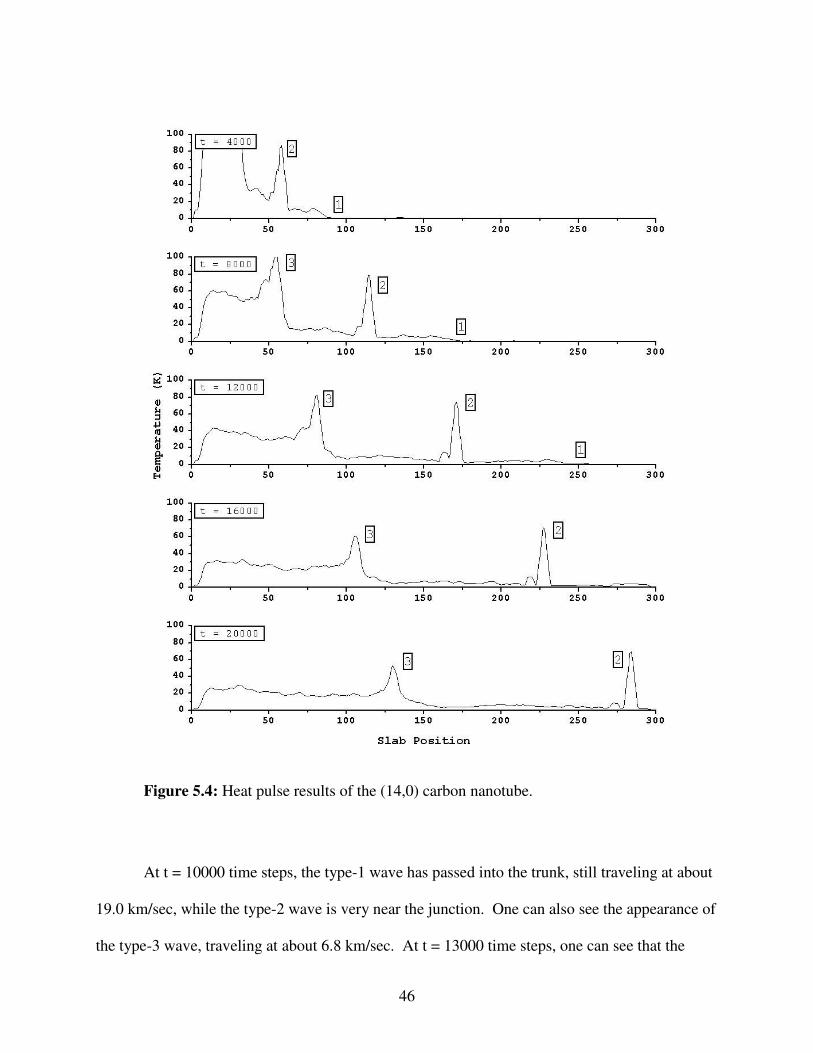
Figure 5.4 shows the results of the heat pulse simulation on the (14,0) carbon nanotube.

The labeled waves correspond to those in figure 5.3. The type-1 leading edge wave of the (14,0)

nanotube travels at a velocity of 18.3 km/sec, and has a magnitude on the order of 0.5 K. The

type-2 wave travels at approximately 12.1 km/sec, with a magnitude of about 70 K. The type-3

wave travels at 5.5 km/sec with a maximum pulse magnitude of around 50 K. From these results

it can be seen that these waves propagate slightly slower in the (14,0) nanotube than they do in

the (7,0) nanotube. One other thing to note is that the type-2 wave appears to have a second peak

trailing along behind it at the same velocity. This could be the result of a reflection of this wave

off the tube end, which would explain its reduced magnitude. It is unclear why this is not

observed in the (7,0) nanotube.

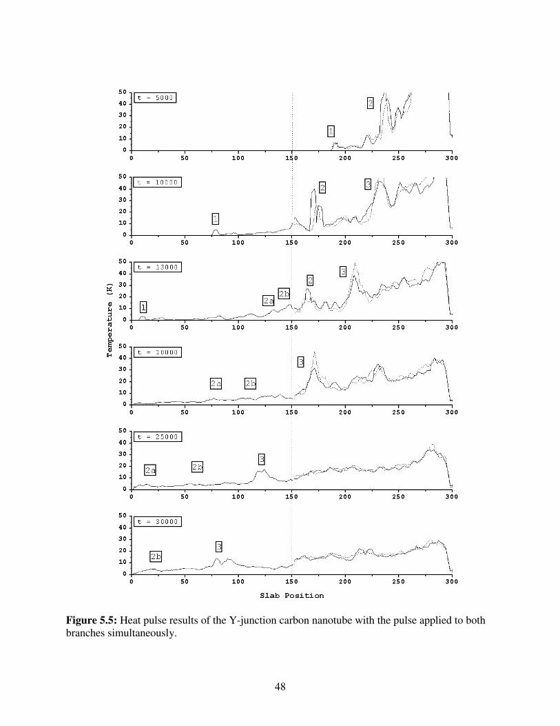
Figure 5.5 shows the results when the heat pulse is applied to both branches

simultaneously. In this figure, slabs 1-150 represent the (14,0) trunk region. The solid curve

along slabs 152-301 represents the first (7,0) branch, while the broken curve represents the

second one. Slab 151 is the hub of the Y-junction structure. The vertical broken line at slab 150

is used to indicate the location of the junction. In this figure, it can be seen that some of the

waves that reach the junction are transmitted into the (14,0) trunk, but with a reduced magnitude.

The waves of interest in this figure have been labeled corresponding to their type. At t = 5000

time steps, one can see that type-1 and type-2 waves are propagating in the branches toward the

junction at about 19.0 km/sec and 10.6 km/sec, respectively. It appears that the magnitude of the

type-2 wave in branch 2 is larger than that in branch 1. This could be due to a variation in the

initial noise conditions of the branches. The tube was quenched at a low temperature for a long

time, but perhaps only a slight difference in noise conditions can result in a magnitude difference

of this scale.

46

Figure 5.4: Heat pulse results of the (14,0) carbon nanotube.

At t = 10000 time steps, the type-1 wave has passed into the trunk, still traveling at about

19.0 km/sec, while the type-2 wave is very near the junction. One can also see the appearance of

the type-3 wave, traveling at about 6.8 km/sec. At t = 13000 time steps, one can see that the

47

type-2 waves in the branches have collided with the junction, and have partially reflected back

into the branches. As a result, two waves have been generated in the trunk, one traveling at a

velocity of 9.5 km/sec and the other traveling at a velocity of 6.4 km/sec. These waves have

been labeled “2a” and “2b,” respectively. At t = 18000 time steps, these two waves continue to

propagate in the trunk, and the type-3 waves in the branches approach the junction. At t = 25000

time steps, one can see that the type-3 waves in the branches have passed through the junction

into the trunk, continuing to travel at 6.4 km/sec. It appears that the magnitude of diffusive heat

flow has been significantly reduced upon passing into the trunk.

In figure 5.6, the heat pulse has been applied to only one of the branches. The behavior

observed in figure 5.5 is essentially the same as that seen here, except for the fact that the

magnitudes of the waves that propagate into the trunk are much smaller. It is also possible to see

that the type-2 wave from branch 1 has propagated into branch 2.

Figure 5.7 shows the results when the heat pulse is applied to the (14,0) trunk. At t =

5000 time steps the type-1 leading wave is evident, traveling at about 19.0 km/sec. At t = 10000,

the type-2 and type-3 waves become discernable, traveling at 11.4 km/sec and 5.8 km/sec,

respectively. At this time, the type-1 wave has passed into the branches and maintained its

velocity. At t = 13000, the type-2 wave has partially reflected back into the trunk, and has

transmitted three waves into the branches. These are labeled “2a,” “2b,” and “2c” and travel at

10.4 km/sec, 8.4 km/sec and 6.3 km/sec, respectively. At t = 18000, the type-3 wave has

propagated closer to the junction, maintaining its speed. At t = 25000, the type-3 wave has

partially reflected back into the trunk. The portion of the wave transmitted to the trunk has split

into several waves, all traveling around 5.8 km/sec. However, it is difficult to distinguish them

because waves 2a-2c have reflected off the ends of the branches, causing interference. As in

48

Figure 5.5: Heat pulse results of the Y-junction carbon nanotube with the pulse applied to both branches simultaneously.

49

figure 5.5, it appears that the diffusive heat flow has been significantly reduced upon passing

through the junction.

5.4. Discussion

The results in figures 5.3 and 5.4 indicate that a heat pulse can excite many traveling

waves in straight carbon nanotubes. The leading edge waves in both the (7,0) and (14,0) tubes

travel at a speed that corresponds to the speed of longitudinal acoustic waves in other carbon

nanotubes and in graphite. This suggests that the type-1 leading edge wave in figures 5.3 and 5.4

is also a longitudinal mode. Several other waves trail along behind this, including a relatively

large one that travels at 12-13 km/sec in each nanotube. This may correspond to either a

transverse mode or a twisting mode. Diffusive heat flow came along more slowly, at 6.7 km/sec

in the (7,0) nanotube and 5.5 km/sec in the (14,0) nanotube.

In Chapter 4, it was found that the thermal conductivity of the Y-junction carbon

nanotube did not appear to be dependent on the direction of heat flow at temperatures around

room temperature. However, in the case of heat pulse propagation at very low temperatures,

some asymmetry does appear. From figures 5.5 and 5.7, it appears that individual traveling

waves can pass through the junction in either direction. However, these results show that

thermal energy in the form of traveling waves appears to transmit through the junction better

when passing from the trunk to the branches than it does in the opposite direction.

By comparing figures 5.5 and 5.6, it is evident that traveling waves are best transferred

from the branches to the trunk if they arrive from both branches simultaneously, or in phase.

Thus, it can be assumed that atomic vibrations that reach the junction out of phase will not give

rise to modes that can propagate into the trunk. This can explain why traveling waves are not

50

Figure 5.6: Heat pulse results of the Y-junction carbon nanotube with the pulse applied to one branch.

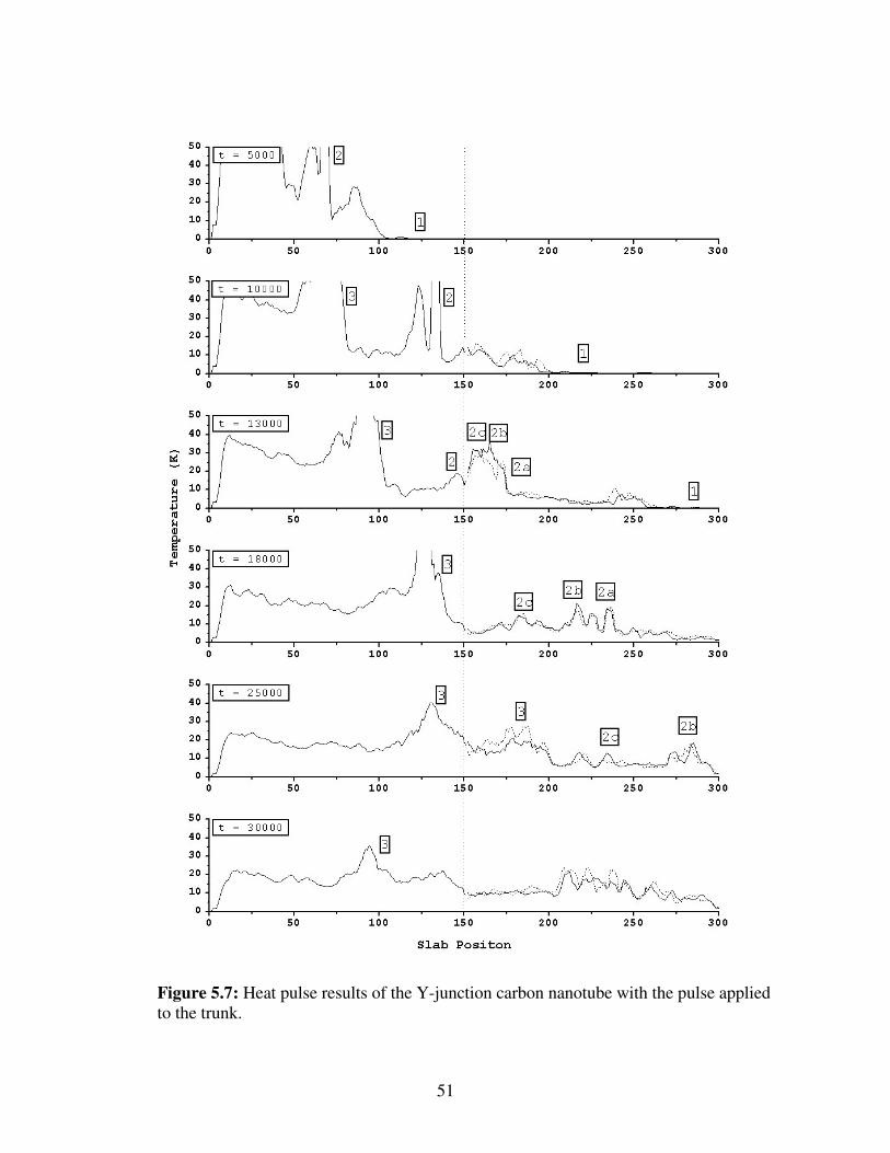
51

Figure 5.7: Heat pulse results of the Y-junction carbon nanotube with the pulse applied to the trunk.

52

transferred very well into the trunk from the branches. Each wave is made up of a distribution of

atomic vibrations. Although two waves may reach the junction at the same time, it is not

expected that the vibrations associated with these waves will be in phase with one another, and

thus interference will occur, blocking heat from flowing from the branches to the trunk. When

heat is passing from the trunk to the branches, the phase nature of the atomic vibrations is not

important because the trunk is the only source of heat. Thus, the traveling waves pass more

easily from the trunk into the branches.

In figures 5.5-5.7 it was seen that traveling waves could split into several new waves

upon passing through the junction. Each of these new waves traveled at a velocity less than or

equal to the original wave. This suggests that traveling waves can act as a heat source at the

junction, but that their inherent energy content limits which new waves can be generated. It is

also possible that a traveling wave’s orientation will determine which waves are generated when

it hits the junction. Extra molecular dynamics code would have to be written to determine

whether a traveling wave consists of longitudinal vibrations, transverse vibrations, or some

combination of the two.

In figure 5.5 it was seen that the magnitudes of the type-2 waves in the branches are

significantly different. Furthermore, their magnitudes are much smaller than the magnitude of

the type-2 wave seen in the straight (7,0) nanotube in figure 5.3. Figure 5.7 indicates that

traveling waves are transmitted very well from the trunk to the branches. However, an earlier

simulation showed that this was not the case; the traveling waves in the trunk had mostly died

out by the time they reached the junction. The newer simulation was used in this case because

the Y-junction nanotube was quenched to 0 K for a longer period of time; there was still some

thermal noise in the prior simulation. Other simulations of the straight (14,0) nanotube have

53

resulted in a type-2 wave that was nearly nonexistent. Figures 5.5 and 5.7 seem to indicate that

traveling waves pass through the junction better when they originate in the trunk. However, this

may only appear to be the case because the magnitudes of the waves that reach the junction in

figure 5.7 are much greater than those in figure 5.5.

There appears to be a good deal of inconsistency in the magnitude and stability of the

waves that are generated by the heat pulse. The cause of these issues seems to lie with the initial

state of the carbon nanotube being simulated. Before a heat pulse is applied, the nanotube is

quenched to a temperature negligibly above 0 K. This quenching is done with the application of

friction and random forces, as is done with the buffer slabs in figure 4.2. It has been observed

that a carbon nanotube quenched for a certain number of time steps will have a different heat

pulse response than the same nanotube quenched for a different number of time steps. Because

these nanotubes have been quenched for a different number of time steps, the velocities of the

atoms in the pulse slabs will most likely have different random distributions. When velocity

scaling is applied to generate the heat pulse, these velocities will be scaled to very large values.

So, while the differences in initial conditions may not matter at low temperatures, they appear to

matter when the pulse is applied.

54

CHAPTER SIX

CONCLUSION

Molecular dynamics simulations have been used to examine the thermal properties of a

Y-junction carbon nanotube under steady state and transient conditions. The steady state

simulations have revealed that the thermal conductivity of a Y-junction carbon nanotube is less

than that of a corresponding straight nanotube. This drop in thermal conductivity is the result of

the interruption of lattice continuity at the junction. The junction acts to impede heat flow by

suppressing the density of phonon modes in the system. This manifests itself in the form of a

discontinuity in the temperature profile of the Y-junction nanotube. Furthermore, it has been

found that the thermal conductivity is independent of the direction of heat flow. This is in

contrast to results obtained for electrical current flow. The calculations involving electrical

rectification included the effects of quantum electronic states. At room temperature, enough

phonon modes have been excited that the thermal properties of carbon nanotubes appear to be

continuous in nature. Furthermore, the method of simulation used in this research is entirely

classical, and does not account for the contribution of individual phonon modes. However,

experiments have indicated the existence of quantized thermal conductance at very low

temperatures. Therefore, a method of simulation that accounts for quantum thermal effects may

reveal thermal rectification at low temperatures.

The heat pulse simulations have revealed that some asymmetry in heat flow appears to

occur. Traveling waves were shown to pass fairly well from the trunk to the branches, but not so

well in the opposite direction. This was attributed to atomic vibrations of a wave in one branch

being out of phase with those in the other branch when they reached the junction. Diffusive heat

flow appeared to be limited in both directions. It was also seen that it is possible for a wave to

55

split into several waves when passing through the junction. The velocities of the new waves

were always less than or equal to the velocities of the original wave. Finally, it was noted that

there were significant inconsistencies in the magnitude and stability of the waves generated by

the heat pulse. These were attributed to variations in the initial state of the carbon nanotube that

get blown up when the heat pulse is applied.

There are several possibilities for future work. First, the steady state simulations could be

adapted to determine if thermal rectification does occur at very low temperatures. These

simulations will have to account for the individual contribution of phonons to heat flow. For the

heat pulse simulations, extra code could be added to determine the orientation of the various

modes that propagate through the nanotubes. In addition, the issue of initial conditions in the

nanotubes needs to be addressed. Finally, all of these simulations can be run again using other

Y-junction nanotubes.

56

REFERENCES 1 G. D. Hutcheson, “The First Nanochips,” Scientific American 290, Issue 4, 76 (2004). 2 S. Iijima, “Helical microtubules of graphitic carbon,” Nature 354, 56 (1991). 3 R. Saito, M. Fujita, G. Dresselhaus and M.S. Dresselhaus, “Electronic structure of graphene tubules based on C60,” Physical Review B 46, 1804 (1992). 4 N. Hamada, S. Sawada and A. Oshiyama, “New One-Dimensional Conductors: Graphitic Microtubules,” Physical Review Letters 68, 1579 (1992). 5 S. Berber, Y. Kwon and D. Tománek, “Unusually High Thermal Conductivity of Carbon Nanotubes,” Physical Review Letters 84, 4613 (1996). 6 M. Menon and D. Srivastava, “Carbon Nanotube ‘T Junctions’: Nanoscale Metal-Semiconductor-Metal Contact Devices,” Phys. Rev. Lett. 79, 4453 (1997). 7 M. Menon and D. Srivastava, “Carbon nanotube based molecular electronic devices,” J. Mat. Res. 13, 2357 (1998). 8 M. Terrones, F. Banhart, N. Grobert, J.-C Charlier, H. Terrones, and P. M. Ajayan, “Molecular Junctions by Joining Single-Walled Carbon Nanotubes,” Phys. Rev. Lett. 89, 75505 (2002). 9 L. Jing, C. Papadopolous, and J. Xu, “Growing Y-junction carbon nanotubes,” Nature 402, 253 (1999). 10 A. Andriotis, M. Menon, D. Srivstava and L. Chernozatonskii, “Transport properties of single-wall carbon nanotube Y junctions,” Physical Review B 65, 165416 (2002). 11 C. Papadopoulos, A. Rakitin, J. Li, A.S. Vedeneev and J.M. Xu, “Electronic Transport in Y-Junction Carbon Nanotubes,” Physical Review Letters 85, 3476 (2000). 12 R. Saito, G. Dresselhaus and M.S. Dresselhaus, Physical Properties of Carbon Nanotubes, Imperial College Press, London (1998). 13 V. Crespi, “Relations between global and local topology in multiple nanotube junctions,” Physical Review B 58, 12671 (1998). 14 R. Saito, M. Fujita, G. Dresselhaus and M.S. Dresselhaus, “Electronic structure of chiral graphene tubules,” Applied Physics Letters 60, 2204 (1992). 15 T.W. Odom, J. Huang, P. Kim and C.M. Lieber, “Atomic structure and electronic properties of single-walled carbon nanotubes,” Nature 391, 62 (1998). 16 L. Chico, V.H. Crespi, L.X. Benedict, S.G. Louie and M.L. Cohen, “Pure Carbon Nanoscale Devices: Nanotube Heterojunctions,” Physical Review Letters 76, 971 (1996).

57

17 Z. Yao, H.W. Postma, L. Balents and C. Dekker, “Carbon nanotube intramolecular junctions,” Nature 402, 273 (1999). 18 C. Kittel, Introduction to Solid State Physics, John Wiley and Sons, New York (1996). 19 J. Hone, M. Whitney, C. Piskoti and A. Zettl, “Thermal conductivity of single-walled carbon nanotubes,” Physical Review B 59, 2514 (1999). 20 M.A. Osman and D. Srivastava, “Temperature dependence of the thermal conductivity of single-wall carbon nanotubes,” Nanotechnology 12, 21 (2001). 21 J. Che, T. Cagin and W.A. Goddard III, “Thermal conductivity of carbon nanotubes,” Nanotechnology 11, 65 (2000). 22 J. Hone, M.C. Llaguno, N.M. Nemes and A.T. Johnson, “Electrical and thermal transport properties of magnetically aligned single wall carbon nanotube films,” Applied Physics Letters 77, 666 (2000). 23 P. Kim, L. Shi, A. Majumdar and P.L. McEuen, “Thermal Transport Measurements of Individual Multiwalled Nanotubes,” Physical Review Letters 87, 215502 (2001). 24 L.G.C. Rego and G. Kirczenow, “Quantized Thermal Conductance of Dielectric Quantum Wires,” Physical Review Letters 81, 232 (1998). 25 K. Schwab, E.A. Henrikson, J.M. Worlock and M.L. Roukes, “Measurement of the quantum of thermal conductance,” Nature 404, 974 (2000). 26 J. Hone, B. Batlogg, Z. Benes, A.T. Johnson and J.E. Fischer, “Quantized Phonon Spectrum of Single-Wall Carbon Nanotubes,” Science 289, 1730 (2000). 27 D.C. Rapaport, The Art of Molecular Dynamics Simulation, Cambridge University Press, Cambridge (1995).

28 M.P. Allen and D.J. Tildesley, Computer Simulation of Liquids, Clarenden Press, Oxford (1987).

29 J. Tersoff, “New empirical approach for the structure and energy of covalent systems,” Physical Review B 37, 6991 (1988).

30 J. Tersoff, “Empirical Interatomic Potential for Carbon, with Applications to Amorphous Carbon,” Physical Review Letters 61, 2879 (1988).

31 D.W. Brenner, “Empirical potential for hydrocarbons for use in simulating the chemical vapor deposition of diamond films,” Physical Review B 42, 9458 (1990).

58

32 C. Kittel and H. Kroemer, Thermal Physics, W.H. Freeman and Company, New York (1980). 33 D.A. McQuarrie, Statistical Mechanics, Harper and Row, New York (1976).

34 C. Oligschleger and J.C. Schön, “Simulation of thermal conductivity and heat transport in solids,” Physical Review B 59, 4125 (1999).

35 F. Müller-Plathe, “A simple nonequilibrim molecular dynamics method for calculating thermal conductivity,” Journal of Chemical Physics 106, 6082 (1997). 36 D.J. Evans and G.P. Morriss, Statistical Mechanics of Nonequilibrium Liquids, Academic Press, London (1990). 37 A. Maiti, G. Mahan, and S. Pantelides, “Dynamical simulations of nonequilibrium processes – heat flow and the Kapitza resistance across grain boundaries,” Solid State Communications 102, 517 (1997). 38 S. Maruyama, Y. Taniguchi, and Y. Shibuta, “Characterization of Heat Conduction of Carbon Nanotube by Molecular Dynamics Method,” Eurotherm 75, Champagne (2003). 39 R. Berman, Thermal Conduction in Solids, Clarendon Press, Oxford (1976). 40 R. Saito, T. Takeya, T. Kimura, G. Dresselhaus and M.S. Dresselhaus, “Raman intensity of single-wall carbon nanotubes,” Physical Review B 57, 4145 (1998).