Mohammad Hossein Khakbaz - Madjid Tavanatavana.us/publications/IJSOM.pdf · Mohammad Hossein Khakbaz ... Supplier selection decisions affect various functional areas from procurement

Int. J. Services and Operations Management, Vol. 7, No. 3, 2010 351

A multicriteria decision model for supplier selection in portfolios with interactions

Mohammad Hossein Khakbaz Department of Industrial Engineering Tarbiat Modares University Tehran, Iran E-mail: [email protected]

Amir Hossein Ghapanchi School of Information Systems, Technology and Management The University of New South Wales Sydney, Australia E-mail: [email protected]

Madjid Tavana* La Salle University Philadelphia, PA 19141, USA Fax: (267) 295–2854 E-mail: [email protected] *Corresponding author

Abstract: Supplier evaluation and selection problems are inherently multicriteria decision problems. Numerous analytical techniques ranging from simple weighted scoring to complex mathematical programming approaches have been proposed to solve these problems. However, traditional supplier selection models too often fail to consider the interaction and the capacity interdependency among the suppliers. Suppliers may exhibit internal interactions if the evaluation criteria used for one supplier are believed to be significantly affected by the evaluation criteria used by one or more of the other suppliers in the group. We propose a new branch-and-bound algorithm that generates portfolio alternatives based on Data Envelopment Analysis (DEA). The DEA model proposed in this study evaluates alternative supplier portfolios with a multicriteria model that considers possible interactions among the suppliers.

Keywords: supplier interaction; supply chain management; data envelopment analysis; DEA; supplier selection; multicriteria decision making; MCDM; weighted sum; portfolio modelling.

Reference to this paper should be made as follows: Khakbaz, M.H., Ghapanchi, A.H. and Tavana, M. (2010) ‘A multicriteria decision model for supplier selection in portfolios with interactions’, Int. J. Services and Operations Management, Vol. 7, No. 3, pp.351–377.

Copyright © 2010 Inderscience Enterprises Ltd.

352 M.H. Khakbaz, A.H. Ghapanchi and M. Tavana

Biographical notes: Mohammad Hossein Khakbaz is a Lecturer at the Azad Islamic University in Iran. He has been a distinguished Researcher at several Iranian banking research and development centres. He received his Master in Social and Economic Systems Engineering from Tarbiat Modares University and his Bachelor in Industrial Engineering from Iran University of Science and Technology. He has published in the International Journal of Business Performance Management, International Journal of Logistics Systems and Management, International Journal of Advanced Manufacturing Technology and International Journal of Information Systems and Change Management.

Amir Hossein Ghapanchi is a PhD student in Information Systems at the School of Information Systems, Technology and Management at the University of New South Wales, Australia. He holds an MS in Information Technology Engineering and a BS in Industrial Engineering. His research interests include IS human resource management, e-government planning, multicriteria decision making, supply chain management and business process reengineering. He has published in the International Journal of Information Management, International Information & Library Review, International Journal of Information Systems and Change Management, Electronic Government, an International Journal and International Journal of Public Information Systems.

Madjid Tavana is a Professor of Management Information Systems and Decision Sciences and the Lindback Distinguished Chair of Information Systems at La Salle University, USA where he served as Chairman of the Management Department and Director of the Center for Technology and Management. He has been a distinguished faculty fellow at NASA’s Kennedy Space Center, NASA’s Johnson Space Center, the Naval Research Laboratory–Stennis Space Center and the Air Force Research Laboratory. He was awarded the prestigious Space Act Award by NASA in 2005. He holds an MBA, a PMIS, and a PhD in Management Information Systems. Dr. Tavana received his postdoctoral diploma in strategic information systems from the Wharton School of the University of Pennsylvania. He is the Editor-in-Chief for the International Journal of Applied Decision Sciences and the International Journal of Strategic Decision Sciences. He has published in journals such as Decision Sciences, Interfaces, Information Systems, Information and Management, Computers and Operations Research, Journal of the Operational Research Society and Advances in Engineering Software, among others.

1 Introduction

The rapid evolution of information technology and global competition has drastically increased organisational awareness and responsiveness to customer needs. The constant pressure for customer satisfaction and competitive advantage has forced organisations to search for effective supplier selection strategies (Chou and Chang, 2008). The purpose of supplier selection is to determine the optimal supplier who can offer the best products or services for the customer. Effective supplier evaluation and selection strategies can directly impact supply chain performance resulting in organisational productivity and profitability. Numerous analytical techniques ranging from simple weighted scoring to complex mathematical programming approaches have been proposed to solve these problems. However, traditional supplier selection models too often fail to consider the interaction and the capacity interdependency among the suppliers.

A multicriteria decision model for supplier selection 353

Supplier selection decisions affect various functional areas from procurement of raw

materials and components to production and delivery of the end products. The criticality of supplier selection is evident from the significant attention in the literature and its impact on organisational performance (Banker and Khosla, 1995; Dobler et al., 1990; Srinivas et al., 2006). There are four major decisions that are related to the supplier selection problem: What product or services to order, in what quantities, from which suppliers, and in which time periods? There are two kinds of supplier selection situations: single or multiple sourcing. In single sourcing, all the suppliers can fully meet the buyer’s price, quantity, quality, and delivery requirements. Consequently, the only decision concerns the selection of the ‘best’ supplier. In contrast, Multiple sourcing is adopted when either none of the suppliers can satisfy the buyer’s total demands or when purchasing strategies aim at avoiding dependency on a single source.

The supplier evaluation and selection literature reports on numerous analytical techniques ranging from simple weighted scoring to complex mathematical programming approaches (Burke et al., 2007; Lee et al., 2001; Maltz and Ellram, 1997; Mishra and Tadikamalla, 2006). The core complexity in these techniques arises from the competing subjective and objective criteria and performance measures (Handfield et al., 2002; Purdy and Safayeni, 2000; Simpson et al., 2002). There can be little dispute that supply chain management has received a great deal of research attention in recent years. Despite the increased interest and attention, most supplier evaluation models consider suppliers as independent entities with no relation or interaction with other entities in the supply chain. The inadequate treatment of supplier interrelationships and interactions with respect to both value and resource utilisation is one of the most important limitations of the present supplier selection research.

We propose a branch-and-bound algorithm that generates alternative portfolios based on Data Envelopment Analysis (DEA). The DEA model proposed in this study evaluates alternative supplier portfolios with a multi-criteria model by considering possible interactions among the suppliers. The primary objective in this study is to consider possible interactions among the suppliers. The model identifies the most influential factors affecting supplier selection decisions and efficiently evaluates a set of alternative portfolios with interactions. The interactions between the suppliers’ performance on criteria considered in this paper is a novel approach that has not been studied in the literature. The next section presents literature review followed by a detailed explanation of our mathematical model in Section 3. In Section 4 we describe a case study and in Section 5 we present our conclusions and future research directions.

2 Literature review

Successful supply chain management requires effective sourcing strategies to protect against supply and demand uncertainties. Organisations purchase or outsource products or services from suppliers for reasons such as cost advantage, resource scarcity, insufficient capacity, inadequate time or lack of expertise. Jayaraman et al. (1999) show that single sourcing used to determine the best supplier for each purchased part can minimise the total ordering costs. However, this strategy could be detrimental to cost and quality because single suppliers may be dropped for failing to adequately perform their function and their products or services are reassigned to non-optimal


suppliers. They conclude that single sourcing is not the most effective strategy in all cases. Multiple sourcing is a useful strategy to ensure the reliability of a supplier’s supply stream. Buyers may purchase or outsource the same products or services from more than one supplier with multiple sourcing. Numerous successful organisations use multiple sourcing to fulfil their requirements and gain competitive advantage (Berger et al., 2004). Hong and Hayya (1992) show multiple sourcing frequently reduces the overall inventory and purchasing costs.

The supplier selection problem requires the consideration of multiple objectives, and hence can be viewed as a Multicriteria Decision Making (MCDM) problem (Bhutta and Huq, 2002). MCDM methods and procedures are commonly used to solve supplier selection problems (Leenders et al., 2006; Monczka et al., 2002; Talluri et al., 2006). Simple weighted rating (Ramanathan, 2007), Analytic Hierarchy Process (AHP) (Akarte et al., 2001; Bhutta and Huq, 2002; Hwang et al., 2005; Muralidharan et al., 2001; Rao, 2007; Sarkis and Talluri, 2002; Tam and Tummala, 2001; Wang et al., 2004), multi-attribute utility theory (Farzipoor Saen, 2007), mathematical programming (Amida et al., 2006), game theory (Dulmin and Mininno, 2003), neural networks (Choy et al., 2002; Choy et al., 2004), goal programming (Araz et al., 2007), decision trees (Berger and Zeng, 2006), neural networks (Ohdar and Ray, 2004), and DEA (Braglia and Petroni, 2000; Joo et al., 2009; Liu et al., 2000; Muralidharan et al., 2002; Weber et al., 1998; Weber et al., 2000) are among the most widely used MCDM methods for supplier evaluation and selection. Narasimhan et al. (2001) first used DEA to evaluate the effectiveness of the suppliers. They proposed a methodology where the efficiencies derived from their DEA model were utilised in identifying supplier clusters categorised into high performers and efficient, high performers and inefficient, low performers and efficient, and low performers and inefficient. Other researchers have also studied the application of DEA in supplier selection and negotiating with inefficient suppliers (Weber and Desai, 1996; Weber et al., 1998). Talluri et al. (2006) presented a chance-constrained DEA approach in the presence of multiple performance measures that are uncertain. They demonstrated the first application of chance-constrained DEA in the area of purchasing to a previously reported dataset from a pharmaceutical company.

Portfolios of suppliers are commonly suggested as a response to buyer’s requirements in multiple sourcing problems (Sarkis and Talluri, 2002; De Boer et al., 1998; Degraeve and Roodhooft, 2000). Portfolio models have their foundation in Markowitz’s (2002) pioneering portfolio theory for the management of equity investments. Portfolio models are routinely used in strategic planning and this trend has escalated over the past decade as purchasing management has become more strategic. The AHP is frequently used to evaluate portfolios of suppliers in multiple sourcing (Benyoucef and Canbolat, 2007). Xia and Wu (2007) have proposed an integrated AHP framework improved by rough sets theory and multi-objective mixed integer programming. Their approach considers supplier’s capacity constraints and simultaneously determines the number of suppliers and the order quantity allocated to each supplier. Other techniques such as simulation models are also used to assess and compare portfolios of suppliers within a multi-tier sourcing framework (Marquez and Blanchar, 2004).

Three key measures used widely for supplier portfolio assessment and selection are price, delivery, and quality (Buffa and Jackson, 1983; Lemke et al., 2000; Pan, 1989). Other measures such as transportation and purchasing costs, vendors’ product quality, delivery, and capacity are also proposed for supplier evaluation and selection (Bender et al., 1985; Cavinato, 1992; Merli, 1991). Single versus multiple sourcing preference


orientation of a firm has been shown to have an effect on the supplier selection criteria (Swift, 1995). Swift’s study showed that price and dependability were rated significantly different between those who have a preference for single sourcing and those who have a preference for multiple sourcing. In addition to sourcing preference, other organisational or personal factors have been shown to have an impact on supplier selection criteria.

Effective and efficient design of the supply chain is a powerful competence in improving performance and productivity. Sezen (2008) carried out an empirical study to investigate the relative effects of supply chain integration, information sharing and design on performance. He showed integration, information sharing and specifically supply chain design directly impact flexibility, resource and output performances of supply chains. Sezen (2008) suggested a very useful construct for supply chain design by developing measurements for dependent and independent variables. Dependent variables included flexibility performance, resource performance and output performance. Independent variables included supply chain integration, information sharing with suppliers, information sharing with customers and supply chain design. Some of the measurement scales for integration included the contact frequency among the firms in the supply chain and the compatibility of the information systems. Some of the measurement scales for information sharing included the capacity information sharing among the firm and its suppliers and the ability of the firm to find information about the suppliers’ products and prices.

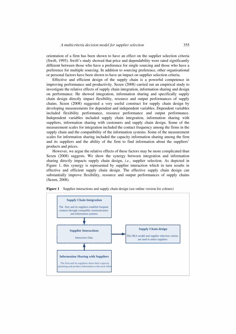
However, we argue the relative effects of these factors may be more complicated than Sezen (2008) suggests. We show the synergy between integration and information sharing directly impacts supply chain design, i.e., supplier selection. As depicted in Figure 1, this synergy is represented by supplier interaction which in turn results in effective and efficient supply chain design. The effective supply chain design can substantially improve flexibility, resource and output performances of supply chains (Sezen, 2008).

Figure 1 Supplier interactions and supply chain design (see online version for colours)

Supply Chain Integration

The firm and its suppliers establish frequent contacts through compatible communication

and information systems

Supplier Interactions

Interaction Data

Supply Chain design

The DEA model and supplier selection criteria are used to select suppliers

Information Sharing with Suppliers

The firm and its suppliers share their capacity planning and product information with each other


3 Methodology

We propose a new branch-and-bound algorithm that generates portfolio alternatives based on DEA. The DEA model proposed in this study evaluates alternative supplier portfolios with a multi-criteria model that considers possible interactions among the suppliers.

3.1 The DEA model

DEA is a mathematical programming technique that measures the relative efficiency of multiple Decision-Making Units (DMUs) based on multiple inputs and outputs (Eilat et al., 2006). The number of DMUs is represented by n, each DMU uses m inputs and produces s outputs. Inputs are represented by the vector Xj = {xij} (i = 1, . . . ,m) and outputs are represented by the vector Yj = {yrj} (r = 1, . . . , s) for project j (j = 1, . . . , n). The basic DEA model called the Charnes, Cooper and Rhodes (CCR) model was introduced by Charnes et al. (1978). In this model, A0 represents the relative weight of a particular DMU, as the ratio between the weighted-sum of the outputs to the weighted sum of the inputs. The following formulation presents the CCR model where the constant ε is an infinitesimal number that functions as a lower bound for the weights.

Max 0

0

r rr

i ii

u y

v x

∑∑

(1)

s.t. 1r rj

r

i iji

u yj

v x≤ ∀

∑∑

(2)

ru ε≥ (3)

.iv ε≥ (4)

By solving formulation (1) n times (each time evaluating a different DMU), we find the relative efficiency score of the DMUs. These measures divides the DMUs into two categories: efficient DMUs (with score of 1.0) and inefficient DMUs (with scores smaller than 1.0).

3.2 The proposed methodology

The proposed methodology (see Figure 2) is composed of five steps. It begins with the establishment of evaluation criteria through expert opinions and historical data (Step 1). A branch-and-bound model is then applied to generate alternative portfolios and each portfolios’ real capacity (the real capacity which the supplier can deliver) and actual capability (the real capacity which the supplier can deliver minus defective products) (Step 2). Subsequently, maximal portfolios are established by considering need and capacity constraints (Step 3). Next, an accumulation function that takes into account the combined effect of possible benefit, outcome, and resource interactions is constructed.


This function is then applied to the capacity, input and outputs of the candidate suppliers in each portfolio to determine aggregate portfolio inputs and outputs (Step 4). Finally, the DEA model is used to determine the most efficient portfolios (Step 5).

Figure 2 The proposed methodology (see online version for colours)

Establishing Evaluation Criteria

Generating Portfolios

DEA Model

Interaction Data

Need and Capacity Constraints

Branch and Bound Algorithm

Expert Opinions and Historical Data

Selecting the Most Efficient Portfolios

Calculating the Accumulation Function

Exploring Maximal Portfolios

Step 1 Establishing evaluation criteria

In this step, input and output criteria and indices are established by a group of experts. Alternative selection in MCDM is facilitated by evaluating each alternative on the set of criteria. The criterion outcomes provide the basis for comparison of the alternatives under consideration. Therefore, the evaluation criteria must be measurable – even if the measurement is conducted only at the nominal scale. Roy (1996) has argued that criteria in MCDM serve as a basis of a judgement. In this context, the criteria must help establish the preference judgements that form the basis of the decision. Keeney and Raiffa (1976) have suggested that the following five principles be considered when criteria are being selected: completeness (the criteria must embrace all of the essential characteristics of the decision problem), operational ability (the criteria must be meaningful), decomposability (the criteria should be decomposable), non-redundancy (the criteria should avoid duplicate measurement of the same performance), and minimum size (the number of criteria should be manageable and as small as possible). Using these guidelines, we use expert opinions and the firms’ data on historical and current proposals to identify the input, outputs, potential capacity for each supplier; and the potential interactions (including input, output, and capacity interactions) between the suppliers.

Step 2 Generating portfolios

This step is intended to generate all possible portfolios using a branch-and-bound technique. The capacity and capability of each portfolio k is also calculated using Equations (5–6). Capacity is the real capacity which the supplier can deliver and capability is the real capacity which the supplier can deliver minus defective products.


1 1

n nk k

k i ij iji j

Capacity z z w= =

⎛ ⎞= ⎜

⎝ ⎠∑ ∑ ⎟

⎞⎟⎠

(5)

1

1 1 1

.n n n

k k kk i ij ij ij ij

i j j

Capability z z w z u= = =

⎛ ⎞⎛= ⎜ ⎟⎜

⎝ ⎠⎝∑ ∑ ∑ (6)

Notations:

n the total number of suppliers. kiz the existence of supplier i in portfolio k ( 1,k

iz = if supplier i is included in portfolio k; otherwise, 0).k

iz =kijz the existence of supplier i and j in portfolio k ( k

ijz 1,= if both suppliers i and j are included in portfolio k; otherwise, 0).k

ijz =

wjk the capacity interaction between suppliers j and k (wjj represents the capacity of supplier j).

1jkv the transportation price interaction between suppliers j and k represents the

transportation price of supplier j).

1( jjv

2jkv the product price interaction between suppliers j and k represents the product

price of supplier j).

2( jjv

1jku the accepted rate interaction between suppliers j and k represents the accepted

rate of supplier j).

1( jju

2jku the on-time delivery interaction between suppliers j and k represents the

on-time delivery probability of supplier j).

2( jju

3jku the after-sale service quality interaction between suppliers j and k represents

the after-sale service quality of supplier j).

3( jju

ˆkx the average amount of input allocated to portfolio k.

ˆrky the average amount of output r allocated to portfolio k.

Step 3 Exploring maximal portfolios

A portfolio of suppliers is said to be maximal, if the following two conditions hold:

1 The portfolio capacity is in the range of our minimum and maximum needs

2 Any additional supplier inclusion in the portfolio violates the capacity constraints.

In this step, we model the maximal portfolios as DMUs with specified capacity, input and outputs. To compute the values of capacity, input and outputs for a portfolio as a whole, we use the accumulation function presented in the next step.

Step 4 Calculating the accumulation function

Internal interactions can be further classified into three categories: input interactions, output interactions, and capacity interactions. Input interactions may occur if the total resource requirements of suppliers in the portfolio cannot be represented as the sum of resources of the individual suppliers. This might occur in different situations. For


example, ordering suppliers located in the same geographical location could decrease transportation cost. Also, competition or having a shared board of directors can reduce product price.

Output interactions may occur if the inclusion of two suppliers in a portfolio results in an output which is not equal to the sum of the outputs of the two suppliers. For example, ordering suppliers located in the same geographical location can affect their product accepted rates, delivery times, and after-sale services. Typically, in those cases where suppliers have the same board of directors, they share their capacities to increase their service level and in those cases where the suppliers have the same service provider, their service could potentially decrease. Additionally, competition between suppliers can force them to make higher quality products, and consequently, more accepted rate. Moreover, on-time delivery interactions may occur if the suppliers use the same transportation facilities or have a shared management team that schedules the delivery programme. Usually, having shared transportation facilities can decrease the on-time delivery probability and having a shared management team for a scheduling delivery programme can reduce delivery time.

Capacity interactions may occur if a supplier capacity depends on the other. Generally, if we place an order with two suppliers in the same region, their total capacity could decrease because of the shared and limited resources in the region. Equations (7–10) provide a general accumulation function for all combined input, outputs, and capacity interactions. To account for the input interaction, let and be respectively, the transportation and purchasing price interaction between suppliers i and j. If suppliers i and j are both in a portfolio, and will be added to the transportation and purchasing prices of supplier i. and represent the transportation and purchasing price of supplier j. Similarly, and represent the accepted rate, on-time delivery probability, and after-sale service quality level interactions between suppliers i and j. The average amount of input required for portfolio k, is presented by following equation:

1ijv 2

ijv

1ijv 2

ijv1jjv 2

jjv1 ,iju 2 ,iju 3

iju

1 2

1 1 1

( )

ˆ .

n n nk k ki ij ij ij ij ij

i j j

kk

z z w z v v

xcapacity

= = =

⎛ ⎞⎛+⎜ ⎟⎜

⎝ ⎠⎝=∑ ∑ ∑

⎞⎟⎠ (7)

Also, the average amounts of output r allocated to portfolio k, are presented in Equation (10):

ˆ ,rky

1ˆ k

kk

capabilityy

capacity= (8)

1 2

1 1 1 1

2ˆ

n n n nk k k ki ij ij ij ij ij i

i j j j

kk

jz z w z u z u

ycapability

= = = =

⎛ ⎞⎛ ⎞⎛ ⎞⎜ ⎟⎜ ⎟⎜ ⎟⎝ ⎠⎝ ⎠⎝=

∑ ∑ ∑ ∑⎠ (9)

1 3

1 1 1 1

3ˆ .

n n n nk k k ki ij ij ij ij ij ij

i j j j

kk

z z w z u z u

ycapability

= = = =

⎛ ⎞⎛ ⎞⎛ ⎞⎜ ⎟⎜ ⎟⎜ ⎟⎝ ⎠⎝ ⎠⎝=

∑ ∑ ∑ ∑⎠ (10)


After modelling the portfolios as DMUs, the DEA model is used to find the relative values that reflect the overall attractiveness of the portfolios.

Step 5 Selecting the most efficient portfolios

In this step, the DEA model is applied on maximal portfolios. Each portfolio has an input ( ) and three outputs 1 2 and 3 By solving this model n times (each time evaluating a different maximal portfolio), we find the relative efficiency scores of all DMUs. These measures divide the DMUs into two categories: efficient DMUs (with a score of 1.0) and inefficient DMUs (with scores smaller than 1.0).

ˆkx ˆ( ,ky ˆ ,ky ˆ ).ky

4 The case study

We use the following case study to illustrate some of the numerical aspects of the proposed methodology. The buyer is Iran Motors Industrial Group,1 a major Iranian industrial manufacturer. The company manufactures cars for the domestic and export markets. Iran Motors has a long-term relationship with Peugeot Citroën and assembles several Peugeot models under license from the French firm. The company also makes trucks, buses, and passenger cars under license from Mercedes-Benz.

The suppliers are a set of ten steel sheet vendors in four different regions. The demand forecast indicates a need for 2000 to 2200 sheets of steel in the next period. The existing supplier selection models, from linear programming to neural networks, could not be used for portfolio selection because of the high level of interdependency among the suppliers, especially among those located in the same region. While considering supplier interactions adds significantly to the complexity of the model, not considering the interdependencies may result in less than optimal solutions for decision variables such as scheduling of the production line and budget allocation.

Step 1 Establishing evaluation criteria

A group of 15 supply chain management experts from Iran Motors were selected to participate in this study. The Delphi method was utilised to collect and synthesise expert opinions. The Delphi method is based on a structured process for collecting and synthesising knowledge from a group of experts by means of a series of questionnaires combined with controlled opinion feedback (Adler and Ziglio, 1996). The group held several brainstorming sessions to discuss the relevant criteria for selecting suppliers. Several anonymous questionnaires were administered in the form of an iterative consultation procedure. Product price, accepted rate, on-time delivery, and vendor’s after-sale service were identified as the four most important factors in evaluating alternative suppliers throughout the Delphi process.

Product price represents the direct purchasing cost of an item on a unit basis. Accepted rate represents the percentage of shipped units that are accepted by the buyer. On-time delivery is measured as the percentage of ordered units that are delivered on-time. After-sale service is the supplier’s quality of service to support products. Moreover, the Delphi method identified the total price (purchase price plus transportation cost per unit) as the input factor, and the accepted rate, on-time delivery, and the after-sale service as the output factors. Furthermore, product price was considered as an


input factor because it represent the amount paid by the buyer while accepted rate, on-time delivery, and service performance were considered as output factors because they represented the benefits gained by the buyer. Based on our model convention, higher values of outputs and lower values of inputs are considered desirable. The measures for the accepted rate and on-time delivery are from [0, 1] and after-sale service is measured in terms of a percentage. Although we assumed the three outputs are equal in importance, the model could easily be generalised to consider various weights for each of these factors. The importance weight associated with each factor can be elicited by different weighting procedures. The simplest approach is weighting each factor directly by point allocation. Other weighting methods include SMART and SMARTER (Barron and Barnett, 1996; Edwards and Barron, 1994), SWING (Von Winterfeldt and Edwards, 1986), and AHP (Saaty, 2005). Using SMART, ten points are given to the least important factor. Then, more points are given to the other factors, depending on their relative importance. In SMARTER, the weights are elicited with the centroid method of Solymosi and Dombi (1986). The SWING method is similar, but the procedure starts from the most important factor, keeping it as the reference. In AHP, the weights are derived by comparing all the factors to one another in pairs. Table 1 shows the suppliers data derived from the firms’ historical data and proposals.

Table 1 Suppliers and interaction data

Supplier number

Capacity wjk

Transportation price

(dollars) 1jkv

Product price

(dollars)

2jkv

Accepted

rate 1jku

On-time delivery

2jku

Service

3jku

1 870 92 745 0.92 0.74 76.4 2 640 74 850 0.91 0.71 67.8 3 770 97 815 0.71 0.71 66.4 4 520 113 760 0.89 0.67 71.2 5 890 102 845 0.75 0.64 82.4 6 620 69 875 0.77 0.91 77.8 7 580 76 840 0.62 0.85 95.4 8 760 89 770 0.87 0.88 79.8 9 530 92 890 0.68 0.79 75.4 10 360 105 900 0.81 0.81 86.4

Next, we illustrate the interactions among the suppliers through capacity, quality, transportation cost, on-time delivery, service performance, and price interdependencies.

Capacity interdependency

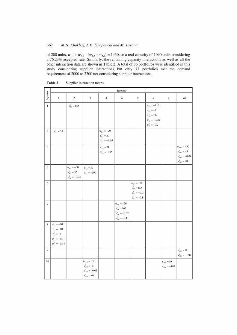
The capacity interdependency among the suppliers was noticeably high. For example suppliers 1 and 8 were both located in the Azerbaijan providence in northwestern Iran and used a common source for their raw materials. Selection of both suppliers in a portfolio could potentially decrease their capacity. For example, suppliers 1 and 8 each could supply 870 and 760 units independently. However, when both were selected in the same portfolio, supplier 1 capacity decreased from 870 to 760 (w1,8 = –110) while supplier 8 capacity decreased from 760 to 670 (w8,1 = –90) resulting in a total reduction


of 200 units, w1,1 + w8,8 – (w1,8 + w8,1) = 1430, or a real capacity of 1090 units considering a 76.23% accepted rate. Similarly, the remaining capacity interactions as well as all the other interaction data are shown in Table 2. A total of 86 portfolios were identified in this study considering supplier interactions but only 77 portfolios met the demand requirement of 2000 to 2200 not considering supplier interactions.

Table 2 Supplier interaction matrix

Supplier

Supp

lier

1 2 3 4 6 7 8 9 10

1 21,2 155v = 1,8

11,8

21,8

11,8

21,8

110

7

192

0.08

0.2

w

v

v

u

u

= −

= −

=

= −

= −

2 22,1 55v = 2,4

12,4

12,4

20

20

0.05

w

v

u

= −

=

= −

3 33,4

23,4

31

195

u

v

=

= −

3,10

13,10

13,10

23,10

30

5

0.04

0.1

w

v

u

u

= −

= −

= −

= +

4 4,2

14,2

14,2

30

32

0.04

w

v

u

= −

=

= −

34,3

24,3

32

190

u

v

=

= −

6 6,7

26,7

16,7

26,7

30

188

0.01

0.11

w

v

u

u

= −

=

= −

= +

7 7,6

27,6

17,6

27,6

20

167

0.02

0.11

w

v

u

u

= −

=

= −

= +

8 8,1

18,1

28,1

18,1

28,1

90

10

15

0.1

0.14

w

v

v

u

u

= −

= −

=

= −

= −

9 39,10

29,10

18

188

u

v

=

= −

10 10,3

110.3

110,3

210,3

30

5

0.05

0.1

w

v

u

u

= −

= −

= −

= +

310,9

210,9

19

197

u

v

=

= −


1 1 1 1w u w u w u w u× + × + × + ×

1 w′

Consider the requirement of 2000 to 2200 sheets of steel in the next period. There was a possibility that some portfolios supplying over the maximum limit of 2200 units would be omitted from consideration but in reality the actual supply could end up less than this maximum limit because of the interaction among the suppliers. Let us consider the following situation where we first defined all portfolios that supplied between 2000 to 2200 units. Not considering the interaction among the portfolios could have resulted in eliminating portfolios not meeting the minimum requirement. For example, portfolio 0101100001 providing 2004 units could only supply 1909 units because of the interaction between suppliers 2 and 4. We received and paid for w2,2 + w4,4 + w5,5 + w10,10 + w2,4 + w42 or 2360 units but we could only use or 2004 units in the production line not considering interactions. However, after considering capacity and quality interactions between suppliers 2 and 4, the real supply was w u

2,2 2,2 4,4 4,4 5,5 5,5 10,10 10,10

2,2 2,2 4,4′ ′× + ×

1 1 1u w u w u′ + × + × 620;w w w

or 1909 units where 4,4 55 55 10,10 10,10 2,2 2,2 2,4′ = + = w w′ = +

490;w = 1 0.86;u u u′ = + = 1 0.85.u u u′ = + =

and In contrast, there were other cases where a portfolio did not meet our minimum or maximum requirements and was consequently dropped out of the set but considering the interaction among the suppliers, the portfolio would have met the minimum and maximum requirements. The remaining capacity interactions among the ten suppliers are shown in Table 2. It should be noted that supplier 5 is not in Table 2 because that supplier has no interactions with the other 9 suppliers in the set.

4,4 4,4

4,2 2,2 2,2 2,4 4,4 4,4 4,2

Quality interdependency

Quality interaction represented by the accepted rates (percentage of shipped units that are not rejected) is also an important factor, especially, when suppliers rely on a common source. For example, placing an order with both suppliers 2 and 4 in portfolio 0101100001, reduced the accepted rate of supplier 2 from 0.91 to 0.86 ( and similarly reduced the accepted rate of supplier 4 from 0.89 to 0.85. Consequently, the average accepted rate dropped from 0.83 to 0.80. Given and the average accepted rate without interaction was ( or 1959.4/2360 = 0.83; and, given and the average accepted rate with interaction was

1 1 12,2 2,2 2,4 0.91 0.05 0.86)u u u′ = + = − =

12,2 0.91u = 1

4,4 0.89,u =1 1 1 1

2,2 2,2 4,4 4,4 55 55 10,10 10,10 ) /w u w u w u w u W′ ′× + × + × + ×1 1 12,2 2,2 2,4 0.91 0.05 0.86u u u′ = + = − = 1 1 1

4,4 2,2 4,2 0.89 0.04 0.85,u u u′ = + = − =1 1 1

2,2 2,2 4,4 4,4 55 55 10,10(w u w u w u w′ ′′ ′× + × + × + ×W

or 0.80. 1

10,10 ) /uMoreover, consider a situation where suppliers in one geographical region purchased

their raw materials from the same source. For example suppliers 1 and 8 in northern Iran both purchased their raw iron from the same iron mine. When we placed an order with both suppliers, their combined order put a burden on the supplier of the raw iron which in turn affected the quality of the raw materials and ultimately the quality of the final products (steel sheets). In summary, placing an order with two suppliers might have a downside or upside effect on the capacity and quality. For example, in portfolio 0101100001 where the capacity reduced from 2004 to 1909 and the average accepted rate reduced from 0.83 to 0.80.


Transportation cost interdependency

Transportation cost interdependency also played an important role in the portfolio selection. For example, placing an order with suppliers 2 and 4 separately resulted in a higher transportation cost than placing a joint order with both suppliers. Suppliers 2 and 4 were located in the Zahedan providence in southern Iran where the transportation infrastructure is underdeveloped. Small freight shipment from this region is generally limited and expensive. Placing an order with the two suppliers in this region increased the total transportation cost). The transportation cost per unit for supplier 2 increased by 20 dollars from 74 dollars to 94 dollars per unit and the transportation cost for supplier 4 increased by 32 dollars from 113 dollars to 145 dollars per unit. The total transportation cost for portfolio 0111000100 not considering supplier interaction was

dollars given and while the total cost considering supplier interaction resulted in a total transportation cost of

dollars given

12,4( 2v = + 0) )

2))

×

1 1 12,2 2,2 2,4(v v v′ = +

14,2( 3v = +

1 1 14,4 4,4 4,2(v v v′ = +

12,2 2,2 3,3w v w′ × +

1 1 13,3 4,4 4,4 8,8 8,8 243,580′′+ × + × =v w v w v 1

2,2 74v = 14,4 113v =

1 1 1 12,2 2,2 3,3 3,3 4,4 4,4 8,8 8,8 271,660′ ′′ ′× + × + × + × =w v w v w v w v 1

2,2 74 20 94v ′ = + = and On the contrary, it was also possible for the suppliers to combine their shipments and receive volume discount from the freight forwarders. For example, suppliers 1 and 8 were able to combine their shipments and reduce their transportation cost from 92 dollars to 85 dollars per unit for supplier 1 and from 89 dollars to 79 dollars per unit for supplier 8

14,4 113 32 145.v ′ = + =

11,8(v = −7)

0).

w u w u w u w u W′ ′′ ′× + × + × + × = 2 0.74,= 2 0.88,u =

18,1( 1v = −

On-time delivery interdependency

Purchasing from suppliers in the same geographical region sometimes resulted in an increase in on-time delivery, especially, when there was a scarcity of resources and lack of manpower in the region. On time delivery is measured as the percentage of ordered units that are not delayed. For example, every time an order was placed with both suppliers 6 and 7 located in the Khorasan providence in northeastern Iran, there was delay in the delivery of the products because both suppliers relied on shared resources and could not fulfil the order in a timely fashion. On the contrary, the interaction among the suppliers sometimes lowered the expected on time delivery. Let us consider portfolio 1100000101 where not considering supplier interaction showed an on-time delivery of

where 1,1u 8,8

1,1 1,1 1,8 and 8,8 8,8 8,1

2 2 2 21,1 1,1 2,2 2,2 8,8 8,8 10,10 10,10( ) / 0.81

760,w w w′ = + = 770.w w w′ = + = However, the real delivery, considering the interaction between suppliers 1 and 8, was 2 2

1,1 1,1 2,2 2,2w u w u′′ × + × + where

and

2 28,8 8,8 10,10 10,10 ) / 0.65w w w u W′′ × + × = 2 2 2

1,1 1,1 1,8 0.54,u u u′ = + = 2 2 28,8 8,8 8,1 0.74,u u u′ = + =

1,1 1,1 1,8 760,w w w′ = + = 8,8 8,8 8,1 770.w w w′ = + =

Service performance interdependency

Service performance, measured using a 1-100 scale, was also affected by the interaction among the suppliers. For example, suppliers 3 and 4 had a contractual agreement to provide after-sale service. Putting both suppliers in the portfolio resulted in an increase in the average after-sales service since both suppliers used a common system for loading, unloading, and identification of the damaged products. For example, the average service performance in portfolio 0111000100 without considering interaction was where 3,3 and

while the average service performance without considering interaction

3 3 3 32,2 2,2 3,3 3,3 4,4 4,4 8,8 8,8( ) / 70.2w u w u w u w u W′ ′× + × + + + × = 3 66.4u =

34,4 71.2u =


resulted in an increase in on-time delivery from 70.2 to 84.4 or

where and

32,2 2,2(w u′ × +

3 3 33,3 3,3 4,4 4,4 8,8 8,8 ) /w u w u w u W′ ′′× + × + × 3 3 3

3,3 3,3 3,4 66.4 31 97.4u u u′ = + = + =3 3 34,4 4,4 4,3 71.2 21 92.2.u u u′ = + = + =

Price interdependency

The price interdependency was also noticeable because of the competition among the suppliers. For example, when we placed an order with suppliers 3 and 4, both offered a discounted price and the total cost decreased. In addition, placing an order with two suppliers with unmatchable specifications in the portfolio was also sometimes effective. For example, we used 207 dollars to match products with unmatchable specifications supplied by suppliers 1 and 8 since the steel sheet specifications did not match. Let us consider portfolio 1100000101 where the width of two roles coming from suppliers 1 and 8 were not identical. In order to match these roles of steel, we were required to spend 192 dollars on the steel sheets supplied by supplier 1 and 15 dollars on the sheets supplied by supplier 8. The total purchase price without considering interaction was

dollars where and whereas considering the interaction between suppliers 1 and 8, the total

purchase price was dollars, where and On the contrary, we considered portfolio 0111000100 where an order placed with both supplier 3 and 4, resulted in a reduced total price of

2 2 2 21,1 1,1 2,2 2,2 8,8 8,8 10,10 10,10 2,027,100′ ′′ ′× + × + × + × =w v w v w v w v 2

1,1 745v =28,8 770v =

2 2 2 21,1 1,1 2,2 2,2 8,8 8,8 10,10 10,10 21,845,570′ ′′ ′× + × + × + × =w v w v w v w v

2 2 21,1 1,1 1,8 937v v v′ = + = 2 2 2

8,8 8,8 8,1 770 15 785.v v v′ = + = + =

2 2 22,2 2,2 3,3 3,3 4,4 4,4 8,8

′ ′′ ′× + × + × +w v w v w v w × dollars where and 2

8,8 1, 716,900=v 2 2 23,3 3,3 3,4 620v v v′ = + = 2 2 2

4,4 4,4 4,3 570.v v v′ = + =

Step 2 Generating portfolios

This step generated all possible portfolios using the branch-and-bound technique. The capacity and capability of each portfolio were also calculated using Equations (5–6).

Step 3 Exploring maximal portfolios

All ten steel sheet suppliers in this study had a capability constraint that was more than 2000 and less than 2200 units. In this step, all possible portfolios that met this constraint were identified. The maximal number of portfolios satisfying this constraint was 86, with portfolios including 3 to 6 suppliers.

Step 4 Calculating the accumulation function

In this step, Equations (7–10) were used to calculate the accumulated capacity, input and outputs, taking into account the interactions. As a result for each maximal portfolio four measures were calculated: the average total price allocated to portfolio k; 1 the accumulated accepted rate allocated to portfolio k; 2 the accumulated on-time delivery probability allocated to portfolio k; and, the accumulated after-sale service quality allocated.

ˆ ,kx ˆ ,kyˆ ,ky

3ˆ ,ky


Step 5 Selecting the most efficient portfolios

Next, we applied the DEA model to evaluate the portfolios. Each portfolio had an input ( ) and three outputs 1 2 and 3 Table 3 presents the sorted portfolios (the top and bottom ten ranked portfolios). For each portfolio, the table gives its identification (a 10-digit binary vector), the corresponding capability, accumulated input and outputs, and the DEA score. These measures divided the portfolios into two categories: those with the score of 1.0 (efficient), and those portfolios with less than a 1.0 score (inefficient).

ˆkx ˆ( ,ky ˆ ,ky ˆ ).ky

Table 3 Portfolio evaluation results (sorted DEA scores) (see online version for colours)

Outputs

Sorted

portfolios Label Capacity

Total cost

(dollars) Accepted

rate On-time delivery

After-sale

service DEA score

1 1011000001 2010 1,940,230 0.82 0.77 92.52 1.000000

2 0011001100 2030 2,091,370 0.77 0.78 95.75 0.960115

3 0100010101 2013 2,191,280 0.85 0.83 77.05 0.957329

4 1001010001 2032 2,129,230 0.86 0.78 77.14 0.956381

5 0011010011 2047 2,153,130 0.75 0.81 96.77 0.954045

6 0011010100 2148 2,145,370 0.80 0.80 91.66 0.937279

7 0011000110 2031 2,080,550 0.79 0.77 91.65 0.931810

8 0111000011 2057 2,148,320 0.76 0.77 94.42 0.921667

9 1100000011 2035 2,201,300 0.85 0.75 82.21 0.914675

10 1011001000 2170 2,166,720 0.79 0.74 94.03 0.910080

....... ....... ....... ....... ....... ....... ....... ....... 78 0010110010 2052 2,650,810 0.73 0.75 75.68 0.710983

79 1000001111 2166 2,598,580 0.75 0.73 87.69 0.707688

80 1010000110 2061 2,578,300 0.76 0.69 74.22 0.695507

81 1010010100 2178 2,643,120 0.77 0.72 74.79 0.694076

82 1010001100 2061 2,589,120 0.74 0.70 78.41 0.682046

83 0110100010 2157 2,656,890 0.76 0.70 73.43 0.681280

84 0110101000 2156 2,667,710 0.75 0.72 77.50 0.677650

85 0010111001 2199 3,126,770 0.71 0.84 80.49 0.676796

86 1000100110 2182 2,718,890 0.77 0.66 78.89 0.668796

87 1000101100 2181 2,729,710 0.75 0.68 82.83 0.654420

In this case study, we identified one portfolio with the score of 1.0, and 4 portfolios with a score higher than 0.95 (see Table 3). The top portfolio is 1011000001 with suppliers 1, 3, 4, and 10. Our study revealed that the analysis does not point out a single best portfolio. Rather, it reduces the large number of potential portfolios significantly to a small and manageable number of attractive alternative choices, while integrating several seemingly different criteria. To show the importance of the interaction among the suppliers, we ran our model again without interaction consideration. The results are presented in Table 4.


Table 4 Portfolio evaluation results (without interactions) (see online version for colours)

Outputs

Sorted portfolios Label Capacity

Total cost (dollars)

Accepted rate

On-time delivery

After-sale

service DEA score

1 1100000100 2044 1,972,390 0.90 0.78 75.11 1.000000

2 0100010101 2013 2,191,280 0.85 0.83 77.05 0.961508

3 1000001101 2113 2,274,110 0.82 0.82 83.09 0.959473

4 1001010001 2032 2,129,230 0.86 0.78 77.14 0.951383

5 1100001001 2034 2,212,630 0.83 0.77 80.12 0.950847

6 1010000100 2008 2,083,270 0.84 0.77 74.27 0.942269

7 1000100100 2129 2,223,860 0.84 0.75 79.54 0.939239

8 1100100000 2050 2,162,380 0.85 0.69 76.33 0.926929

9 0101001100 2066 2,229,440 0.83 0.79 78.56 0.925275

10 1101000001 2137 2,135,310 0.89 0.73 74.47 0.917327

....... ....... ....... ....... ....... ....... ....... .......

A comparison between Tables 3 and 4 shows that portfolio 1000010100 with a supply of 2063 units can only produce 1632 units, portfolio 1001000100 with a supply of 2054 units can only produce 1617 units, and portfolio 1100000100 with 1737 units can only produce 1617 units all due to the interaction among the suppliers. A closer examination of the results further shows very little consistency among the top ten portfolios in the two lists presented in Tables 3 and 4. For example, the portfolio 1011000001 with a total cost of 1,940,230 dollars and a DEA score of 1.00 in Table 3 is not among the top 10 portfolios in Table 4. Similarly, the portfolios 0011001100, 0011010011, 0011010100, 0011000110, 0111000011, 1100000011, and 1011001000 do not appear among the top 10 portfolios in Table 4. Only 2 portfolios appear on both lists: portfolios 0100010101 with total cost of 2,191,280 dollars and portfolio 1001010001 with total cost of 2,129,230 dollars. The 2 portfolios appear on both lists because there is no interaction between suppliers 2, 6, 8 and 10; and between suppliers 1, 4, 6 and 10 (see Table 2). We should note the cost of modelling and obtaining all the data for every possible interaction is not included in the overall cost benefit assessment. However, in cases where this information is readily available or quantifiable, it should be considered in the cost function.

A sensitivity analysis was performed on the interaction categories to see how sensitive the rankings of the various portfolios were to ±5% and ±10% changes in the parameters. For example, the initial capacity values were changed by ±5% and the resulting rankings were compared to see the overall impact these changes had on the final decision. The results for the top five candidates from the list of eligible portfolios are given in Table 5. Notice that when the capacity was increased by 5%, only portfolios 1011000001 and 0011001100 remained on the top-5 list and when the capacity was decreased by 5%, the top 5 portfolios were different. We also performed a sensitivity analysis with ±10% on the capacity. When the capacity was increased by 10%, the top five portfolios were different from the top five portfolios when the capacity was reduced by 10%. Similarly, a 5% increase in the accepted rate produced different portfolios for


the top five compared with a 5% reduction in the accepted rate. Thus, the rankings were quite sensitive to small changes in the capacity and the accepted rate. Table 5 presents the partial results from the sensitivity analysis.

Table 5 Sensitivity analysis results (see online version for colours)

Outputs

Interaction

category Sensitivity range

Number

of

eligible

portfolios

Portfolio

labels Capacity

Total cost

(dollars) Accepted

rate

On-

time

delivery

After-

sale

service DEA score

0011001011 2028 2,206,359 0.71 0.80 100.83 1.000000

1000010011 2026 2,126,429 0.81 0.81 84.94 1.000000

1001000011 2011 1,988,543 0.84 0.75 83.74 1.000000

1011000001 2112 2,039,810 0.82 0.77 92.53 1.000000

Capacity +5% 79

0011001100 2132 2,195,939 0.77 0.78 95.75 0.958525

0011000111 2117 2,107,383 0.77 0.81 96.36 1.000000

0011010100 2041 2,038,102 0.80 0.80 91.66 1.000000

0111000100 2048 2,031,516 0.82 0.75 89.19 1.000000

1011001000 2061 2,058,384 0.79 0.74 94.03 1.000000

Capacity

Capacity –5% 96

1011000010 2062 2,048,105 0.81 0.73 90.06 0.988968

0011001011 2028 2,099,130 0.75 0.80 100.83 1.000000

1000010011 2026 2,025,170 0.85 0.81 84.94 1.000000

1001000011 2011 1,893,850 0.88 0.75 83.74 1.000000

1011000001 2113 1,940,230 0.86 0.77 92.52 1.000000

Accepted rate

+5% 80

0101000101 2000 2,043,370 0.90 0.78 75.64 0.960386

0011000111 2117 2,220,690 0.74 0.81 96.37 1.000000

0011010100 2041 2,145,370 0.76 0.80 91.66 1.000000

0111000100 2047 2,140,560 0.78 0.75 89.19 1.000000

1011001000 2061 2,166,720 0.75 0.74 94.03 1.000000

Accepted rate

Accepted rate

–5%

97

1011000010 2062 2,155,900 0.77 0.73 90.06 0.989774

1011000001 2010 1,940,230 0.82 0.84 92.52 1.000000

0100010101 2013 2,191,280 0.85 0.91 77.05 0.962276

0011001100 2030 2,091,370 0.77 0.86 95.75 0.960115

1001010001 2032 2,129,230 0.86 0.86 77.14 0.956381

On-time delivery

+10%

87

0011010011 2047 2,153,130 0.75 0.89 96.77 0.954795

1011000001 2010 1,940,230 0.82 0.70 92.52 1.000000

0011001100 2030 2,091,370 0.77 0.70 95.75 0.960115

1001010001 2032 2,129,230 0.86 0.70 77.14 0.956381

0011010011 2047 2,153,130 0.75 0.74 96.77 0.953140

On-time

delivery

On-time delivery

–10%

87

0100010101 2013 2,191,280 0.85 0.75 77.05 0.951350


Table 5 Sensitivity analysis results (see online version for colours) (continued)

Outputs

Interaction

category Sensitivity range

Number

of

eligible

portfolios

Portfolio

labels Capacity

Total cost

(dollars)

Accepted

rate

On-

time

delivery

After-

sale

service DEA score

1011000001 2010 1,940,230 0.82 0.77 91.08 1.000000

0011001100 2030 2,091,370 0.77 0.78 94.73 0.964865

0100010101 2013 2,191,280 0.85 0.83 80.90 0.957329

1001010001 2032 2,129,230 0.86 0.78 81.00 0.956381

Service

Performance

+5%

87

0011010011 2047 2,153,130 0.75 0.81 95.87 0.954045

1011000001 2010 1,940,230 0.82 0.77 85.16 1.000000

0011001100 2030 2,091,370 0.77 0.78 87.99 0.958576

0100010101 2013 2,191,280 0.85 0.83 69.35 0.957329

1001010001 2032 2,129,230 0.86 0.78 69.43 0.956381

Service

performance

Service

Performance

–5%

87

0011010011 2047 2,153,130 0.75 0.81 89.36 0.954045

1011000001 2010 1,964,753 0.82 0.77 92.52 1.000000

0011001100 2030 2,115,887 0.77 0.78 95.75 0.960984

0100010101 2013 2,210,838 0.85 0.83 77.05 0.960853

1001010001 2032 2,151,168 0.86 0.78 77.14 0.958592

Transportation

Price +10%

87

0011010011 2047 2,178,803 0.75 0.81 96.77 0.954720

1011000001 2010 1,915,707 0.82 0.77 92.52 1.000000

0011001100 2030 2,066,853 0.77 0.78 95.75 0.959225

1001010001 2032 2,107,292 0.86 0.78 77.14 0.954124

0100010101 2013 2,171,722 0.85 0.83 77.05 0.953741

Transportation

Price

Transportation

Price –10%

87

0011010011 2047 2,127,457 0.75 0.81 96.77 0.953354

1011000001 2010 2,134,575 0.82 0.77 92.52 1.000000

1001010001 2032 2,320,215 0.86 0.78 77.14 0.965570

0100010101 2013 2,390,850 0.85 0.83 77.05 0.965306

0011001100 2030 2,300,885 0.77 0.78 95.75 0.960102

Price +10% 87

0011010011 2047 2,384,080 0.75 0.81 96.77 0.947931

1011000001 2010 1,745,885 0.82 0.77 92.52 1.000000

0011010011 2047 1,922,180 0.75 0.81 96.77 0.961629

0011001100 2030 1,881,855 0.77 0.78 95.75 0.960130

0100010101 2013 1,991,710 0.85 0.83 77.05 0.947753

Price

Price –10% 87

1001010001 2032 1,938,245 0.86 0.78 77.14 0.945382

On the other hand, the rankings were somewhat insensitive to small changes in the on-time delivery, the service performance, the transportation price and the total price. For example, a ±10% change in the on-time delivery produced the same portfolios in the top five with only a few changes in the relative rankings of these five portfolios.


Table 6 Supplier interaction matrix (considering interaction between suppliers 7 and 9)

Supplier

Supp

lier

1 2 3 4 6 7 8 9 10

1 21,2 155v = 1,8

11,8

21,8

11,8

21,8

110

7

192

0.08

0.2

w

v

v

u

u

= −

= −

=

= −

= −

2 22,1 55v = 2,4

12,4

12,4

20

20

0.05

w

v

u

= −

=

= −

3 33,4

23,4

31

195

u

v

=

= −

3,10

13,10

13,10

23,10

30

5

0.04

0.1

w

v

u

u

= −

= −

= −

= +

4 4,2

14,2

14,2

30

32

0.04

w

v

u

= −

=

= −

33,4

23,4

32

190

=

= −

u

v

6 6,7

26,7

16,7

26,7

30

188

0.01

0.11

w

v

u

u

= −

=

= −

= +

7 7,6

27,6

17,6

27,6

20

167

0.02

0.11

w

v

u

u

= −

=

= −

= +

17,9

27,9

0.06

0.0

u

v

= +

=

8 8,1

18,1

28,1

18,1

28,1

90

10

15

0.1

0.14

w

v

v

u

u

= −

= −

=

= −

= −

9 19,7

29,7

0.0

89

u

v

=

= −

39,10

29,10

18

188

u

v

=

= −

10 10,3

110.3

110,3

210,3

30

5

0.05

0.1

w

v

u

u

= −

= −

= −

= +

310,9

210,9

19

197

u

v

=

= −


Table 7 Portfolio evaluation results (considering interaction between suppliers 7 and 9) (see

online version for colours)

Outputs

Sorted portfolios Label Capacity

Total cost (dollars)

Accepted rate

On-time delivery

After-sale

service DEA score

1 1011000001 2010 1,940,230 0.82 0.77 92.52 1.000000

2 0011001100 2030 2,091,370 0.77 0.78 95.75 0.960115

3 0100010101 2013 2,191,280 0.85 0.83 77.05 0.957329

4 1001010001 2032 2,129,230 0.86 0.78 77.14 0.956381

5 0011010011 2047 2,153,130 0.75 0.81 96.77 0.954045

6 0011010100 2148 2,145,370 0.80 0.80 91.66 0.937279

7 0011000110 2031 2,080,550 0.79 0.77 91.65 0.931810

8 0111000011 2057 2,148,320 0.76 0.77 94.42 0.921667

9 1100000011 2035 2,201,300 0.85 0.75 82.21 0.914675

10 1011001000 2170 2,166,720 0.79 0.74 94.03 0.910080

....... ....... ....... ....... ....... ....... ....... ....... 29

(With interaction)

1001001010 2018 2,281,060 0.81 0.76 79.51 0.842282

29

(Without interaction)

1001001010 1983 2,233,890 0.79 0.76 79.51 .......

....... ....... ....... ....... ....... ....... ....... .......

78 0010110010 2052 2,650,810 0.73 0.75 75.68 0.710983

79 1000001111 2166 2,598,580 0.75 0.73 87.69 0.707688

80 1010000110 2061 2,578,300 0.76 0.69 74.22 0.695507

81 1010010100 2178 2,643,120 0.77 0.72 74.79 0.694076

82 1010001100 2061 2,589,120 0.74 0.70 78.41 0.682046

83 0110100010 2157 2,656,890 0.76 0.70 73.43 0.681280

84 0110101000 2156 2,667,710 0.75 0.72 77.50 0.677650

85 0010111001 2199 3,126,770 0.71 0.84 80.49 0.676796

86 1000100110 2182 2,718,890 0.77 0.66 78.89 0.668796

87 1000101100 2181 2,729,710 0.75 0.68 82.83 0.654420

In addition to the interaction on the suppliers’ performance on one particular criterion, we also considered interactions in performance on multiple criteria. For example, we considered a scenario where there was a price competition and price reduction when two suppliers were in the portfolio, one reduced price, while the other increased quality as competitive reaction because that was the aspect on which they could easily compete. We considered a situation where there was a competition between suppliers 7 and 9. When an order was placed with both suppliers, supplier 9 reduced its price by


10% 7,9 7,9 and 9,7 9,7 and in reaction, supplier 7 increased quality by 10% (see Table 6). For example, the accepted rate of supplier 7 in portfolio 1001001010 was increased from 0.62 to 0.68. This change produced an eligible portfolio to be entered in the DEA model. Given and the average accepted rate without interaction was (

1( 0.06,u = + 2 0.0v = 1 0.0,u = 2 89)v = −

1 0.0,u =1 1 1w u w u w u w

17,7 0.62u = 9,7

1,1 1,1 4,4 4,4 7,7 7,7 9,9× + × + × + ×1 ) 0.62 0.06 0.68,u′ = + = + =

1 1 1w u w u w u

9,9 and, given u u the average accepted rate with interaction was 1,1 1,1 4,4 4,4 7,7 7,7

/ 0.79;u W = 1 1 17,7 7,7 7,9

( ′× + × + × + 1 ) / 0.81.w u W× = 9,9 9,9 The complete results considering the price and quality interaction between suppliers 7 and 9 are presented in Table 7. In summary, our model cannot only deal with the interaction on the suppliers’ performance on one particular criterion, it can also deal with performance on multiple criteria.

5 Conclusions and future research directions

Supplier portfolio selection is one of the most important activities of purchasing managers in which cost, quality, delivery, service, and other competing factors should be considered in selecting the most attractive portfolios. Shortage of suppliers’ capacity and the accepted rate make the problem difficult to formulate and solve. Furthermore, considering interactions between the suppliers makes the problem more complicated. We used a branch-and-bound algorithm that generated portfolio alternatives based on DEA. The DEA model developed in this study evaluated alternative supplier portfolios with a multi-criteria model that considered possible interactions among the suppliers. Although interactions assumed in this paper are simplified, in reality, they could be quite complex. This consideration of interactions can open a new discussion that could improve the existing supplier selection literature.

The model has a number of advantages:

1 It considers multiple criteria such as capacity, transportation and purchasing costs, quality, delivery, and after-sale service in supplier selection problems.

2 It considers interaction of capacity, transportation and purchasing costs, quality, delivery, and after-sale service between suppliers.

3 It considers the total cost of purchasing rather than unit price of the product. The total cost function also considers both transportation and purchasing costs.

4 It considers allocation of the order quantities for multiple sourcing with constraints.

5 It can be solved using the user-friendly and easy to use Solver capabilities of Microsoft Excel.

The consideration of multiple criteria, total cost rather than purchase price, order allocation, and user-friendliness are issues that have been considered in the supplier selection literature. However, the interactions between the suppliers’ performance on criteria considered in this paper is a novel approach that has not been studied in the literature. Although our model deals with multiple sourcing problems, further research is needed to study the effects of supplier interactions on other sourcing strategies such as parallel sourcing, network sourcing and hybrid sourcing.


The numerical example presented in this paper shows the effect of our model on

supply chain performance. The comparison between the results using interactions versus no interactions show there are significant differences in the rankings of the portfolios as well as significant differences in the total cost and the output measures. Failure to consider supplier interactions may lead to poor supplier choices. This result is also confirmed from the sensitivity analysis which shows the rankings of the portfolios are quite sensitive both to the accepted rate and the capacity. Although we have only carried out a numerical example for a specific case, the revealing results point to the need for further research on supplier interactions. It should be noted that much of the current research on supplier evaluation and selection is quantitative. The numerical results provided by our model and other similar models in supplier selection and evaluation should be used to study the qualitative aspects of supplier selection decisions.

The model proposed in this study promotes integration and information sharing. Suppliers view information sharing as attractive and are intently focused on upgrading their information-sharing capabilities in supply chains (Fawcett et al., 2007; Zhou and Benton, 2007). However, integration and information sharing initiatives are poorly scoped and groundwork for success is rarely established. The bridges to integration and information sharing are not built on solid ground and neither the structure nor the culture needed to share information is established. The information sharing challenge is exacerbated by organisational cultures that reduce suppliers’ willingness to share the information needed to improve overall supply chain performance. Willingness as a key to information sharing is often overlooked receives little managerial attention. This must change if supply chains are to obtain the ‘full’ return on their integration and information sharing initiatives.

The literature review suggests much of the emphasis on supplier evaluation and selection process has been given to the decision criteria and the decision making methods. More research is needed on the design and development of appropriate methods for obtaining the interaction data. These methods could address questions such as ‘how could we collect all the necessary information?’, ‘how willing are the suppliers in providing this data?’ or ‘how reliable are the collected data?’ Another area for future research is to model the communication process between the buyer and the suppliers as an electronic reverse auction where there is a dynamic flow of information between the buyer and the suppliers. Clearly there are a host of interesting questions related to the information gathering and the implementation phases in our model. In addition, more research is needed to examine the qualitative and non-quantitative aspects of supplier selection process. However, the problem of quantifying qualitative factors remains a difficult task in supplier evaluation and selection research.

The fast development and deep penetration of information technologies and internet have given rise to the proliferation of electronic mechanisms for inter-organisational exchange. Inter-organisational exchange deals with transactions between the firm and the suppliers (and between the suppliers) in a supply chain. The framework proposed in this study can be deployed through diverse forms of electronic inter-organisational systems ranging from simple information links to complex global networks. For example, a firm can use electronic data interchange to assist communication with its supplier or join an electronic reverse auction marketplace and select the supplier with the lowest bids. Future research could enhance the generalisability of the framework by studying other forms of electronic mechanisms. The framework proposed in this paper sets foundation for future


empirical studies. We showed not including interactions may lead to substantially inferior results. Meanwhile, empirical studies can enhance the framework through validating the causalities proposed in this paper.

Acknowledgements

The authors are grateful to the editor and the anonymous reviewers for their constructive comments and suggestions.

References

Adler, M. and Ziglio, E. (1996) Gazing Into the Oracle, Bristol, PA: Jessica Kingsley Publishers.

Akarte, M.M., Surendra, N.V., Ravi, B. and Rangaraj, N. (2001) ‘Web based casting supplier evaluation using analytical hierarchy process’, Journal of the Operational Research Society, Vol. 52, pp.511–522.

Amida, A., Ghodsypoura, S.H. and O’Brien, C. (2006) ‘Fuzzy multiobjective linear model for supplier selection in a supply chain’, International Journal of Production Economics, Vol. 104, No. 2, pp.394–407.

Araz, C., Ozfirata, P.M. and Ozkarahana, I. (2007) ‘An integrated multicriteria decision-making methodology for outsourcing management’, Computers & Operations Research, Vol. 34, No. 12, pp.3738–3756.

Banker, R.D. and Khosla, I.S. (1995) ‘Economics of operations management: a research perspective’, Journal of Operations Management, Vol. 12, pp.423–425.

Barron, F.H. and Barnett, B.E. (1996) ‘Decision quality using ranked attribute weights’, Management Science, Vol. 42, pp.1515–1523.

Bender, P.S., Brown, R.W., Isaac, H. and Shapiro, J.F. (1985) ‘Improving purchasing productivity at IBM with a normative decision support system’, Interfaces, Vol. 15, No. 3, pp.106–115.

Benyoucef, M. and Canbolat, M. (2007) ‘Fuzzy AHP-based supplier selection in e-procurement’, Int. J. Services and Operations Management, Vol. 3, No. 2, pp.172–192.

Berger, P.D., Gerstenfeld, A. and Zeng, A.Z. (2004) ‘How many suppliers are best? A decision-analysis approach’, OMEGA: The International Journal of Management Science, Vol. 32, pp.9–15.

Berger, P.D. and Zeng, A.Z. (2006) ‘Single versus multiple sourcing in the presence of risks’, Journal of the Operational Research Society, Vol. 57, No. 3, pp.250–261.

Bhutta, K.S. and Huq, F. (2002) ‘Supplier selection problem: a comparison of the total cost of ownership and analytic hierarchy process approaches’, Supply Chain Management: An International Journal, Vol. 7, No. 3, pp.126–135.

Braglia, M. and Petroni, A. (2000) ‘A quality assurance-oriented methodology for handling trade-offs in supplier selection’, International Journal of Physical Distribution & Logistics Management, Vol. 30, No. 2, pp.96–111.

Buffa, F.P. and Jackson, W.M. (1983) ‘A goal programming model for purchase planning’, Journal of Purchasing and Materials Management, Vol. 19, No. 3, pp.27–34.

Burke, G.J., Carrillo, J.E. and Vakharia, A.J. (2007) ‘Single versus multiple supplier sourcing strategies’, European Journal of Operational Research, Vol. 182, No. 1, pp.95–112.

Cavinato, J.L. (1992) ‘A total cost/value model for supply chain competitiveness’, Journal of Business Logistics, Vol. 13, No. 2, pp.285–301.

Charnes, A., Cooper, W.W. and Rhodes, E. (1978) ‘Measuring the efficiency of decision making units’, European Journal of Operational Research, Vol. 2, pp.429–444.


Chou, S.Y. and Chang, Y.H. (2008) ‘A decision support system for supplier selection based on a

strategy-aligned fuzzy SMART approach’, Expert Systems with Applications, Vol. 34, No. 4, pp.2241–2253.

Choy, K.L., Lee, W.B. and Lo, V. (2002) ‘An intelligent supplier management tool for benchmarking suppliers in outsource manufacturing’, Expert Systems with Applications, Vol. 22, No. 3, pp.213–224.

Choy, K.L., Lee, W.B. and Lo, V. (2004) ‘Development of a case based intelligent supplier relationship management system – linking supplier rating system and product coding system’, Supply Chain Management: An International Journal, Vol. 9, No. 1, pp.86–101.

De Boer, L., Van der Wegen, L. and Telgen, J. (1998) ‘Outranking methods in support of supplier selection’, European Journal of Purchasing and Supply Management, Vol. 4, Nos. 2–3, pp.109–118.

Degraeve, Z. and Roodhooft, F.A. (2000) ‘Mathematical programming approach for procurement using activity based costing’, Journal of Business Finance and Accounting, Vol. 27, Nos. 1–2, pp.69–98.

Dobler, D.W., Burt, D.N. and Lee, L. (1990) Purchasing and Materials Management, New York, NY: McGraw-Hill.

Dulmin, R. and Mininno, V. (2003) ‘Supplier selection using a multi-criteria decision aid method’, Journal of Purchasing and Supply Management, Vol. 9, No. 4, pp.177–187.

Edwards, W. and Barron, F.H. (1994) ‘SMART and SMARTER: improved simple methods for multiattribute utility measurement’, Organizational Behavior and Human Decision Processes, Vol. 60, pp.306–325.

Eilat, H., Golany, B. and Shtub, A. (2006) ‘Constructing and evaluating balanced portfolios of R&D projects with interactions: a DEA based methodology’, European Journal of Operational Research, Vol. 172, pp.1018–1039.

Farzipoor Saen, R. (2007) ‘A new mathematical approach for suppliers selection: accounting for non-homogeneity is important’, Applied Mathematics and Computation, Vol. 185, No. 1, pp.84–95.

Fawcett, S.E., Osterhaus, P., Magnan, G.M., Brau, J.C. and McCarter, M.W. (2007) ‘Information sharing and supply chain performance: the role of connectivity and willingness’, Supply Chain Management, Vol. 12, No. 5, pp.358–368.

Handfield, R., Walton, S., Sroufe, R. and Melnyk, S.A. (2002) ‘Applying environmental criteria to supplier assessment: a study in the application of the Analytical Hierarchy Process’, European Journal of Operational Research, Vol. 141, No. 1, pp.70–87.

Hong, J. and Hayya, J.C. (1992) ‘Just-in-time purchasing: single or multiple sourcing?’, International Journal of Production Economics, Vol. 27, pp.175–181.

Hwang, H-S., Moon, C., Chuang, C-L. and Goan, M-J. (2005) ‘Supplier selection and planning model using AHP’, International Journal of the Information Systems for Logistics and Management, Vol. 1, No. 1, pp.47–53.

Jayaraman, V., Srivastava, R. and Benton, W.C. (1999) ‘Supplier selection and order quantity allocation: a comprehensive model’, The Journal of Supply Chain Management, Vol. 35, No. 2, pp.50–58.

Joo, S-J., Messer, G.H. and Bradshaw, R. (2009) ‘The performance evaluation of existing suppliers using data envelopment analysis’, Int. J. Services and Operations Management, Vol. 5, No. 4, pp.429–443.

Keeney, R.L. and Raiffa, H. (1976) Decisions with Multiple Objective: Preference and Value Tradeoffs, New York, NY: Wiley.

Lee, E-K., Ha, S. and Kim, S-K. (2001) ‘Supplier selection and management system considering relationships in supply chain management’, IEEE Transactions on Engineering Management, Vol. 48, No. 3, pp.307–318.


Leenders, M., Johnson, P.F., Flynn, A. and Fearon, H.E. (2006) Purchasing Supply Management, 13th ed., New York, NY: McGraw-Hill.

Lemke, F., Goffin, K., Szwejczewski, M., Pfeiffer, R. and Lohmüller, B. (2000) ‘Supplier base management: experiences from the UK and Germany’, The International Journal of Logistics Management, Vol. 11, No. 2, pp.45–57.

Liu, J., Ding, F-Y. and Lall, V. (2000) ‘Using data envelopment analysis to compare suppliers for supplier selection and performance improvement’, Supply Chain Management: An International Journal, Vol. 5, No. 3, pp.143–150.

Maltz, A. and Ellram, L. (1997) ‘Total cost of relationship: an analytical framework for the logistics outsourcing decision’, Journal of Business Logistics, Vol. 18, No. 1, pp.45–66.

Markowitz, H. (2002) ‘Efficient portfolios, sparse matrices, and entities: a retrospective’, Operations Research, Vol. 50, pp.154–160.

Marquez, A.C. and Blanchar, C. (2004) ‘The procurement of strategic parts. Analysis of a portfolio of contracts with suppliers using a system dynamics simulation model’, International Journal of Production Economics, Vol. 88, pp.29–49.

Merli, G. (1991) Co-makership: The New Supply Strategy for Manufacturers, Cambridge: Productivity Press.

Mishra, A.K. and Tadikamalla, P.R. (2006) ‘Order splitting in single sourcing with scheduled-release orders’, The Journal of the Operational Research Society, Vol. 57, No. 2, pp.177–189.

Monczka, R.M., Trent, R. and Handfield, R. (2002) Purchasing and Supply Chain Management, 2nd ed., Cincinnati, OH: South-Western/Thomson Learning.

Muralidharan, C., Anantharaman, N. and Deshmukh, S.G. (2001) ‘Vendor rating in purchasing scenario: a confidence interval approach’, International Journal of Operations and Production Management, Vol. 21, No. 10, pp.1306–1325.

Muralidharan, C., Anantharaman, N. and Deshmukh, S.G. (2002) ‘A multi-criteria group decisionmaking model for supplier rating’, Journal of Supply Chain Management, Vol. 38, No. 4, pp.22–33.

Narasimhan, R., Talluri, S. and Mendez, D. (2001) ‘Supplier evaluation and rationalization via data envelopment analysis: an empirical examination’, Journal of Supply Chain Management, Vol. 37, No. 3, pp.28–37.

Ohdar, R. and Ray, P.K. (2004) ‘Performance measurement and evaluation of suppliers in supply chain: an evolutionary fuzzy-based approach’, Journal of Manufacturing Technology Management, Vol. 15, No. 8, pp.723–734.

Pan, A.C. (1989) ‘Allocation of order quantity among suppliers’, Journal of Purchasing and Materials Management, Vol. 25, No. 3, pp.36–39.

Purdy, L. and Safayeni, F. (2000) ‘Strategies for supplier evaluation: a framework for potential advantages and limitations’, IEEE Transactions on Engineering Management, Vol. 47, No. 4, pp.435–443.

Ramanathan, R. (2007) ‘Supplier selection problem: integrating DEA with the approaches of total cost of ownership and AHP’, Supply Chain Management: An International Journal, Vol. 12, No. 4, pp.258–261.

Rao, V. (2007) ‘Vendor selection in a supply chain using analytic hierarchy process and genetic algorithm methods’, Int. J. Services and Operations Management, Vol. 3, No. 3, pp.355–369.

Roy, B. (1996) Multicriteria Methodology for Decision Aiding, Kluwer: Dordrecht.

Saaty, T.L. (2005) Theory and Applications of the Analytic Network Process, Pittsburgh, PA: RWS Publications.

Sarkis, J. and Talluri, S. (2002) ‘A model for strategic supplier selection’, Journal of Supply Chain Management, Vol. 38, No. 1, p.18.


Sezen, B. (2008) ‘Relative effects of design, integration and information sharing on supply chain

performance’, Supply Chain Management: An International Journal, Vol. 13, No. 3, pp.233–240.

Simpson, P., Siguaw, J. and White, S. (2002) ‘Measuring the performance of suppliers: an analysis of evaluation processes’, Journal of Supply Chain Management, Vol. 38, No. 1, pp.29–41.

Solymosi, T. and Dombi, J. (1986) ‘A method for determining weights of criteria: the centralized weights’, European Journal of Operational Research, Vol. 26, pp.35–41.

Srinivas, T., Narasimhana, R. and Anand, N. (2006) ‘Vendor performance with supply risk: a chance-constrained DEA approach’, International Journal of Production Economics, Vol. 100, pp.212–222.

Swift, C.O. (1995) ‘Preferences for single sourcing and supplier selection criteria’, Journal of Business Research, Vol. 32, No. 2, pp.105–111.

Talluri, S., Narasimhan, R. and Nair, A. (2006) ‘Vendor performance with supply risk: a chance-constrained DEA approach’, International Journal of Production Economics, Vol. 100, No. 2, pp.212–222.

Tam, M.C.Y. and Tummala, V.M.R. (2001) ‘An application of the AHP in vendor selection of a telecommunications system’, OMEGA – International Journal of Management Science, Vol. 29, pp.171–182.

Von Winterfeldt, D. and Edwards, W. (1986) Decision Analysis and Behavioral Research, Cambridge: Cambridge University Press.

Wang, G., Huang, S.H. and Dismukes, J.P. (2004) ‘Product-driven supply chain selection using integrated multi-criteria decision-making methodology’, International Journal of Production Economics, Vol. 91, No. 1, pp.1–15.

Weber, C.A., Current, J. and Desai, A. (1998) ‘Non-cooperative negotiation strategies for vendor selection’, European Journal of Operational Research, Vol. 108, No. 1, pp.208–223.

Weber, C.A., Current, J. and Desai, A. (2000) ‘An optimization approach to determining the number of vendors to employ’, Supply Chain Management: An International Journal, Vol. 5, No. 2, pp.90–98.

Weber, C.A. and Desai, A. (1996) ‘Determination of paths to vendor market efficiency using parallel coordinates representation: a negotiation tool for buyers’, European Journal of Operational Research, Vol. 90, No. 1, pp.142–155.

Xia, W. and Wu, Z. (2007) ‘Supplier selection with multiple criteria in volume discount environments’, OMEGA – International Journal of Management Science, Vol. 35, pp.494–504.

Zhou, H. and Benton, W.C. (2007) ‘Supply chain practice and information sharing’, Journal of Operations Management, Vol. 25, No. 6, pp.1348–1365.

Note

1 The name of the company has been changed to protect its anonymity.

Documents

Mohammad Hossein Khakbaz - Madjid Tavanatavana.us/publications/IJSOM.pdf · Mohammad Hossein Khakbaz ... Supplier selection decisions affect various functional areas from procurement