Module F12MS3: Oscillations and Waves

Bernd Schroers 2007/08

This course begins with the mathematical description of simple oscillating systems such

as a mass on a spring or a simple pendulum. We study the behaviour of such systems with

and without damping, and when subjected to a periodic external force. We then study

coupled oscillators: several masses connected by springs, or beads on an elastic string.

The equations of motion for these systems have some particularly simple solutions, called

normal modes, which we describe explicitly and in detail. By smearing out the masses of

the beads on a string we construct a mathematical model for a continuous elastic medium:

the elastic string. We show that the transverse displacement of such a string obeys a

partial differential equations, called the wave equation, and find solutions which describe

standing waves. The standing waves are the continuous analogue of the normal modes

of the coupled oscillators. The idea that a general configuration of the string is a sum of

standing waves leads into the mathematical theory of Fourier series: the decomposition

of arbitrary functions in terms of cosine and sine functions. Finally we study travelling

wave solutions of the wave equation.

A note on units: We will be using the SI system. Length is measured in metres (m),

time in seconds (s or sec), mass in kilogrammes (kg) and force in Newtons (N). The

Newton is a derived unit and can be expressed in terms of m, s and kg: 1 N=kg · m/s2.

Note that this is consistent with Newton’s second law Force=mass × acceleration. In

these units the gravitational acceleration on earth is g = 9.8 m/s2=9.8N/kg.

Table of Contents

1 Simple harmonic motion 3

1.1 Hooke’s law . . . . . . . . . . . . . . . . . . . . . . . . . . . . . . . . . . . 3

1.2 Properties of simple harmonic motion . . . . . . . . . . . . . . . . . . . . . 4

1.3 Energy in simple harmonic motion . . . . . . . . . . . . . . . . . . . . . . 4

1.4 The vertical spring . . . . . . . . . . . . . . . . . . . . . . . . . . . . . . . 7

1.5 The simple pendulum . . . . . . . . . . . . . . . . . . . . . . . . . . . . . . 8

2 Revision interlude 10

2.1 Complex numbers . . . . . . . . . . . . . . . . . . . . . . . . . . . . . . . . 10

2.2 Second order differential equations with constant coefficients . . . . . . . . 12

2.2.1 Homogeneous equations with constant coefficients . . . . . . . . . . 12

2.2.2 Inhomogeneous equations . . . . . . . . . . . . . . . . . . . . . . . 14

1

3 Damped and forced oscillations 18

3.1 The oscillating spring revisited . . . . . . . . . . . . . . . . . . . . . . . . . 18

3.2 Unforced oscillations with damping . . . . . . . . . . . . . . . . . . . . . . 20

3.3 Forced oscillations with damping . . . . . . . . . . . . . . . . . . . . . . . 22

3.4 Forced oscillations without damping . . . . . . . . . . . . . . . . . . . . . . 25

3.5 Energy in damped and driven oscillations . . . . . . . . . . . . . . . . . . . 26

4 Coupled oscillators 28

4.1 Coupled springs . . . . . . . . . . . . . . . . . . . . . . . . . . . . . . . . . 28

4.2 N coupled oscillators: beads on a string . . . . . . . . . . . . . . . . . . . . 31

4.3 The eigenvector method for finding normal modes . . . . . . . . . . . . . . 34

5 Waves 39

5.1 The wave equation . . . . . . . . . . . . . . . . . . . . . . . . . . . . . . . 39

5.2 Standing waves . . . . . . . . . . . . . . . . . . . . . . . . . . . . . . . . . 42

5.3 Fourier series . . . . . . . . . . . . . . . . . . . . . . . . . . . . . . . . . . 46

5.4 Using Fourier series for solving the wave equation . . . . . . . . . . . . . . 50

5.5 Travelling waves . . . . . . . . . . . . . . . . . . . . . . . . . . . . . . . . . 54

2

1 Simple harmonic motion

1.1 Hooke’s law

Consider a spring attached to a wall and lying horizontally on a smooth surface. It is

found empirically that the force required to stretch the spring elastically is proportional to

the stretching. This result is named after the English physicist Robert Hooke (1635-1703):

Physical Law 1.1.1 (Hooke’s law) The force FH required to stretch the spring by an

amount x is given by

FH = kx, (1.1)

where k is a constant of proportionality which is characteristic of the spring and called

the spring constant.

Suppose we now attach a trolley of mass m to the free end of the spring. When the trolley

is displaced from the equilibrium position by an amount x the spring exerts a force on

the trolley which, by Newton’s third law, is equal and opposite to the force FH exerted

by the trolley on the spring. It is therefore given by

F = −kx. (1.2)

and sometimes called the elastic restoring force. According to Newton’s second law the

motion of the trolley will be such that its acceleration x satisfies

mx = −kx. (1.3)

This is the equation of simple harmonic motion (SHM). With the definition

ω2 =k

m(1.4)

the equation becomes

x = −ω2x (1.5)

It is easy to check that x(t) = cos(ωt) and x(t) = sin(ωt) solve (1.6). Further solutions

are A cos(ωt) for any constant A, but also the sum x(t) = cos(ωt) + sin(ωt).

More generally, we have the following

Theorem 1.1.2 (Principle of superposition) If x1(t) and x2(t) are solutions of (1.5),

then so is x(t) = Ax1(t) + Bx2(t), where A and B are constants.

To prove this theorem, compute x = Ax1 + Bx2. But since x1 = −ω2x1 and x2 = −ω2x2,

we have x = −Aω2x1 −Bω2x2 = −ω2x as required. �

3

The principle of superposition allows one to generate new solutions from two given solu-

tions. If certain conditions on the differential equation and the two given solutions are

satisfied one can show that all solutions are obtained from the superposition principle.

This is the case for the solutions x1(t) = cos(ωt) and x2(t) = sin(ωt) of (1.5). The general

solution is therefore

x(t) = A cos(ωt) + B sin(ωt). (1.6)

General solutions of second order differential equations depend on two constants.

1.2 Properties of simple harmonic motion

We can write the solution (1.6) also in the form

x(t) = R cos(ωt− φ), (1.7)

where the angle φ lies in the interval (−π, π]. Using the trigonometric identity cos(α−β) =

cos α cos β+sin α sin β, and comparing with (1.6) we deduce the following relation between

the constants A, B on one hand and R, φ on the other:

R cos φ = A, and R sin φ = B. (1.8)

These can be inverted to give R =√

A2 + B2. We also deduce tan φ = B/A, but note

that, since tan(φ + π) = tan(φ), this only determines φ up to multiples of π. To get the

correct value of φ you need to refer back to (1.8). R is the furthest distance the trolley

travels from the equilibrium position during the motion and is called the amplitude of the

oscillation. Since cos is a periodic function with period 2π, the motion repeats itself after

a time T which is such that ωT = 2π, i.e.

T =2π

ω. (1.9)

This is called the period of the motion. The inverse ν = 1/T is the frequency and ω = 2πν

is called the angular frequency. The angular frequency ω =√

k/m is sometimes called

the characteristic frequency.

Example 1.2.1 A trolley of mass m = 1 kg is attached to a spring with spring constant

k = 64N/m. The trolley is pulled 1/4 m to the right of the equilibrium position and

released from rest. Find its subsequent motion. What is its amplitude and period?

x(t) = 14cos 8t. Amplitude R = 1/4 m, period T = π/4 seconds. �

1.3 Energy in simple harmonic motion

Kinetic energy is a measure of the energy in the motion of a particle and was discussed

in the module “Mathematics of motion”. We recall the definition:

4

Definition 1.3.1 (Kinetic energy) The kinetic energy K of a particle of mass m mov-

ing with velocity x is

K =1

2mx2. (1.10)

The potential energy of a particle attached to a spring is a measure of the energy stored

in the spring-particle system when the spring is stretched or compressed. The precise

definition is motivated by the requirement that the sum of kinetic energy and potential

energy should be conserved.

Definition 1.3.2 (Potential energy) The potential energy of simple harmonic motion

is

V =1

2kx2. (1.11)

With these definitions we have

Theorem 1.3.3 Energy conservation The total energy E = K+V is conserved during

simple harmonic motion.

Proof: Differentiating, using the product rule and chain rule, we find

dE

dt= mxx + kxx = x(mx + kx) = 0, (1.12)

by virtue of the equations of motion (1.3). �

Both the kinetic and potential energy change during the motion, but a good measure of

how the total energy is divided into kinetic and potential energy is given by the average

kinetic and potential energy.

Definition 1.3.4 The average kinetic energy is

Kav =1

T

∫ T

0

1

2mx2dt (1.13)

and the average potential energy is

Vav =1

T

∫ T

0

1

2kx2dt. (1.14)

Example 1.3.5 Compute the kinetic and potential energy, the total energy and the av-

erage kinetic and potential energy for the motion of the trolley in example 1.2.1

5

For the potential energy, measured in Joule, we find, with x(t) = 14cos 8t,

V =1

2· 64 · (1

4cos 8t)2 = 2 cos2 8t (1.15)

and for the kinetic energy, also measured in Joule, we use x(t) = 2 sin 8t and find

K =1

2· (2 sin 8t)2 = 2 sin2 8t (1.16)

Hence the total energy in Joule is

E = 2(cos2 8t + sin2 8t) = 2. (1.17)

In order to compute the average kinetic and potential energy we use the trigonometric

identities

sin2 z =1

2(1− cos(2z)), cos2 z =

1

2(1 + cos(2z)). (1.18)

Combine them with the fact that the definite integrals of both cos(nz) and sin(nz) from

0 to 2π vanish for any integer n∫ 2π

0

sin(nz) dz =

∫ 2π

0

cos(nz) dz = 0. (1.19)

to conclude ∫ 2π

0

sin2 z dz =

∫ 2π

0

1

2dz − 1

2

∫ 2π

0

cos(2z) dz = π (1.20)

and similarly ∫ 2π

0

cos2 z dz = π. (1.21)

Then, with T = π/4 and z = 8t

Kav =8

π

∫ π4

0

sin2(8t) dt =1

π

∫ 2π

0

sin2 z dz = 1 (1.22)

By a very similar calculation

Vav = 1. (1.23)

�

In the example we saw that both the kinetic and the potential energy oscillate in such a

way that one is zero when the other is maximal: the total energy changes back and forth

between kinetic and potential energy. The sum of kinetic and potential energy is constant

and on average there is an equal amount of both in every cycle of the oscillation. The

conclusions generalise from the example to general simple harmonic motion.

It’s worth recording one general result here, which we used in the example and which we

will need again.

6

Lemma 1.3.6 Consider an arbitrary angular frequency ω and the associated period T =2πω

. Then

1

T

∫ T

0

sin2(ωt) dt =1

T

∫ T

0

sin2(ωt) dt =1

2(1.24)

To prove this, let z = ωt, so that

1

T

∫ T

0

sin2(ωt) dt =1

2π

∫ 2π

0

sin2 z dz (1.25)

and

1

T

∫ T

0

cos2(ωt) dt =1

2π

∫ 2π

0

cos2 z dz (1.26)

Now use the results (1.21) and (1.19) to obtain the claim. �

1.4 The vertical spring

Suppose a spring his hanging vertically as shown in in Fig. 1.1 and an object of mass m is

attached to the free end of the spring, thus exerting a gravitational force gm. According

to Hooke’s law (1.1) the spring will stretch by an amount l satisfying

mg = kl. (1.27)

�����������������������������������

�����������������������������������

��������������������������������������������������������

��������������������������������������������������������

l

x

Figure 1.1: The vertical spring

We are interested in the motion of the object when we stretch the spring by an additional

amount x0 and release it, possibly with some initial velocity v0. Ignoring friction, the

forced acting on the spring are the gravitational force mg (downwards) and the elastic

restoring force −k(l + x). Hence, by Newton’s second law, the equation of motion is

md2x

dt2= mg − k(l + x) = −kx (1.28)

where we used (1.27). Thus we find that the effect of gravity disappears from the equation,

and the displacement x from the equilibrium obeys the same equation as the horizontal

spring!

7

Example 1.4.1 Suppose an object of 1 kg mass stretches a spring 4920

m. If the object is

given an initial speed 5 m s−1 downwards at the equilibrium position, find the subsequent

motion. Neglect air resistance.

From the data given and equation (1.27) we compute the spring constant

k =mg

l= 9.8 · 20

49N/m = 4N/m.

Since m = 1kg we find ω = 2s−1. The general solution is thus

x(t) = A cos(2t) + B sin(2t), (1.29)

where it is understood that t gives the time measured in seconds and x the distance from

equilibrium measured in metres. From the initial condition we deduce A = 0 and B = 5/2

and thus

x(t) =5

2sin(2t). (1.30)

�

1.5 The simple pendulum

The simple pendulum is a bob of mass m suspended from a fixed point O by a light,

inextensible rod (or string) of length l. The rod is hinged and allowed to move in one

plane only. The equation of motion for the simple pendulum can be derived in two ways,

either using the vector description of two-dimensional motion developed in the module

“Mathematics of motion” or using rotational dynamics of rigid bodies. Since we have not

covered the latter I give a derivation based on the first method. This is a little intricate

and you are welcome to skip to the result (1.43) if you are willing to take it on trust.

First we set up some notation to describe the position of bob, see also Fig. (1.2). In terms

of the coordinate axis ~i and ~j and the angle θ shown in the figure the position vector of

the bob relative to O is

~r(t) = l(sin θ~i− cos θ~j). (1.31)

When the bob moves, the angle θ changes with time but l is constant since the rod is

supposed to be inextensible. Thus the velocity is

~r = lθ(cos θ~i + sin θ~j) (1.32)

and the acceleration is

~r = lθ(cos θ~i + sin θ~j)− lθ2(sin θ~i− cos θ~j). (1.33)

With the abbreviation

~n = sin θ~i− cos θ~j (1.34)

8

�������������������������

�������������������������

������������������������������������������������������������

������������������������������������������������������������

j

θ

O

Wn

τ

i

t

Figure 1.2: The simple pendulum

for the normalised vector in the direction of the rod and

~t = cos θ~i + sin θ~j (1.35)

for the normalised tangential vector we can write the acceleration as

~r = lθ~t− lθ2~n (1.36)

Neglecting air resistance, there are two forces on the bob, namely its weight and the

tension in the rod. The weight ~W has magnitude mg and points in the −~j direction; the

tension always points in opposite direction to ~r and we denote its magnitude by τ . The

total force on the bob is therefore

~F = −τ(sin θ~i− cos θ~j)−mg~j. (1.37)

Expressing ~j in terms of ~n and ~t as ~j = sin θ~t− cos θ ~n we write the force as

~F = −τ~n−mg sin θ~t + mg cos θ ~n. (1.38)

9

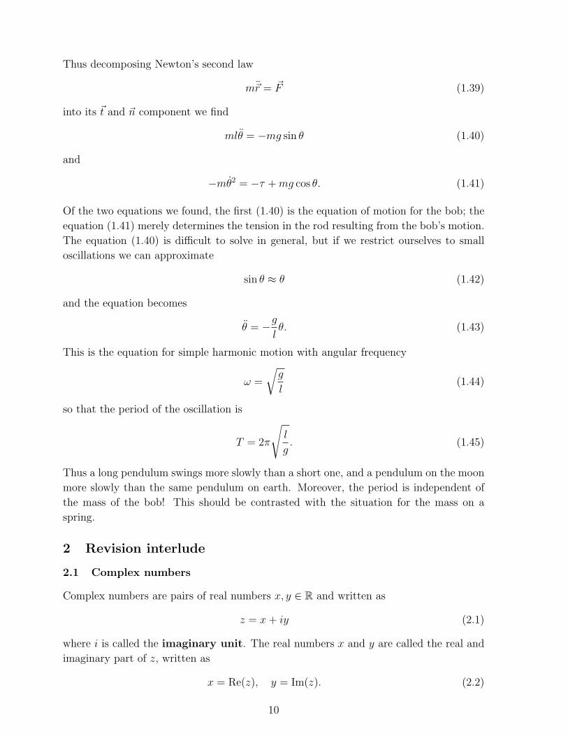
Thus decomposing Newton’s second law

m~r = ~F (1.39)

into its ~t and ~n component we find

mlθ = −mg sin θ (1.40)

and

−mθ2 = −τ + mg cos θ. (1.41)

Of the two equations we found, the first (1.40) is the equation of motion for the bob; the

equation (1.41) merely determines the tension in the rod resulting from the bob’s motion.

The equation (1.40) is difficult to solve in general, but if we restrict ourselves to small

oscillations we can approximate

sin θ ≈ θ (1.42)

and the equation becomes

θ = −g

lθ. (1.43)

This is the equation for simple harmonic motion with angular frequency

ω =

√g

l(1.44)

so that the period of the oscillation is

T = 2π

√l

g. (1.45)

Thus a long pendulum swings more slowly than a short one, and a pendulum on the moon

more slowly than the same pendulum on earth. Moreover, the period is independent of

the mass of the bob! This should be contrasted with the situation for the mass on a

spring.

2 Revision interlude

2.1 Complex numbers

Complex numbers are pairs of real numbers x, y ∈ R and written as

z = x + iy (2.1)

where i is called the imaginary unit. The real numbers x and y are called the real and

imaginary part of z, written as

x = Re(z), y = Im(z). (2.2)

10

The set of all complex numbers is denoted C. Addition of complex numbers is defined

component-wise. If z1 = x1 + iy1 and z2 = x2 + iy2 then

z1 + z2 = x1 + x2 + i(y1 + y2). (2.3)

The multiplication rule is determined once we fix

i2 = −1. (2.4)

Then

z1z2 = x1x2 − y1y2 + i(x1y2 + x2y1). (2.5)

The complex conjugate z of the complex number z is defined as

z = x− iy (2.6)

and satisfies

zz = x2 + y2. (2.7)

It follows that the inverse of z is

1

z=

z

zz=

x− iy

x2 + y2. (2.8)

φ

R

z

y

x

Im(z)

Re(z)

���������������������������������������������������������������������������������������������������������������������������������������������������������������������������������������������������������������������������������������������������������������������������������������������������������������������������������������������������������������������������������������

���������������������������������������������������������������������������������������������������������������������������������������������������������������������������������������������������������������������������������������������������������������������������������������������������������������������������������������������������������������������������������������

������������������������������������������������������������������������������������������������������������������������������������������������������������������������������������������������������������������������������������������������������������������������������������������������������������������������������������������������������������������������������������������������������������������������������������������������

������������������������������������������������������������������������������������������������������������������������������������������������������������������������������������������������������������������������������������������������������������������������������������������������������������������������������������������������������������������������������������������������������������������������������������������������

Figure 2.1: The Argand diagram

Complex numbers can be depicted as vectors in the two-dimensional plane, called the

Argand diagram, where the real part is plotted along the x-axis and the imaginary part

along the y-axis. The length R of the vector representing the complex number z is the

called modulus and the angle φ (measured in radians) it makes with the x-axis is called

the argument of z. The angle φ is only defined up to multiples of 2π, but we adopt the

convention that φ lies in the interval (−π, π] (often called the principal value). Thus the

modulus is given by

R =√

x2 + y2 =√

zz (2.9)

11

and the argument φ satisfies

tan φ =y

x. (2.10)

From the figure we find

x = R cos φ, y = R sin φ (2.11)

or

z = R(cos φ + i sin φ). (2.12)

Using the important Euler relation

eiφ = cos φ + i sin φ (2.13)

we have the modulus-argument representation of z:

z = Reiφ. (2.14)

The modulus of z is also sometimes written as |z|, so |z| = R when z is given by (2.14).

The multiplication of complex numbers is particularly simple in the modulus-argument

form. If z1 = R1eiφ1 and z2 = R2e

iφ2 then

z1z2 = R1R2ei(φ1+φ2). (2.15)

The inverse of z in (2.14) is

1

z=

1

Re−iφ (2.16)

and its complex conjugate is

z = Re−iφ. (2.17)

To end, we note an important consequence of the relation (2.13) and its complex conjugate

e−iφ = cos φ− i sin φ. (2.18)

Adding and subtracting (2.13) and (2.18) we find

cos φ =1

2

(eiφ + e−iφ

)and sin φ =

1

2i

(eiφ − e−iφ

). (2.19)

2.2 Second order differential equations with constant coefficients

2.2.1 Homogeneous equations with constant coefficients

Consider

d2x

dt2+ a1

dx

dt+ a0x = 0, (2.20)

12

where a1 and a0 are real constants. We try solutions of the form

x(t) = eλt. (2.21)

Inserting (2.21) into (2.20) leads to

(λ2 + a1λ + a0)eλt = 0. (2.22)

Since eλt is never zero, we deduce that (2.21) is a solution if λ satisfies the equation

λ2 + a1λ + a0 = 0. (2.23)

This is called the characteristic equation of the differential equation (2.20). Its roots

are

λ1 =−a1 +

√a2

1 − 4a0

2and λ2 =

−a1 −√

a21 − 4a0

2(2.24)

Inserting the roots into (2.21) we thus obtain solutions to the differential equation (2.20.

The nature of the solution depends on the roots.

(i) λ1 6= λ2 real. This is the easiest case: x1(t) = eλ1t and x2(t) = eλ2t are independent

solutions: they form a fundamental set of solutions. The general solution is a linear

combination of x1 and x2:

x(t) = Aeλ1t + Beλ2t, (2.25)

with A and B constants.

(ii) λ1 = λ2 real. In that case we obtain only one solution from (2.21), namely x1(t) =

eλ1t. A second independent solution is given by x2(t) = teλ1t, and the general solution is

of the form

x(t) = (A + Bt)eλ1t (2.26)

(iii) λ1, λ2 complex. In that case λ2 = λ1, so if λ1 = p + iq then λ2 = p − iq. The

functions eλ1t and eλ2t are independent solutions of (2.20) but are complex. To obtain

real solutions we take the linear combinations

x1(t) =1

2(e(p+iq)t + e(p−iq)t) = ept cos(qt)

x2(t) =1

2i(e(p+iq)t − e(p−iq)t) = ept sin(qt) (2.27)

and obtain a real fundamental set. The general solution is of the form

x(t) = ept(A cos(qt) + B sin(qt)). (2.28)

13

roots fundamental set of solutions

λ1 6= λ2 real u1(t) = eλ1t, u2(t) = eλ2t

λ1 = λ2 real u1(t) = eλ1t, u2(t) = teλ1t

λ1 = p + iq, λ2 = p− iq u1(t) = ept cos(qt), u2(t) = ept sin(qt)

Table 1: fundamental sets for constant coefficient equations

2.2.2 Inhomogeneous equations

Consider now

d2x

dt2+ a1

dx

dt+ a0x = f, (2.29)

where f is some function of t.

In order to find all solutions of (2.29) we require

1. A fundamental set {x1, x2} of solutions ofd2x

dt2+ a1

dx

dt+ a0x = 0.

2. A particular solution xp of (2.29).

The general solution is then given by

x = Ax1 + Bx2 + xp, (2.30)

where A and B are real constants.

If the function f in (2.29) is a polynomial, exp, sin or cos, then one can find a particular

solution of a similar form via the method undetermined coefficients. The following

table gives recipes involving unknown coefficients which one can determine by substituting

into the equation. There is no deep reason for these recipes other than that they work.

In the table I have abbreviated homogeneous equation by HE.

14

f(t) particular solution

b0 + b1t + ...bntn c0 + c1t + ...cnt

n

eλt eλt is not a solution of HE ⇒ try ceλt

eλt is a solution of HE ⇒ try cteλt

eλt and teλt solutions of HE ⇒ try ct2eλt

eiωt eiωt not solution of the HE⇒ try Ceiωt , C ∈ C, and take real part

eiωt solution of the HE⇒ try Cteiωt , C ∈ C, and take real part

cos(ωt) Find particular solution for equation with f(t) = eiωt

and take real part

Table 2

To illustrate the recipes given in the table, we consider some examples, beginning with

the polynomial case.

d2x

dt2+ x = t2. (2.31)

We try

xp(t) = b0 + b1t + b2t2, (2.32)

and find by inserting into (2.31)

(2b2 + b0) + b1t + b2t2 = t2 (2.33)

Comparing coefficients yields

b2 = 1, b1 = 0, b0 = −2 (2.34)

so that

xp(t) = t2 − 2. (2.35)

Continuing with the exponential case, consider

d2x

dt2+ 3

dx

dt+ 2x = e3t (2.36)

15

The roots of the characteristic polynomial are −1 and −2. Thus the right hand side is

not a solution of the homogeneous equation, and we try

xp(t) = ce3t (2.37)

and deduce from inserting into (2.36) that xp is a solution provided we choose c = 1/20.

Now change the right hand side of (2.36) to a solution of the homogeneous equation, say

d2x

dt2+ 3

dx

dt+ 2x = e−t. (2.38)

Now we try

xp(t) = cte−t. (2.39)

After slightly tedious differentiations, you should find that this is indeed a solution pro-

vided we pick c = 1.

Finally we turn to the oscillatory case f(t) = cos(ωt). It is particularly important for

applications and we will study it in detail in Sect. 3. According to method summarised

given in the last row of table 2 we should solve the equation with cos(ωt) replaced by eiωt,

and take the real part at the end. The method can be justfied as follows. Suppose x(t) is

a solution of

x + a1x + a0x = eiωt, (2.40)

with a1, a0 and ω all real. Then, taking real parts,

Re (x + a1x + a0x) = Re(eiωt

)= cos(ωt) (2.41)

so, with xp = Re(x), we have Re(x) = xp, Re(a1x) = a1xp and Re(a0x) = a0xp. Hence

xp + a1xp + a0xp = cos(ωt) (2.42)

To illustrated the method, we study one example here:

d2x

dt2+ 3

dx

dt+ 2x = cos(2t). (2.43)

We consider the associated complex equation

d2x

dt2+ 3

dx

dt+ 2x = e2it. (2.44)

Our strategy is to solve this equation, and take the real part of the (complex) solution

as a particular solution for (2.43). Thus we try x(t) = Ce2it with C ∈ C. Differentiating

and inserting into (2.44) we find

(−4C + 6iC + 2C)e2it = e2it (2.45)

16

so that

C =1

−2 + 6i= − 1

20− 3

20i. (2.46)

Thus the particular solution is

xp(t) = Re

((− 1

20− 3

20i

)(cos(2t) + i sin(2t))

)= − 1

20cos(2t) +

3

20sin(2t). (2.47)

17

3 Damped and forced oscillations

3.1 The oscillating spring revisited

Consider a spring hanging vertically as in 1.4, with an object of mass m attached to it.

We are now going to consider the more complicated situation where the object is acted

on by an additional force f(t), and we are going to take friction into account.

The forces acting on the object are

1. The downward gravitational force: mg.

2. The elastic restoring force −k(l + x).

3. Air resistance. This is an example of a damping force which is proportional to the

velocity but acts in the opposite direction: −r dxdt

.

4. Any other force exerted on the object, denoted f(t).

Note that the damping coefficient r has units N · s/m and the spring constant k has units

N/m.

According to Newton’s second law, the motion of the object is thus governed by the

equation

md2x

dt2= mg − k(l + x)− r

dx

dt+ f(t). (3.1)

Re-arranging the terms, and using (1.27) we thus arrive at the linear second-order inho-

mogeneous ODE

md2x

dt2+ r

dx

dt+ kx = f(t). (3.2)

This is the sort of equation which we have learnt to solve in the previous subsection.

Here we will see how to interpret our solutions physically. I have summarised the physical

meaning of the various parameters and functions in the following table.

18

x(t) downward displacement from equilibrium at time t

x(t) velocity at time t

x(t) acceleration at time t

f(t) external or driving force at time t

m mass

r damping coefficient

k spring constant

Table 3

We are now going to study the equation (3.2), starting with the simplest situation and

building up towards the general form (3.2). First consider the case where the damping

constant r is zero, and no additional force f acts on the mass. The equation (3.2) thus

becomes

d2x

dt2+

k

mx = 0. (3.3)

This is the equation of simple harmonic motion we studied at the beginning of the

course. Let’s derive the solution using the general technique developed in subsection 2.2.

The characteristic equation is

λ2 +k

m= 0. (3.4)

With the abbreviation

ω0 =

√k

m(3.5)

a fundamental set of solutions is given by

x1(t) = cos(ω0t), x2(t) = sin(ω0t). (3.6)

The general solution is therefore

x(t) = A cos(ω0t) + B sin(ω0t) (3.7)

in agreement with (1.6).

19

3.2 Unforced oscillations with damping

There is no external force, but the damping coefficient r is not zero. The equation is

md2x

dt2+ r

dx

dt+ kx = 0 (3.8)

or

d2x

dt2+ γ

dx

dt+ ω2

0x = 0 (3.9)

with the abbreviations

γ =r

m(3.10)

and ω0 as in (3.5). The characteristic equation is

λ2 + γλ + ω20 = 0 (3.11)

with roots

λ1 = −γ

2+

√γ2

4− ω2

0 and λ2 = −γ

2−

√γ2

4− ω2

0 (3.12)

Provided the roots are different, a fundamental set is therefore given by

u1(t) = eλ1t , u2(t) = eλ2t. (3.13)

Both physically and mathematically the discussion of the general solution is best organised

according to the sign of γ2 − 4ω20.

(i)Underdamped case: γ2 < 4ω20

We introduce the abbreviation

β =

√ω2

0 −γ2

4(3.14)

so that λ1 = −γ/2 + iβ and λ2 = −γ/2 − iβ. Comparing with table 1 in section 2.5 we

deduce that a real fundamental set is given by

x1(t) = e−γ2t cos(βt) x2(t) = e−

γ2t sin(βt). (3.15)

The general solution is therefore given by

x(t) = e−γ2t(A cos(βt) + B sin(βt)) = R e−

γ2t cos(βt− φ) (3.16)

with R and φ defined as after Eq. (1.6).

The solution still oscillates and has infinitely many zeroes, but the amplitude of the

oscillation decreases exponentially with time. For t → ∞ all solutions tend to zero: the

oscillation dies down.

20

–0.4

–0.2

0

0.2

0.4

0.6

0.8

1

1 2 3 4 5 6 7 8t

Figure 3.1: Plot of the underdamped solution (3.16) for A = 1, B = 0.25, β = 4, γ = 2

0.2

0.4

0.6

0.8

1

0 1 2 3 4 5 6 7 8t

Figure 3.2: The overdamped solution (3.17) for A = 1.5, B = −0.5, λ1 = −0.5, λ2 = −1.5

(ii)Overdamped case: γ2 > 4ω20

In this case both roots λ1 and λ2 (3.12) are real and negative. The general solution is

x(t) = Aeλ1t + Beλ2t. (3.17)

Solutions are zero for at most one value of t (provided A and B do not both vanish) and

tend to 0 for t →∞.

(iii)Critically damped case: γ2 = 4ω20

In this case λ1 = λ2 = −γ/2 and (compare sect. 2.4.3) the general solution is

x(t) = (A + Bt)e−γ2t (3.18)

Again solutions are zero for at most one value of t (provided A and B do not both vanish)

and tend to 0 for t →∞.

The terminology “underdamped”, “overdamped” and “critically damped” has its ori-

gin in engineering applications. The theory developed here applies, for example, to the

springs that provide the damping in cars. When perturbed from equilibrium, under-

damped springs return to the equilibrium position quickly but overshoot. Overdamped

springs take a long time to return to equilibrium. In the critically damped case the

21

0

0.2

0.4

0.6

0.8

1

2 4 6 8 10t

Figure 3.3: Plot of the critically damped solution (3.18) for A = B = 1, γ = 2

spring returns to the equilibrium position very quickly but avoids overshooting. Thus the

critically damped case provides the most efficient damping.

Example 3.2.1 An object of mass m = 2 kg is attached to a spring with spring constant

k = 4 N m−1 and immersed in a viscous liquid with damping constant r = 6 N m−1 s. At

time t = the object is raised 1 m and given an initial downward velocity of 3 m s−1. Find

the subsequent motion of the object.

The equation of motion is

x + 3x + 2x = 0. (3.19)

The characteristic equation has the two real roots λ1 = −2 and λ2 = −1, so the general

solution is

x(t) = Ae−t + Be−2t (3.20)

Since x(0) = A + B = −1 and x(0) = −A− 2B = 3 we deduce A = 1 and B = −2. The

solution

x(t) = e−t − 2e−2t (3.21)

passes through the equilibrium x = 0 once at t = ln 2 s.

3.3 Forced oscillations with damping

This is the most general case, with all terms in eq. (3.2) playing a role. If the external

force f grows indefinitely, it is clear that the spring will eventually break. Remarkably

this can also happen when f is a periodic function which averages to zero. Since this case

is particularly important in applications, we focus on it here. Suppose therefore that

f(t) = f0 cos(ωt), (3.22)

22

where f0 is some constant (in units of Newtons). Then the equation of motion is

md2x

dt2+ r

dx

dt+ kx = f0 cos(ωt). (3.23)

After dividing by m the equation takes the form

d2x

dt2+ γ

dx

dt+ ω2

0x =f0

mcos(ωt). (3.24)

The quickest way to solve this is to use complex numbers. Since cos ωt is the real part of

exp(iωt) we solve

d2x

dt2+ γ

dx

dt+ ω2

0x =f0

meiωt. (3.25)

first and then take the real part of the solution we obtain. This turns out to be an efficient

method. Suppose first that iω is not a solution of the characteristic equation. Then try

x(t) = C exp(iωt). Inserting into (3.25) yields

Ceiωt(−ω2 + iγω + ω20) =

f0

meiωt. (3.26)

Dividing by exp(iωt) and solving for C we find

C =(f0/m)

−ω2 + iγω + ω20

=(f0/m)e−iφ√

(ω20 − ω2)2 + γ2ω2

(3.27)

where

tan φ =γω

ω20 − ω2

(3.28)

Taking the real part of x(t) = C exp(iωt) we therefore find the solution

xp(t) =(f0/m)√

(ω20 − ω2)2 + γ2ω2

cos(ωt− φ). (3.29)

The function

R(ω) =(f0/m)√

(ω20 − ω2)2 + γ2ω2

(3.30)

gives the ω-dependent amplitude of the forced motion. For later use we write it as

R(ω) =f0

mω0ω

1√(ω0

ω− ω

ω0

)2

+ γ2

ω20

(3.31)

The general solution of (3.24) is a linear combination of the particular solution (3.29) and

the fundamental solutions of the free damped system discussed in sect. 2.6.2. Let us for

23

definiteness consider the underdamped case γ2 < 4ω20. Then the relevant fundamental set

is (3.15) and the general solution of the inhomogeneous equation (3.24) is

x(t) = e−γ2t(A cos(βt) + B sin(βt))︸ ︷︷ ︸transient solution

+ xp(t)︸︷︷︸steady state solution

, (3.32)

with α and β as defined in (3.14). The first part is called the transient solution because

it tends to zero for t → ∞. After a long time the solution is dominated by the steady

state solution. Note that this has the same frequency as the driving term (3.22). Also

note that the amplitude of the steady state solution depends on the frequency ω and is

very large when ω = ω0. This phenomenon is called resonance.

Resonance occurs when the driving frequency is equalto the characteristic frequency of the spring.

Depending on the value of r, m and ω the amplitude of the steady state solution at

resonance could be much bigger than the amplitude of the driving force. Finally note

that at resonance tan φ = ∞ so that φ = π/2. Thus the steady solution lags behind

the driving force by π/2 at the resonance frequency. Resonance manifests itself more

dramatically when the damping is small or zero, as we shall see in the next section.

0.2

0.4

0.6

0.8

1

0 1 2 3 4 5 6 7 8omega

Figure 3.4: The amplitude (3.30) for f0 = 2, ω0 = 2, γ = 1

The amplitude of displacement is not maximal at resonance. We now show that the

amplitude of the velocity is maximal there. Differentiating (3.29) we have

xp(r) = −ωR(ω) sin(ωt− φ). (3.33)

This is an oscillation with amplitude

V (ω) = ωR(ω) =f0

mω0

1√(ω0

ω− ω

ω0

)2

+ γ2

ω20

(3.34)

where we used the expression (3.31). Written in this way it is obvious the denominator

is minimal as a function of ω when ω = ω0. Hence the velocity amplitude V is maximal

at resonance.

24

0

0.5

1

1.5

2

1 2 3 4 5 6 7 8omega

Figure 3.5: The velocity amplitude (3.34) for f0 = 2, ω0 = 2, γ = 1

3.4 Forced oscillations without damping

In the absence of damping, the equation (3.23) simplifies to

md2x

dt2+ kx = f0 cos(ωt). (3.35)

This is a special case of the discussion of oscillatory driving terms in sect. 2.5.1. First

consider the case ω 6= ω0, i.e. iω is not a root of the characteristic equation. Then we

have the particular solution

xp(t) =(f0/m)

(ω20 − ω2)

cos(ωt) (3.36)

and therefore the general solution is

x(t) = A cos(ω0t) + B sin(ω0t) +f0/m

(ω20 − ω2)

cos(ωt) (3.37)

which is a fairly complicated superposition of oscillations of different frequencies. It

remains bounded as t →∞.

Next consider the case of resonance. The driving frequency equals the spring’s character-

istic frequency, i.e.

ω = ω0. (3.38)

Again we think of cos(ωt) as the real part of exp(iωt) and study

d2x

dt2+ ω2x = eiωt (3.39)

Since iω is a solution of the characteristic equation, we try x(t) = Ct exp(iωt) in accor-

dance with Table 2. We find

2iωCeiωt = eiωt (3.40)

25

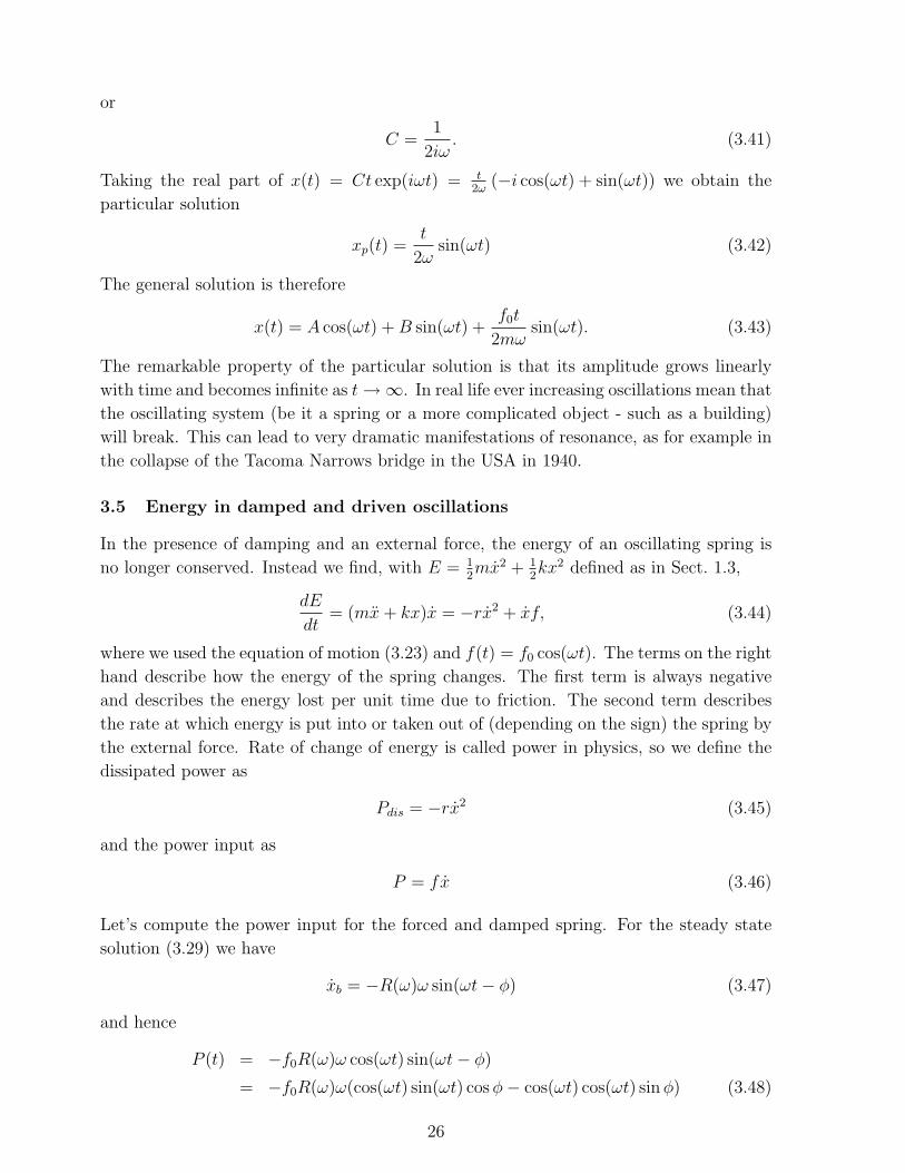
or

C =1

2iω. (3.41)

Taking the real part of x(t) = Ct exp(iωt) = t2ω

(−i cos(ωt) + sin(ωt)) we obtain the

particular solution

xp(t) =t

2ωsin(ωt) (3.42)

The general solution is therefore

x(t) = A cos(ωt) + B sin(ωt) +f0t

2mωsin(ωt). (3.43)

The remarkable property of the particular solution is that its amplitude grows linearly

with time and becomes infinite as t →∞. In real life ever increasing oscillations mean that

the oscillating system (be it a spring or a more complicated object - such as a building)

will break. This can lead to very dramatic manifestations of resonance, as for example in

the collapse of the Tacoma Narrows bridge in the USA in 1940.

3.5 Energy in damped and driven oscillations

In the presence of damping and an external force, the energy of an oscillating spring is

no longer conserved. Instead we find, with E = 12mx2 + 1

2kx2 defined as in Sect. 1.3,

dE

dt= (mx + kx)x = −rx2 + xf, (3.44)

where we used the equation of motion (3.23) and f(t) = f0 cos(ωt). The terms on the right

hand describe how the energy of the spring changes. The first term is always negative

and describes the energy lost per unit time due to friction. The second term describes

the rate at which energy is put into or taken out of (depending on the sign) the spring by

the external force. Rate of change of energy is called power in physics, so we define the

dissipated power as

Pdis = −rx2 (3.45)

and the power input as

P = fx (3.46)

Let’s compute the power input for the forced and damped spring. For the steady state

solution (3.29) we have

xb = −R(ω)ω sin(ωt− φ) (3.47)

and hence

P (t) = −f0R(ω)ω cos(ωt) sin(ωt− φ)

= −f0R(ω)ω(cos(ωt) sin(ωt) cos φ− cos(ωt) cos(ωt) sin φ) (3.48)

26

Using cos(ωt) sin(ωt) = 12sin(2ωt) and

1

T

∫ T

0

sin(2ωt)dt = 0 (3.49)

as well as

1

T

∫ T

0

cos2(ωt)dt =1

2(3.50)

(see (1.24)) we find that the average power input over one cycle is

P =1

T

∫ T

0

P (t)dt =1

2f0ωR(ω) sin φ (3.51)

With the expression

R(ω) =f0

mω0ω

1√(ω0

ω− ω

ω0

)2

+ γ2

ω20

(3.52)

(see (3.31)) for R and

sin φ =γω√

(ω20 − ω2)2 + γ2ω2

=γ

ω0

1√(ω0

ω− ω

ω0

)2

+ γ2

ω20

(3.53)

we have

P =γf 2

0

2mω20

1(ω0

ω− ω

ω0

)2

+ γ2

ω20

(3.54)

Comparing with (3.34) we see that P , like the velocity amplitude V (ω), is maximal when

ω = ω0.

27

4 Coupled oscillators

4.1 Coupled springs

21 xx

mm

kKk

Figure 4.1: Coupled springs

Consider two particles, both of mass m, connected by a spring of spring constant K as

shown in the figure. The particles lie on a horizontal plane and are connected to walls by

springs with spring constant k. Their motion is restricted to a line containing all three

springs. The force on each particle is obtained by applying Hooke’s law to the two springs

connected to the particle. Counting displacement of the particles to the right as positive,

the force exerted by the spring to the left of particle 1 on particle 1 is −kx1. The middle

spring is stretched by an amount (x2 − x1) when the the particles are in the position

shown in the figure. It will therefore exert a force −K(x1 − x2) on particle 1 and a force

−K(x2−x1) on particle 2. Finally the spring on the right exerts a force −kx2 on particle

2. Hence, by Newton’s second law we have the equations of motion

mx1 = −kx1 −K(x1 − x2)

mx2 = −kx2 −K(x2 − x1). (4.1)

This is a system of coupled, linear second order differential equations which looks difficult

to solve. However, if we add the equations we obtain

m(x1 + x2) = −k(x1 + x2) (4.2)

and when we subtract them we get

m(x1 − x2) = −k(x1 − x2)− 2K(x1 − x2). (4.3)

Hence, with abbreviations

y1 = x1 + x2, y2 = x1 − x2 (4.4)

and

ω21 =

k

m, ω2

2 =k

m+ 2

K

m(4.5)

28

we have two decoupled equations

y1 = −ω21y1

y2 = −ω22y2. (4.6)

Each of them is just the equation for simple harmonic motion discussed in Sect. 1. Hence

the general solution is

y1(t) = A1 cos(ω1t) + B1 sin(ω1t)

y2(t) = A2 cos(ω2t) + B2 sin(ω2t) (4.7)

where A1, B1, A2, B2 are arbitrary real constants. Having solved the equation (4.6) in

terms of the coordinates y1 and y2 we recover the general solution x1 and x2 of (4.1) via

x1(t) =1

2(y1(t) + y2(t))

x2(t) =1

2(y1(t)− y2(t)). (4.8)

The coordinates y1 and y2 are called normal mode coordinates, or simply normal modes

of the coupled springs. To understand their physical interpretation, consider the motion

when only one of them is non-vanishing.

1. Assume that y2 = 0 (i.e. A2 = B2 = 0 in (4.7)), and consider the motion of the

particles according to (4.8) when y1 6= 0 . Since x1 = x2 in this case, the two

particles oscillate “in tandem”. The spring in the middle remains unstretched since

x1 − x2 = 0.

2. Assume that y1 = 0 (i.e. A1 = B1 = 0 in (4.7)), and consider the motion of the

particles according to (4.8) when y2 6= 0 . Since x1 = −x2 in this case, the two

particles oscillate “in opposition”. The spring in the middle gets stretched and

compressed in every cycle of the motion.

Since ω1 < ω2, the period T1 = 2π/ω1 of the mode y1 is larger than the period T2 = 2π/ω2

of y2. The normal mode y1 is therefore sometimes called the slow mode, and y2 the fast

mode.

The following example illustrates how normal modes can be used to solve initial value

problems.

Example 4.1.1 Two particles of mass m = 1 kg are connected to springs as shown in

Fig. (4.1). The spring constant of the outer springs is k = 25 N/m and the spring constant

of the middle spring is K = 11/2 N/m . Particle 1 is initially displaced 1 m to the right

and released from rest; particle 2 is initially at rest and at the equilibrium position. Find

the subsequent motion of both particles.

29

We solve this problem in three steps.

Step 1: Translate the initial values into intial values for the normal modes y1 and y2.

From the question we know that x1(0) = 1, x1(0) = 0 and x2(0) = 0, x2(0) = 0. Hence

the initial values for the normal coordinates are

y1(0) = x1(0) + x2(0) = 1, y1(0) = x1(0) + x2(0) = 0

and

y2(0) = x1(0)− x2(0) = 1, y2(0) = x1(0)− x2(0) = 0

Step 2: Solve the initial value problem for the normal modes. With k and K given

in the example, we find from (4.5) that ω1 = 5 s−1 and ω2 = 6 s−1. Hence the general

solution of the normal mode equations (4.6) are y1(t) = A1 cos(5t)+B1 sin(5t) and y2(t) =

A2 cos(6t)+B2 sin(6t). Imposing the initial conditions found in step 1 gives y1(t) = cos(5t)

and y2(t) = cos(6t).

Step3 : Translate the results of step 2 into the particle coordinates x1 and x2. From the

formula (4.8) we find x1(t) = 12(cos(5t) + cos(6t)) and x2(t) = 1

2(cos(5t)− cos(6t)). �

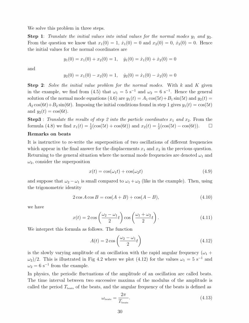
Remarks on beats

It is instructive to re-write the superposition of two oscillations of different frequencies

which appear in the final answer for the displacements x1 and x2 in the previous question.

Returning to the general situation where the normal mode frequencies are denoted ω1 and

ω2, consider the superposition

x(t) = cos(ω1t) + cos(ω2t) (4.9)

and suppose that ω2−ω1 is small compared to ω1 +ω2 (like in the example). Then, using

the trigonometric identity

2 cos A cos B = cos(A + B) + cos(A−B), (4.10)

we have

x(t) = 2 cos

(ω2 − ω1

2t

)cos

(ω1 + ω2

2t

). (4.11)

We interpret this formula as follows. The function

A(t) = 2 cos

(ω2 − ω1

2t

)(4.12)

is the slowly varying amplitude of an oscillation with the rapid angular frequency (ω1 +

ω2)/2. This is illustrated in Fig 4.2 where we plot (4.12) for the values ω1 = 5 s−1 and

ω2 = 6 s−1 from the example.

In physics, the periodic fluctuations of the amplitude of an oscillation are called beats.

The time interval between two successive maxima of the modulus of the amplitude is

called the period Tbeats of the beats, and the angular frequency of the beats is defined as

ωbeats =2π

Tbeats

. (4.13)

30

–2

–1

0

1

2

2 4 6 8 10 12t

Figure 4.2: Beats: plot of cos(5t)+ cos(6t) against t. The dashed curve shows the slowly-varying amplitude ±2 cos(t/2)

The angular frequency of beats which occur in the superposition (4.12) of is twice the

angular frequency of the amplitude oscillation A(t) in (4.12) since the modulus of A(t)

has half the period of A(t) . Thus

ωbeats = ω2 − ω1. (4.14)

Note that Beats are used in tuning instruments. When two notes are slightly out of tune

the difference of their frequencies is small, leading to slow and clearly audible fluctuations

in the amplitude of their combined sound. The notes can be tuned by reducing the

frequency of these beats, ideally to zero.

4.2 N coupled oscillators: beads on a string

Consider N identical beads on a flexible string whose endpoints are connected to walls.

Each bead has a mass m, and we neglect the mass of the string itself. In the equilibrium

position, depicted at the top in Fig. 4.3, the tension in the string is τ and the beads

are separated from each other and the walls by a distance l. The beads are allowed to

move in one transverse direction, and we denote the transverse displacement of the p-th

bead from the equilibrium position by zp, p = 1, . . . , N , see Fig. (4.3). It turns out to

be convenient to introduce the notation z0 and zN+1 for the “displacement” of the points

where the string is connected to the walls. By assumption

z0 = zN+1 = 0. (4.15)

When the beads are displaced from equilibrium the segments of string connecting them are

no longer horizontal. We call the angle between the horizontal and the segment connecting

the p-th and p + 1-st string αp and assume in the following that all these angles are small

αp � 1, p = 1, . . . , N. (4.16)

31

l

N...21

α αα p

p−11

zzz zN

z2

...

...

0 p

p+1

Figure 4.3: N beads on a string

We can therefore use the small angle approximation for trigonometric functions

sin αp ≈ tan αp ≈ αp, p = 1, . . . , N (4.17)

and

cos αp ≈ 1, p = 1, . . . , N. (4.18)

The total force Fp acting on the p-th bead is the difference between the tensions in

the string segments meeting at that bead. Decomposing into horizontal and vertical

components we have from Fig. (4.3)

F horizontal

p = −τ cos αp−1 + τ cos αp. (4.19)

For small angles, it follows from (4.18) that

F horizontal

p ≈ 0. (4.20)

For the vertical component of the force we find, by looking at Fig. (4.3),

F vertical

p = −τ sin αp−1 + τ sin αp. (4.21)

32

Now we express the angles αp in terms of the vertical displacements via

tan αp−1 =zp − zp−1

l, (4.22)

noting that, because of our convention (4.15), this formula holds for all p = 1, . . . , N .

Using the approximation (4.17) we obtain

F vertical

p = −τ

l(zp − zp−1) +

τ

l(zp+1 − zp). (4.23)

Thus, Newton’s second law yields the equations of motion

mzp = −τ

l(zp − zp−1)−

τ

l(zp − zp+1), (4.24)

where p runs from 1 to N . Because of the condition (4.15) the equation for the first and

N -th beads are

mz1 = −τ

lz1 −

τ

l(z1 − z2)

zN = −τ

l(zN − zN−1)−

τ

lzN . (4.25)

In the special case N = 2 of two coupled beads we obtain the coupled equations

z1 = − τ

mlz1 −

τ

ml(z1 − z2)

z2 = − τ

ml(z2 − z1)−

τ

mlz2. (4.26)

With the replacements z1 7→ x1, z2 7→ x2 and τ/(lm) 7→ K/m = k/m, these are the same

equations (4.1) that we found for the coupled springs in the previous section when, in the

notation of Fig 4.1 k = K. Applying our experience gained there we can decouple the

equations by introducing the normal mode coordinates

y1 = z1 + z2, y2 = z1 − z2 (4.27)

and the normal mode angular frequencies ω1 and ω2

ω21 =

τ

ml, ω2

2 =3τ

ml. (4.28)

The equations (4.26) are then equivalent to

y1 = −ω21y1

y2 = −ω22y2 (4.29)

and solved by

y1(t) = A1 cos(ω1t) + B1 sin(ω1t)

y2(t) = A2 cos(ω2t) + B2 sin(ω2t) (4.30)

where A1, B1, A2, B2 are arbitrary real constants.

We can visualise the normal modes as follows. When the beads move in the normal mode

y1 (i.e. y2 = 0) the beads oscillate together. When y1 = 0 and the beads move in the

normal mode y2, they move in opposition: when one is “up” the other is “down” and

vice-versa.

33

4.3 The eigenvector method for finding normal modes

In this subsection we introduce a systematic way of finding normal modes which also

works for N > 2 beads. To motivate it, we re-write the results of the previous section in

matrix form. The inverse of the relation (4.27) is

z1 =1

2(y1 + y2), z2 =

1

2(y1 − y2). (4.31)

Hence, when the beads move in the normal mode y1 given in (4.30) with y2 = 0, the

displacements z1 and z2 at time t can be combined into the two component vector(z1(t)z2(t)

)=

1

2(A1 cos(ω1t) + B1 sin(ω1t))

(11

). (4.32)

When the beads move in the normal mode y2, with y1 = 0, their displacements z1 and z2

at time t are given by(z1(t)z2(t)

)=

1

2(A2 cos(ω2t) + B2 sin(ω2t))

(1−1

). (4.33)

The key property of the vectors (4.32) and (4.33) is that in both cases all components

oscillate with the same frequency. The following method, called the eigenvector method,

takes this as the starting point for finding normal modes. We illustrate how it works using

the example for two beads on a string.

Step 1: Write the equations of motion (4.26) in matrix form:(z1

z2

)= −ω2

0

(2 −1−1 2

) (z1

z2

), (4.34)

where we introduced the abbreviation ω20 = τ/(ml) (Check that this really is the same

equation!)

Step 2: Try to find a non-zero solution of the form(z1(t)z2(t)

)= (A cos(ωt) + B sin(ωt))

(v1

v2

), (4.35)

where ω and A, B, v1, v2 are unknown real constants. Inserting into (4.34) leads to

−ω2((A cos(ωt) + B sin(ωt))

(v1

v2

)= −ω2

0((A cos(ωt) + B sin(ωt))

(2 −1−1 2

) (v1

v2

).(4.36)

Assuming that A and B are not both zero, this can only be true for all t if

−ω2

(v1

v2

)= −ω2

0

(2 −1−1 2

) (v1

v2

), (4.37)

i.e. if (2 −1−1 2

) (v1

v2

)=

ω2

ω20

(v1

v2

). (4.38)

34

Step 3: Solve the matrix equation (4.38). This is an eigenvalue equation for the matrix

M =

(2 −1−1 2

). (4.39)

We need to find its eigenvectors and eigenvalues, i.e. the real numbers ε and vectors v

such that

Mv = εv. (4.40)

In this case it is straightforward to solve the eigenvalue problem - see example sheets.

The matrix M has the eigenvalue ε1 = 1 with eigenvector

v1 =

(11

)(4.41)

and eigenvalue ε2 = 3 with eigenvector

v2 =

(1−1

). (4.42)

Step 4: Obtain a solution of the form (4.35) for every eigenvalue and eigenvector found

in Step 3. Comparing (4.38) and (4.40), we have

ε =ω2

ω20

. (4.43)

Hence ε1 = 1 is equivalent to

ω1 = ω0, (4.44)

and inserting the eigenvector (4.41) into (4.35) we obtain the solution(z1(t)z2(t)

)= (A cos(ω1t) + B sin(ω1t))

(11

). (4.45)

Renaming the arbitrary constants A and B as A1/2 and B1/2 we recover the solution

(4.32). Similarly, from ε2 = 3 we deduce

ω2 =√

3ω0. (4.46)

Inserting the eigenvector (4.42) into (4.35) we obtain the solution(z1(t)z2(t)

)= (A cos(ω2t) + B sin(ω2t))

(1−1

). (4.47)

Renaming the arbitrary constants A and B as A2/2 and B2/2 we recover the solution

(4.33).

35

We end this section by considering the case of an arbitrary number of beads. According

to the eigenvector method, step 1 is to write the equations of motion (4.24) as a matrix

equation: z1

z2...

zN

= −ω20

2 −1 0 0 0−1 2 −1 0 00 −1 2 −1 0

. . .0 0 0 −1 2

z1

z2...

zN

, (4.48)

where we introduced the abbreviation ω20 = τ/(ml). Next, we implement step 2 by

looking for a solution of the formz1(t)z2(t)

...

zN(t)

= (A cos(ωt) + B sin(ωt))

v1

v2...

vN .

(4.49)

Inserting this into (4.48) leads to the eigenvalue problem2 −1 0 0 0−1 2 −1 0 00 −1 2 −1 0

. . .0 0 0 −1 2

v1

v2...

vN

=ω2

ω20

v1

v2...

vN

. (4.50)

Solving this is step 3 in our method. We give the solution in the following lemma. The

proof is left as an exercise on Sheet 9.

Lemma 4.3.1 The matrix

M =

2 −1 0 0 0−1 2 −1 0 00 −1 2 −1 0

. . .0 0 0 −1 2

(4.51)

has N eigenvalues and eigenvectors given by

εn = 2− 2 cos

(nπ

N + 1

), vn =

sin

(nπ

N+1

)sin

(2nπN+1

)...

sin(

NnπN+1

)

(4.52)

where n = 1, . . . , N .

36

0

0.2

0.4

0.6

0.8

1

0 1 2 3 4

–1

–0.5

0

0.5

1

0 1 2 3 4

–1

–0.8

–0.6

–0.4

–0.2

0

0.2

0.4

0.6

0 1 2 3 4

Figure 4.4: Normal modes of three beads on a string

Finally, we carry out step 4 by inserting our results for the eigenvalue problem into

the solution (4.49). Renaming the constants A and B to An and Bn for the solution

corresponding to the n-the eigenvalue εn we obtain N independent solutions. With the

abbreviation

z =

z1

z2...

zN

(4.53)

we have the N solutions

zn(t) = (An cos(ωnt) + Bn sin(ωnt)) vn, (4.54)

where

ω2n = εnω

20. (4.55)

37

The eigenvector method produces N solutions, containing two arbitrary real constants An

and Bn each. The general solution of (4.34) is a linear combination of these. It contains

2N arbitrary constants as we expect for a general solution of a system of second order

differential equation for N functions. The eigenmodes for N = 3 are shown in Fig. 4.4.

Example 4.3.2 Consider the case of N = 3 beads on a string. Each bead has mass

m = 10 gram. If the tension in the string is τ = 1 N and the beads are separated from

each other and the wall by l = 1 m, find the normal modes of the system.

.

With the data given we find ω20 = τ/(ml) = 0.01 s−2, so that ω0 = 0.1 s −1. The angular

frequencies of the three normal modes are given by (4.55) with εn given by (4.52). Inserting

N = 3 and n = 1, 2, 3 we find

ω21 = (2−

√2)ω2

0, ω22 = 2ω2

0, ω23 = (2 +

√2)ω2

0. (4.56)

The normal modes are given by (4.54) with

v1 =

1√2

11√2

, v2 =

10−1

, v3 =

1√2

−11√2

. (4.57)

he displacements of the beads at time t = 0 for each of these normal modes are shown in

Fig. (4.4). �.

38

5 Waves

In this section we derive the wave equation for transverse waves on string. We consider a

string of length L and with a constant mass density µ per unit length stretched between

two walls. We can think of this system as the N →∞ limit of the N beads on a massless

string considered in the previous section. This may sound complicated, but we shall

see in this section that a string with constant mass density is actually easier to describe

mathematically than a finite but large number of beads on a (massless) string.

5.1 The wave equation

Consider the general displacement of the string from equilibrium shown in Fig. (5.1). The

string is allowed to move in one transverse direction (the vertical direction in the figure).

We introduce a coordinate x ∈ [0, L] along the string and denote and the transverse

displacement by z. Since the transverses displacement depends on the time t and on x, z

is a function of t and x. The fact that the string is fixed at its endpoints is mathematically

expressed via

z(t, 0) = z(t, L) = 0, ∀t ∈ R (5.1)

(t,x)

α (t,x ∆

∆z(t,x+ x)

z(t,x)

x)+

xx+ ∆

α

x

Figure 5.1: The stretched string

In order to derive an equation of motion for z, consider a small segment (x, x+∆x) of the

string. The angle between the string and the horizontal is denoted by α; since the angle

varies along the string and also with time, α is a function of t and x. As in the derivation

of the equation of motion for beads on a string we assume that α is small, i.e.

α(t, x) � 1, ∀t ∈ R, x ∈ [0, L], (5.2)

so that

sin α(t, x) ≈ tan α(t, x) ≈ α(t, x), ∀t ∈ R, x ∈ [0, L], (5.3)

and

cos α(t, x) ≈ 1, ∀t ∈ R, x ∈ [0, L]. (5.4)

39

Next we consider the forces acting on the segment (x, x + ∆x). Denoting the tension in

the string by τ , the horizontal force on the segment is

F horizontal(t, x) = −τ cos α(t, x) + τ cos α(t, x + ∆x). (5.5)

However, with the approximation (5.4) we find

F horizontal(t, x) ≈ 0. (5.6)

For the vertical component of the force we find

F vertical(t, x) = −τ sin α(t, x) + τ sin α(t, x + ∆x). (5.7)

Using the approximation (5.3) we simplify the right hand side

sin α(t, x + ∆x)− sin α(t, x) ≈ α(t, x + ∆x)− α(t, x). (5.8)

Furthermore, the Taylor expansion

α(t, x + ∆x) = α(t, x) + ∆x∂α

∂x(t, x) + terms of order(∆x)2 (5.9)

implies, for sufficiently small ∆x,

α(t, x + ∆x)− α(t, x) ≈ ∂α

∂x(t, x)∆x. (5.10)

Hence the vertical component of the force is

F vertical(t, x) ≈ τ∂α

∂x(t, x)∆x. (5.11)

Now we express the angles α(t, x) in terms of the vertical displacements via

tan α(t, x) =z(t, x + ∆x)− z(t, x)

∆x≈ ∂z

∂x, (5.12)

where we have used the Taylor expansion again, and assumed that ∆x is small. For small

angles we therefore have

α(t, x) ≈ ∂z

∂x, (5.13)

so that

F vertical(t, x) ≈ τ∂2z

∂x2(t, x)∆x. (5.14)

In order to derive the equations of motion for the string we apply Newton’s second law

to the string segment [x, x + ∆x]. Recalling that the string has constant mass per unit

length µ, we note that segment [x, x+∆x] has mass µ∆x. We approximate the transverse

40

displacement of that the segment by z(t, x), which becomes exact in the limit ∆x → 0.

Hence the acceleration of the segement is ∂2z∂t2

and we obtain the equation of motion

µ∆x∂2z

∂t2= τ

∂2z

∂x2∆x. (5.15)

Dividing by ∆x we have the partial differential equation

1

v2

∂2z

∂t2=

∂2z

∂x2, (5.16)

where the parameter v is defined in terms of the string tension τ and the mass density µ

v =

√τ

µ. (5.17)

The equation (5.16) is called the wave equation. It is one of the most important equations

of mathematical physics, arising in numerous applications of mathematics to physics.

Before we describe a systematic approach to solving the wave equation in the next section,

we consider a simple solution.

It is easy to check that the function

z(t, x) = cos(ωt) sin(kx) (5.18)

solves the wave equation (5.16) for any pair of real parameters ω and k satisfying

ω = vk. (5.19)

The solution (5.18) is periodic in both space and time. We have already discussed the

periodicity of cos(ωt) in our treatment of simple harmonic motion. Since

cos(ω(t + T )) = cos(ωt) (5.20)

we have the familiar formula for the period

T =2π

ω(5.21)

However, the solution (5.18) is also periodic in space. The equation

sin(k(x + λ)) = sin(kx) (5.22)

holds for all x if we take

λ =2π

k. (5.23)

The parameter λ characterises the spatial periodicity of the wave; it is called the wave-

length.

41

5.2 Standing waves

The solution (5.18) does not, in general, satisfy the boundary condition (5.1) at x = L.

When we require

z(t, L) = 0 ∀t ∈ R (5.24)

we get the extra condition

sin(kL) = 0. (5.25)

This imposes a condition on the allowed values for k. The equation (5.25) holds if

k =nπ

L, n = 1, 2, 3 . . . . (5.26)

We thus obtain n solutions of the wave equation (5.16) satisfying the boundary condition

(5.24):

zn(t, x) = cos(ωnt) sin(nπ

Lx), (5.27)

where

ωn = vnπ

L. (5.28)

In this section we explain a systematic way of obtaining solutions like (5.27). The method

is called separation of variables and is useful in solving many partial differential equa-

tions. The idea is to solve the partial differential equation (5.16) by assuming that the

unkown function z(t, x) is a product of an unknown function g(t) which depends only on

t and an unknown function f(x) which depends only on x. Thus we insert

z(t, x) = g(t)f(x) (5.29)

into (5.16) and hope that we can solve the resulting equations for g and f . It follows from

(5.29) that

∂2z

∂t2(t, x) =

d2g

dt2(t)f(x) (5.30)

and

∂2z

∂x2(t, x) = g(t)

d2f

dx2(x). (5.31)

The insertion of (5.29) into the wave equation leads to

1

v2

d2g

dt2(t)f(x) = g(t)

d2f

dx2(x). (5.32)

Assuming that neither f nor g vanish this is equivalent to

1

v2g(t)

d2g

dt2(t) =

1

f(x)

d2f

dx2(x). (5.33)

42

The left hand side of this equation depends only on t, and the right hand side depends

only on x. The only way two functions of different variables can be identical is if they

are both constants. Assuming for now that the constant is negative, we denote it by −k2.

Thus we obtain two ordinary differential equations, one for the function f which depends

on x

d2f

dx2= −k2f (5.34)

and one for the function g which depends on t only:

d2g

dt2= −v2k2 g. (5.35)

Our assumption (5.29) has thus allowed us to trade one partial differential equation for

two ordinary differential equations with an arbitrary parameter k. Moreover, both equa-

tions are the familiar differential equation for simple harmonic motion. Thus the general

solution of (5.34) is

f(x) = α cos(kx) + β sin(kx) (5.36)

with α, β arbitrary real constants. The condition (5.1) implies

f(0) = 0, f(L) = 0. (5.37)

In order to satisfy f(0) = 0 we must have α = 0. The requirement f(L) = 0 imposes a

condition on k, which we already discussed after (5.25). Thus we conclude that k must

take one of the values

k =nπ

L, n = 1, 2, 3 . . . . (5.38)

Inserting these values into (5.35) we obtain

d2g

dt2= −v2

(nπ

L

)2

g. (5.39)

For each value of n, this is again the equation for simple harmonic motion. So, for each

value of n, we get the general solution

gn(t) = An cos(ωnt) + Bn sin(ωnt) (5.40)

where

ωn = vnπ

L. (5.41)

Finally assembling f and gn into a function of t and x according to (5.29) we obtain the

following solutions of the wave equation and the boundary condition (5.1):

zn(t, x) = (An cos(ωnt) + Bn sin(ωnt)) sin(nπ

Lx)

. (5.42)

43

Here we have set the constant β = 1 in (5.36). This can be done without loss of generality

because β multiplies the the constants An and Bn which are themselves arbitrary.

In analogy to the solutions (4.54) the solutions (5.42) are called the the normal modes of

the string. The mode n = 1

z1(t, x) = (An cos(ω1t) + Bn sin(ω1t)) sin(π

Lx)

. (5.43)

is called the fundamental mode of the string. The solutions for n > 1 are called higher

modes or, in accoustics, overtones. Each mode has a characteristic angular frequency,

period and wavelength. With the angular frequency of the n-th mode given by (5.41), the

period of the n-th mode is

Tn =2π

ωn

=2L

vn. (5.44)

The wavelength can be computed from (5.38) via (5.23). We find

λn =2πnπL

=2L

n. (5.45)

The following example illustrates the importance of normal modes.

Example 5.2.1 Consider a string of length L = 1m, with uniform mass density and

total mass M = 0.1 kg. The string is stretched so that the tension in the string is τ = 10

Newton, and fixed at its endpoints. It is allowed to oscillate freely in one transverse

direction.

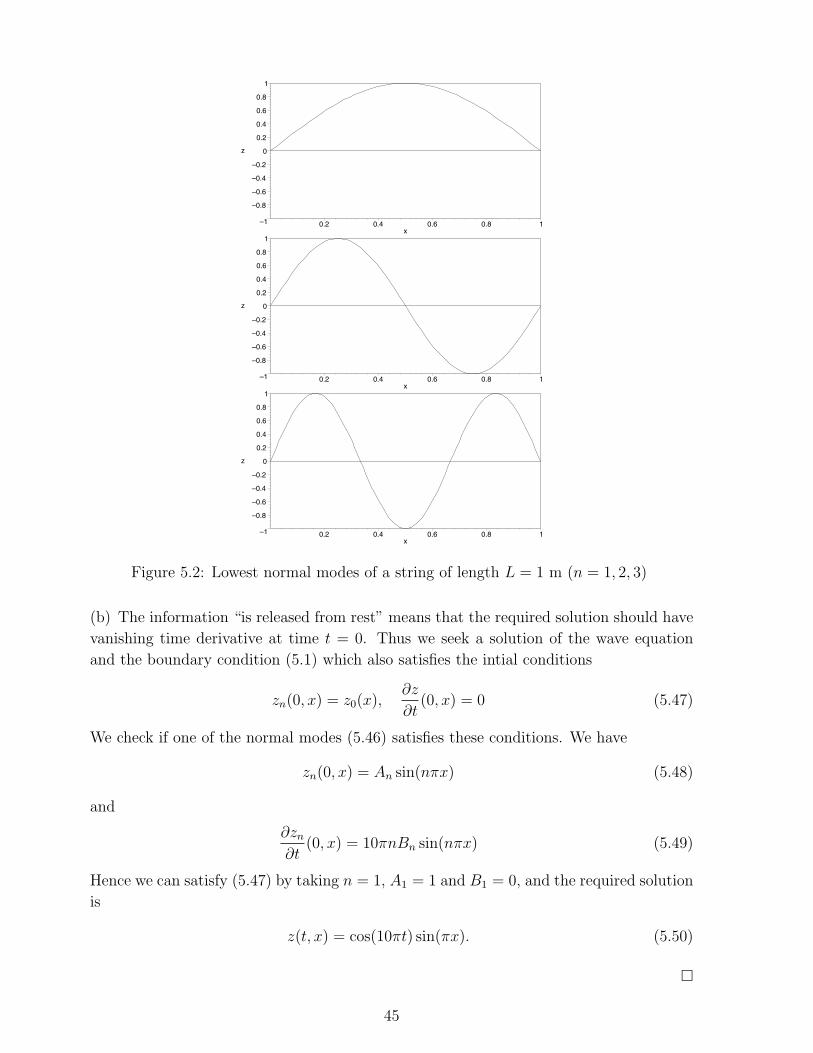
(a) Find all normal modes of the string and give their angular frequencies, periods and

wavelengths. Sketch the lowest three modes at time t = 0.

(b) If the string is given an initial displacement z0(x) = sin(πx) and released from rest,

find its subsequent motion.

(a) The mass density µ is related to the total mass and the length of the string via

µ = M/L. Hence, with the values given in the example, µ = 0.1kg/m. Thus

v =

√τ

µ=√

100m s−1 = 10m s−1.

Inserting the numerical values for v and L into (5.42) we find

zn(t, x) = (An cos(10nπt) + Bn sin(10nπt)) sin(nπx). (5.46)

The angular frequency of the n-th mode is ωn = 10πn s−1, the period is Tn = 15n

s and the

wavelength is λn = 2n

m. The functions zn(0, x) are sketchted for n = 1, 2, 3 in Fig 5.2.

44

–1

–0.8

–0.6

–0.4

–0.2

0

0.2

0.4

0.6

0.8

1

z

0.2 0.4 0.6 0.8 1x

–1

–0.8

–0.6

–0.4

–0.2

0

0.2

0.4

0.6

0.8

1

z

0.2 0.4 0.6 0.8 1x

–1

–0.8

–0.6

–0.4

–0.2

0

0.2

0.4

0.6

0.8

1

z

0.2 0.4 0.6 0.8 1x

Figure 5.2: Lowest normal modes of a string of length L = 1 m (n = 1, 2, 3)

(b) The information “is released from rest” means that the required solution should have

vanishing time derivative at time t = 0. Thus we seek a solution of the wave equation

and the boundary condition (5.1) which also satisfies the intial conditions

zn(0, x) = z0(x),∂z

∂t(0, x) = 0 (5.47)

We check if one of the normal modes (5.46) satisfies these conditions. We have

zn(0, x) = An sin(nπx) (5.48)

and

∂zn

∂t(0, x) = 10πnBn sin(nπx) (5.49)

Hence we can satisfy (5.47) by taking n = 1, A1 = 1 and B1 = 0, and the required solution

is

z(t, x) = cos(10πt) sin(πx). (5.50)

�

45

In the example we were lucky that we could satisfy the initial conditions with one of the

normal modes of the string. For more general initial conditions this will not be possible.

The next section introduces a tool for tackling general intial value problems for the string.

The tool is called Fourier analysis, and widely used in applied mathematics.

5.3 Fourier series

We consider functions on the interval [−L, L], where L > 0, and show that any reasonable

function f : [−L, L] 7→ R can be respresented as a series

f(x) = a0 +∞∑

n=1

an cosnπx

L+

∞∑n=1

bn sinnπx

L(5.51)

with a0, an and bn, n = 1, 2, 3 . . .. We are going to give an explicit formula for these

coefficients further below. To motivate the formula, we recall the definition of an inner

product space, and the expansion of a vector in such a space in an orthognal basis.

Example 5.3.1 The vector space R2 has the inner product

〈(

x1

x2

),

(y1

y2

)〉 = x1y1 + x2y2. (5.52)

(a) Check that the vectors v1 =

(11

)and v2 =

(1−1

)form an orthogonal basis of R2

with respect to the inner product 〈, 〉.

(b) Expand the vector v =

(12

)in the basis {v1, v2}

(a) Using the formula (5.52) we find 〈v1, v2〉 = 1 − 1 = 0 so that v1 and v2 are indeed

orthogonal. They form a basis since any two orthogonal vectors form a basis of the

two-dimensional vector space R2.

(b) We are looking for coefficients c1 and c2 such that

v = c1v2 + c2v2. (5.53)

In order to compute the coefficient c1 , we take the inner product with v1 to find

〈v1, v〉 = c1〈v1, v1〉 (5.54)

and hence

3 = 2c1 ⇒ c1 =3

2. (5.55)

Similarly, to find the coefficient c2 we take the inner product with v2 to find

〈v2, v〉 = c1〈v2, v2〉 (5.56)

46

and hence

−1 = 2c2 ⇒ c2 = −1

2. (5.57)

�

The formulae (5.54) and (5.56) can be summarised in one formla as

cn =〈vn, v〉〈vn, vn〉

n = 1, 2. (5.58)

In this formulation it holds for any vector space with inner product. In order to apply it

to (5.51) we need to consider the space of all functions on [−L, L] as a vector space, and

equip it with an inner product. More precisely, let

H = space of all piecewise continuous functions on[−L, L] (5.59)

and define the inner product of two functions f, g ∈ H as

〈f, g〉 =

∫ L

−L

f(x)g(x)dx. (5.60)

Having defined the vector space H and the inner product we want to expand an arbitray

element of H in a fixed orthogonal set. The set we want to use is

S = {1, cosπx

L, cos

2πx

L, . . . , sin

πx

L, sin

2πx

L, . . .}. (5.61)

Thus we need to show

Lemma 5.3.2 The set S given in (5.61) is an orthogonal set in H.

Proof : The following general results will be useful in the proof. Recall that a function

F : [−L, L] → R is called odd if F (−x) = −F (x) and even if F (−x) = F (x).

1. The integral of any odd function F : [−L, L] → R from −L to L vanishes. i.e.

F (−x) = −F (x) ⇒∫ L

−L

F (x)dx = 0. (5.62)

2. For a non-zero integer N we have∫ L

−L

cosNπx

Ldx = 0 (5.63)

The proof of the first result is an exercise on the example sheets, and the proof of the

second result is an elementary integration. The results allow us to deduce immediately

that the function 1 is orthogonal to all other elements of S:

〈1, sin nπx

L〉 =

∫ L

−L

sinnπx

L= 0 (5.64)

47

since the sine function is odd and, by (5.63),

〈1, cosnπx

L〉 =

∫ L

−L

cosnπx

L= 0. (5.65)

Next consider the inner products

〈cosmπx

L, sin

nπx

L〉 =

∫ L

−L

cosmπx

Lsin

nπx

Ldx. (5.66)

Now use the trigonometric identity 2 sin A cos B = sin(A + B) + sin(A−B) and the fact

that the sine function is odd to deduce

〈cosmπx

L, sin

nπx

L〉 =

1

2

∫ L

−L

sin(m + n)πx

L+ sin

(n−m)πx

Ldx = 0. (5.67)

Using 2 cos A cos B = cos(A + B) + cos(A−B) we find

〈cosmπx

L, cos

nπx

L〉 =

1

2

∫ L

−L

cos(m + n)πx

L+ cos

(n−m)πx

Ldx. (5.68)

Integrating the first terms gives zero by (5.63), and the same holds for the second term

except when n = m. Thus

〈cosmπx

L, cos

nπx

L〉 =

{0 if n 6= mL if n = m.

(5.69)

Finally, using 2 sin A sin B = cos(A−B)− cos(A + B) we find

〈sin mπx

L, sin

nπx

L〉 =

1

2

∫ L

−L

cos(m− n)πx

L− cos

(n + m)πx

Ldx. (5.70)

This time integrating the second terms gives zero by (5.63), but the first term only gives

zero when n 6= m. Thus

〈sin mπx

L, sin

nπx

L〉 =

{0 if n 6= mL if n = m

(5.71)

Hence the set S is an orthogonal set. Moreover we note the inner products of the elements

with themselves

〈1, 1〉 = 2L, 〈sin nπx

L, sin

nπx

L〉 = 〈cos

nπx

L, cos

nπx

L〉 = L (5.72)

�.

The expansion

f(x) = a0 +∞∑

n=1

an cosnπx

L+

∞∑n=1

bn sinnπx

L(5.73)

48

of an element f ∈ H is therefore an expansion in an orthogonal set. Hence we compute

the coefficients a0, an and bn in analogy to (5.58) via

a0 =〈1, f〉〈1, 1〉

=1

2L

∫ L

−L

f(x)dx

an =〈cos nπx

L, f〉

〈cos nπxL

, cos nπxL〉

=1

L

∫ L

−L

f(x) cosnπx

Ldx

bn =〈sin nπx

L, f〉

〈sin nπxL

, sin nπxL〉

=1

L

∫ L

−L

f(x) sinnπx

Ldx (5.74)

The series (5.73) with the coefficients defined by (5.74) is called the Fourier series of f.

Example 5.3.3 Find the Fourier series for f(x) = x, x ∈ [−1, 1]

With L = 1 the formulae (5.74) give

a0 =1

2

∫ 1

−1

xdx = 0 since the integrand is odd

an =

∫ 1

−1

x cosnπx

Ldx = 0 since the integrand is odd

bn =

∫ 1

−1

f(x) sinnπx

Ldx = − 1

nπ[x cos(nπx)]1−1 +

1

nπ

∫ 1

−1

cos(nπx)dx =

= (−1)n+1 2

nπ(5.75)

Hence

f(x) ≈ 2

π[sin(πx)− 1

2sin(2πx) +

1

3sin(3πx) . . . (5.76)

�.

Even though the functions we consider are only defined on the interval [−L, L], the Fourier

series makes sense for all x ∈ R. It converges almost everywhere to a function f which is

a periodic extension of f i.e.

f(x) = f(x− 2nL) for (2n− 1)L < x < (2n + 1)L, n ∈ Z (5.77)

At points x where the function f is not continuous, the Fourier series converges to the

average of the right-limit and the left-limit of f at x.1 This phenomenon is called the

Gibbs phenomenon.

1The right-limit of f at x is defined as limε→0 f(x+ε), with ε > 0 Similarly, the left-limit is limε→0 f(x−ε), with ε > 0.

49

5.4 Using Fourier series for solving the wave equation

In our study of standing waves on a string, the dependence of displacement z on x was

given by a function f on the interval [0, L]. We now show how to obtain a series for such

functions which involves only sine terms (or only cosine terms). The resulting series is

called the half range Fourier series. We start with the Fourier sine series.

Given the function f : [0, L] → R extend it to an odd function f : [−L, L] → R by defining

f(−x) = −f(x). Then the new function f : [−L, L] → R has a (full range) Fourier series

f(x) = a0 +∞∑

n=1

an cosnπx

L+

∞∑n=1

bn sinnπx

L(5.78)

with coefficients defined as in (5.74). However, since f is odd we can use the rule (5.62)

to deduce that a0 = an = 0 in (5.78). Moreover, since both f and sin nπxL

are odd, their

product is even and therefore

bn =1

L

∫ L

−L

f(x) sinnπx

Ldx =

2

L

∫ L

0

f(x) sinnπx

Ldx (5.79)

Thus bn is defined purely in terms of the original function f : [0, L] → R . The series

f(x) =∞∑

n=1

bn sinnπx

L(5.80)

with bn defined via (5.79) is called the Fourier sine series of f : [0, L] → RThe Fourier cosine series of a function f : [0, L] → R is obtained by extending it to

an even function f : [−L, L] → R by defining f(−x) = f(x). Then the new function

f : [−L, L] → R has a full range Fourier series

f(x) = a0 +∞∑

n=1

an cosnπx

L+

∞∑n=1

bn sinnπx

L(5.81)

with coefficients defined as in (5.74). Since f is even we can now use the rule (5.62) to

deduce that bn = 0 in (5.81). Moreover, since both f and cos nπxL

are even, their product

is even, too, and therefore

a0 = =1

2L

∫ L

−L

f(x)dx =1

L

∫ L

0

f(x)dx

an = =1

L

∫ L

−L

f(x) cosnπx

Ldx =

2

L

∫ L

0

f(x) cosnπx

Ldx (5.82)

Thus a0, an are defined purely in terms of the original function f : [0, L] → R . The series

f(x) = a0 +∞∑

n=1

an cosnπx

L(5.83)

with a0, an defined via (5.82) is called the Fourier cosine series of f : [0, L] → R

50

Example 5.4.1 Find the Fourier sine series of the function f(x) = x2, x ∈ [0, π]

From (5.79) we find, with L = π,

bn =2

π

∫ L

0

x2 sin(nx)dx (5.84)

Integrating by parts twice and using sin(nπ) = 0 and cos(nπ) = (−1)n we find

bn = −2π

n(−1)n +

4

πn3(−1)n − 4

πn3. (5.85)

�

Finally, we illustrate the application of Fourier series to initial values problems for the

string.

Example 5.4.2 (a) Find the Fourier sine series of the function f(x) = x(π− x), with

0 < x < π.

(b) Consider a string of length L = π meters, with tension τ = 10 Newton and mass

per unit length µ = 0.1 kg /m. Using the result of (a) find the solution z(t, x) of

the wave equation for the transverse displacement of the string satisfying the initial

conidition

z(0, x) = x(π − x),∂z

∂t(0, x) = 0.

(a) The Fourier sine series on the intervl [0, π] takes the form

f(x) =∞∑

n=1

bn sin(nx), (5.86)

with

bn =2

π

∫ π

0

f(x) sin(nx)dx

=2

π

∫ π

0

x(π − x) sin(nx)dx

=2

π

([−x(π − x)

1

ncos(nx)

]π

0

+1

n

∫ π

0

(π − 2x) cos(nx)dx

)=

2

π

([(π − 2x)

1

n2sin(nx)

]π

0

+2

n2

∫ π

0

sin(nx)dx

)=

4

πn2

[− 1

ncos(nx)

]π

0

=4

πn3(1− (−1)n) (5.87)

so

x(π − x) =∞∑

n=1

4

πn3(1− (−1)n) sin(nx)

≈ 8

π

(sin(x) +

1

27sin(3x) +

1

125sin(5x) . . .

). (5.88)

51

(b) With the parameters given in the question, we find v =√

τ/µ = 10m s−1. Hence,

using the general formula (5.42), the normal modes of the string are those found

already found in (5.46):

zn(t, x) = (An cos(10nt) + Bn sin(10nt)) sin (nx) . (5.89)

It is easy to check (we will do this in the next section) that arbitrary linear combi-

nation of the normal modes also satisfy the wave equation. In particular (ingoring

convergence issues), the infinite sum

z(t, x) =∞∑

n=1

(An cos(10nt) + Bn sin(10nt)) sin (nx) (5.90)

solves the wave equation and satisfies the boundary condition z(t, 0) = z(t, π) = 0.

We now need to choose the constants An and Bn so that the given initial conditions

are also satisfied. Since

∂z

∂t(t, x) =

∞∑n=1

(−10An sin(10nt) + 10Bn cos(10nt)) sin (nx) (5.91)

we have the initial velocity

∂z

∂t(0, x) =

∞∑n=1

10Bn sin (nx) . (5.92)

To make this vanish, we simply choose Bn = 0 for all n. The initial displacement is

z(0, x) =∞∑

n=1

An sin (nx) . (5.93)

We would like this to be equal to x(π − x). Comparing with the sine series (5.88),

we see that we can achieve this by setting

An =4

πn3(1− (−1)n). (5.94)

Hence the required solution of the initial value problem for the vibrating string is

z(t, x) =∞∑

n=1

4

πn3(1− (−1)n) cos(10nt) sin (nx) . (5.95)

52

To end this section, we collect the similarities between eigenvector method for studying

the motion of beads on a string and the separation of variables method for solving the

motion of a string in a table.

N beads on a string Vibrating string

equation of motiond2z

dt2= − τ

mMz

∂2z

∂t2=

τ

µ

∂2z

∂x2

normal mode equation Mvn = εnvn d2fn

dx2= −k2

nfn

eigenvalues εn = 2− 2 cos

(nπ

N + 1

)kn =

nπ

L

normal modes vnj = sin

(njπ

N + 1

)fn(x) = sin

(nxπ

L

)

〈vn, vm〉 =N + 1

2δnm

∫ L

0

fn(x)fm(x)dx =L

2δnm

normal frequencies ω2n =

τ

mεn ω2

n =τ

µk2

n

general solutionN∑

n=1

(An cos(ωnt) + Bn sin(ωnt)) vn

∞∑n=1

(An cos(ωnt) + Bn sin(ωnt)) fn(x)

Table 5: The eigenvector method versus the separation of variables

53

5.5 Travelling waves

In this subsection we return to the wave equation

1

v2

∂2z

∂t2=

∂2z

∂x2, (5.96)

and discuss a class of solutions called travelling waves. So far we have only considered

standing waves of the form

zk(t, x) = cos(ωt) sin(kx). (5.97)

However, using the trigonometric identity 2 cos A sin B = sin(A+B)+ sin(B−A) we can

write this solution as

zk(t, x) =1

2(sin(kx + ωt) + sin(kx− ωt)) . (5.98)

Now it is easy to check that both

zk,+(t, x) = sin(kx + ωt) (5.99)

and

zk,−(t, x) = sin(kx− ωt) (5.100)

satisfy the wave equation (5.96) provided that the relation

ω = vk (5.101)

is satisfied. Note that neither of these solutions satisfy the boundary condition z(t, 0) =

z(t, L) = 0. However, recall that our derivation of the wave equation in Sect. 5.1 was

independent of the boundary condition. Hence we can think of the wave equation without

boundary conditions as a mathematical description of the transverse displacement of an

infinitely long string. This is the point of view we take in this section: the range of x

is all of R, and no boundary conditions are imposed. In particular, we therefore do not

have any conditions on the parameter k: it is an arbitrary real number. We may assume

without loss of generality that k > 0 since changing the sign of k in (5.99) and (5.100) does

not lead to an essentially new solution. Similarly, we assume without loss of generality

that ω > 0.

Both the solution (5.99) and (5.100) are examples of travelling waves. To understand in

what sense they “travel” consider the spatial dependence of, for example, z+ at time time

t = 0:

zk,+(0, x) = sin(kx) (5.102)

A time interval ∆t > 0 later the wave is

zk,+(∆t, x) = sin(kx + ω∆t). (5.103)

54

While (5.102) is a sine function with period T = 2πω

and which vanishes at the origin, the

function (5.103) (viewed as a function of x) , is a sine function with the same period but

shifted to the left by ∆x = ωk∆t. Using (5.101) we have

∆x = v∆t. (5.104)

Since this holds for an arbitrary interval ∆t we can visualise the solution z+ as a wave

which moves to the left with speed v, see Fig. (5.3).

–1

–0.5

0

0.5

1

–1 1 2 3 4 5 6x

Figure 5.3: Left moving wave: plot of sin(2x + t) for t = 0 (solid line) and t = 1 (dashedline)

A similar analysis for z− leads to the conclusion that it is a wave which moves to the right

with speed v, see Fig. (5.4).

–1

–0.5

0

0.5

1

–1 1 2 3 4 5 6x

Figure 5.4: Right moving wave: plot of sin(2x− t) for t = 0 (solid line) and t = 1 (dashedline)

We thus arrive at the remarkable conclusion that the standing wave (5.97) is a sum of

a left- and a right-moving wave. Moreover we found the physical interpretation of the

parameter v: it is the speed of travelling wave solutions of the wave equation (5.96).

It is surprisingly easy to write down infinitely many travelling wave solutions, as shown

by the following theorem.

Theorem 5.5.1 Let f : R → R be an arbitrary twice differentiable function. Then

z+(t, x) = f(x + vt) and z−(t, x) = f(x− vt) both satisfy the wave equation (5.96).

55

Proof: Let u = x + vt. Then

∂z+

∂t=

df

du

∂u

∂t= v

df

du

and∂2z+

∂t2= v2d2f

du2.

Also∂z+

∂x=

df

du

∂u

∂x=

df

du

and∂2z+

∂x2=

d2f

du2.

Hence1

v2

∂2z+

∂t2=

d2f

du2=

∂2z+

∂x2.

Similarly defining w = x− vt, we have

∂z−∂t

=df

dw

∂w

∂t= −v

df

dw

and∂2z−∂t2

= v2 d2f

dw2.

Also∂z−∂x

=df

dw

∂w

∂x=

df

dw

and∂2z−∂x2

=d2f

dw2.

Hence1

v2

∂2z−∂t2

=d2f

dw2=

∂2z−∂x2

.

�

Using this theorem, we can construct waves of arbitrary shape. Taking for example the

Gaussian f(u) = exp(−u2) we can construct a right travelling wave

z−(t, x) = exp(−(x− vt)2)

which, at any time t, looks like a “bell” centered at vt, see Fig 5.5.

We have already seen how to construct a standing wave by adding two travelling waves,

one travelling to the right and one travelling to the left. In fact we can add any two

solutions of the wave equation to obtain another solution. Although this result is easy to

prove (see below), it is of fundamental importance in the study of the wave equation. It

is called the superposition principle. We state in the following form:

Theorem 5.5.2 Suppose z1(t, x) and z2(t, x) satisfy the wave equation (5.96) and A, B

are real constants. Then z(t, x) = Az1(t, x) + Bz2(t, x) also satisfies the wave equation.

56

0

0.2

0.4

0.6

0.8

1

–4 –2 2 4 6x

Figure 5.5: Right moving bell shape: plot of exp(−(x − t)2) for t = 0 (solid line) andt = 1 (dashed line)

Proof: The result follows from the linearity of the wave equation. With z(t, x) as defined

in the theorem we deduce∂z

∂t= A

∂z1

∂t+ B

∂z2

∂t

and∂2z

∂t2= A

∂2z1

∂t2+ B

∂2z2

∂t2.

Similarly∂z

∂x= A

∂z1

∂x+ B

∂z2

∂x

and∂2z

∂x2= A

∂2z1

∂x2+ B

∂2z2

∂x2.

Hence

1

v2

∂2z

∂t2= A

1

v2

∂2z1

∂t2+ B

1

v2

∂2z2

∂t2

= A∂2z1

∂x2+ B

∂2z2

∂x2

=∂2z

∂x2, (5.105)

where we used that both z1 and z2 satisfy the wave equation in the intermediate step. �

57