Module 4: Chapter 6 Bayesian Learning

Module 4: Chapter 6

Bayesian Learning

1. Introduction

• A probabilistic approach to inference

▫ It is based on the assumption that the quantities of interest are governed by probability distributions and that optimal decisions can be made by reasoning about these probabilities together with observed data.

• Quantitative approach to weighing the evidence supporting alternative hypotheses

• Important

▫ Calculates the explicit probability like naïve Bayes.

Naive Bayes classifier competitive, outperforms as a classifier

▫ They help Understand learning algorithms that do not explicitly manipulate probabilities

17-10-2019 Machine Learning-15CS73

4

• Bayesian learning methods are relevant to our study of machine

learning for two different reasons.

i. Bayesian learning algorithms that calculate explicit

probabilities for hypotheses, such as the naive Bayes

classifier, are among the most practical approaches to

certain types of learning problems.


5

For ex : Michie et al.(1994) provide a detailed study

comparing the naive Bayes classifier to other learning

algorithms, including decision tree and neural network

algorithms.

These researchers show that the naive Bayes classifier is

competitive with these other learning algorithms in many

cases and that in some cases it outperforms these other

methods.

ii. The Bayesian methods are important to our study of

machine learning is that they provide a useful perspective

for understanding many learning algorithms that do not

explicitly manipulate probabilities.


6

For ex : We will analyze the algorithms such as the FIND-

S and Candidate-Elimination algorithms to determine the

conditions under which they output the most probable

hypothesis given the training data.

Bayesian analysis provides an opportunity for the

choosing the appropriate alternative error function(cross

entropy) in neural network learning algorithms.

We use a Bayesian perspective to analyze the inductive

bias of decision tree learning algorithms that favor short

decision trees and examine the closely related Minimum

Description Length principle.

Feature of Bayesian learning methods

include: • Each observed training example can incrementally decrease or

increase the estimated probability that a hypothesis is correct. This provides a more flexible approach to the learning compared to the algorithms that completely eliminate a hypothesis if it is found to be inconsistent with any single example.

• Prior knowledge can be combined with observed data to determine the final probability of a hypothesis. The prior probability is got through (i) a prior probability of each candidate hypothesis (ii) a probability distribution over observed data for each possible hypothesis.

• Bayesian methods can accommodate hypotheses that make probabilistic predictions For ex : hypotheses such as “this pneumonia patient has a 93% chance of complete recovery”

• New instances can be classified by combining the

predictions of multiple hypotheses, weighted by their

probabilities.

• Even in cases where Bayesian methods prove

computationally intractable, they can provide a

standard of optimal decision making against which

other practical methods can be measured.

Difficulty of applying Bayesian method

• Bayesian methods typically require initial knowledge of many

probabilities.

• The significant computational cost required to determine the

Bayes optimal hypothesis in the general case.

2. BAYES THEOREM

• Determining the most (best) hypothesis from some space H, (having initial prior probabilities of various hypotheses ) given the observed training data D.

• Calculates the probability of a hypothesis based on its prior probability, the probabilities of observing various data given the hypothesis, and the observed data itself.

Notation

• P(h) : initial probability that hypothesis h holds, before we have observed the training data. prior probability of h and may reflect any background knowledge we have about the chance that h is a correct hypothesis.

• P(D) : prior probability that training data D will be observed-no knowledge of h

• P(D|h) : probability of observing data D in which hypothesis h holds.

• P(h|D) : probability that h holds given the observed training data D. posterior probability of h reflects the influence of the training data D

• The learner considers some set of candidate hypotheses H and is interested in finding the most probable hypothesis h ϵ H given the

observed data D (or at least one of the maximally probable if there are several).

• Any such maximally probable hypothesis is called a maximum a posteriori (MAP) hypothesis

• We can determine the MAP hypotheses by using Bayes theorem to calculate the posterior probability of each candidate hypothesis.

hMAP is a MAP hypothesis provided

• In some cases, we will assume that every hypothesis in H is equally probable a priori (P(hi) = P(hj) for all hi and hj in H).

• In this case we can further simplify Equation and need only consider the term P(D|h) to find the most probable hypothesis

• P(D|h) is often called the likelihood of the data D given h • Any hypothesis that maximizes P(D|h) is called a

maximum likelihood (ML) hypothesis, hML.

Example:

• To illustrate Bayes rule, consider a medical diagnosis problem in which there are two alternative hypotheses:

(1) that the patient has a particular form of cancer

(2) that the patient does not.

• The available data is from a particular laboratory test with two possible outcomes: + (positive) and - (negative).

• We have prior knowledge that over the entire population of people only .008 have this disease.

• Furthermore, the lab test is only an imperfect indicator of the disease.

• The test returns a correct positive result in only 98% of the cases in which the disease is actually present and a correct negative result in only 97% of the cases in which the disease is not present.

• In other cases, the test returns the opposite result.

• Suppose we now observe a new patient for whom the lab test returns a positive result.

• Should we diagnose the patient as having cancer or not?

3. BAYES THEOREM AND CONCEPT

LEARNING

• What is the relationship between Bayes theorem and the problem of concept learning?

▫ Bayes theorem provides a principled way to calculate the

posterior probability of each hypothesis given the training data

▫ we can use it as the basis for a straightforward learning algorithm that calculates the probability for each possible hypothesis

▫ then outputs the most probable.

3.1 Brute-Force Bayes Concept

Learning

• Concept learning problem:

▫ assume the learner considers some finite hypothesis space H

▫ defined over the instance space X,

▫ the task is to learn some target concept c : X -> {0,1}.

▫ learner is given some sequence of training examples ((x1,d1 ). . . (xm, dm))

• We can design a straightforward concept learning algorithm to output the maximum a posteriori hypothesis, based on Bayes theorem.

BRUTE-FORCE MAP LEARNING algorithm

• what values are to be used for P(h) and for P(D|h) ?

▫ choose the probability distributions P(h) and P(D|h) in

any way you wish, to describe our prior knowledge about the learning task.

▫ Here let us choose them to be consistent with the following assumptions:

1. The training data D is noise free (i.e., di = c(xi)).

2. The target concept c is contained in the hypothesis space H

3. We have no a priori reason to believe that any

hypothesis is more probable than any other.

• Given these assumptions, what values should we specify for P(h)?

▫ Given no prior knowledge that one hypothesis is more likely than another, it is reasonable to assign the same prior probability to every hypothesis h in H.

▫ because we assume the target concept is contained in H we should require that these prior probabilities sum to 1.

• Together these constraints imply that we should choose

• What choice shall we make for P(D|h)?

▫ P(D|h) is the probability of observing the target values D = (d1 . . dm) for the fixed set of instances (x1 . . . xm), given a world in which hypothesis h holds (i.e., given a world in which h is the correct description of the target concept c).

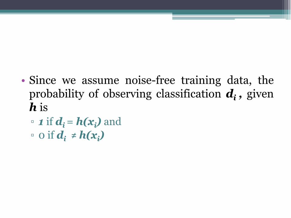
• Since we assume noise-free training data, the probability of observing classification di , given h is

▫ 1 if di = h(xi) and

▫ 0 if di ≠ h(xi)

In other words, the probability of data D given hypothesis h is 1 if D is consistent with h, and 0 otherwise.

• Given these choices for P(h) and for P(D|h) we now have a fully-defined problem for the above BRUTE-FORCE MAP LEARNING algorithm.

• Step1 :

▫ Let us consider the first step of this algorithm, which uses Bayes theorem to compute the posterior probability P(h|D) of each hypothesis h given the observed training data D.

• Case 1 : h is inconsistent with the training data D.

The posterior probability of a hypothesis inconsistent with D is zero.

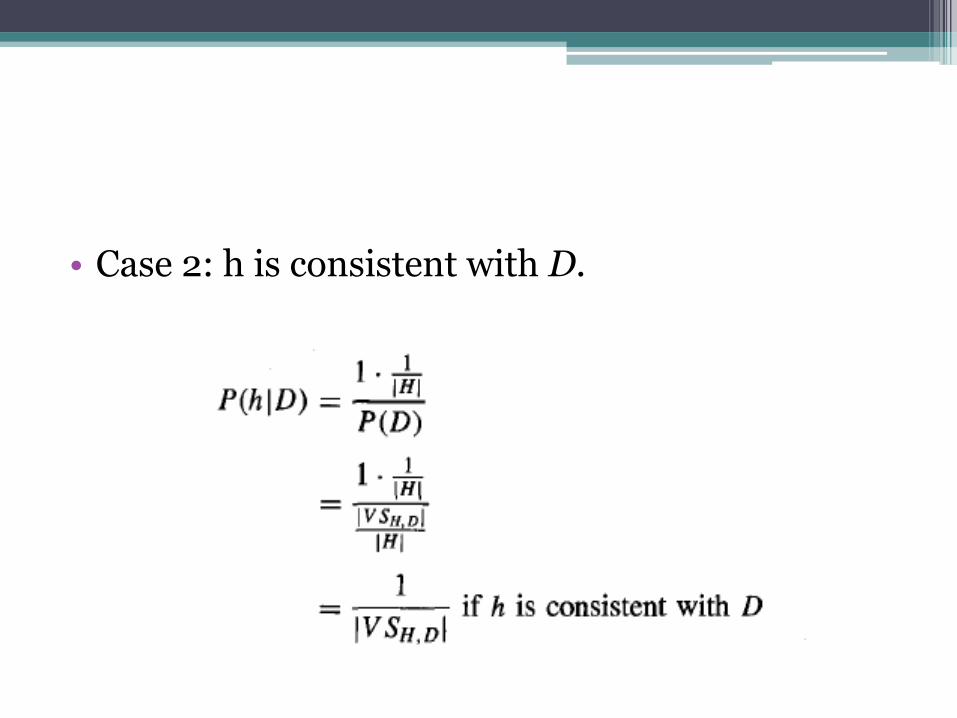
• Case 2: h is consistent with D.

• The above analysis implies that under our choice for P(h) and P(D|h), every consistent hypothesis has posterior probability (1 /|VSH,D| ), and every inconsistent hypothesis has posterior probability 0.

• Every consistent hypothesis is, therefore, a MAP hypothesis.

3.2 MAP Hypotheses and Consistent

Learners

• Every hypothesis consistent with D is a MAP hypothesis

consistent learners:

• We will say that a learning algorithm is a consistent learner provided it outputs a hypothesis that commits zero errors over the training examples.

• Given the above analysis, we can conclude that every consistent learner outputs a MAP hypothesis, if we assume

▫ a uniform prior probability distribution over H (i.e., P(hi) = P(hj) for all i, j), and

▫ deterministic, noise free training data (i.e., P(D|h) = 1 if D and h are consistent, and 0 otherwise).

4. MAXIMUM LIKELIHOOD AND LEAST-

SQUARED ERROR HYPOTHESES

• Let’s we consider the problem of learning a continuous-valued target function.

• A straightforward Bayesian analysis will show that under certain assumptions any learning algorithm that minimizes the squared error between the output hypothesis predictions and the training data will output a maximum likelihood hypothesis.

• Consider the following problem setting:

• Learner L considers an instance space X and a hypothesis space H consisting of some class of real-valued functions defined over X (i.e., each h in H is a function of the form h : X R, where R represents the set of real numbers).

• The problem faced by L is to learn an unknown target function f : X R drawn from H.

• A set of m training examples is provided, where the target value of each example is corrupted by random noise drawn according to a Normal probability distribution.

• More precisely, each training example is a pair of the form (xi, di) where

di = f (xi) + ei

▫ f(xi) : the noise-free value of the target function

▫ ei: is a random variable representing the noise.

• It is assumed that the values of the ei are drawn independently and that they are distributed according to a Normal distribution with zero mean.

• The task of the learner is to output a maximum likelihood hypothesis, or, equivalently, a MAP hypothesis assuming all hypotheses are equally probable a priori.

2 basic concepts

• probability densities

• Normal distributions.

• First, in order to discuss probabilities over continuous variables such as e, we must introduce probability densities.

• The reason, roughly, is that we wish for the total probability over all possible values of the random variable to sum to one.

• In the case of continuous variables we cannot achieve this by assigning a finite probability to each of the infinite set of possible values for the random variable.

• Instead, we speak of a probability density for continuous variables such as e and require that the integral of this probability density over all possible values be one.

• Second, we stated that the random noise variable e is generated by a Normal probability distribution.

• A Normal distribution is a smooth, bell-shaped distribution that can be completely characterized by its mean μ and its standard deviation σ.

• Given this background we now return to the main issue:

▫ showing that the least-squared error hypothesis is, in fact, the maximum likelihood hypothesis within our problem setting.

• We will show this by deriving the maximum likelihood hypothesis, but using lower case p to refer to the probability density

• we assume a fixed set of training instances (x1, x2 . . . xm) and

• Therefore consider the data D to be the corresponding sequence of target values D = ( d1, d2 . . .dm).

• Here di = f (xi) + ei.

• Assuming the training examples are mutually independent given h,

• we can write P(D|h) as the product of the various p(di|h)

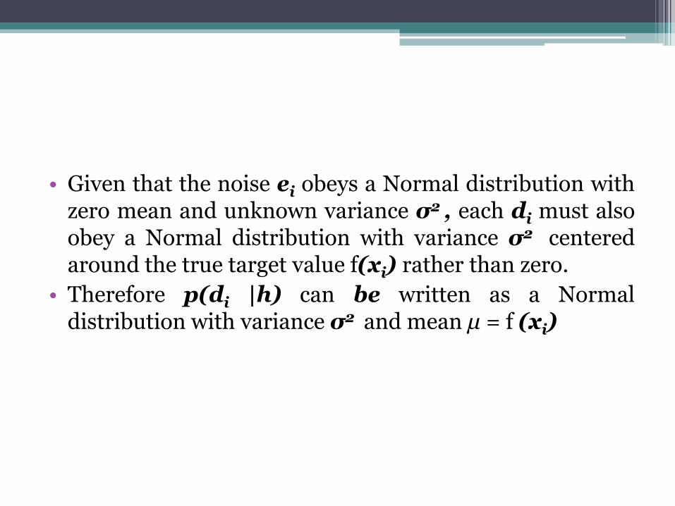
• Given that the noise ei obeys a Normal distribution with zero mean and unknown variance σ2 , each di must also obey a Normal distribution with variance σ2 centered around the true target value f(xi) rather than zero.

• Therefore p(di |h) can be written as a Normal distribution with variance σ2 and mean μ = f (xi)

• Thus, Equation shows that the maximum likelihood hypothesis hML is the one that minimizes the sum of the squared errors between the observed training values di and the hypothesis predictions h(xi).

• Limitations of this problem setting.

▫ The above analysis considers noise only in the target value of the training example and does not consider noise in the attributes describing the instances themselves.

Machine Learning-Module 4

11-11-2019 Machine Learning-15CS73 1


Chapter 6: Bayesian Learning

Introduction

• Bayesian reasoning provides a probabilistic approach to

inference.

• Bayesian learning methods are relevant to our study of machine

learning for two different reasons.

i. Bayesian learning algorithms that calculate explicit

probabilities for hypotheses, such as the naive Bayes

classifier, are among the most practical approaches to

certain types of learning problems.


For ex : Michie et al.(1994) provide a detailed study

comparing the naive Bayes classifier to other learning

algorithms, including decision tree and neural network

algorithms.

These researchers show that the naive Bayes classifier is

competitive with these other learning algorithms in many

cases and that in some cases it outperforms these other

methods.

ii. The Bayesian methods are important to our study of

machine learning is that they provide a useful perspective

for understanding many learning algorithms that do not

explicitly manipulate probabilities.


For ex : We will analyze the algorithms such as the FIND-

S and Candidate-Elimination algorithms to determine the

conditions under which they output the most probable

hypothesis given the training data.

Bayesian analysis provides an opportunity for the

choosing the appropriate alternative error function(cross

entropy) in neural network learning algorithms.

We use a Bayesian perspective to analyze the inductive

bias of decision tree learning algorithms that favor short

decision trees and examine the closely related Minimum

Description Length principle.


Features of Bayesian Learning methods

• Each observed training example can incrementally decrease or

increase the estimated probability that a hypothesis is correct.

This provides a more flexible approach to the learning compared

to the algorithms that completely eliminate a hypothesis if it is

found to be inconsistent with any single example.

• Prior knowledge can be combined with observed data to

determine the final probability of a hypothesis. The prior

probability is got through (i) a prior probability of each candidate

hypothesis (ii) a probability distribution over observed data for

each possible hypothesis.

• Bayesian methods can accommodate hypotheses that make

probabilistic predictions For ex : hypotheses such as “this

pneumonia patient has a 93% chance of complete recovery”


• New instances can be classified by combining the predictions of

multiple hypotheses, weighted by their probabilities.

• Even in cases where Bayesian methods prove computationally

intractable, they can provide a standard of optimal decision making

against which other practical methods can be measured.

Practical Difficulties in applying Bayesian Methods

• Bayesian methods typically require initial knowledge of many

probabilities.

• The significant computational cost required to determine the Bayes

optimal hypothesis in the general case.


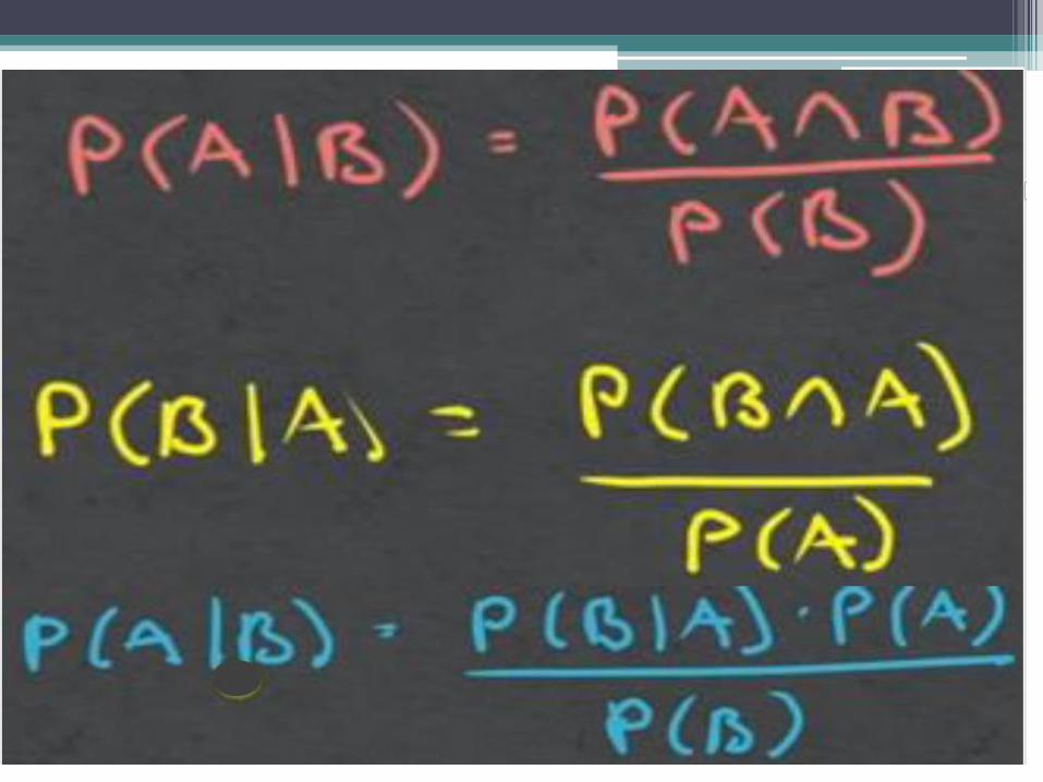
Bayes Theorem

• In machine learning we are interested in determining the best

hypothesis from some space H, given the observed training data D.

• Bayes theorem provides a way to calculate the probability of a

hypothesis based on its prior probability, the probabilities of

observing various data given the hypothesis, and the observed data

itself.

• To define Bayes theorem precisely, let us define the following

notations

P(h) denote the initial probability or prior probability that

hypothesis h holds.

P(D) – denote the prior probability that training data D will be

observed.


P(D/h) denote the probability of observing data D given some

world in which hypothesis h holds.

P(h/D) denote the posterior probability of h because it

reflects our confidence that h holds after we have

seen the training data D.

• Bayes theorem is the cornerstone of Bayesian learning methods

because it provides a way to calculate the posterior probability

P(h/D) from the prior probability P(h), together with P(D) and

P(D/h)

𝑷 𝒉/𝑫 =𝑷 𝑫/𝒉 𝑷(𝒉)

𝑷(𝑫)

• P(h/D) increases with P(h) and with P(D/h) according to Bayes

theorem.

Eqn 6.1


• It is also reasonable to see that P(h/D) decreases as P(D) increases,

because the more probable it is that D will be observed

independent of h, the less evidence D provides in support of h.

• In many learning scenarios, the learner considers some set of

candidate hypotheses H and is interested in finding the most

probable hypothesis hH given the observed data D.

• Any such maximally probable hypothesis is called a maximum a

posteriori (MAP) hypothesis.

• We can determine the MAP hypotheses by using Bayes theorem to

calculate the posterior probability of each candidate hypothesis.

• More precisely, we will say that hMAP is a MAP hypothesis

provided:


• Notice in the final step above we dropped the term P(D) because it

is a constant independent of h.

• In some cases, we will assume that every hypothesis in H is equally

probable a priori (P(hi) = P(hj) for all hi and hj in H). In this case

we can further simplify Eqn 6.2 and need only consider the term

P(D/h) to find the most probable hypothesis.

Eqn 6.2


• P(D/h) is often called the likelihood of the data D given h, and any

hypothesis that maximizes P(D/h) is called a maximum likelihood

(ML) hypothesis, hML

• In order to make clear the connection to machine learning

problems, we have learnt Bayes theorem above by referring to the

data D as training examples of some target function and referring to

H as the space of candidate target functions.

Eqn 6.3


An Example

• To illustrate Bayes rule, consider a medical diagnosis problem in

which there are two alternative hypotheses:

i. that the patient has a particular form of cancer

ii. that the patient does not

• The available data is from a particular laboratory test with two

possible outcomes: ⊕ (positive) and ⊝ (negative).

• We have prior knowledge that over the entire population of people

only .008 have this disease.

• The test returns a correct positive result in only 98% of the cases in

which the disease is actually present and a correct negative result in

only 97% of the cases in which the disease is not present.


• In other cases, the test returns the opposite result.

• The above situation can be summarized by the following

probabilities:

• Suppose we now observe a new patient for whom the lab test

returns a positive result. Should we diagnose the patient as having

cancer or not?

• The maximum a posteriori hypothesis can be found using Eqn 6.2:

P(cancer/⊕) = P(⊕/cancer) P(cancer) = 0.98 * 0.008= 0.0078

P(¬cancer/⊕) = P(⊕/¬cancer) P(¬cancer) = 0.03* 0.992=0.0298


• Thus, hMAP = ¬cancer

• Notice that while the posterior probability of cancer is significantly

higher than its prior probability, the most probable hypothesis is

still that the patient does not have cancer.

• As this example illustrates, the result of Bayesian inference

depends strongly on the prior probabilities, which must be

available in order to apply the method directly.

• Basic formulas for calculating probabilities are summarized in

Table 6.1.


Table 6.1: Summary of basic probability formulas


Bayes Theorem and Concept Learning

• Consider the concept learning problem in which we assume that

learner considers some finite hypothesis space H defined over the

instance space X, in which the task is to learn some target concept

c:X→{0,1}.

• Let us assume that the learner is given some sequence of training

examples <<x1,d1>…<xm,dm>> where xi is some instance from X

and where di is the target value of xi (i.e., di=c(xi)).

• To understand in very simple way, let us make one more

assumption that the sequence of instances <xl . . . xm> is held

fixed, so that the training data D can be written simply as the

sequence of target values D = <dl . . . dm>.


• Thus, we can design a straightforward concept learning algorithm

to output the maximum a posteriori hypothesis, based on Bayes

theorem, as follows:

Brute-Force MAP Learning Algorithm

1. For each hypothesis h in H, calculate the posterior probability

2. Output the hypothesis hMAP with the highest posterior probability

This algorithm may require significant computation, because it applies

Bayes theorem to each hypothesis in H to calculate P(h/D).


• In order to specify a learning problem for the Brute-force MAP

learning algorithm we must specify what values are to be used for

P(h) and for P(D/h).

• Let us choose them to be consistent with the following

assumptions:

i. The training data D is noise free (i.e., di = c(xi)).

ii. The target concept c is contained in the hypothesis space H.

iii. We have no a priori reason to believe that any hypothesis is

more probable than any other.

• Given these assumptions, we specify the value for P(h) in the

following way

Given no prior knowledge that one hypothesis is more likely

than another, it is reasonable to assign the same prior

probability to every hypothesis h in H.


Furthermore, because we assume the target concept is

contained in H we should require that these prior probabilities

sum to 1.

Together these constraints imply that we should choose

• The value for P(D/h) can be specified in the following way:

P(D/h) is the probability of observing the target values D = <dl

. . .dm> for the fixed set of instances <x1 . . . xm> given a world

in which hypothesis h holds.

Since we assume noise-free training data, the probability of

observing classification di given h is just 1 if di = h(xi) and 0 if

di ≠ h(xi)


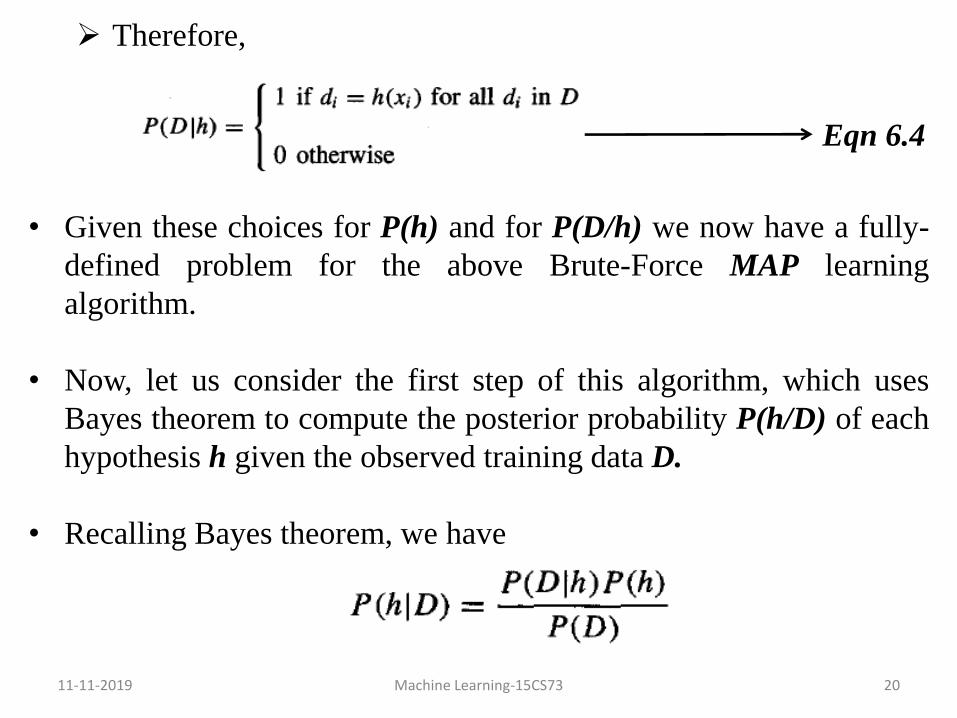
Therefore,

• Given these choices for P(h) and for P(D/h) we now have a fully-

defined problem for the above Brute-Force MAP learning

algorithm.

• Now, let us consider the first step of this algorithm, which uses

Bayes theorem to compute the posterior probability P(h/D) of each

hypothesis h given the observed training data D.

• Recalling Bayes theorem, we have

Eqn 6.4


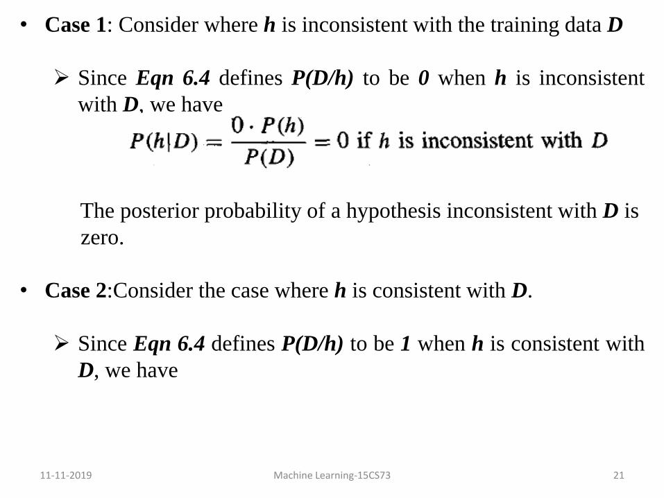
• Case 1: Consider where h is inconsistent with the training data D

Since Eqn 6.4 defines P(D/h) to be 0 when h is inconsistent

with D, we have

The posterior probability of a hypothesis inconsistent with D is

zero.

• Case 2:Consider the case where h is consistent with D.

Since Eqn 6.4 defines P(D/h) to be 1 when h is consistent with

D, we have


where VSH,D is the subset of hypotheses from H that are consistent

with D.


Verification of the value P(D)= |𝑽𝑺𝑯

.𝑫|

|𝑯| for concept learning

• It is easy to verify that P(D)= |𝑽𝑺𝑯

.𝑫|

|𝑯| , because the sum over all

hypotheses of P(h/D) must be one and because the number of

hypotheses from H consistent with D is by definition |VSH,D|

• Alternatively, we can derive P(D) from the theorem of total

probability and the fact that the hypotheses are mutually exclusive

(i.e., (∀i ≠ j)(P(hi ˄ hj) = 0))


• To summarize, Bayes theorem implies that the posterior probability

P(h/D) under our assumed P(h) and P(D/h) is

where |VSH,D| is the number of hypotheses from H consistent with

D.

• The evolution of probabilities associated with hypotheses is

depicted schematically in figure 6.1. Initially figure 6.1(a) shows

all hypotheses have the same probability. As the training data

accumulates (figure 6.1(b) & figure 6.1(c)) the posterior probability

for inconsistent hypotheses becomes zero while the total

probability summing to one is shared equally among the remaining

consistent hypotheses.

Eqn 6.5


Figure 6.1: Evolution of posterior probabilities P(h/D) with increasing training data


MAP Hypotheses and Consistent Learners

• Given the above analysis, every consistent learner outputs a MAP

hypothesis, if we assume a uniform prior probability distribution

over H (i.e., P(hi) = P(hj) for all i, j), and if we assume

deterministic, noise free training data (i.e., P(D/h) = 1 if D and h

are consistent, and 0 otherwise).

• For ex :

Consider the Find-S concept learning algorithm. The Find-S

searches the hypothesis space H from specific to general

hypotheses, outputting a maximally specific consistent

hypothesis.

Because FIND-S outputs a consistent hypothesis, we know that

it will output a MAP hypothesis under the probability

distributions P(h) and P(D/h) defined.


Actually, FIND-S does not explicitly manipulate probabilities

at all-it simply outputs a maximally specific member of the

version space.

However, by identifying distributions for P(h) and P(D/h)

under which its output hypotheses will be MAP hypotheses, we

have a useful way of characterizing the behavior of FIND-S.

• Are there other probability distributions for P(h) and P(D/h)

under which FIND-S outputs MAP hypotheses?

Yes. Because FIND-S outputs a maximally specific hypothesis

from the version space, its output hypothesis will be a MAP

hypothesis relative to any prior probability distribution that

favors more specific hypotheses.


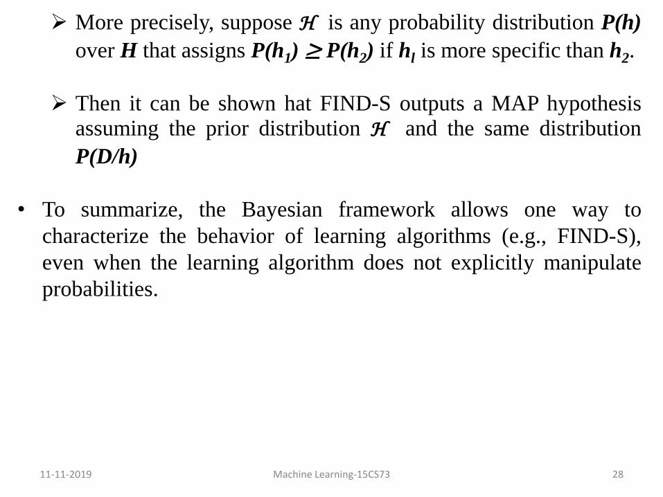
More precisely, suppose H is any probability distribution P(h)

over H that assigns P(h1) ≥ P(h2) if hl is more specific than h2.

Then it can be shown hat FIND-S outputs a MAP hypothesis assuming the prior distribution H and the same distribution

P(D/h)

• To summarize, the Bayesian framework allows one way to

characterize the behavior of learning algorithms (e.g., FIND-S),

even when the learning algorithm does not explicitly manipulate

probabilities.


Definitions of various Probability Terms

Random Variable: A random variable, usually written X, is a

variable whose possible values are numerical outcomes of a random

phenomenon. There are two types of random variables, discrete and continuous.

For ex : Random variable can be defined for a coin flip as follows

X = 𝟏 𝒊𝒇 𝒊𝒕 𝒊𝒔 𝒉𝒆𝒂𝒅𝟎 𝒊𝒇 𝒊𝒕 𝒊𝒔 𝒕𝒂𝒊𝒍

Discrete Random Variable : The variables which can take

distinct/separate values are called discrete random variables.

For ex : Flipping a fair coin, rolling a dice


Continuous Random Variable : The variables which can take any

values in a range are called continuous random variables.

For ex : Height and Weight of the person, Mass of an animal

Probability Distribution : It is a mathematical function that provides

the probabilities of occurrence of different possible outcomes in an

experiment.

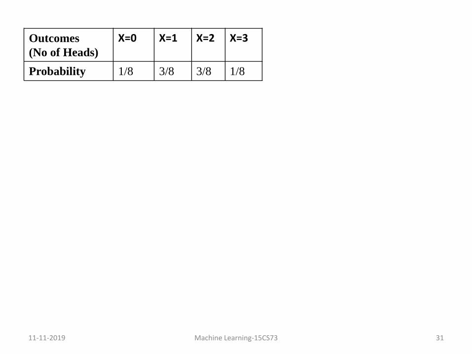
Constructing a probability distribution for random variable

• Let us take random variable,

X = no of heads after 3 flips of a fair coin

• Then the probability distribution table can be written as follows:


Outcomes

(No of Heads)

X=0 X=1 X=2 X=3

Probability 1/8 3/8 3/8 1/8


Maximum Likelihood and Least Squared Error

Hypotheses

• Many learning approaches such as neural network learning, linear

regression and polynomial curve fitting will face a problem of

learning a continuous-valued target function.

• A straightforward Bayesian analysis will show that under certain

assumptions any learning algorithm that minimizes the squared

error between the output hypothesis predictions and the training

data will output a maximum likelihood hypothesis.

• Consider the following problem setting. Learner L considers an

instance space X and a hypothesis space H consisting of some class

of real-valued functions defined over X. (i.e., each h in H is a

function of the form h:X → ℝ, where ℝ represents the set of real

numbers).


• The problem faced by L is to learn an unknown target function f :

X → ℝ drawn from H.

• A set of m training examples is provided, where the target value of

each example is corrupted by random noise drawn according to a

Normal probability distribution.

• More precisely, each training example is a pair of the form <xi, di>

where di = f (xi) + ei. Here f(xi) is the noise-free value of the target

function and ei is a random variable representing the noise.

• It is assumed that the values of the ei are drawn independently and

that they are distributed according to a Normal distribution with

zero mean.

• The task of the learner is to output a maximum likelihood

hypothesis, or, equivalently, a MAP hypothesis assuming all

hypotheses are equally probable a priori.


• As a simple example of such a problem is learning a linear

function, though our analysis applies to learning arbitrary real-

valued functions.

• The figure 6.2 illustrates a linear target function f depicted by the

solid line, and a set of noisy training examples of this target

function.

• The dashed line corresponds to the hypothesis hML with least-

squared training error, hence the maximum likelihood hypothesis.

• The maximum likelihood hypothesis is not necessarily identical to

the correct hypothesis, f, because it is inferred from only a limited

sample of noisy training data.


Figure 6.2 :Learning a real-valued function. The target function f corresponds to the

solid line. The training examples (xi, di) are assumed to have Normally distributed

noise ei with zero mean added to the true target value f(xi). The dashed line

corresponds to the linear function that minimizes the sum of squared errors.


Review of Basic Concepts from Probability Theory

Probability Density Function

• In order to know probabilities over continuous variables such as e,

we must know about probability densities.

• The reason, roughly, is that we wish for the total probability over

all possible values of the random variable to sum to one.

Definition : A probability density function (PDF), or density of a

continuous random variable, is a function that describes the relative

likelihood for this random variable to take on a given value.

• In the case of continuous variables we cannot achieve this by

assigning a finite probability to each of the infinite set of possible

values for the random variable.


• Instead, we take a probability density for continuous variables such

as e and require that the integral of this probability density over all

possible values be one.

• In general we will use lower case p to refer to the probability

density function, to distinguish it from a finite probability P.

• The probability density p(x0) is the limit as 𝜖 goes to zero, of 𝟏

𝝐 times

the probability that x will take on a value in the interval [x0,x0+𝝐)

• The probability density function is


Normal Distribution

• A Normal distribution is a smooth, bell-shaped distribution that can

be completely characterized by its mean and its standard deviation

.

• A Normal distribution (also called a Gaussian distribution) is

defined by the probability density function

A Normal distribution is fully determined by two parameters in the

above formula: and

• If the random variable X follows a normal distribution, then:


The probability that X will fall into the interval (a,b) is given by

𝒑 𝒙 𝒅𝒙𝒃

𝒂

The expected, or mean value of X, E[X], is

E[X] =

The variance of X, Var(X), is

Var(X) = 2

The standard deviation of X, X, is

x =


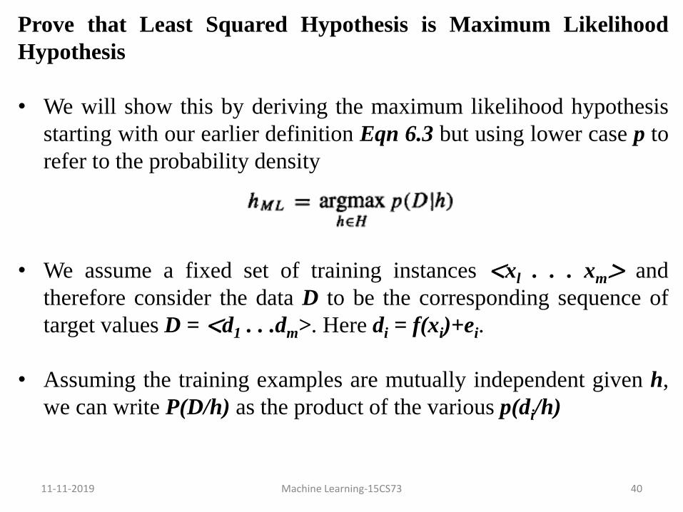
Prove that Least Squared Hypothesis is Maximum Likelihood

Hypothesis

• We will show this by deriving the maximum likelihood hypothesis

starting with our earlier definition Eqn 6.3 but using lower case p to

refer to the probability density

• We assume a fixed set of training instances <xl . . . xm> and

therefore consider the data D to be the corresponding sequence of

target values D = <d1 . . .dm>. Here di = f(xi)+ei.

• Assuming the training examples are mutually independent given h,

we can write P(D/h) as the product of the various p(di/h)


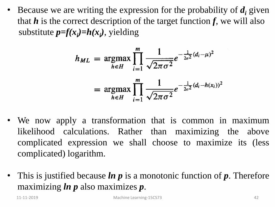
• Given that the noise ei obeys a Normal distribution with zero mean

and unknown variance 2, each di must also obey a Normal

distribution with variance 2 centered around the true target value

f(xi) rather than zero.

• Therefore p(di/h) can be written as a Normal distribution with

variance 2 and mean = f(xi).

• Let us write the formula for this Normal distribution to describe

p(di/h), beginning with the general formula for a Normal

distribution and then substituting appropriate and 2


• Because we are writing the expression for the probability of di given

that h is the correct description of the target function f, we will also

substitute p=f(xi)=h(xi), yielding

• We now apply a transformation that is common in maximum

likelihood calculations. Rather than maximizing the above

complicated expression we shall choose to maximize its (less

complicated) logarithm.

• This is justified because ln p is a monotonic function of p. Therefore

maximizing ln p also maximizes p.


• The first term in this expression is a constant independent of h, and

can therefore be discarded, yielding

• Maximizing this negative quantity is equivalent to minimizing the

corresponding positive quantity.


• Finally, we can again discard constants that are independent of h.

• Thus, Eqn 6.6 shows that the maximum likelihood hypothesis hML

the one that minimizes the sum of the squared errors between the

observed training values di and the hypothesis predictions h(xi)

• This holds under the assumption that the observed training values di

are generated by adding random noise to the true target value, where

this random noise is drawn independently for each example from a

Normal distribution with zero mean.

• As the above derivation makes clear, the squared error term (di-

h(xi))2 directly from the exponent in the definition of the Normal

distribution.

Eqn 6.6


• Notice the structure of the above derivation involves selecting the

hypothesis that maximizes the logarithm of the likelihood (ln

p(D/h)) in order to determine the most probable hypothesis.

• This approach of working with the log likelihood is common to

many Bayesian analyses, because it is often more mathematically

tractable than working directly with the likelihood.

• In all cases, the maximum likelihood hypothesis might not be the

MAP hypothesis, but if one assumes uniform prior probabilities

over the hypotheses then it is.

• Minimizing the sum of squared errors is a common approach in

many neural network, curve fitting, and other approaches to

approximating real-valued functions.


Reason to choose Normal distribution to characterize noise

i. It allows for a mathematically straightforward analysis.

ii. The smooth, bell-shaped distribution is a good approximation to

many types of noise in physical systems.


Maximum Likelihood Hypotheses for Predicting

Probabilities

• Here we will derive criterion for a setting that is common in neural

network learning: learning to predict probabilities.

• Consider the setting in which we wish to learn a nondeterministic

(probabilistic) function f: X→{0,1} , which has two discrete output

values.

• For ex: the instance space X might represent medical patients in

terms of their symptoms, and the target function f(x) might be 1 if

the patient survives the disease and 0 if not.

• In this case we might well expect f to be probabilistic. For ex:

among a collection of patients exhibiting the same set of observable

symptoms, we might find that 92% survive, and 8% do not.


• This unpredictability could arise from our inability to observe all the

important distinguishing features of the patients, or from some

genuinely probabilistic mechanism in the evolution of the disease.

• The effect is that we have a target function f(x) whose output is a

probabilistic function of the input.

• Given this problem setting, we might wish to learn a neural network

(or other real-valued function approximator) whose output is the

probability that f(x)=1.

• In other words, we seek to learn the target function, f': X → [0,1],

such that f'(x) = P(f (x) = 1).

• In order to learn f‘ , we can train a neural network directly from the

observed training examples of f, and derive a maximum likelihood

hypothesis for f‘ .


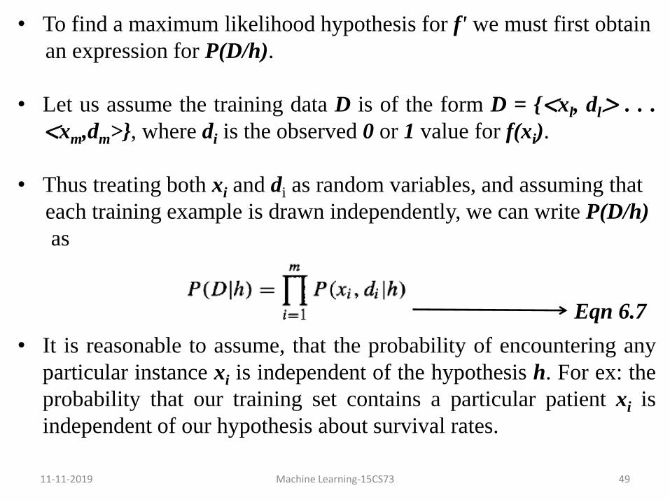
• To find a maximum likelihood hypothesis for f' we must first obtain

an expression for P(D/h).

• Let us assume the training data D is of the form D = {<xl, dl> . . .

<xm,dm>}, where di is the observed 0 or 1 value for f(xi).

• Thus treating both xi and di as random variables, and assuming that

each training example is drawn independently, we can write P(D/h)

as

• It is reasonable to assume, that the probability of encountering any

particular instance xi is independent of the hypothesis h. For ex: the

probability that our training set contains a particular patient xi is

independent of our hypothesis about survival rates.

Eqn 6.7


• When x is independent of h we can rewrite the Eqn 6.7 using the

product rule of probability as

• The probability of P(di/h, xi) of observing di=1 for a single instance

xi , given a world in which hypothesis h holds is h(xi) i.e., P(di=1/h,

xi) = h(xi) and in general

Eqn 6.8

Eqn 6.9


• In order to substitute Eqn 6.9 into Eqn 6.8 , let us re-express Eqn

6.9 in a more mathematically manipulable form, as

• It is easy to verify that the expressions in Eqn 6.9 and Eqn 6.10 are

equivalent. We can use Eqn 6.10 to substitute for P(di/h,xi) in Eqn

6.8 to obtain

Eqn 6.10

Eqn 6.11


• Now we write an expression for the maximum likelihood hypothesis

• The last term is a constant independent of h, so it can be dropped

• As in earlier cases, we will find it easier to work with the log of the

likelihood, yielding

Eqn 6.12

Eqn 6.13


• Eqn 6.13 describes the quantity that must be maximized in order to

obtain the maximum likelihood hypothesis in our current problem

setting.

• This result is analogous to our earlier result showing that

minimizing the sum of squared errors produces the maximum

likelihood hypothesis in the earlier problem setting.


Gradient Search to Maximize Likelihood in a Neural Net

• Let us take G(h,D) to denote the quantity of Maximum Likelihood

hypotheses for the probabilistic target function.

• Our objective here is to derive a weight-training rule for neural

network learning that seeks to maximize G(h,D) using gradient

ascent.

• The gradient of G(h,D) is given by the vector of partial derivatives

of G(h,D) with respect to the various network weights that define

the hypothesis h represented by the learned network.

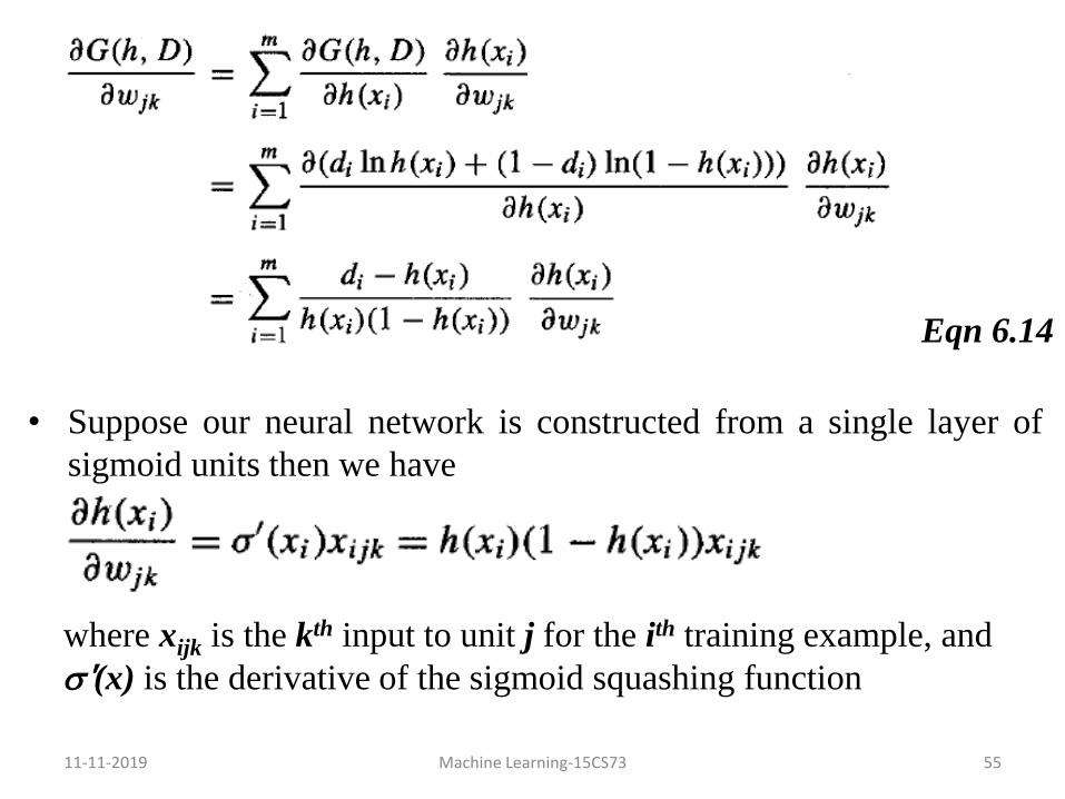
• In this case, the partial derivative of G(h,D) with respect to weight

wjk from input k to unit j is


• Suppose our neural network is constructed from a single layer of

sigmoid units then we have

where xijk is the kth input to unit j for the ith training example, and

'(x) is the derivative of the sigmoid squashing function

Eqn 6.14


• Finally, substituting this expression into Eqn 6.14, we obtain a

simple expression for the derivatives that constitute the gradient

• Because we seek to maximize rather than minimize P(D/h), we

perform gradient ascent rather than gradient descent search. On each

iteration of the search the weight vector is adjusted in the direction

of the gradient, using the weight update rule

where,

Eqn 6.15


where η is a small positive constant that determines the step size of

the gradient ascent search.

• Comparing this weight-update rule to the weight-update rule used

by the Backpropagation algorithm we can get

where,

Notice this is similar to the rule given in Eqn 6.15 except for

the extra term h(x)(l - h(xi)), which is the derivative of the sigmoid

function.


Minimum Description Length Principle

• The Minimum Description Length principle is motivated by

interpreting the definition of hMAP in the light of basic concepts

from information theory.

• Consider the definition of hMAP

which can be equivalently expressed in terms of maximizing the

log2

or alternatively, minimizing the negative of this quantity


• Eqn 6.16 can be interpreted as a statement that short hypotheses are

preferred, assuming a particular representation scheme for encoding

hypotheses and data.

• To explain this, let us take a basic result from information theory:

Consider the problem of designing a code to transmit messages

drawn at random, where the probability of encountering message i is

pi.

• We are interested here in the most compact code i.e., we are

interested in the code that minimizes the expected number of bits we

must transmit in order to encode a message drawn at random.

Eqn 6.16


• Clearly, to minimize the expected code length we should assign

shorter codes to messages that are more probable.

• Shannon and Weaver (1949) showed that the optimal code(i.e., the

code that minimizes the expected message length) assigns –log2pi

bits to encode message i .

• The number of bits required to encode message i using code C will

be referred as the description length of message i with respect to C,

which is denoted as Lc(i).

• Let us interpret Eqn 6.16 in the perspective of the above result from

coding theory

-log2P(h) is the description length of h under the optimal

encoding for the hypothesis space H.


In our notation, 𝑳𝑪𝑯(h) = -log2P(h), where CH is the optimal code

for hypothesis space H.

-log2P(D/h) is the description length of the training data D given

hypothesis h, under its optimal encoding. In our notation,

𝑳𝑪𝑫/𝒉(D/h) = - log2P(D/h), where CD/h is the optimal code for

describing data D assuming that both the sender and receiver

know the hypothesis h.

Therefore we can rewrite Eqn 6.16 to show that hMAP is the

hypothesis h that minimizes the sum given by the description

length of the hypothesis plus the description length of the data

given the hypothesis.


where CH and CD/h are the optimal encodings for H and for D given

h, respectively.

• The Minimum Description Length (MDL) principle recommends

choosing the hypothesis that minimizes the sum of these two

description lengths.

• To apply this principle in practice we must choose specific

encodings or representations appropriate for the given learning task.

• Assuming we use the codes C1 and C2 to represent the hypothesis

and the data given the hypothesis, we can state the MDL principle

as

Eqn 6.17


• The above analysis shows that if we choose C1 to be the optimal

encoding of hypotheses CH, and if we choose C2 to be the optimal

encoding CD/h then hMDL = hMAP.

• Conclusions from MDL Principle

• Does MDL principle prove once and for all that short

hypotheses are best?

• No. We have only shown that if a representation of hypotheses

is chosen so that the size of hypothesis h is -log2P(h), and if a

representation for exceptions is chosen so that the encoding

length of D given h is equal to –log2P(D/h), then the MDL

principle produces MAP hypotheses.



Naïve Bayes Classifier

• One highly practical Bayesian learning method is the naive Bayes

learner, often called the Naive Bayes classifier.

• The Naive Bayes algorithm is a method that uses the probabilities

of each attribute belonging to each class to make a prediction.

• In some domains its performance has been shown to be comparable

to that of neural network and decision tree learning.

• The naive Bayes classifier applies to learning tasks

where each instance x is described by a conjunction

of attribute values and where the target function f(x)

can take on any value from some finite set V.

• A set of training examples of the target function is

provided, and a new instance is presented, described

by the tuple of attribute values <al, a2.. .an>.



• The learner is asked to predict the target value, or classification, for

this new instance.

• The Bayesian approach to classifying the new instance is to assign

the most probable target value, vMAP , given the attribute values < a1

,a2 .. .an > that describe the instance

• We can use Bayes theorem to rewrite this expression as

Eqn 6.19


• Now we could attempt to estimate the two terms in Eqn 6.19 based

on the training data.

• It is easy to estimate each of the P(vj) simply by counting the

frequency with which each target value vj occurs in the training

data.

• However, estimating the different P(al, a2.. . an/vj) terms in this

fashion is not feasible unless we have a very, very large set of

training data.

• The problem is that the number of these terms is equal to the

number of possible instances times the number of possible target

values.

• Therefore, we need to see every instance in the instance space many

times in order to obtain reliable estimates.


Assumption

The naive Bayes classifier is based on the simplifying assumption that

the attribute values are conditionally independent given the target

value.

• From this assumption it is possible to say that given the target value

of the instance, the probability of observing the conjunction

a1,a2…an is just the product of probabilities for the individual

attributes:

P(a1,a2….an/vj) = 𝑷(𝒂𝒊/𝒗𝒋𝒊 )

Substituting this into Eqn 6.19, we have the approach used by the

Naive Bayes classifier.


where vNB denotes the target value output by the Naïve Bayes

classifier.

• Thus, in a in a Naive Bayes classifier the number of distinct P(ai/vj)

terms that must estimated from the training data is just the number

of distinct attribute values times the number of distinct target

values- a much smaller number compared to estimating

P(a1,a2,….an/vj).

• To summarize, the naive Bayes learning method involves a learning

step in which the various P(vj) and P(ai/vj) terms are estimated,

based on their frequencies over the training data.

Eqn 6.20


• The set of these estimates corresponds to the learned hypothesis.

This hypothesis is then used to classify each new instance by

applying the rule in Eqn 6.20.

• Whenever the naive Bayes assumption of conditional independence

is satisfied, this naive Bayes classification vNB is identical to the

MAP classification.

• One interesting difference between the naive Bayes learning method

and other learning methods we have considered is that there is no

explicit search through the space of possible hypotheses.


An Illustrative Example

• Let us apply the naive Bayes classifier to a concept learning

problem we considered during our discussion of decision tree

learning: classifying days according to whether someone will play

tennis(PlayTennis).

• Table 3.2 provides a set of 14 training examples of the target

concept PlayTennis, where each day is described by the attributes

Outlook, Temperature, Humidity, and Wind.

• Here we use the naive Bayes classifier and the training data from

this Table 3.2 to classify the following novel instance:

<Outlook = sunny, Temperature = cool, Humidity = high, Wind =

strong>

Table 3.2:Training examples for the target concept PlayTennis

Day Outlook Temperature Humidity Wind PlayTennis

D1 Sunny Hot High Weak No

D2 Sunny Hot High Strong No

D3 Overcast Hot High Weak Yes

D4 Rain Mild High Weak Yes

D5 Rain Cool Normal Weak Yes

D6 Rain Cool Normal Strong No

D7 Overcast Cool Normal Strong Yes

D8 Sunny Mild High Weak No

D9 Sunny Cool Normal Weak Yes

D10 Rain Mild Normal Weak Yes

D11 Sunny Mild Normal Strong Yes

D12 Overcast Mild High Strong Yes

D13 Overcast Hot Normal Weak Yes

D14 Rain Mild High Strong No



• Our task is to predict the target value (yes or no) of the target

concept PlayTennis for this new instance.

• Instantiating Eqn 6.20 to fit the current task, the target value VNB is

given by


Estimating probabilities of attribute values and target value from

training data

Probabilities of Target Value(PlayTennis)

Probabilities of Outlook Attribute values

PlayTennis P(Yes)/P(No)

Yes 9 9/14

No 5 5/14

Total 14

Yes No P(Yes) P(No)

Sunny 2 3 2/9 3/5

Overcast 4 0 4/9 0/5

Rain 3 2 3/9 2/5

Total 9 5


Probabilities of Temperature Attribute Values

Probabilities of Humidity Attribute Values

Yes No P(Yes) P(No)

Hot 2 2 2/9 4/5

Mild 4 2 4/9 2/5

Cool 3 1 3/9 1/5

Total 9 5

Yes No P(Yes) P(No)

Normal 6 1 6/9 1/5

High 3 4 3/9 4/5

Total 9 5


Probabilities of Wind Attribute Values

• Using these probability estimates and similar estimates for the

remaining attribute values, we calculate vNB according to Eqn 6.21

as follows:

For vj = Yes

VNB = P(Yes) P(Sunny/Yes) P(Cool/Yes) P(High/Yes) P(Strong/Yes)

= 9/14 * 2/9 * 3/9 * 3/9 * 3/9

= 0.00529

Yes No P(Yes) P(No)

Strong 3 3 3/9 3/5

Weak 6 2 6/9 2/5

Total 9 5


For vj = No

VNB = P(No) P(Sunny/No) P(Cool/No) P(High/No) P(Strong/No)

= 5/14 * 3/5 * 1/5 * 4/5 * 3/5

= 0.020571

• Thus, the naive Bayes classifier assigns the target value PlayTennis

= No to this new instance, based on the probability estimates

learned from the training data.

Table 3.2:Training examples for the target concept Buys_Computer

RID Age Income Student Credit_Rating Buys_Computer

1 Youth High No Fair No

2 Youth High No Excellent No

3 Middle_aged High No Fair Yes

4 Senior Medium No Fair Yes

5 Senior Low Yes Fair Yes

6 Senior Low Yes Excellent No

7 Middle_aged Low Yes Excellent Yes

8 Youth Medium No Fair No

9 Youth Low Yes Fair Yes

10 Senior Medium Yes Fair Yes

11 Youth Medium Yes Excellent Yes

12 Middle_aged Medium No Excellent Yes

13 Middle_aged High Yes Fair Yes

14 Senior Medium No Excellent No



Estimating Probabilities

• Till now, we have estimated probabilities by the fraction of times the

event is observed to occur over the total number of opportunities.

• For ex : we estimated P(Wind = strong|Play Tennis = no) by the

fraction 𝑛

𝑐

𝑛 where n = 5 is the total number of training examples for

which PlayTennis = no, and n= 3 is the number of these for which

Wind = strong.

• While this observed fraction provides a good estimate of the

probability in many cases, it provides poor estimates when nc is very

small.

• To see the difficulty, for time being let us imagine that the value of

P(Wind = strong | PlayTennis = no) is .08 and that we have a

sample containing only 5 examples for which PlayTennis = no.


• Then the most probable value for nc is 0 which raises two

difficulties:

i.𝑛

𝑐

𝑛 produces a biased underestimate of the probability.

ii. when this probability estimate is zero, this probability term

will dominate the Bayes classifier if the future query contains

Wind = strong.

• To avoid this difficulty we can adopt a Bayesian approach to

estimating the probability, using the m-estimate defined as follows:

Eqn 6.22


• Here, nc and n are defined as before, p is our prior estimate of the

probability we wish to determine and m is a constant called the

equivalent sample size which determines how heavily to weight p

relative to the observed data.

• A typical method for choosing p in the absence of other information

is to assume uniform priors, i.e., if an attribute has k possible values

we set p = 𝟏

𝒌 .

• For ex: in estimating P(Wind = Strong | PlayTennis = no) we note

the attribute Wind has two possible values, so uniform priors would

correspond to choosing p = 0.5.

• Note that in Eqn 6.22 if m is zero, then m-estimate is equivalent to

the simple fraction 𝒏

𝒄

𝒏 .


• If both n and m are nonzero, then the observed fraction 𝒏

𝒄

𝒏 and prior

p will be combined according to the weight m.

• The reason m is called the equivalent sample size is that Eqn 6.22

can be interpreted as augmenting the n actual observations by an

additional m virtual samples distributed according to p.


Bayesian Belief Networks

• The naive Bayes classifier makes significant use of the assumption

that the values of the attributes a1 . . .an are conditionally

independent given the target value v.

• This assumption dramatically reduces the complexity of learning the

target function.

• When it is met, the naive Bayes classifier outputs the optimal Bayes

classification. However, in many cases this conditional

independence assumption is clearly overly restrictive.

• A Bayesian belief network describes the probability distribution

governing a set of variables by specifying a set of conditional

independence assumptions along with a set of conditional

probabilities.


• In contrast to the naive Bayes classifier, which assumes that all the

variables are conditionally independent given the value of the target

variable, Bayesian belief networks allow stating conditional

independence assumptions that apply to subsets of the variables.

• Thus, Bayesian belief networks provide an intermediate approach

that is less constraining than the global assumption of conditional

independence made by the naive Bayes classifier.

• Bayesian belief networks more tractable than avoiding conditional

independence assumptions altogether.

• In general, a Bayesian belief network describes the probability

distribution over a set of variables. Consider an arbitrary set of

random variables Y1 . . . Yn, where each variable Yi can take on the

set of possible values V(Yi).


• We define the joint space of the set of variables Y to be the cross

product V(Yl) x V(Y2) x . . . V(Yn). Each item in the joint space

corresponds to one of the possible assignments of values to the tuple

of variables <Yl . . . Yn>.

• The probability distribution over this joint space is called the joint

probability distribution.

• A Bayesian belief network describes the joint probability

distribution for a set of variables.


Conditional Independence

• Let X, Y, and Z be three discrete-valued random variables. We say

that X is conditionally independent of Y given Z if the probability

distribution governing X is independent of the value of Y given a

value for Z i.e., if

where xiϵV(X), yj ϵ V(Y), and zkϵ V(Z).

• We commonly write the above expression in abbreviated form as

P(X | Y, Z) = P(X | Z). This definition of conditional independence

can be extended to sets of variables as well.

• We say that the set of variables X1 . . . Xl is conditionally

independent of the set of variables Yl . . . Ym given the set of

variables Z1 . . . Zn if


• The correspondence can be drawn between this definition and our

use of conditional ,independence in the definition of the naive Bayes

classifier.


Bayesian Belief Network Representation

• A Bayesian belief network (Bayesian network for short) represents

the joint probability distribution for a set of variables.

• For example, the Bayesian network in figure 6.3.1 represents the

joint probability distribution over the boolean variables Storm,

Lightning, Thunder, ForestFire, Campfire, and BusTourGroup.

• In general, a Bayesian network represents the joint probability

distribution by specifying a set of conditional independence

assumptions (represented by a directed acyclic graph), together with

sets of local conditional probabilities.

• Each variable in the joint space is represented by a node in the

Bayesian network


Bayesian Belief Network Representation

• A Bayesian belief network (Bayesian network for short) represents

the joint probability distribution for a set of variables.

• For example, the Bayesian network in figure 6.3.1 represents the

joint probability distribution over the boolean variables Storm,

Lightning, Thunder, ForestFire, Campfire, and BusTourGroup.

• In general, a Bayesian network represents the joint probability

distribution by specifying a set of conditional independence

assumptions (represented by a directed acyclic graph), together with

sets of local conditional probabilities.

• Each variable in the joint space is represented by a node in the

Bayesian network


Figure 6.3.1: Bayesian Belief Network


• For each variable two types of information are specified.

i. The network arcs represent the assertion that the variable is

conditionally independent of its nondescendants in the network

given its immediate predecessors in the network. We say X is a

descendant of Y if there is a directed path from Y to X.

ii. A conditional probability table is given for each variable,

describing the probability distribution for that variable given

the values of its immediate predecessors.

• The joint probability for any desired assignment of values <y1 , . . . ,

yn> to the tuple of network variables <Y1 . . . Yn> can be computed

by the formula


where Parents(Yi) denotes the set of immediate predecessors of Yi

in the network.

• Let us illustrate the Bayesian network given in figure 6.3.1 which

represents the joint probability distribution of boolean variables

Storm, Lightning, Thunder, ForestFire, Campfire, and

BusTourGroup.

• Consider the node Campfire. The network nodes and arcs represent

the assertion that Campfire is conditionally independent of its

nondescendants Lightning and Thunder, given its immediate

parents Storm and BusTourGroup.

• This means that once we know the value of the variables Storm and

BusTourGroup, the variables Lightning and Thunder provide no

additional information about Campfire.


• The figure 6.3.2 below shows the conditional probability table

associated with the variable Campfire.

• The top left entry in this table, for ex: expresses the assertion that

P(Campfire=True| Storm=True, BusTourGroup=True)=0.4

• Note this table provides only the conditional probabilities of

Campfire given its parent variables Storm and BusTourGroup.

Figure 6.3.2: The conditional Probability Table for Campfire node


• The set of local conditional probability tables for all the variables,

together with the set of conditional independence assumptions

described by the network, describe the full joint probability

distribution for the network.

• One attractive feature of Bayesian belief networks is that they allow

a convenient way to represent causal knowledge such as the fact that

Lightning causes Thunder.


Learning in Bayesian Belief Networks

• Can we devise effective algorithms for learning Bayesian belief

networks from training data?

• Several different settings for this learning problem can be

considered.

i. First, the network structure might be given in advance, or it

might have to be inferred from the training data.

ii. Second, all the network variables might be directly observable

in each training example, or some might be unobservable.

• In the case where the network structure is given in advance and the

variables are fully observable in the training examples, learning the

conditional probability tables is straightforward.


• We simply estimate the conditional probability table entries just as

we would for a naive Bayes classifier.

• In the case where the network structure is given but only some of

the variable values are observable in the training data, the learning

problem is more difficult.

• This problem is somewhat analogous to learning the weights for the

hidden units in an artificial neural network, where the input and

output node values are given but the hidden unit values are left

unspecified by the training examples.

• Russell et al.(1995) proposed a gradient ascent procedure that learns

entries in conditional probability tables.

• This gradient ascent procedure searches through a space of

hypotheses that corresponds to the set of all possible entries for the

conditional probability tables.


Learning Structure of Bayesian Networks

• Learning Bayesian networks when the network structure is not

known in advance is also difficult.

• Cooper and Herskovits (1992) present a Bayesian scoring metric for

choosing among alternative networks.

• They also present a heuristic search algorithm called K2 for learning

network structure when the data is fully observable.

• Constraint-based approaches to learning Bayesian network structure

have also been developed


The EM Algorithm

• In many practical learning settings, only a subset of the relevant

instance features might be observable.

• For ex : in training our or using the Bayesian belief network we

might have data where only a subset of the network variables

Storm, Lightning, Thunder, ForestFire, Campfire, and

BusTourGroup have been observed.

• Many approaches have been proposed to handle the problem of

learning in the presence of unobserved variables.

• The EM algorithm (Dempster et al. 1977), a widely used approach

for learning in the presence of unobserved variables.


• The EM algorithm can be used even for variables whose value is

never directly observed, provided the general form of the

probability distribution governing these variables is known.

• The EM algorithm has been used to train Bayesian belief networks

as well as radial basis function networks.

• The EM algorithm is also the basis for many unsupervised

clustering algorithms.


Estimating Means of k Gaussians

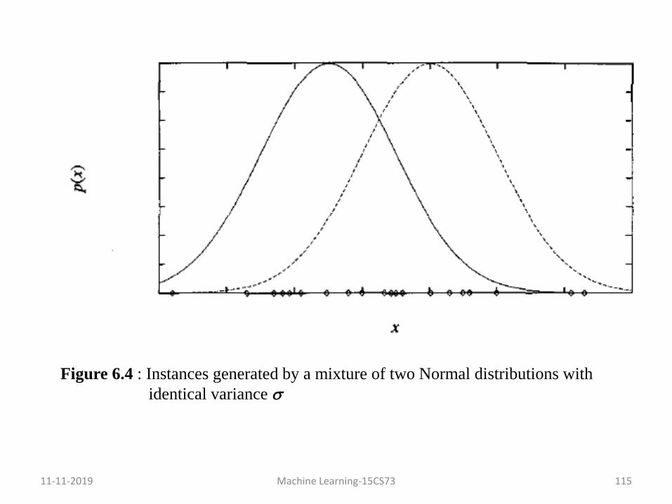
• Consider a problem in which the data D is a set of instances

generated by a probability distribution that is a mixture of k distinct

Normal distributions.

• This problem setting is illustrated in figure 6.4 for the case where k

= 2 and where the instances are the points shown along the x-axis.

• Each instance is generated using a two-step process.

i. One of the k Normal distributions is selected at random.

ii. A single random instance xi is generated according to this

selected distribution.

This process is repeated to generate a set of data points as shown in

figure 6.4


Figure 6.4 : Instances generated by a mixture of two Normal distributions with

identical variance


• Let us consider a special case, where the selection of the single

Normal distribution at each step is based on choosing each with

uniform probability, where each of the k Normal distributions has

the same variance 2.

• The learning task is to output a hypothesis h = <1… k> that

describes the means of each of the k distributions.

• This task involves finding a maximum likelihood hypothesis for

these means; i.e., a hypothesis h that maximizes p(D/h).

• It is easy to calculate the maximum likelihood hypothesis for the

mean of a single Normal distribution given the observed data

instances x1, x2, . . . , xm drawn from this single distribution


• Restating Eqn 6.6 using our current notation, we have

• In this case, the sum of squared errors is minimized by the sample

mean

Eqn 6.27

Eqn 6.28


Necessity for EM Algorithm

• Our problem involves a mixture of k different Normal distributions,

and we cannot observe which instances were generated by which

distribution.

• Thus, we have a prototypical example of a problem involving

hidden variables.

• In the example of figure 6.4 we can think of the full description of

each instance as the triple <xi , zi1 , zi2>, where xi is the observed

value of the ith instance and where zi1 and zi2 indicate which of the two

Normal distributions was used to generate the value xi.

• Here xi is the observed variable in the description of the instance,

and zi1 and zi2 are hidden variables.


• If the values of zi1 and zi2 were observed, we could use Eqn 6.27 to

solve for the means 1 and 2. Because they are not, we will instead

use the EM algorithm.

• Applied to our k-means problem the EM algorithm searches for a

maximum likelihood hypothesis by repeatedly re-estimating the

expected values of the hidden variables zij given its current

hypothesis <1.....k> then recalculating the maximum likelihood

hypothesis using these expected values for the hidden variables.

Describing an instance of EM

algorithm

• Applied to the problem of estimating the two means

for figure 6.4, the EM algorithm first initializes the

hypothesis to h=<1,2>, where 1 and 2 are

arbitrary initial values.

• It then iteratively re-estimates h by repeating the

following two steps until the procedure converges to

a stationary value for h.



Step 1: Calculate the expected value E[zij] of each hidden variable zij,

assuming the current hypothesis h= <1,2> holds.

Step 2: Calculate a new maximum likelihood hypothesis h' = <1', 2'>, assuming the value taken on by each hidden variable zij

is its expected value E[zij] calculated in Step 1. Then replace

the hypothesis h= <1,2> by the new hypothesis h' = <1', 2'> and iterate.

Implementation of steps in practice

• Step 1 must calculate the expected value of each zij .

This E[zij] is just the probability that instance xi was

generated by the jth Normal distribution



• Thus the first step is implemented by substituting the current values

<1, 2> and the observed xi into the above expression.

• In the second step we use the E[zij] calculated during Step 1 to

derive a new maximum likelihood hypothesis h' = <1', 2'>. The

maximum likelihood hypothesis in this case is given by


• Our new expression is just the weighted sample mean for j, with

each instance weighted by the expectation E[zij] that it was

generated by the jth Normal distribution.


General Statement of EM Algorithm

• The EM algorithm can be applied in many settings where we wish

to estimate some set of parameters θ that describe an underlying

probability distribution, given only the observed portion of the full

data produced by this distribution.

• In the two-means example the parameters of interest were θ =

<1,2>, and the full data were the triples <xi, zi1, zi2 > of which

only the xi were observed.

• In general let X = {xl, . . . , xm} denote the observed data in a set of

m independently drawn instances, let Z = {z1, . . . , zm} denote the

unobserved data in these same instances, and let Y = X U Z denote

the full data.


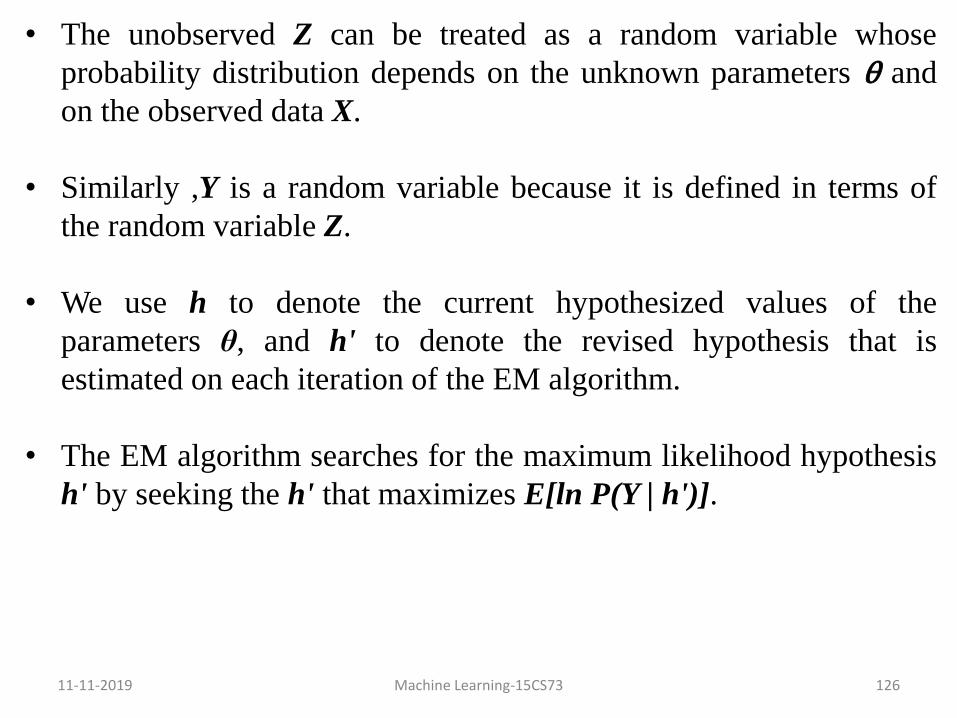
• The unobserved Z can be treated as a random variable whose

probability distribution depends on the unknown parameters θ and

on the observed data X.

• Similarly ,Y is a random variable because it is defined in terms of

the random variable Z.

• We use h to denote the current hypothesized values of the

parameters θ, and h' to denote the revised hypothesis that is

estimated on each iteration of the EM algorithm.

• The EM algorithm searches for the maximum likelihood hypothesis

h' by seeking the h' that maximizes E[ln P(Y | h')].


• Let us consider exactly what this expression signifies

i. First, P(Y | h') is the likelihood of the full data Y given

hypothesis h'. It is reasonable that we wish to find a h' that

maximizes some function of this quantity.

ii. Second, maximizing the logarithm of this quantity ln P(Y | h') also maximizes P(Y | h').

iii. Third, we introduce the expected value E[ln P(Y | h')] because

the full data Y is itself a random variable.

• Given that the full data Y is a combination of the observed data X

and unobserved data Z, we must average over the possible values of

the unobserved Z, weighting each according to its probability.

• In other words we take the expected value E[ln P(Y | h')] over the

probability distribution governing the random variable Y.


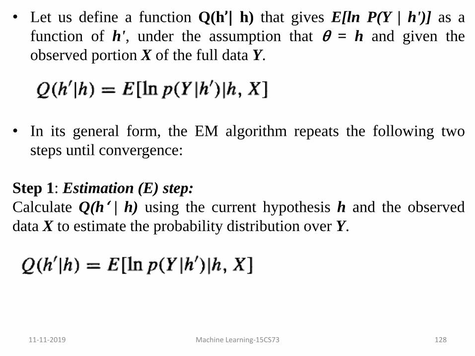
• Let us define a function Q(h’| h) that gives E[ln P(Y | h')] as a

function of h', under the assumption that θ = h and given the

observed portion X of the full data Y.

• In its general form, the EM algorithm repeats the following two

steps until convergence:

Step 1: Estimation (E) step:

Calculate Q(h‘ | h) using the current hypothesis h and the observed

data X to estimate the probability distribution over Y.


Step 2: Maximization(M) step:

Replace hypothesis h by the hypothesis h' that maximizes this Q

function.

When the function Q is continuous, the EM algorithm converges to a

stationary point of the likelihood function P(Y/h').


Derivation of k Means Algorithm

• To illustrate the general EM algorithm, let us use it to derive the

algorithm for estimating the means of a mixture of k Normal

distributions.

• In the k-means objective is to estimate the parameters θ = <1..k>

that define the means of the k Normal distributions.

• We are given the observed data X = {<xi>}.The hidden variables Z

= {<zi1,. . . , zik>} in this case indicate which of the k Normal

distributions was used to generate xi.

• To apply EM we must derive an expression for Q(h‘ | h) that applies

to our k-means problem.

• First, let us derive an expression for ln p(Y | h')


• The probability p(yi | h') of a single instance yi = <xi , zi1 , . . . zik> if

the full data can be written as

• Given this probability for a single instance p(yi \ h'), the logarithm

of the probability ln P(Y \ h') for all m instances in the data is


• Finally we must take the expected value of this ln P(Y \ h') over the

probability distribution governing Y. The above expression for ln

P(Y \ h') is a linear function of these zij. In general, for any function

f(z) that is a linear function of z, the following equality holds

E[f(z)] = f(E[z])

• This general fact about linear functions allows us to write


• To summarize, the function Q(h‘ | h) for the k means problem is

where h' = <1', . . . ,k'> and where E[zij] is calculated based on

the current hypothesis h and observed data X. We know that

Thus, the first (estimation) step of the EM algorithm defines the Q

function based on the estimated E[zij] terms.

• The second (maximization) step then finds the values 1' . . . k' that

maximize this Q function. In the current case

Eqn 6.29


Thus, the maximum likelihood hypothesis here minimizes a weighted

sum of squared errors, where the contribution of each instance xi to the

error that defines j' is weighted by E[zij]

• The quantity given by Eqn 6.30 is minimized by setting each j' to

the weighted sample mean

Eqn 6.30

Eqn 6.31

Documents

Module 4: Chapter 6 Bayesian Learning