Module 4: Buckling of 2D Simply Supported Beam

UCONN ANSYS –Module 3 Page 1

Module 4: Buckling of 2D Simply Supported Beam

Table of Contents Page Number

Problem Description 2

Theory 2

Geometry 4

Preprocessor 7

Element Type 7

Real Constants and Material Properties 8

Meshing 9

Solution 11

Static Solution 11

Eigenvalue 14

Mode Shape 15

General Postprocessor 16

Results 18

Validation 18


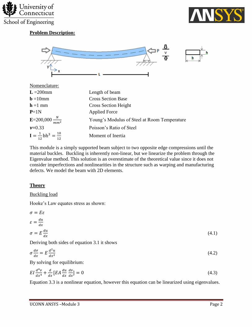
Problem Description:

Nomenclature:

L =200mm Length of beam

b =10mm Cross Section Base

h =1 mm Cross Section Height

P=1N Applied Force

E=200,000

Young’s Modulus of Steel at Room Temperature

=0.33 Poisson’s Ratio of Steel

Moment of Inertia

This module is a simply supported beam subject to two opposite edge compressions until the

material buckles. Buckling is inherently non-linear, but we linearize the problem through the

Eigenvalue method. This solution is an overestimate of the theoretical value since it does not

consider imperfections and nonlinearities in the structure such as warping and manufacturing

defects. We model the beam with 2D elements.

Theory

Buckling load

Hooke’s Law equates stress as shown:

(4.1)

Deriving both sides of equation 3.1 it shows

(4.2)

By solving for equilibrium:

(4.3)

Equation 3.3 is a nonlinear equation, however this equation can be linearized using eigenvalues.

y x


Since:

(4.4)

Then:

(4.5)

Plugging in Equation 3.1 for stress we find:

(4.6)

Plugging Equation 3.6 into Equation 3.3, Equation 3.6 becomes

(4.7)

Which is simplifies to:

(4.8)

By integrating two times Equation 3.8 becomes

(4.9)

At the fixed end (x=0), v=0,

, thus 0

At the supported end (x=L), v=0,

, thus 0

Equation 3.9 becomes

(4.10)

Equation 3.6 represents the Differential Equation for a Sin Wave

√

√

(4.11)

A and B are arbitrary constants which are calculated based on Boundary Conditions.

At the fixed end (x=0), v=0 proving B=0. Equation 3.11 becomes

√

(4.12)

But A cannot equal zero or this problem is trivial.

At the supported end (x=L), v=0 Equation 12 becomes

√

(4.13)

Since A cannot equal zero, ( ) must equal zero:

Sin(nπ)=0 for n=(0, 1, 2, 3, 4…..)


So:

√

n ≠ 0 or it is trivial (4.14)

We are interested in finding P which is the Critical Buckling Load. Since n can be any integer

greater than zero and a continuous beam has theoretically infinite degrees of freedom there are

infinite amount of eigenvalues ( ).

(4.15)

Where the lowest Buckling Load is at

(4.16)

This is an over estimate so there are certain correction factors (C) to account for this. (C) is

dependent on the beam constraints.

(4.17)

Where C=1 for a fixed-simply supported beam.

So the Critical Buckling Load is

= 41.124 N (4.18)

Geometry

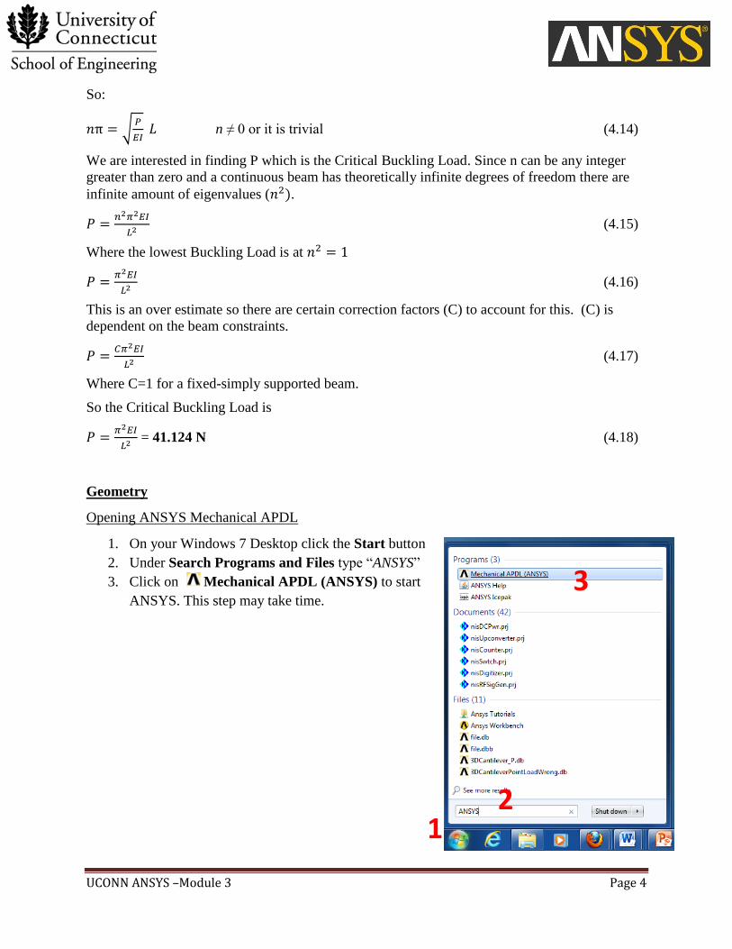
Opening ANSYS Mechanical APDL

1. On your Windows 7 Desktop click the Start button

2. Under Search Programs and Files type “ANSYS”

3. Click on Mechanical APDL (ANSYS) to start

ANSYS. This step may take time.

3

1

2


Preferences

1. Go to Main Menu -> Preferences

2. Check the box that says Structural

3. Click OK

Title:

To add a title

1. Utility Menu -> ANSYS Toolbar -> type /prep7 -> enter

2. Utility Menu -> ANSYS Toolbar -> type /Title, “ Title Name” -> enter

1

2

3

2


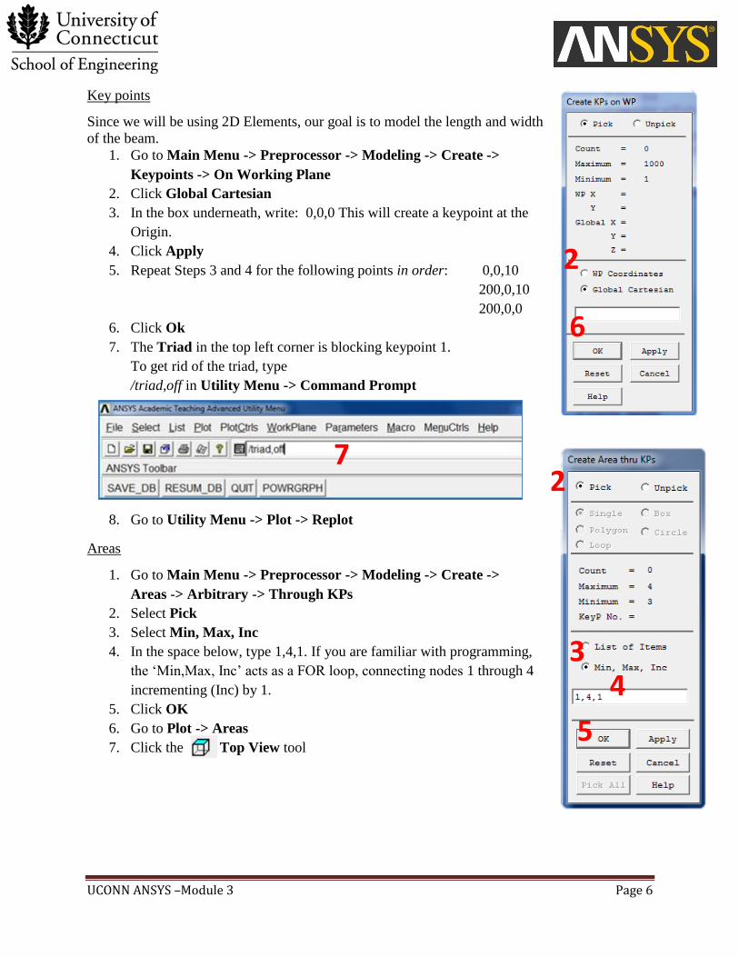
Key points

Since we will be using 2D Elements, our goal is to model the length and width

of the beam.

1. Go to Main Menu -> Preprocessor -> Modeling -> Create ->

Keypoints -> On Working Plane

2. Click Global Cartesian

3. In the box underneath, write: 0,0,0 This will create a keypoint at the

Origin.

4. Click Apply

5. Repeat Steps 3 and 4 for the following points in order: 0,0,10

200,0,10

200,0,0

6. Click Ok

7. The Triad in the top left corner is blocking keypoint 1.

To get rid of the triad, type

/triad,off in Utility Menu -> Command Prompt

8. Go to Utility Menu -> Plot -> Replot

Areas

1. Go to Main Menu -> Preprocessor -> Modeling -> Create ->

Areas -> Arbitrary -> Through KPs

2. Select Pick

3. Select Min, Max, Inc

4. In the space below, type 1,4,1. If you are familiar with programming,

the ‘Min,Max, Inc’ acts as a FOR loop, connecting nodes 1 through 4

incrementing (Inc) by 1.

5. Click OK

6. Go to Plot -> Areas

7. Click the Top View tool

6

7

2

3

4

5

2


Your beam should look as below:

Saving Geometry

We will be using the geometry we have just created for 3 modules. Thus it would be convenient

to save the geometry so that it does not have to be made again from scratch.

1. Go to File -> Save As …

2. Under Save Database to

pick a name for the Geometry.

For this tutorial, we will name

the file ‘Buckling simply

supported’

3. Under Directories: pick the

Folder you would like to save the

.db file to.

4. Click OK

Preprocessor

Element Type

1. Go to Main Menu -> Preprocessor -> Element Type -> Add/Edit/Delete

2. Click Add

3. Click Shell -> 4node181

4. Click OK

4

2

3

3

4


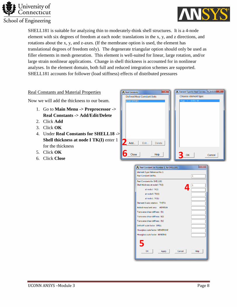
SHELL181 is suitable for analyzing thin to moderately-think shell structures. It is a 4-node

element with six degrees of freedom at each node: translations in the x, y, and z directions, and

rotations about the x, y, and z-axes. (If the membrane option is used, the element has

translational degrees of freedom only). The degenerate triangular option should only be used as

filler elements in mesh generation. This element is well-suited for linear, large rotation, and/or

large strain nonlinear applications. Change in shell thickness is accounted for in nonlinear

analyses. In the element domain, both full and reduced integration schemes are supported.

SHELL181 accounts for follower (load stiffness) effects of distributed pressures

Real Constants and Material Properties

Now we will add the thickness to our beam.

1. Go to Main Menu -> Preprocessor ->

Real Constants -> Add/Edit/Delete

2. Click Add

3. Click OK

4. Under Real Constants for SHELL18 ->

Shell thickness at node I TK(I) enter 1

for the thickness

5. Click OK

6. Click Close

2

3

4

5

6


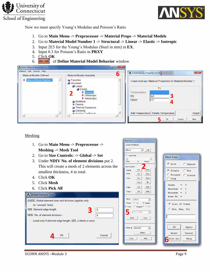
Now we must specify Young’s Modulus and Poisson’s Ratio

1. Go to Main Menu -> Preprocessor -> Material Props -> Material Models

2. Go to Material Model Number 1 -> Structural -> Linear -> Elastic -> Isotropic

3. Input 2E5 for the Young’s Modulus (Steel in mm) in EX.

4. Input 0.3 for Poisson’s Ratio in PRXY

5. Click OK

6. of Define Material Model Behavior window

Meshing

1. Go to Main Menu -> Preprocessor ->

Meshing -> Mesh Tool

2. Go to Size Controls: -> Global -> Set

3. Under NDIV No. of element divisions put 2.

This will create a mesh of 2 elements across the

smallest thickness, 4 in total.

4. Click OK

5. Click Mesh

6. Click Pick All

3 4

5

2

6

2

3

4

5

6


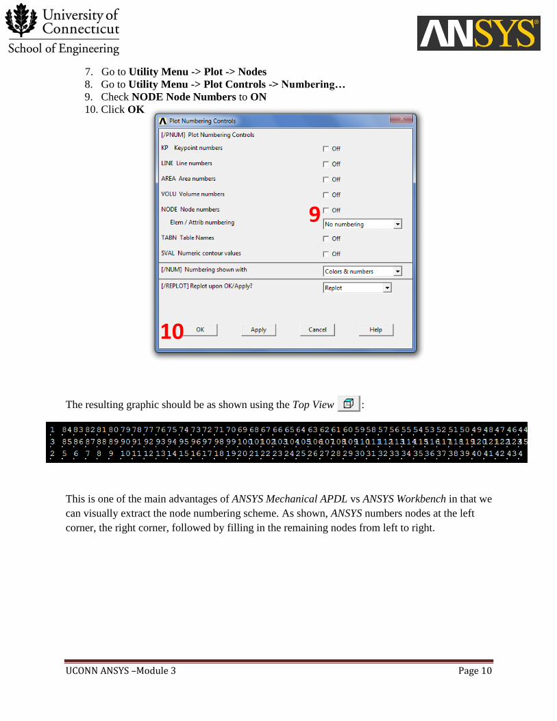
7. Go to Utility Menu -> Plot -> Nodes

8. Go to Utility Menu -> Plot Controls -> Numbering…

9. Check NODE Node Numbers to ON

10. Click OK

The resulting graphic should be as shown using the Top View :

This is one of the main advantages of ANSYS Mechanical APDL vs ANSYS Workbench in that we

can visually extract the node numbering scheme. As shown, ANSYS numbers nodes at the left

corner, the right corner, followed by filling in the remaining nodes from left to right.

9

10


Solution

There are two types of solution menus that ANSYS APDL provides; the Abridged solution menu

and the Unabridged solution menu. Before specifying the loads on the beam, it is crucial to be in

the correct menu.

Go to Main Menu -> Solution -> Unabridged menu

This is shown as the last tab in the Solution menu. If this reads “Abridged menu” you are

already in the Unabridged solution menu.

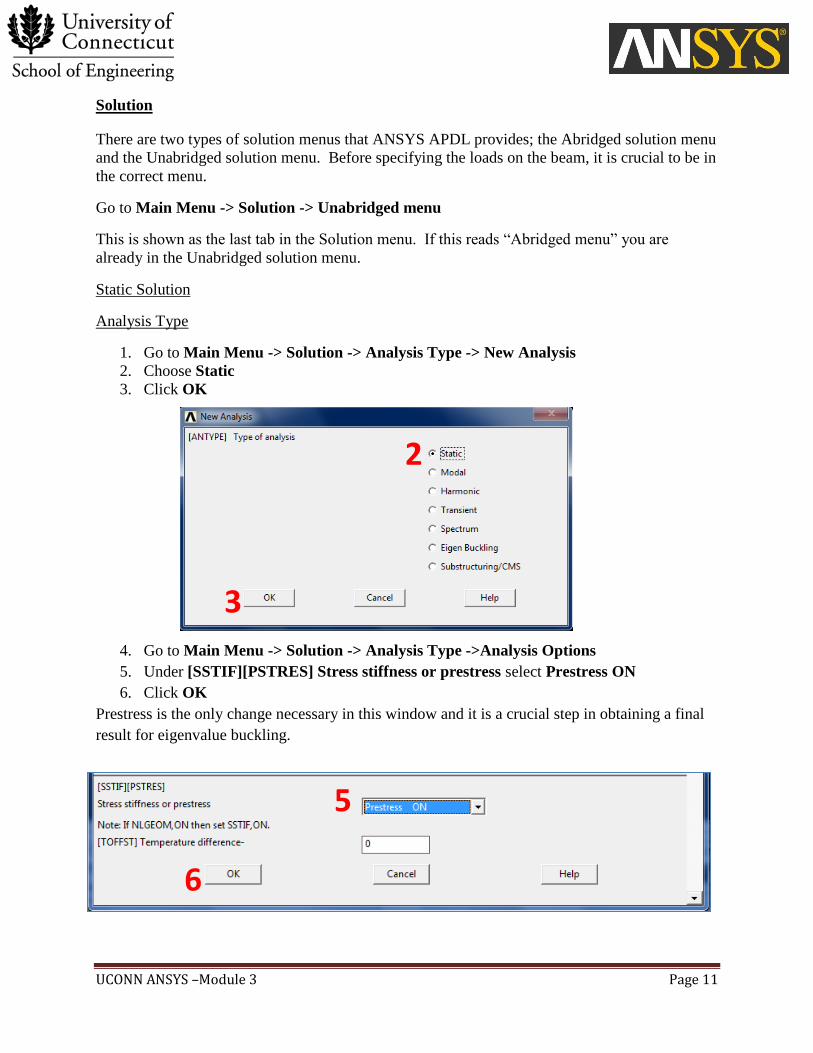
Static Solution

Analysis Type

1. Go to Main Menu -> Solution -> Analysis Type -> New Analysis

2. Choose Static

3. Click OK

4. Go to Main Menu -> Solution -> Analysis Type ->Analysis Options

5. Under [SSTIF][PSTRES] Stress stiffness or prestress select Prestress ON

6. Click OK

Prestress is the only change necessary in this window and it is a crucial step in obtaining a final

result for eigenvalue buckling.

2

3

5

6


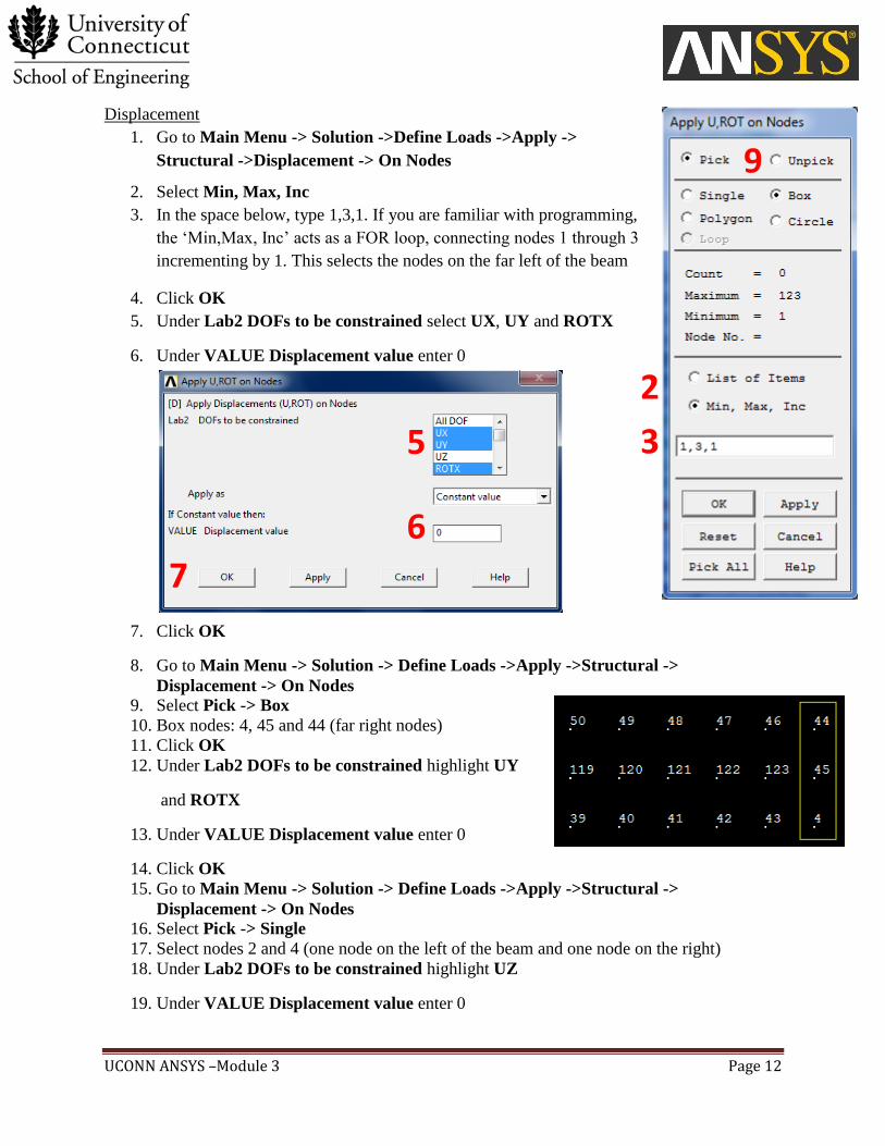
Displacement

1. Go to Main Menu -> Solution ->Define Loads ->Apply ->

Structural ->Displacement -> On Nodes

2. Select Min, Max, Inc

3. In the space below, type 1,3,1. If you are familiar with programming,

the ‘Min,Max, Inc’ acts as a FOR loop, connecting nodes 1 through 3

incrementing by 1. This selects the nodes on the far left of the beam

4. Click OK

5. Under Lab2 DOFs to be constrained select UX, UY and ROTX

6. Under VALUE Displacement value enter 0

7. Click OK

8. Go to Main Menu -> Solution -> Define Loads ->Apply ->Structural ->

Displacement -> On Nodes 9. Select Pick -> Box

10. Box nodes: 4, 45 and 44 (far right nodes)

11. Click OK

12. Under Lab2 DOFs to be constrained highlight UY

and ROTX


14. Click OK

15. Go to Main Menu -> Solution -> Define Loads ->Apply ->Structural ->

Displacement -> On Nodes 16. Select Pick -> Single

17. Select nodes 2 and 4 (one node on the left of the beam and one node on the right)

18. Under Lab2 DOFs to be constrained highlight UZ


2

5

6

7

3

9


20. Click OK

This creates the fixed end on the left and roller support on the right, while constraining

movement in the Z-direction

Loads

1. Go to Main Menu -> Solution -> Define Loads ->

Apply -> Structural ->Force/Moment -> On Nodes

2. Select Pick -> Single -> List of Items

3. In the space provided, type 45. Press OK.

4. Under Direction of force/mom select FX

5. Under VALUE Force/moment value enter -1

6. Click OK

WARNING: UX, UY and ROTX might already be highlighted, if so, leave

UY and ROTX highlighted and click UX to remove it from the selection.

Failure to only constrain UY and ROTX will result in incorrect results.

2

3

4

5

6

USEFUL TIP: The force value is only a magnitude of 1 because

eigenvalues are calculated by a factor of the load applied, so having a

force of 1 will make the eigenvalue answer equal to the critical load.


Solve

1. Go to Main Menu -> Solution -> Solve -> Current LS

2. Go to Main Menu -> Finish

Eigenvalue

1. Go to Main Menu -> Solution -> Analysis Type -> New Analysis

2. Choose Eigen Buckling

3. Click OKGo to Main Menu -> Solution -> Analysis Type ->Analysis Options

4. Under NMODE No. of modes to extract input 4

5. Click OK



2

3

5

6

6


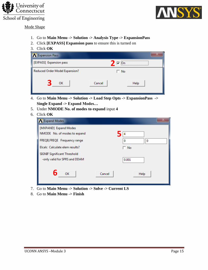
Mode Shape

1. Go to Main Menu -> Solution -> Analysis Type -> ExpansionPass

2. Click [EXPASS] Expansion pass to ensure this is turned on

3. Click OK

4. Go to Main Menu -> Solution -> Load Step Opts -> ExpansionPass ->

Single Expand -> Expand Modes…

5. Under NMODE No. of modes to expand input 4

6. Click OK



2

3

5

6


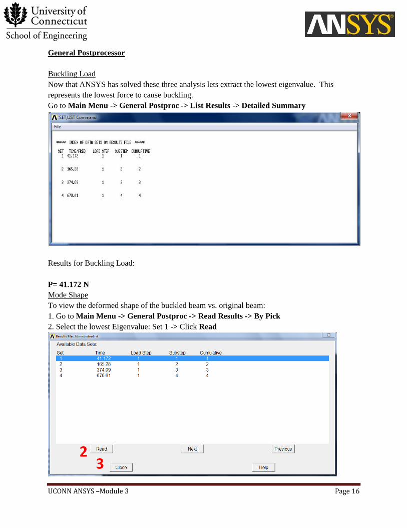
General Postprocessor

Buckling Load

Now that ANSYS has solved these three analysis lets extract the lowest eigenvalue. This

represents the lowest force to cause buckling.

Go to Main Menu -> General Postproc -> List Results -> Detailed Summary

Results for Buckling Load:

P= 41.172 N

Mode Shape

To view the deformed shape of the buckled beam vs. original beam:

1. Go to Main Menu -> General Postproc -> Read Results -> By Pick

2. Select the lowest Eigenvalue: Set 1 -> Click Read

3

2


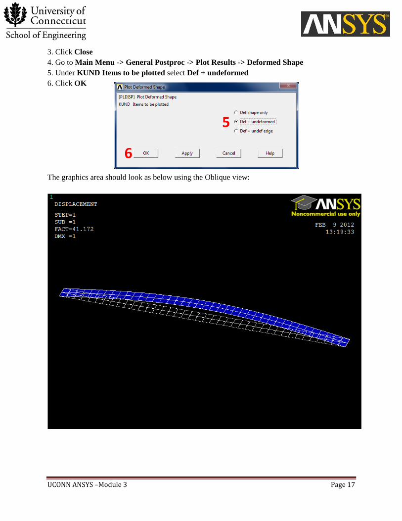
3. Click Close

4. Go to Main Menu -> General Postproc -> Plot Results -> Deformed Shape

5. Under KUND Items to be plotted select Def + undeformed

6. Click OK

The graphics area should look as below using the Oblique view:

6

5


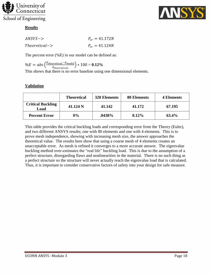
Results

The percent error (%E) in our model can be defined as:

(

) = 0.12%

This shows that there is no error baseline using one dimensional elements.

Validation

Theoretical 320 Elements 80 Elements 4 Elements

Critical Buckling

Load 41.124 N 41.142 41.172 67.195

Percent Error 0% .0438% 0.12% 63.4%

This table provides the critical buckling loads and corresponding error from the Theory (Euler),

and two different ANSYS results; one with 80 elements and one with 4 elements. This is to

prove mesh independence, showing with increasing mesh size, the answer approaches the

theoretical value. The results here show that using a coarse mesh of 4 elements creates an

unacceptable error. As mesh is refined it converges to a more accurate answer. The eigenvalue

buckling method over-estimates the “real life” buckling load. This is due to the assumption of a

perfect structure, disregarding flaws and nonlinearities in the material. There is no such thing as

a perfect structure so the structure will never actually reach the eigenvalue load that is calculated.

Thus, it is important to consider conservative factors of safety into your design for safe measure.

Documents

Module 4: Buckling of 2D Simply Supported Beam