Atmospheric Boundary Layers:

An introduction and model intercomparisons

Bert Holtslag

Lecture for Summer school on “Land-Atmosphere Interactions“,

Valsavarenche, Valle d'Aosta (Italy), 22 June, 2015

Meteorology and Air Quality Department

2

The lower layer of the Atmosphere influenced by the presence of the earth’s surface due to:

Friction, Surface Heating (Convection) or Cooling

Important characteristics are Turbulence and Diurnal Cycle!

Atmospheric Boundary layer (ABL)

Daytime ABL: 500-2000 m Nighttime ABL: 10-500 m

(Stull, 1988)

3

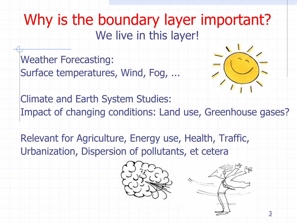
Why is the boundary layer important? We live in this layer!

Weather Forecasting:

Surface temperatures, Wind, Fog, ...

Climate and Earth System Studies:

Impact of changing conditions: Land use, Greenhouse gases?

Relevant for Agriculture, Energy use, Health, Traffic,

Urbanization, Dispersion of pollutants, et cetera

The interaction of the land-surface with the atmospheric boundary

layer includes many processes and complex feedback mechanisms

(Figure by Mike Ek, see also Ek and Holtslag, 2004)

ECMWF/GABLS workshop 7-10 November 2011 (5)

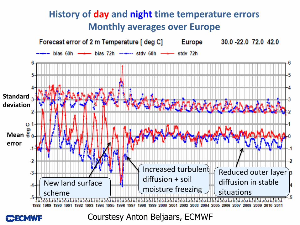
History of day and night time temperature errors Monthly averages over Europe

Increased turbulent diffusion + soil moisture freezing

Standard deviation

Mean error

New land surface scheme

Reduced outer layer diffusion in stable situations

Courstesy Anton Beljaars, ECMWF

Daytime Clear Convective Boundary Layer over Land

6

285 290 2950

500

1000

1500

temperature [K]

he

igh

t [m

]conv ectiv e

boundary layer

thermal inv ersion

free atmosphere

Why does an inversion form at ABL top?

Convection over land

Intermezzo Potential temperature

7

Temperature that a parcel will have if it is moved (dry) adiabatically to a reference level (P0=1000 hPa or z=0)

pd CR

P

PT

/

0

29

00

m

For dry adiabatic process the potential temperature is constant! Actual temperature decrease (increase) for rising (sinking) parcel due to air expansion (compression)

Poisson’s equation

8

www.knmi.nl/~bosveld

Intense daytime turbulent mixing gives same potential temperature, but nighttime surface cooling leads to strong vertical gradients!

Example: Cabauw tower observations 4 November 2006 (diurnal cycle of potential temperatures at 2 to 200 m)

9

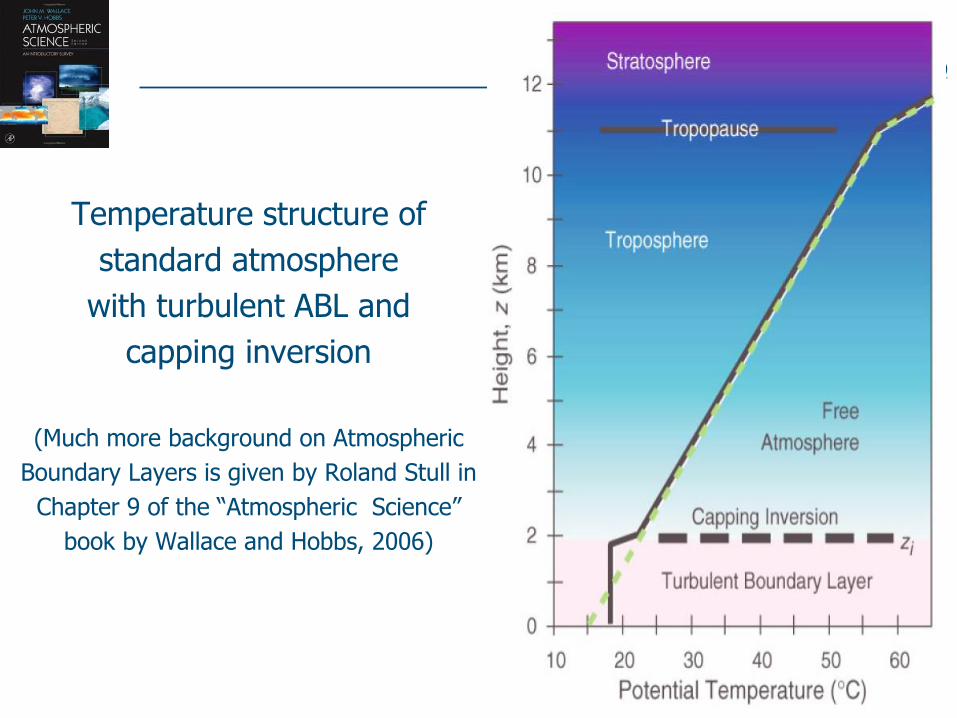
Temperature structure of

standard atmosphere

with turbulent ABL and

capping inversion

(Much more background on Atmospheric

Boundary Layers is given by Roland Stull in

Chapter 9 of the “Atmospheric Science”

book by Wallace and Hobbs, 2006)

10

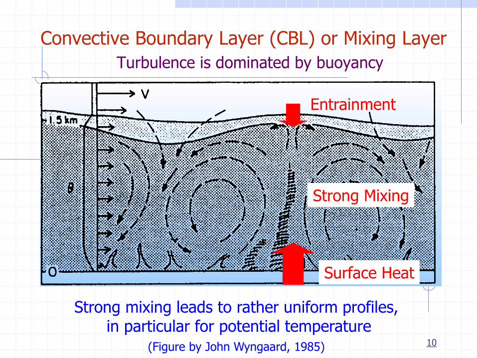
Convective Boundary Layer (CBL) or Mixing Layer

Turbulence is dominated by buoyancy

Strong mixing leads to rather uniform profiles, in particular for potential temperature

(Figure by John Wyngaard, 1985)

Entrainment

Surface Heat

Strong Mixing

11

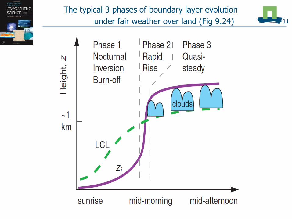
The typical 3 phases of boundary layer evolution

under fair weather over land (Fig 9.24)

Cumulus clouds

How does the land surface impact on the onset of Cumulus?

Role of soil moisture and atmospheric processes?

Courtesy Michael Ek (NCEP)

wet soil dry soil

stronger inversion

weaker inversion

dry soil

How to quantify?

θ

Δθ

γθ

q

Δq

γq

(Ek and Mahrt, 1994; Ek&Holtslag 2004)

Consider Relative Humidity (RH) tendency at boundary layer top

Use mixed-layer bulk model for the tendency terms

Analytical result

ne: non-evaporative processes, including entrainment and boundary layer growth

Confirmed with Cabauw (wet soils) and AMMA observations (dry soils)

(Westra et al, 2012, JHM)

Evaporative fraction

(Ek & Holtslag 2004, JHM)

Boundary layer over heterogeneous terrain 15

16

Stable boundary layer

Turbulence by friction, surface cooling stabilizes Large gradients in temperature and wind

(Figure by John Wyngaard, 1985)

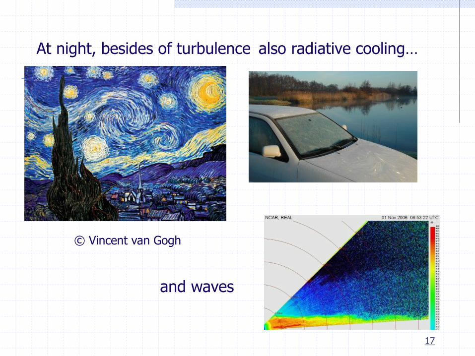
17

At night, besides of turbulence

and waves

also radiative cooling…

© Vincent van Gogh

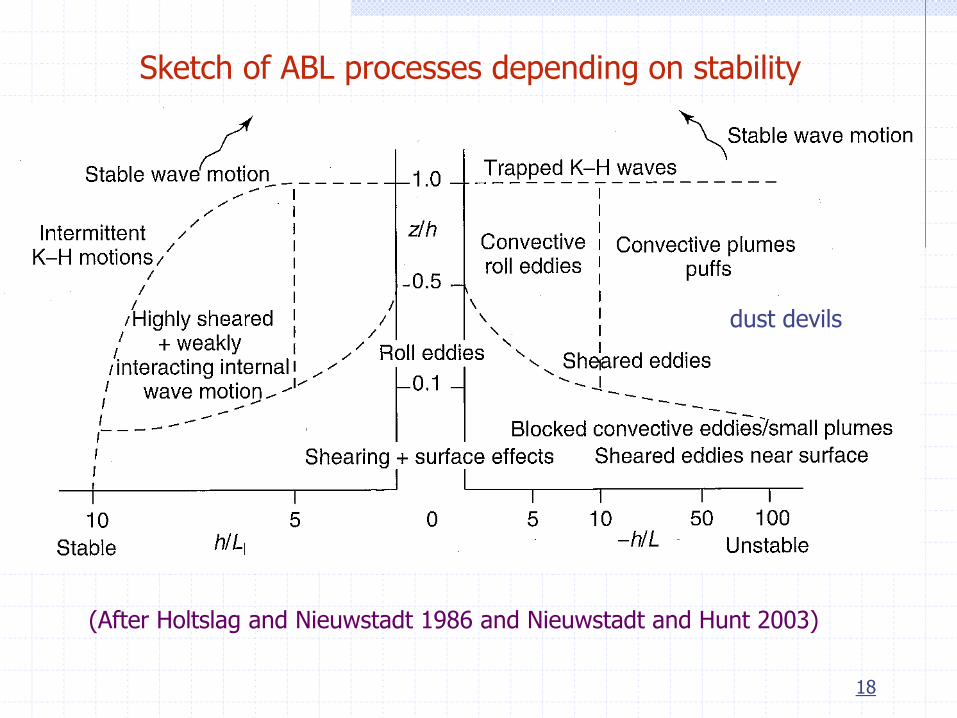
18

(After Holtslag and Nieuwstadt 1986 and Nieuwstadt and Hunt 2003)

Sketch of ABL processes depending on stability

dust devils

19

Stable (nocturnal) Boundary Layer

Residual Layer

Noon Sunset Midnight Sunrise Noon

Free Atmosphere

Convective

Mixed Layer

Diurnal cycle over land

unstable stable

20

Stable (nocturnal) Boundary Layer

Residual Layer

Noon Sunset Midnight Sunrise Noon

Free Atmosphere

Convective

Mixed Layer

Mean profiles

unstable

U

Ugeo

stable

U

Ugeo

Low Level Jet

21

Turbulence in boundary layer

U

1) Wind shear (S) 2) Buoyancy (B)

+ +

- Day: S>0 B>0

Night: S>0 B<0

Day N

ight

22

Observations of temperature fluctuations at several

heights over flat terrain

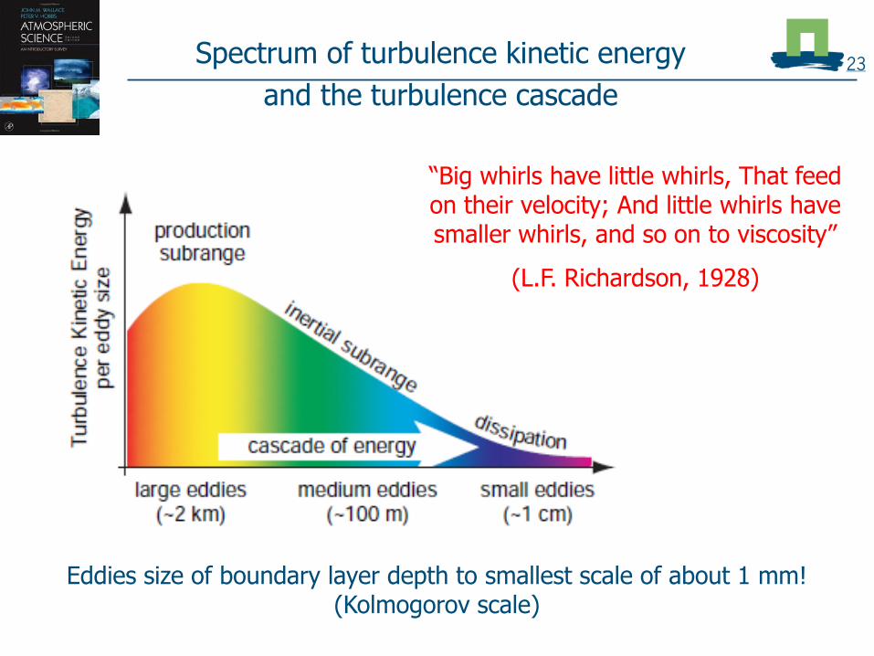
23 Spectrum of turbulence kinetic energy

and the turbulence cascade

Eddies size of boundary layer depth to smallest scale of about 1 mm! (Kolmogorov scale)

“Big whirls have little whirls, That feed on their velocity; And little whirls have smaller whirls, and so on to viscosity”

(L.F. Richardson, 1928)

24 Turbulent heat flux and high frequency data

0',0'

0',0'

'

'

ww

and

w

thus

www

'

Reynolds decomposition

''

''''

''

ww

wwww

www

Flux is a co-variance

w'w

w

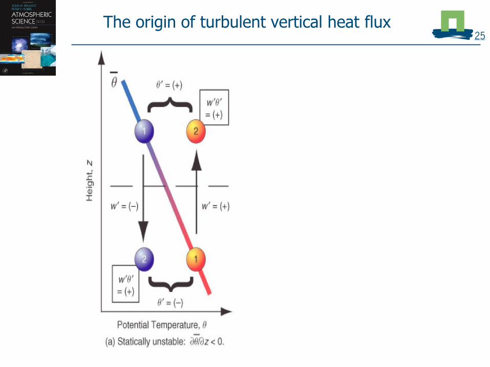
25 The origin of turbulent vertical heat flux

26 The origin of turbulent vertical heat flux

27 Turbulent heat flux

232

''

''

0

''''

sm

JK

s

m

Kkg

J

m

kg

m

W

wCH

ww

w

wwwww

p

near surface, thus:

Turbulent heat flux

Break

28

Meteosat observations versus ECMWF predictions (T1279 ~ 15 km) (Courtesy MeteoSat and ECMWF)

Progress in the Atmospheric Sciences: Connecting scales

Atmospheric Budget Equations

Sub-grid processes

Discretization

Budget equation for potential temperature after Reynolds decomposition

31

....''

...''

zKw

z

w

zW

yV

xU

tdt

d

Similar equations for wind and any ‘conserved’ quantity C

(specific humidity, tracers,…)

Can be solved for given initial and surface conditions, and if the diffusivities (K) are known

K: Eddy diffusivity for heat

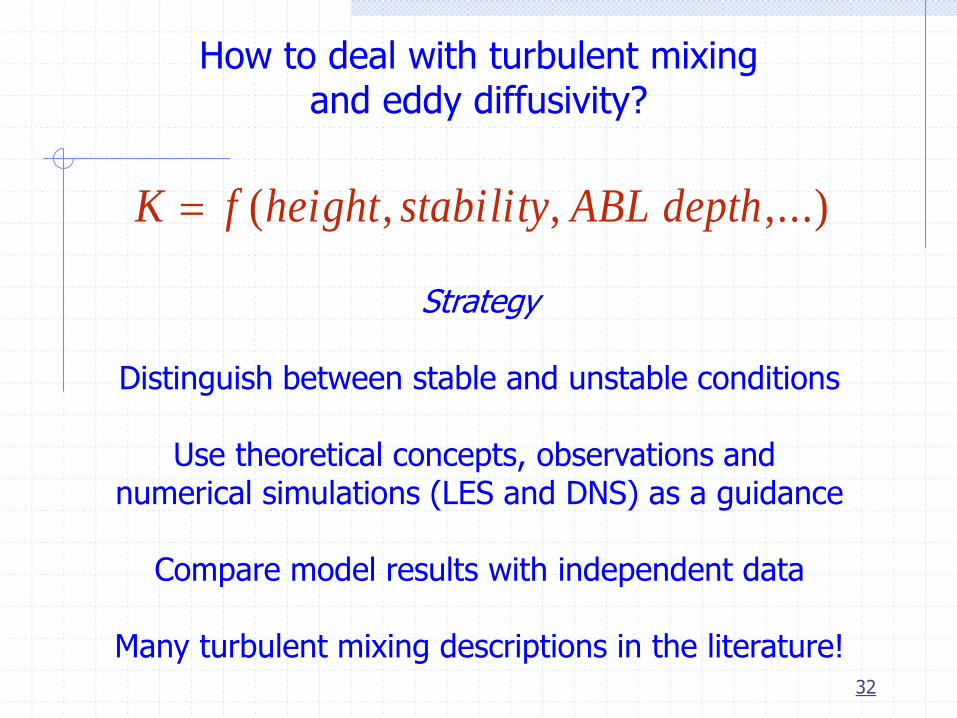
32

How to deal with turbulent mixing and eddy diffusivity?

,...),,( depthABLstabilityheightfK

Strategy

Distinguish between stable and unstable conditions

Use theoretical concepts, observations and numerical simulations (LES and DNS) as a guidance

Compare model results with independent data

Many turbulent mixing descriptions in the literature!

Non-local mixing in convective boundary layers

Use profile function for eddy-diffusivity and non-local (‘counter-gradient’) corrections

zKw

Deardorff (1966, 1972) Troen and Mahrt (1986)

Holtslag and Boville (1993) Large et al (1994)

Hong and Pan (1996) Beljaars and Viterbo (1998)

Lock et al (2000) et cetera

This approach is now widely adopted (e.g., NCAR, NCEP, UKMO, ECMWF,...), but details differ...

34

Flux-Gradient Theory (first order closure)

2

,

2

:

)(

''

z

U

z

gRi

scalelengthl

RiFlz

UK

z

CKcw

hm

Turbulent Flux

Diffusivity K depends on characteristics of turbulent flow

Richardson number (measure for local stability)

35

Stable boundary layer mixing

Three alternatives for stability functions of heat and momentum

LTG: Louis et al (1982)

MO: Extended Monin-Obukhov type, in agreement with Cabauw tower observations (Beljaars and Holtslag, 1991)

Fm

Fh

LTG

Revised LTG MO

Revised LTG

LTG MO

Enhanced friction needed in models

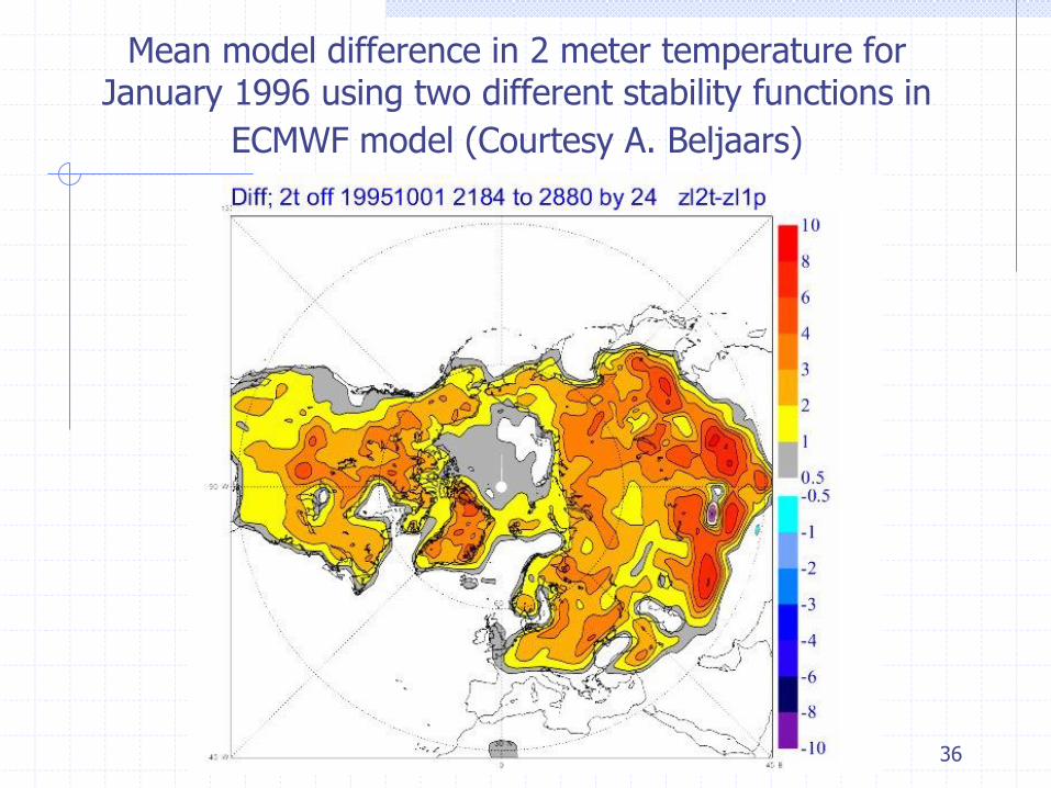
36

Mean model difference in 2 meter temperature for January 1996 using two different stability functions in

ECMWF model (Courtesy A. Beljaars)

37

Turbulent Kinetic Energy (TKE) closure scheme (applied in many atmospheric models…)

TKElK

nDissipatioTransportBuoyShearAdvt

TKE

TKE represents the major characteristics of turbulence

How to do the length scale?

Is local gradient assumption valid?

Many proposals have been made for various boundary layers

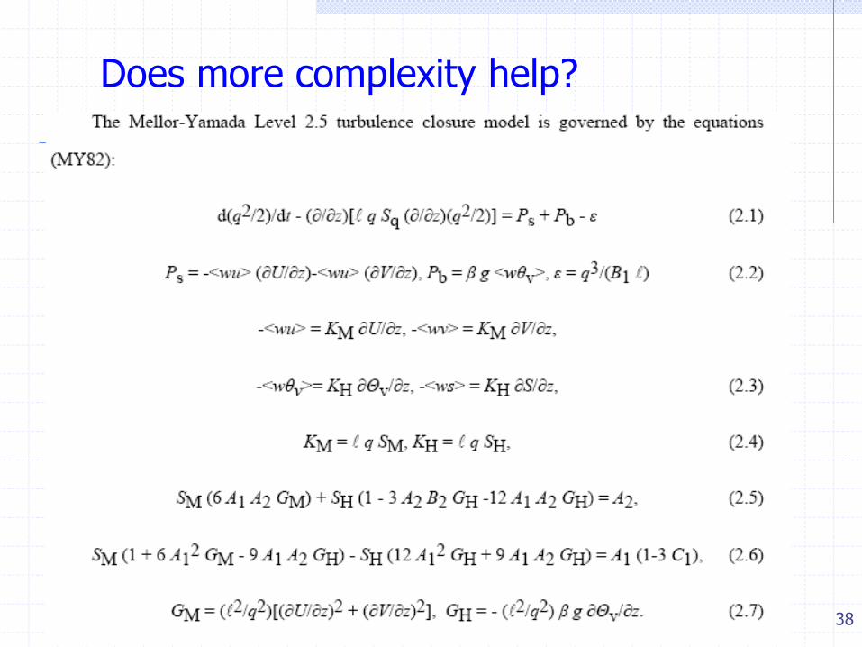
Does more complexity help?

38

Modeling Atmospheric Boundary Layers: It is still a challenge!

Atmospheric models do have problems in representing

the stable boundary layer and the diurnal cycle

Sensitivity to details in mixing formulation Strategy

Enhance understanding by benchmark studies

over land and ice in comparison with observations and fine scale numerical model results

So far focus on clear skies!

GABLS1 GABLS2 GABLS3

LES as reference Data (CASES99) Data (CABAUW)

Academic set up Idealized forcings Realistic forcings

Prescribed Ts Prescribed Ts

Full coupling (SCM)

Prescribed Ts (LES)

No Radiation No Radiation Radiation included

Turbulent mixing Diurnal cycle Low levet jet +

transitions

GEWEX Atmospheric Boundary Layer Studies (GABLS) provides platform for model intercomparison and development to

benefit studies of Climate, Weather, Air Quality and Wind Energy

LES: Large Eddy Simulation; SCM: Single Column Model

41

GABLS3: SCM and LES model studies

GABLS3-LES

00 Z 02 Jul

09 Z 02 Jul

12 Z 01 July 2006

12 Z 02 Jul

Initialization Profiles Cabauw tower, Profiler, De Bilt Sounding Geostrophic Wind (time-height dependent) Similar for both SCM and LES

Large-scale Advection (time-height dependent) Similar for both SCM and LES Surface Boundary Conditions Cabauw tower

GABLS3-SCM

Cabauw tower (KNMI, NL)

GABLS3 intercomparison of

Single Column versions (SCM) of operational and research models

(Coordinated by Fred Bosveld, KNMI)

Note: Each SCM uses its

own radiation and land surface scheme

interacting with the boundary layer scheme

on usual resolution! (Nlev is number of

vertical levels in whole atmosphere)

Name Institute Nlev BL.Scheme Skin

ALADIN Meteo France 41 TKE No

AROME Meteo France 41 TKE No

GLBL38 Met Office 38 K (long tail) Yes

UK4L70 Met Office 70 K (short tail) Yes

D91 WUR 91 K Yes

GEM Env. Cananda 89 TKE-l No

ACM2 NOAA 155 K+non-local No

WRF YSU NOAA 61 K No

WRF MYJ NOAA 61 TKE-l No

WRFTEMF NOAA 61 Total E No

COSMO DWD 41

GFS NCEP 57 K Yes

WRF MYJ NCEP 57 TKE-l Yes

WRF YSU NCEP 57 K Yes

MIUU MISU 65 2nd order

MUSC KNMI 41 TKE-l No

RACMO KNMI 80 TKE Yes

C31R1 ECMWF 80 K Yes

CLUBB UWM 250 Higher order No

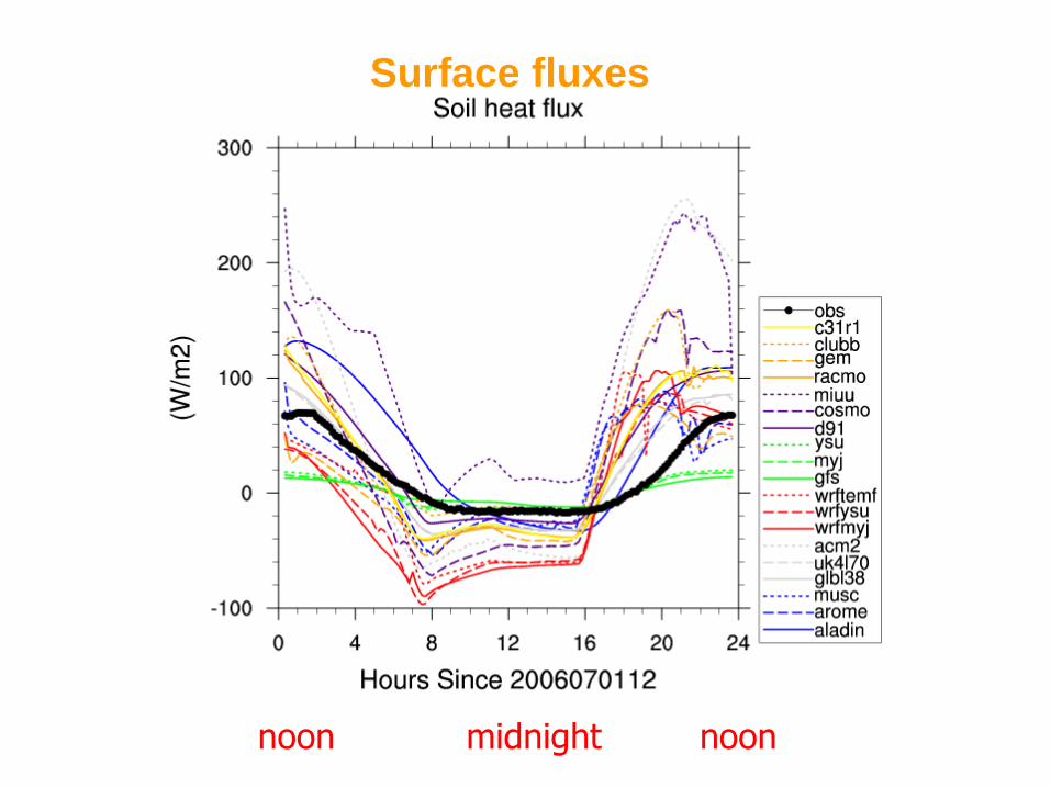
Surface fluxes

noon midnight noon

Surface fluxes

noon midnight noon

Surface fluxes

noon midnight noon

Surface fluxes

noon midnight noon

noon midnight noon

Surface parameters

noon midnight noon

Low level jet

noon midnight noon

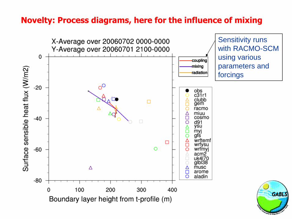
Novelty: Process diagrams, here for the influence of mixing

Sensitivity runs

with RACMO-SCM

using various

parameters and

forcings

ISARS-2010, Paris, 28-30 June 2010

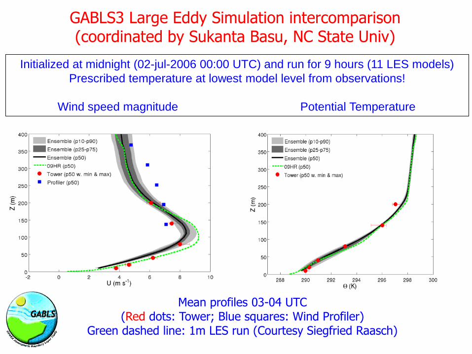
GABLS3 Large Eddy Simulation intercomparison (coordinated by Sukanta Basu, NC State Univ)

Initialized at midnight (02-jul-2006 00:00 UTC) and run for 9 hours (11 LES models)

Prescribed temperature at lowest model level from observations!

Wind speed magnitude Potential Temperature

Mean profiles 03-04 UTC (Red dots: Tower; Blue squares: Wind Profiler)

Green dashed line: 1m LES run (Courtesy Siegfried Raasch)

ISARS-2010, Paris, 28-30 June 2010

GABLS3 Large Eddy Simulation intercomparison (coordinated by Sukanta Basu, NC State Univ)

Sensible Heat flux (W/m2) Momentum flux (N/m2)

Flux profiles 03-04 UTC (Red dots: Cabauw Tower observations)

Green dashed line: 1m LES run (Courtesy Siegfried Raasch)

53

Temporal evolution

53

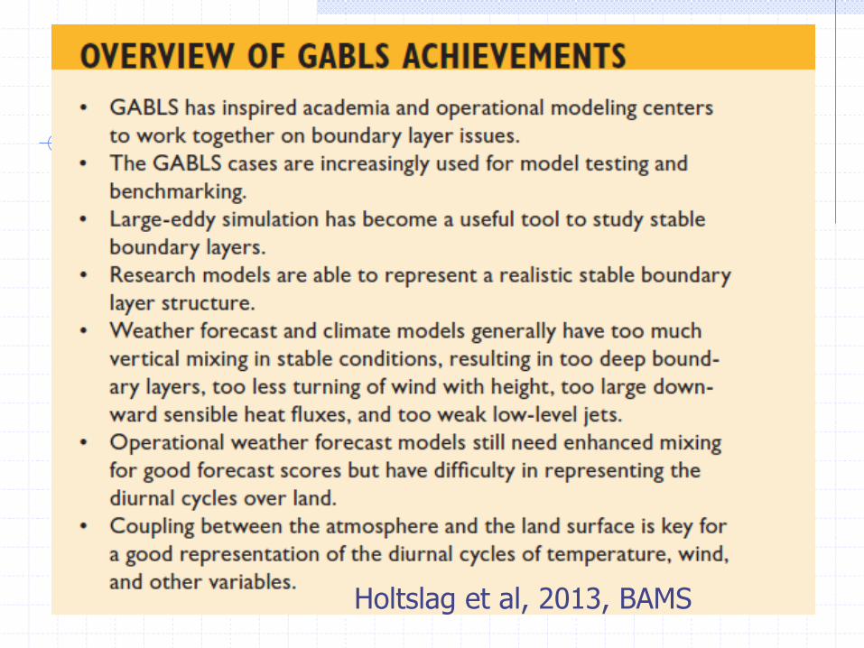
Holtslag et al, 2013, BAMS

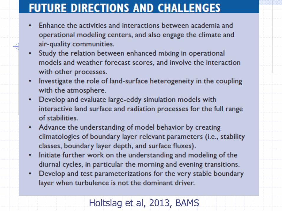
Holtslag et al, 2013, BAMS

56

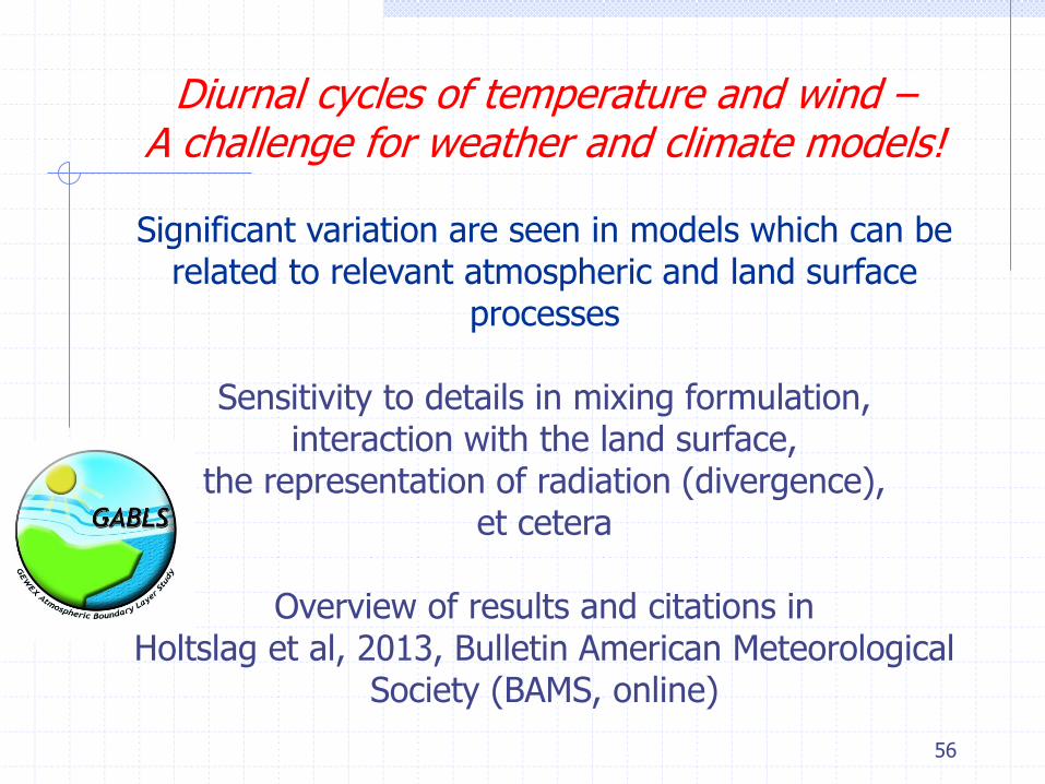
Diurnal cycles of temperature and wind – A challenge for weather and climate models!

Significant variation are seen in models which can be

related to relevant atmospheric and land surface processes

Sensitivity to details in mixing formulation,

interaction with the land surface, the representation of radiation (divergence),

et cetera

Overview of results and citations in Holtslag et al, 2013, Bulletin American Meteorological

Society (BAMS, online)

Helsinki meeting 14/15 Feb 2013

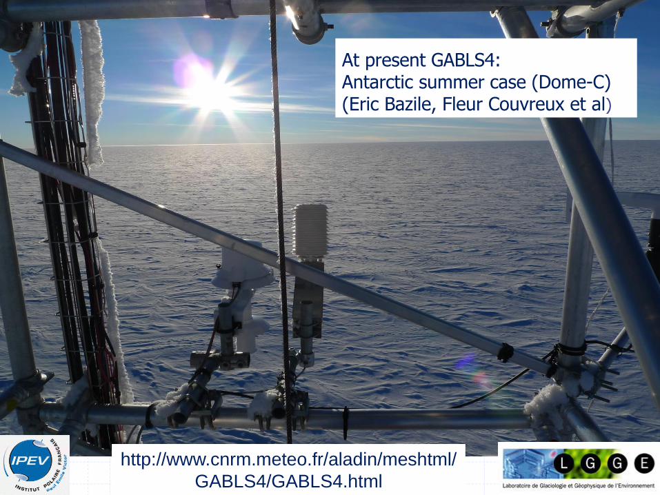
At present GABLS4: Antarctic summer case (Dome-C) (Eric Bazile, Fleur Couvreux et al)

http://www.cnrm.meteo.fr/aladin/meshtml/

GABLS4/GABLS4.html

58

GABLS basic publications (plus many conference and invited presentations)

GABLS1: Special issue Feb 2006, Boundary Layer Meteorology (7 papers) Svensson and Holtslag, 2009, BLM (wind turning issue) GABLS2: Steeneveld et al, 2006, JAS (SCM) and 2008, JAMC (Mesoscale study) Holtslag et al, 2007, BLM (Coupling to land surface) Kumar et al, 2010, JAMC (LES study) Svensson et al, 2011, BLM (SCM intercomparison) GABLS3: Baas et al 2010, QJRMS (set up case and SCM tests) Special issue of BLM 2014, including intercomparison papers by Bosveld et al (2014, SCM), Edwards et al (2014, LES + Radiation).... GABLS overview paper in 2013 (Holtslag et al, BAMS, online)