Embed Size (px)
Citation preview

1
Modulation and Multiplexing
2
Agenda
•Modulation Concept
•Analog Communication
•Digital Communication
•Digital Modulation Schemes
3
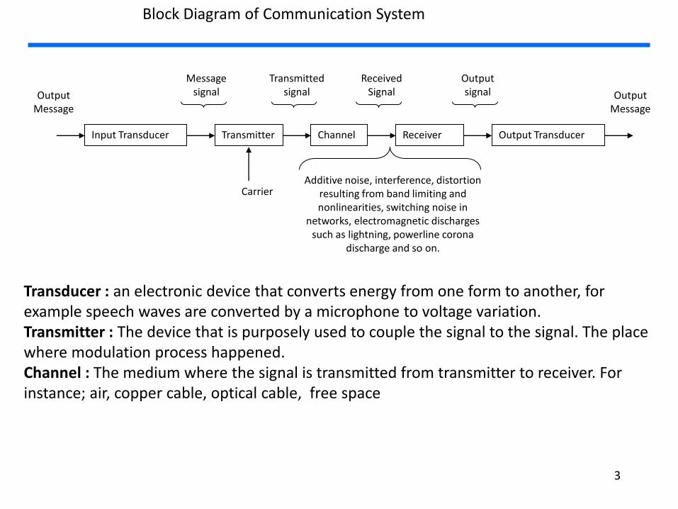
Block Diagram of Communication System
Input Transducer Transmitter Channel Receiver Output Transducer
Message signal
Transmitted signal
Received Signal
Output signal Output
Message Output
Message
Carrier Additive noise, interference, distortion
resulting from band limiting and nonlinearities, switching noise in
networks, electromagnetic discharges such as lightning, powerline corona
discharge and so on.
Transducer : an electronic device that converts energy from one form to another, for example speech waves are converted by a microphone to voltage variation. Transmitter : The device that is purposely used to couple the signal to the signal. The place where modulation process happened. Channel : The medium where the signal is transmitted from transmitter to receiver. For instance; air, copper cable, optical cable, free space
ETM3136 Chapter 2 3 / 69
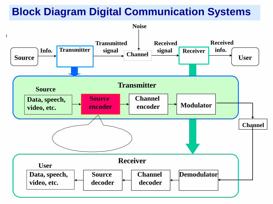
Info. Transmitter Transmitted
signal
Received
signal Receiver
Received
info.
Noise
Channel Source User
Source
encoder
Channel
encoder Modulator
Source
decoder
Channel
decoder
Demodulator
Transmitter
Receiver
Block Diagram Digital Communication Systems
Data, speech,
video, etc.
Data, speech,
video, etc.
Source
User
Channel

5
Modulation

6
Why Modulate Signals? • If we transmit signal through electromagnetic waves, we need
antennas to recover them at a remote point.
• At low frequencies (baseband), the wavelengths are very large. – Ex. Voice, at approx. 4 kHz, has a wavelength of 75 Km!!
• If we “move” those signals to higher frequencies, we can get more manageable antennas.
• After receiving the signal, we need to “move” them back to the original frequency band (baseband) through demodulation.
• Therefore, you can see the modulation task as “giving wings” to the information message.
7
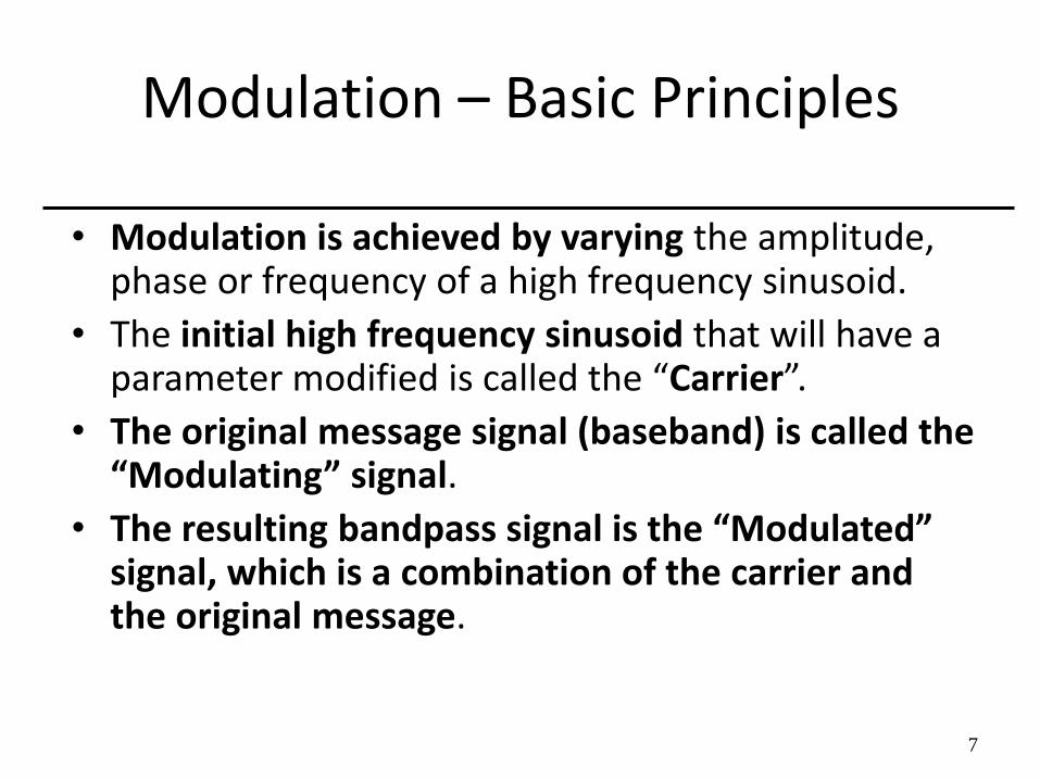
Modulation – Basic Principles
• Modulation is achieved by varying the amplitude, phase or frequency of a high frequency sinusoid.
• The initial high frequency sinusoid that will have a parameter modified is called the “Carrier”.
• The original message signal (baseband) is called the “Modulating” signal.
• The resulting bandpass signal is the “Modulated” signal, which is a combination of the carrier and the original message.

8
Modulation – Basic Principles
Modulating
Signal V(t), at
baseband(fB)
Carrier (fC)
Action on carrier’s
amplitude, frequency
or phase
Modulated Signal
carrying the
information of
V(t), bandpass (fC)
fC
fC

9
MODULATION AND MULTIPLEXING - 1
• MODULATION – THIS IS THE WAY INFORMATION IS
ENCAPSULATED FOR TRANSMISSION
• MULTIPLEXING – THIS IS THE WAY MORE THAN ONE LINK CAN
BE CARRIED OVER A SINGLE COMMUNICATIONS CHANNEL

10
MODULATION AND MULTIPLEXING - 2
Fig. 5.1 in text: (A) At uplink earth station (B) At downlink earth station
11
MODULATION AND MULTIPLEXING - 3
• KEY POINTS – You have to multiplex before modulating on the
transmit side (that is, you have to get all of the output signals together prior to modulating onto a carrier)
– You have to demodulate before demultiplexing on the receive side (that is, before you can separate - i.e. demultiplex - the incoming signals, you have to demodulate the carrier to obtain the transmitted information)

12
Analog Communications

13
ANALOG TELEPHONY - 1
• Baseband voice signal
– 300 - 3400 Hz (CCITT, now called ITU-T)
– 300 - 3100 Hz (Bell) We will use the ITU-T definition
14
ANALOG TELEPHONY - 2
• KEY POINT – THE NUMBER OF VOICE CHANNELS A SATELLITE
TRANSPONDER CAN CARRY VARIES INVERSELY WITH THE AVERAGE POWER LEVEL PER CHANNEL
NOTE:A pessimistic choice (power level set too high)
will lower capacity estimate; An optimistic choice
(power level set too low) can reduce quality of signals
Simple Example

15
CHANNEL LOADING EXAMPLE - 1
A 25 W transponder is designed to carry 250 two-way telephone
channels (giving 500 channels at RF).
Q1. How much power is available for each telephone channel?
Answer: Power per channel = (25) / (500) = 50 mW
Q2. If the amplifier requires to be backed off 3 dB to preserve
linearity, what is the power available per telephone channel now?
Answer: Power per channel = (25/2) / (500) = 25 mW
Q2. What is the power per channel in the second case if 1000 RF
channels are carried?
Answer: Power per channel = (25 mW) / 2 = 12.5 mW

16
SATELLITE ANALOG
• Satellite transponders are bandwidth limited
• A flexible scheme is therefore required for loading analog voice channels
• earth stations may transmit in multiples of 12 voice channels (from 12 to 1872)
NOTE: There is very little analog (FM) voice traffic over satellites
now. The bulk of the high capacity traffic is carried over optical
fibers. The majority of voice capacity is in small digital carriers
called IDR (Intermediate Digital Rate)
17
FREQUENCY MODULATION - 1
• DEFINITION “Frequency modulation results when the deviation, f, of the instantaneous frequency, f, from the carrier frequency fc is directly proportional to the instantaneous amplitude of the modulating voltage”.
LET’S LOOK AT THIS PICTORIALLY
18
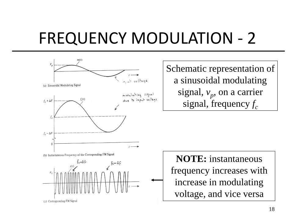
FREQUENCY MODULATION - 2
Schematic representation of
a sinusoidal modulating
signal, vp, on a carrier
signal, frequency fc
NOTE: instantaneous
frequency increases with
increase in modulating
voltage, and vice versa
19
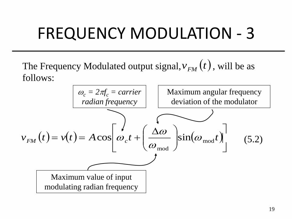
FREQUENCY MODULATION - 3
The Frequency Modulated output signal, , will be as
follows:
(5.2)
tvFM
ttAtvtv cFM mod
mod
sincos
Maximum angular frequency
deviation of the modulator
c = 2fc = carrier
radian frequency
Maximum value of input
modulating radian frequency

20
CARSON’S RULE - 1 Carson’s rule states that the transmission bandwidth, BT,
is given by: mod2 fB f
Where B is the bandwidth of the modulating signal
which, for a sinusoidal modulating signal, is the highest
modulating frequency, fmod.
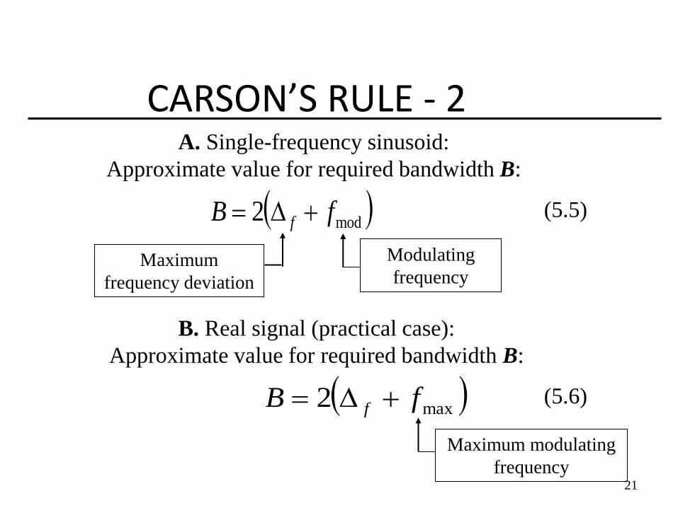
21
CARSON’S RULE - 2 A. Single-frequency sinusoid:
Approximate value for required bandwidth B:
(5.5)
Maximum
frequency deviation
Modulating
frequency
B. Real signal (practical case):
Approximate value for required bandwidth B:
max2 fB f (5.6)
Maximum modulating
frequency
mod2 fB f

22
FM IMPROVEMENT • FM modulation is relatively inefficient with the use of
transmission spectrum
– A small baseband bandwidth is converted into a large RF bandwidth
• FM demodulation and detection converts the wide RF bandwidth occupied into a small baseband bandwidth occupied
– Ratio of RF to baseband bandwidths gives an improvement in signal to noise ratio which leads to the so-called FM IMPROVEMENT
23
Digital Communications
24
DIGITAL COMMUNICATIONS -1
• Many signals originate in digital form – data from computers
– data from digital fixed and mobile systems
– digitized information (e.g. voice)
• World-wide network is moving towards all-digital system
• Computers can only handle digital signals

25
Why Digital Transmission? • Robustness
– Generally less susceptible to degradations
– But...when it does degrade tends to fail quickly
• Adaptiveness – Can easily combine a mix of signal information
• Data, voice, video, multiple user signals
• Compatibility - with digital storage, etc.
• Security - not easily received except by recipient

26
DIGITAL COMMUNICATIONS -2
• At baseband, send V (volts) to represent a logical 1 and 0
• At RF - digitally modulate the carrier
– ASK Amplitude Shift Keying
– FSK Frequency Shift Keying
– PSK Phase Shift Keying
• Binary forms of these are OOK, BFSK, and BPSK, respectively
Let’s first look at basic Digital Communications from
the book by COUCH (7th. Edition)
Outline ƒ Baseband Pulse Transmission
ƒ Line Coding
Line Coding • How do we produce the physical waveform of a digital signal?
• Binary 1’s and 0’s, such as in PCM signalling, may be represented
in various serial-bit signalling formats called line codes.
• Line codes are also used for controlling and shaping the power
spectral density of a digital communication signal so that the
spectrum of the transmitted signal matches the spectral
characteristics of a baseband or equivalent lowpass channel.
• Choosing the appropriate line code can minimise the effect of
channel distortion and noise in transmission.
• There are two major categories: return-to-zero (RZ) and nonreturn-
to-zero (NRZ).
• With RZ coding, the waveform returns to a zero-volt level for a
portion (usually one-half) of the bit interval.

Binary Line Codes • Unipolar Signaling : binary 1 is represented by a high level (+A
volts) and a binary 0 by a zero level; also called on-off keying.
• Polar Signaling : binary 1’s and 0’s are represented by equal
positive and negative levels.
• Bipolar Signaling : binary 1’s are represented by alternately
positive or negative values. The binary 0 is represented by a zero
level, also called alternate mark inversion (AMI) signaling.
• Manchester Signaling : each binary 1 is represented by a
positive half-bit period pulse followed by a negative half-bit
period pulse while a binary 0 is represented by a negative half-bit
period pulse followed by a positive half-bit period pulse. Also
called split-phase encoding.

Desirable Properties of Line Codes • Self-synchronisation: There is enough timing information built
into the code so that bit synchronizers can be designed to extract
the timing or clock signal.
• Low probability of bit error: Receivers can be designed that will
recover the binary data with a low probability of bit error when
the signal is corrupted by noise or ISI.
• A spectrum that is suitable for the channel
• Transmission bandwidth: This should be as small as possible
• Error detection capability: It should be possible to implement
channel coding techniques. • Transparency: The data protocol and line code are designed so
that every possible sequence of data can be transmitted and
received.

Intersymbol Interference

Intersymbol Interference • Digital data have broad spectrum with significant low-freq. content.
• Digital baseband transmission requires a lowpass channel with a
bandwidth sufficient to accommodate the essential frequency
content of the data stream.
• If these pulses are transmitted across a bandlimited channel, they
will spread in time and smear into adjacent time slots and cause
intersymbol interference (ISI).
• ISI is a major source of bit errors in the receiver. To correct it,
control has to be exercised over the pulse shape in the overall
system. Another approach to mitigate ISI is to equip the receiver
with an equaliser.

Intersymbol Interference
rk=sk+nk+
∑αisi
i≠k
• We can restrict the signal bandwidth by using pulses with rounded
tops (instead of flat tops).
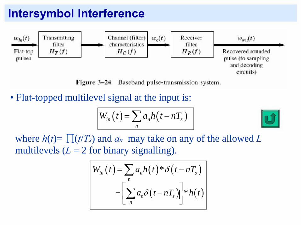
Intersymbol Interference
• Flat-topped multilevel signal at the input is:
where h(t)= ∏(t/Ts) and an may take on any of the allowed L
multilevels (L = 2 for binary signalling).
in n s
n
W t a h t nT
*in n s
n
W t a h t t nT
*n s
n
a t nT h t
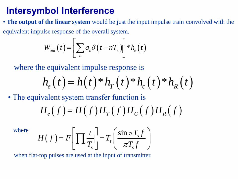
Intersymbol Interference • The output of the linear system would be just the input impulse train convolved with the
equivalent impulse response of the overall system.
where the equivalent impulse response is
• The equivalent system transfer function is
where
when flat-top pulses are used at the input of transmitter.
*out n s e
n
W t a t nT h t
* * *e T c Rh t h t h t h t h t
e T C RH f H f H f H f H f
sin s
s
s s
T ftH f F T
T T f
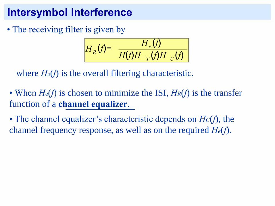
Intersymbol Interference • The receiving filter is given by
H
R
H
(f)=
e
(f) H(f)H
T
(f)H
C
(f)
where He(f) is the overall filtering characteristic.
• When He(f) is chosen to minimize the ISI, HR(f) is the transfer
function of a channel equalizer.
• The channel equalizer’s characteristic depends on HC(f), the
channel frequency response, as well as on the required He(f).
Nyquist’s Method

Pulse Shaping to Reduce ISI: Nyquist’s First Method • Nyquist’s first method for eliminating ISI is to use an equivalent
transfer function, He(f), such that the impulse response satisfies the
condition.
⎧C, k=0
⎨ ⎩
0, k≠0
where k is an integer, Ts is the symbol (sample) clocking period, τ is
the offset in the receiver sampling clock times compared with the
clock times of the input symbols, and C is a nonzero constant.
• It means that for a single flat-top pulse of level a present at the input
to transmitting filter at t = 0, the received pulse would be a C at t = τ
but would not cause interference at other sampling times because
he(kTs + τ) = 0 for k ≠ 0.
e sh kT
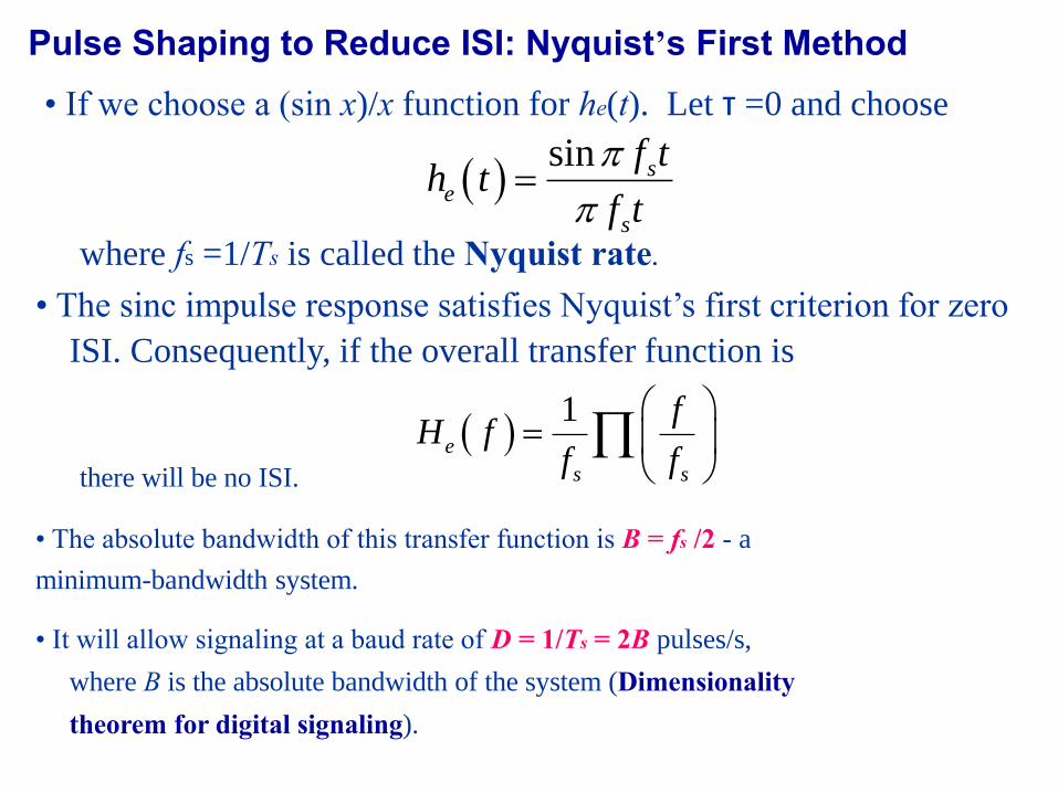
Pulse Shaping to Reduce ISI: Nyquist’s First Method • If we choose a (sin x)/x function for he(t). Let τ =0 and choose
where fs =1/Ts is called the Nyquist rate.
• The sinc impulse response satisfies Nyquist’s first criterion for zero ISI. Consequently, if the overall transfer function is
there will be no ISI.
• The absolute bandwidth of this transfer function is B = fs /2 - a
minimum-bandwidth system.
• It will allow signaling at a baud rate of D = 1/Ts = 2B pulses/s,
where B is the absolute bandwidth of the system (Dimensionality
theorem for digital signaling).
sin s
e
s
f th t
f t
1
e
s s
fH f
f f

Pulse Shaping to Reduce ISI: Nyquist’s First Method
(a) System’s ideal Nyquist spectrum P(f ) = 1/(2W) • rect[ f / (2W)]
(b) Ideal shaped sinc pulse at system output p(t) = sinc(2Wt)
Tb = 1/(2W)
∴ Rb= 2W
= min. Nyquist bandwidth
W
(a) Ideal magnitude response.
(b) Ideal basic pulse shape.

Pulse Shaping to Reduce ISI: Nyquist’s First Method
Binary sequence 1
0
1
1
0
1
0
1
0.8
0.6
0.4
0.2
0
-0.2
-0.4
-0.6
-0.8
-1
-2
-1
0
1
2
3
4
5
6
7
8
9
10
Time
A series of sinc pulses corresponding to the sequence 1011010

Pulse Shaping to Reduce ISI: Nyquist’s First Method • The sinc type of overall pulse shape has two practical difficulties:
™ The overall amplitude transfer characteristic He(f) has to be flat over -
B < f < B and zero elsewhere. This is unrealizable as the impulse
response is noncausal and of infinite duration.
™ The synchronization of the clock in the decoding sampling circuit has
to be almost perfect, since the sinc pulse decays only as 1/x and is zero
in adjacent time slots only when t is at the exact sampling instant.
Inaccurate sync will cause considerable ISI.
• Because of these problems, we should consider other pulse shapes
that have a slightly wider bandwidth.
• Solution: find pulse shapes that go through zero at adjacent
sampling points and yet have an envelope that decays much faster
than 1/x, one example is the raised cosine-rolloff Nyquist filter.
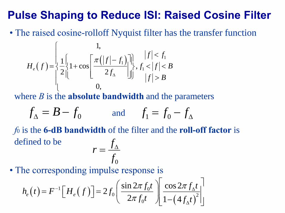
Pulse Shaping to Reduce ISI: Raised Cosine Filter • The raised cosine-rolloff Nyquist filter has the transfer function
where B is the absolute bandwidth and the parameters
and
f0 is the 6-dB bandwidth of the filter and the roll-off factor is
defined to be
• The corresponding impulse response is
1
1
1
1,
11 cos ,
2 2
0,
e
f ff f
H f f f Bf
f B
0f B f 1 0f f f
0
fr
f
1 00 2
0
sin 2 cos 22
2 1 4e e
f t f th t F H f f
f t f t

Pulse Shaping to Reduce ISI: Raised Cosine Filter

Pulse Shaping to Reduce ISI: Raised Cosine Filter
Pulse Shaping to Reduce ISI: Raised Cosine Filter • As the absolute bandwidth is increased (e.g., r = 0.5 or r = 1.0) :
1. The filtering requirements are relaxed, although he(t) is still
noncausal
2. The clock timing requirements are relaxed also, since the
envelope of the impulse response decays faster than 1/|t|(on
the order of 1/|t|³ for large values of t).
• To determine the baud rate that can be supported by the raised
cosine-rollof system, note that the data pulses can be inserted at t =
n/2f0 where n ≠ 0. Therefore, baud rate, D = 1/Ts = 2f0.
• In other words, the 6-dB bandwidth of the raised cosine-rolloff
filter, f0 is designed to be half the symbol (baud) rate.

Pulse Shaping to Reduce ISI: Raised Cosine Filter • The transmission bandwidth is defined by
B= f
0
+ f
∆
= f
0
+ rf
0
=(1+r)f
0
• However, the filter is noncausal. We can introduce a delay of Td
sec, this would move the peak of the impulse response to the right
(along the time axis), and then the filter would be approximately
causal.
• Goals and trade-off in pulse-shaping
‰ Reduce ISI
‰ Efficient bandwidth utilization
‰ Robustness to timing error (small side lobes)

Adaptive Equalizer

Equalization to Reduce ISI • ISI due to filtering effect of the communications channel (e.g. wireless channels) ƒ Channels behave like band-limited filters
H
c (f)=H
c
jθ
(f)e
c
(f)
Non-constant amplitude
Non-linear phase
Amplitude distortion
Phase distortion
ƒ Equalization is a technique to remove ISI caused by the
channel
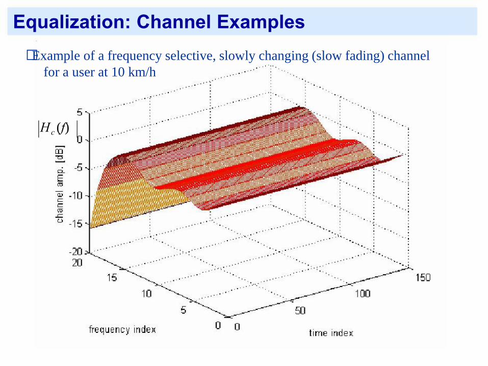
Equalization: Channel Examples
ƒ Example of a frequency selective, slowly changing (slow fading) channel
for a user at 10 km/h
H
c (f)
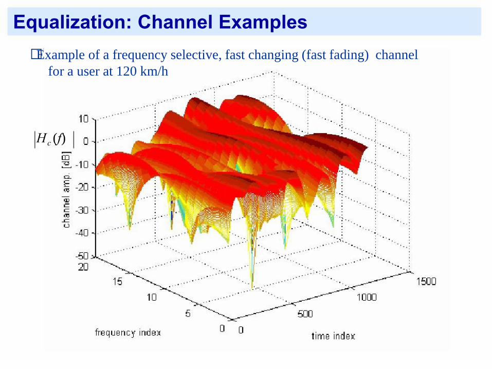
Equalization: Channel Examples
ƒ Example of a frequency selective, fast changing (fast fading) channel
for a user at 120 km/h
H
c (f)
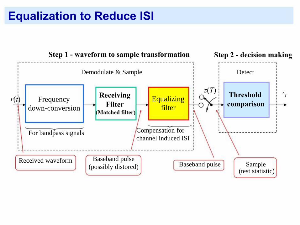
Equalization to Reduce ISI
Step 1 - waveform to sample transformation
Demodulate & Sample
Step 2 - decision making
Detect
z(T) r(t) Frequency
down-conversion
For bandpass signals
Receiving Filter
(Matched filter)
Equalizing
filter
Compensation for
channel induced ISI
Threshold ˆi
comparison
Received waveform
Baseband pulse
(possibly distored)
Baseband pulse Sample (test statistic)
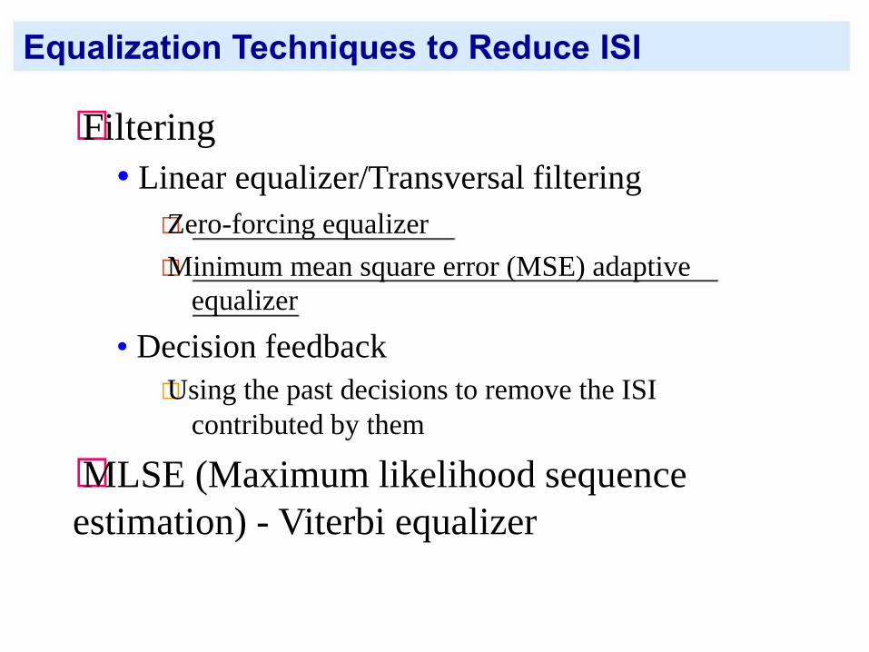
Equalization Techniques to Reduce ISI
ƒ Filtering • Linear equalizer/Transversal filtering
‰ Zero-forcing equalizer
‰ Minimum mean square error (MSE) adaptive
equalizer • Decision feedback
‰ Using the past decisions to remove the ISI
contributed by them
ƒ MLSE (Maximum likelihood sequence
estimation) - Viterbi equalizer

Equalization by Transversal Filtering • The principle of a linear equalizer/transversal filter is very
simple: Apply a filter E(z) at the receiver, mitigating the effect
of ISI.

Equalization by Transversal Filtering • Transversal filter: - A weighted tap delayed line that reduces the effect of ISI
by proper adjustment of the filter taps.
N z(t)= c x(t
−n ) n=−N ,..., N k
=−2N,...,2N
x(t)
∑ n=−N
n
c− c
c c
N −N+1
N−1 N
∑ z
Coeff.
adjustment
(t)

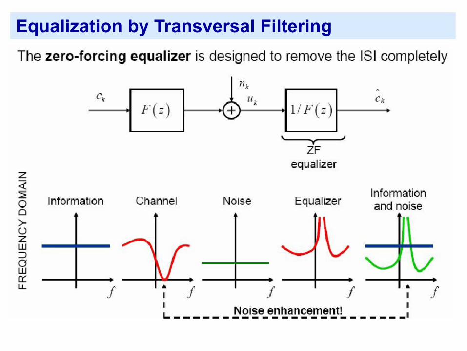
Equalization by Transversal Filtering • Zero-forcing equalizer: - The filter taps are adjusted such that the equalizer output is
forced to be zero at N sample points on each side:
Adjust
z(k)=
⎧1 k=0
⎨
{c }
n n=−N
0 ⎩
k=±1,...,±N
• Mean Square Error (MSE) equalizer: - The filter taps are adjusted such that the MSE of ISI and noise
power at the equalizer output is minimized.
Adjust
minE[(z(kT)−
2
a )
]
{c
N k }
n
n=
−
N
N
Equalization by Transversal Filtering
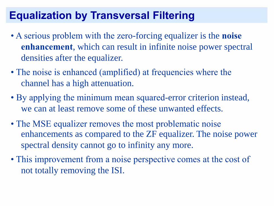
Equalization by Transversal Filtering • A serious problem with the zero-forcing equalizer is the noise
enhancement, which can result in infinite noise power spectral
densities after the equalizer.
• The noise is enhanced (amplified) at frequencies where the
channel has a high attenuation.
• By applying the minimum mean squared-error criterion instead,
we can at least remove some of these unwanted effects.
• The MSE equalizer removes the most problematic noise
enhancements as compared to the ZF equalizer. The noise power
spectral density cannot go to infinity any more.
• This improvement from a noise perspective comes at the cost of
not totally removing the ISI.

Equalization by Transversal Filtering

Decision-Feedback Equalizer • The idea is to subtract the interference caused by already detected
data (symbols) through a feedback filter.
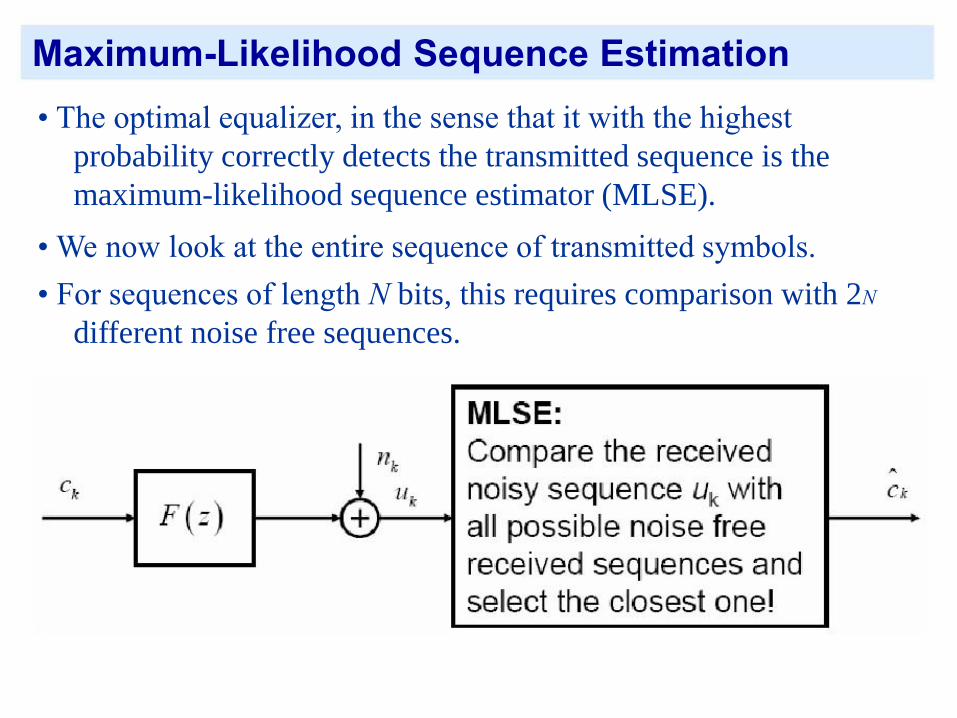
Maximum-Likelihood Sequence Estimation • The optimal equalizer, in the sense that it with the highest
probability correctly detects the transmitted sequence is the
maximum-likelihood sequence estimator (MLSE).
• We now look at the entire sequence of transmitted symbols.
• For sequences of length N bits, this requires comparison with 2N
different noise free sequences.

Maximum-Likelihood Sequence Estimation • This equalizer seems over-complicated and too complex.
• The discrete-time channel F(z) is very similar to the convolution
encoder, but with here complex input/output and rate 1:
• We can build a trellis and use the Viterbi algorithm to
efficiently calculate the best path!

Maximum-Likelihood Sequence Estimation • The Viterbi-equalizer (detector) is optimal in terms of minimizing
the probability of detecting the wrong sequence of symbols.
• For transmitted sequences of length N over a length L+1 channel,
it reduces the brute-force maximum-likelihood detection
complexity of 2N comparisons to N stages of 2L comparisons
through elimination of trellis paths. L is typically MUCH
SMALLER than N.
• Even if it reduces the complexity considerably (compared to brut-
force ML) it can have a too high complexity for practical
implementations if the length of the channel (ISI) is large.
• In GSM there is a known training sequence transmitted in every
burst, which is used to estimate the channel so that a Viterbi-
equalizer can be used to remove ISI.

Summary of Channel Equalizers • Linear equalizers suffer from noise enhancement.
• Decision-feedback equalizers (DFEs) use decisions on data to
remove parts of the ISI, allowing the linear equalizer part to be
less ”powerful” and thereby suffer less from noise enhancement.
• Incorrect decisions can cause error-propagation in DFEs, since an
incorrect decision may add ISI instead of removing it.
• Maximum-likelihood sequence estimation (MLSE) is optimal
in the sense of having the lowest probability of detecting the
wrong sequence.
• Brute-force MLSE is prohibitively complex.
• The Viterbi-eualizer (detector) implements the MLSE with
considerably lower complexity.

Analog Data, Data Signal
• Analog to Digital Conversion (ADC) method is:
– Pulse Code Modulation
– Differential Pulse Code Modulation
– Delta Modulation
• The ADC process can also be called Digital Pulse Modulation
DEPARTMENT OF ELECTRICAL, ELECTRONICS & SYSTEMS ENGINEERING
UNIVERSITI KEBANGSAAN MALAYSIA

Pulse Modulation
• Pulse modulation used the sampling technique.
– The first operation is the conversion of analog to digital:
• Sampling the analog signal with certain duration.
• Representing the signal in pulses form
• The sided pulses have the same distance/duration.
DEPARTMENT OF ELECTRICAL, ELECTRONICS & SYSTEMS ENGINEERING
UNIVERSITI KEBANGSAAN MALAYSIA

Pulse Modulation
(a)Naturally sampling (b) Flat topped sampling
utilizing ‘sample &
hold’circuit

Sampling
• Nyquist Sampling Theorem for bounded signal with infinite energy is:
– Bounded band signal (width W Hz) is repeated for every 2W Hz or 1/2W second. (Transmitter)
– Bounded band signal (width W Hz) can be re- shaped at receiver if we know the sampling is taken at Ts=1/2W second. (receiver)
PAM Sampling Quantization Encoder
Low pass Filter
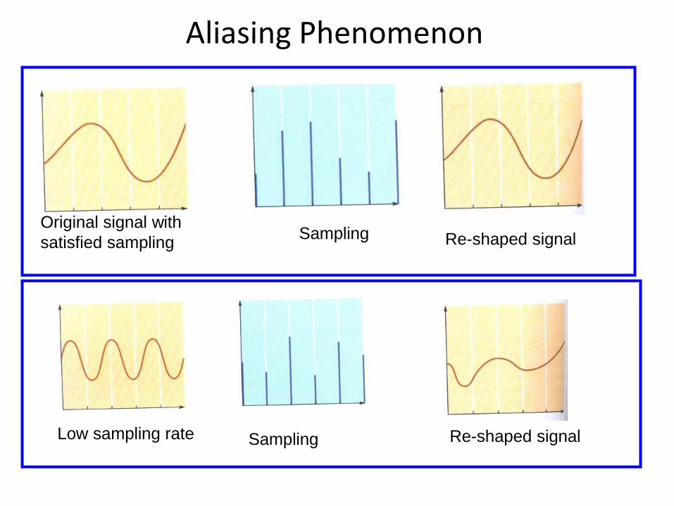
Aliasing Phenomenon
Low sampling rate Sampling Re-shaped signal
Re-shaped signal Sampling Original signal with
satisfied sampling
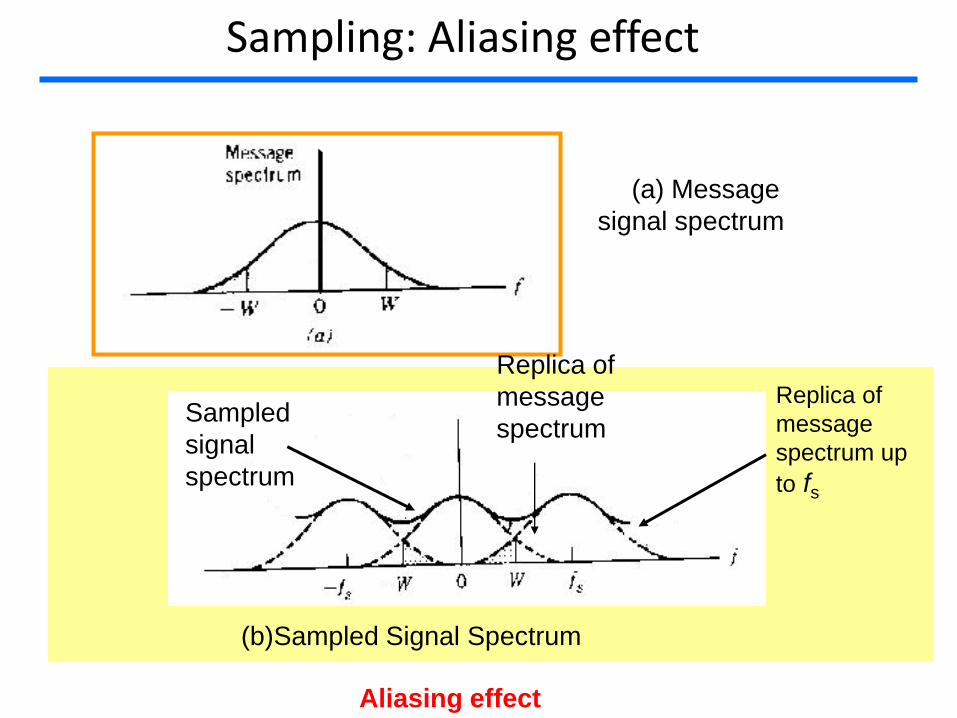
Sampling: Aliasing effect
(a) Message
signal spectrum
(b)Sampled Signal Spectrum
Sampled
signal
spectrum
Replica of
message
spectrum
Replica of
message
spectrum up
to fs
Aliasing effect
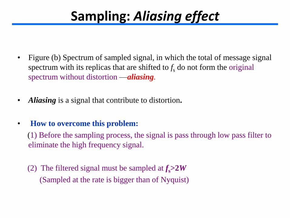
Sampling: Aliasing effect
• Figure (b) Spectrum of sampled signal, in which the total of message signal
spectrum with its replicas that are shifted to fs do not form the original
spectrum without distortion —aliasing.
• Aliasing is a signal that contribute to distortion.
• How to overcome this problem:
(1) Before the sampling process, the signal is pass through low pass filter to
eliminate the high frequency signal.
(2) The filtered signal must be sampled at fs>2W
(Sampled at the rate is bigger than of Nyquist)
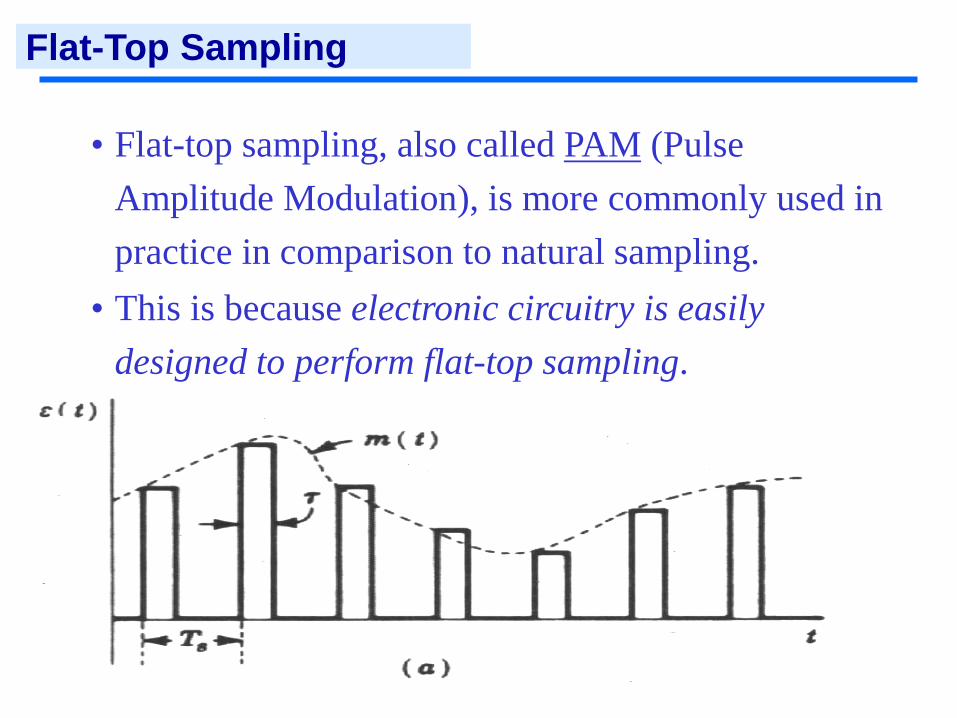
• Flat-top sampling, also called PAM (Pulse
Amplitude Modulation), is more commonly used in
practice in comparison to natural sampling.
• This is because electronic circuitry is easily
designed to perform flat-top sampling.
• The top of a flat-top sampled pulse is flat.
Flat-Top Sampling

Pulse Amplitude Modulation
• Pulse modulation based on the sampling theorem
• The pulse amplitude is change according to the analog
signal.
1.8 2.0
5.6 5.4
3.1
6.2
Ts=1/2W s Pulse of Pulse amplitude Modulation (PAM)

Analog Pulse Modulation technique
(a) Original signal (b) PAM signal
(c) Pulse Duration Modulation (PDM) signal (d) Pulse Position Modulation (PPM) Signal

Analog Pulse Modulation technique
(c) Pulse Duration Modulation (PDM) signal (d) Pulse Position Modulation (PPM) Signal
Pulse Time Modulation: Pulse Width Modulation and Pulse
Position Modulation
• Pulse time modulation (PTM) is a class of signalling techniques that encodes the sample values of an analog signal onto the time axis of a digital signal.
• The two main types of PTM are:
Pulse width modulation (PWM): also called pulse duration
modulation (PDM), where sample values of the analog waveform
are used to determine the width of the pulse signal.
Pulse position modulation (PPM): the analog sample value
determines the position of a narrow pulse relative to the clocking
time.

Pulse Code Modulation
Sampling Quantisation Encoding
analogue
signal
digital
signal
• PCM (Pulse Code Modulation) is an analogue-to-digital
conversion process.
• It consists of sampling, quantisation, and encoding.

Sampling
Sampling Quantisation Encoding
PCM Process
samples ms(t) analogue m(t)
• The first stage in PCM is the sampling process.
• Sampling converts an analogue signal to a sequence of
pulses, which have the same amplitudes as their analogue
segments.
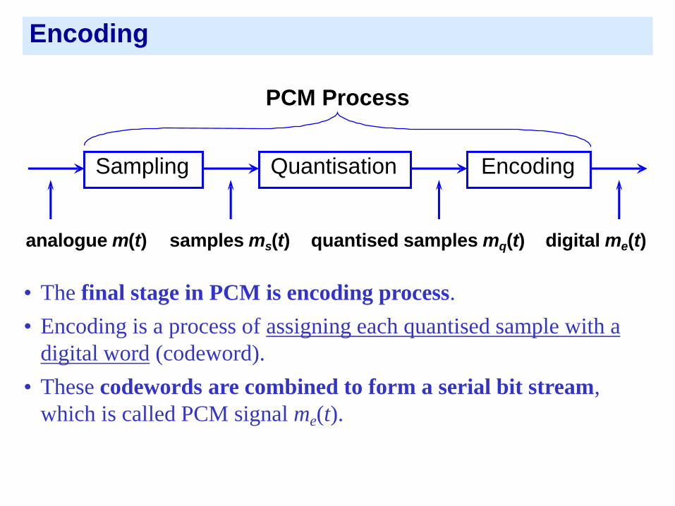
Encoding
Sampling Quantisation Encoding
PCM Process
• The final stage in PCM is encoding process.
• Encoding is a process of assigning each quantised sample with a
digital word (codeword).
• These codewords are combined to form a serial bit stream,
which is called PCM signal me(t).
samples ms(t) quantised samples mq(t) digital me(t) analogue m(t)
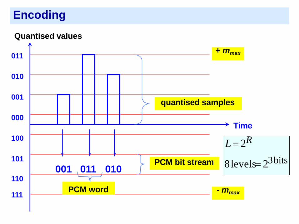
Quantised values
011
010
001
000
100
101
001 011 010 110
quantised samples
PCM bit stream
Time
+ mmax
- mmax 111
L 2R
8levels 23bits
PCM word
Encoding

Pulse Code Modulation (PCM)
• Very frequently used in Digital Communication.
• The signal voltage is divided into several levels.
• Each of the level is assigned a binary number.
• N= number of levels
• m= bits in one sample
2mN
Example: PCM
• Find the number of level if number of bit per sample are:
(a) 8 (telephone)
(b) 16 (CD)

Example: PCM
• Find the number of level if number of bit per sample are:
(a) 8 (telephone)
(b) 16 (CD)
Solution: (a) N=28=256 levels
(b) N=216=65,536 levels

Analog input signal
(Time Continuous)
Amplitude
Signal PCM Pulse
Pulse Code Modulation (PCM)
Digital output signal
(bit sequence)
PCM system fundamental element
(a) Transmitter section
PAM Sampling Quantization Encoder
Lowpass filter

Advantages & Disadvantages of PCM
Advantages
•PCM digital circuitry is inexpensive.
•PCM signals may be multiplexed with other digital signals, and
transmitted over a common channel.
•The noise performance of PCM digital systems is superior.
Disadvantages
•A much wider transmission bandwidth is needed by a PCM digital
signal compared to its analogue signal.
•Recovered analogue signals contain quantising errors.
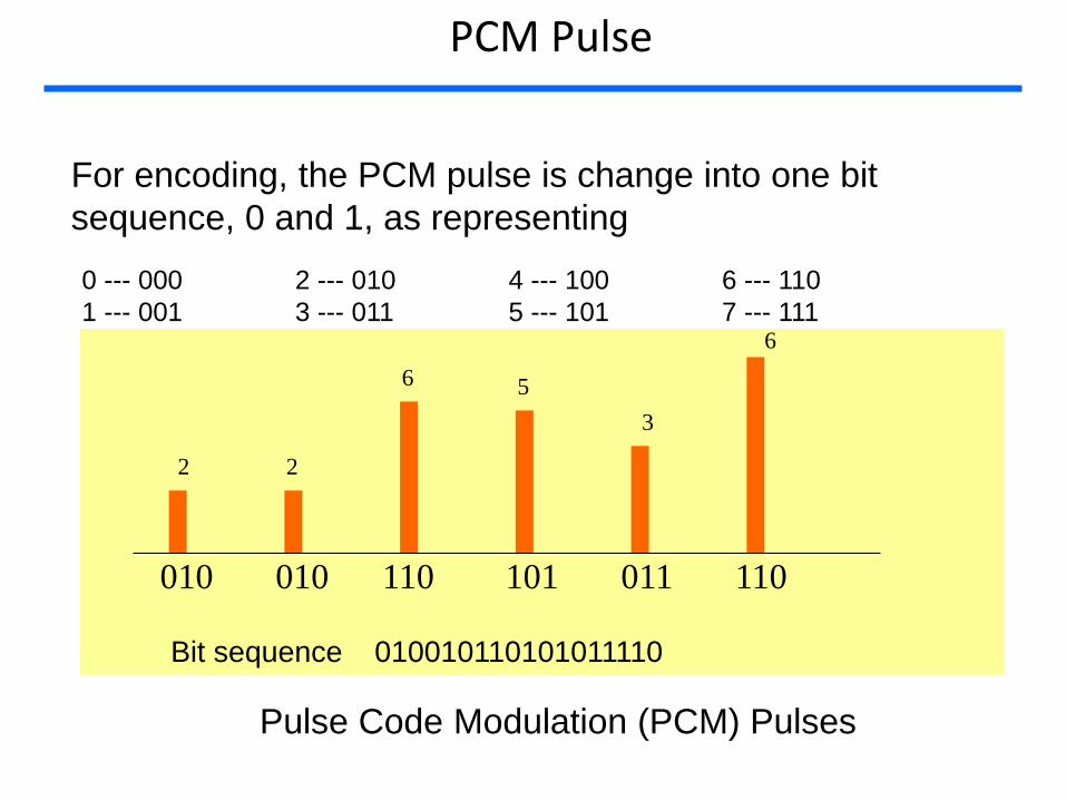
PCM Pulse
Pulse Code Modulation (PCM) Pulses
Bit sequence 010010110101011110
2 2
6 5
3
6
010 010 110 101 011 110
For encoding, the PCM pulse is change into one bit
sequence, 0 and 1, as representing
0 --- 000 2 --- 010 4 --- 100 6 --- 110
1 --- 001 3 --- 011 5 --- 101 7 --- 111

Quantised values
011
010
001
000
100
101
001 011 010 110
quantised samples
PCM bit stream
Time
+ mmax
- mmax 111
L 2R
8levels 23bits
PCM word
Encoding

Quantization
• Continuous-time signal such as voice signal has the continuous amplitude range.
• Therefore, the samples also have
– Continuous amplitude range and
– not compulsory to be sent with the original amplitude.
PAM sampling Quantization Encoder
Lowpass filter

PCM Quantization Method
• The Amplitude of PAM pulse is approximating by the n
integer bit.
• For example, n in PAM diagram is n = 3, therefore 23= 8 level are needed to represent PCM pulse.
• The amplitude of each PAM pulse must be in integer value.
Quantization
Quantization
• Human ear (natural receiver) is not sensitive accurately to the signal.
• The conversion of sampled analog signal to sampled digital signal is called Quantization

Quantization principle: Quantized signal and quantized error (the
different between the Quantized input signal and Quantized
output signal)
Quantization

36 Chapter 2 54
Process Summary of PCM Systems

Quantization Error
• Occurs when the original signal has the infinite number of levels
– Adding the sampling bit number
• The difference between the strongest signal and weakest signal that can be detected.
(1.76 6.02 )Dynamic range m dB
Delta Modulation
• DM is an analog-to-digital signal conversion technique used for transmission of voice information where quality is not of primary importance.
• DM is the simplest form of differential pulse-code modulation (DPCM) where the difference between successive samples is encoded into n-bit data streams.
• In delta modulation, the transmitted data is reduced to a 1 bit data stream.
• To achieve high signal-to-noise ratio, delta modulation must use
oversampling techniques, that is, the analog signal is sampled at a rate several times higher than the Nyquist rate.
Delta Modulation
• The alternative method to PCM in converting the analog signal to digital signal.
• The analog input signal is approximating in step function is up and down.
• The instantaneous value of analog input and step value for every sample is compared.
• The sampling rate is higher because one bit/sample is used
only.
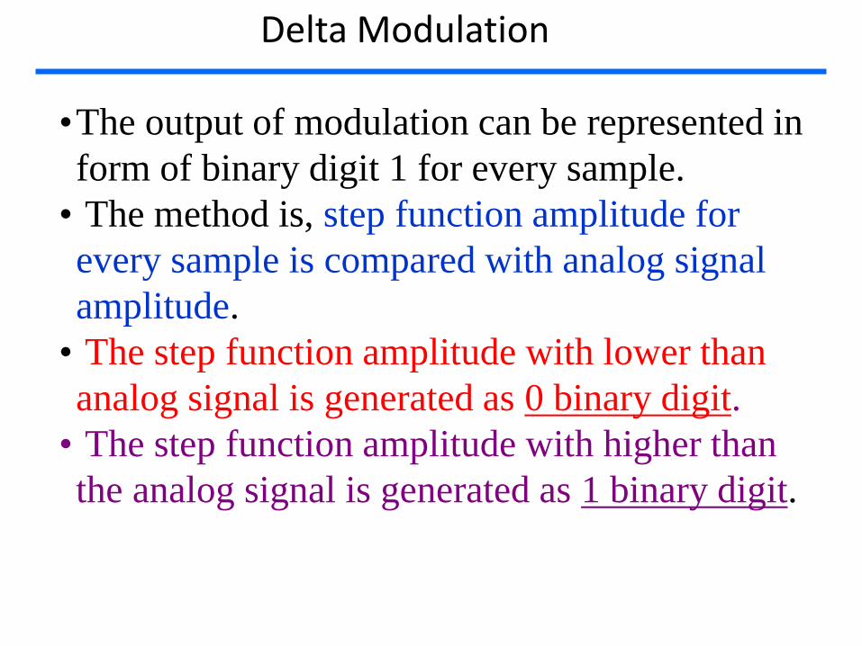
•The output of modulation can be represented in
form of binary digit 1 for every sample.
• The method is, step function amplitude for
every sample is compared with analog signal
amplitude.
• The step function amplitude with lower than
analog signal is generated as 0 binary digit.
• The step function amplitude with higher than
the analog signal is generated as 1 binary digit.
Delta Modulation

• The main attractions of DM are simplicity and low cost.
• DM is attained by using a sampling rate far in excess of that needed
for PCM. The price paid for this benefit is a corresponding increase
in the transmission and therefore channel bandwidth.
• Therefore DM is not suitable for applications where channel
bandwidth is at a premium.
• Delta modulation is subject to two types of quantization error:
(1) slope overload distortion
(2) granular noise
Delta Modulation
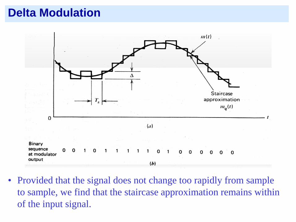
• Provided that the signal does not change too rapidly from sample
to sample, we find that the staircase approximation remains within
of the input signal.
Delta Modulation

Delta Modulation

Granular Noise and Slope Overload Noise in DM
• Slope overload noise occurs when the step size ∆ is too small for the
accumulator output to follow quick changes in the input waveform.
• In other words, the message signal m(t) has a slope greater than can
be followed by the staircase approximation mq(t).
• The maximum slope that can be followed by mq(t) is ∆/Ts.

Delta Modulation
• The significant parameters in Delta Modulation are:
– Step size ,
– Sampling rate (sample/second)
• Step size need to be right chosen for reducing the quantization error
DEPARTMENT OF ELECTRICAL, ELECTRONICS & SYSTEMS ENGINEERING
UNIVERSITI KEBANGSAAN MALAYSIA
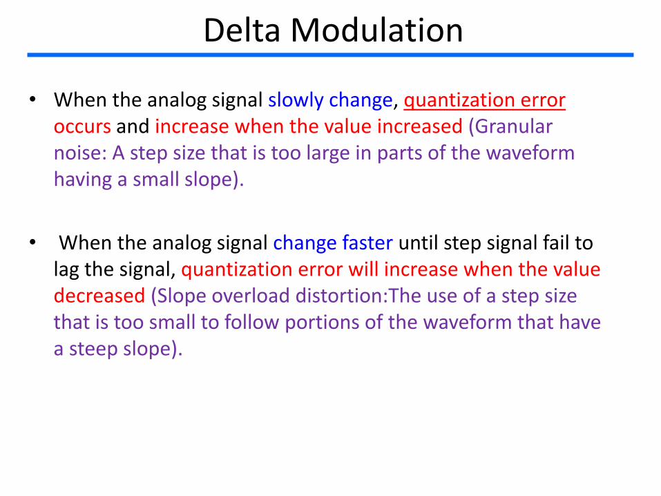
• When the analog signal slowly change, quantization error occurs and increase when the value increased (Granular noise: A step size that is too large in parts of the waveform having a small slope).
• When the analog signal change faster until step signal fail to lag the signal, quantization error will increase when the value decreased (Slope overload distortion:The use of a step size that is too small to follow portions of the waveform that have a steep slope).
Delta Modulation

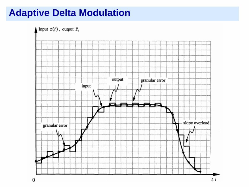
• The choice of the optimum step size ∆ is the result of a
compromise between slope-overload distortion and granular
noise.
• To satisfy such a requirement, we need to make the DM adaptive,
in the sense that the step size is made to vary according to the
input signal. This is called adaptive DM (ADM).
• The underlying principle of all ADM algorithms is two fold:
If DM pulses consist of a string of pulses with the opposite
polarity, then the DM is operating in its granular mode; in this
case, it may be advantageous to reduce the step size ∆.
If successive pulses are of the same polarity, then the delta
modulator is operating in its slope-overload mode; in this
second case, the step size ∆ should be increased.
Adaptive Delta Modulation
Chapter 2
Adaptive Delta Modulation

Conclusion
• The digital technique transmission is vastly used as compared to the analog transmission because of its advantages.
• The analog signal which used the digital scheme need to be convert to digital form—ADC.
• The method that always be used is Pulse Code Modulation (PCM) and Delta Modulation (DM).

Conclusion
• In DM, the selection of step size and sampling rate fs is important for reducing the quantization error.
• The precision of DM technique can be improved by
– Increase the sampling rate but
– It will increase the output signal data rate simultaneously.

Lecture Frame
• Introduction
• ASK- Amplitude Shift Keying
• FSK- Frequency Shift Keying
• PSK- Phase Shift Keying
• QAM- Quadrature Amplitude Modulation
• CPM- Continous Phase Modulation
• MSK- Minimum Shift Keying
• Application of Digital Modulation

Introduction
• The analog signal transmission which modulated digitally between two communication systems, or can be called digital radio system.
• The trend today: The analog modulation system (e.g AM, FM) is replaced by modern digital modulation system that has many advantages as compared to analog modulation.
Introduction
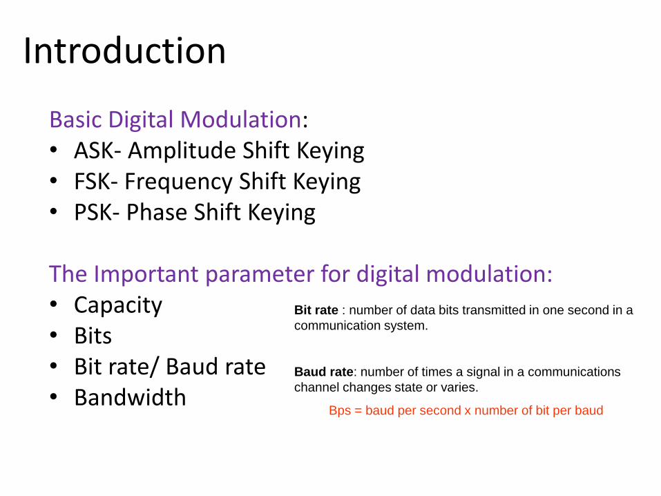
Basic Digital Modulation: • ASK- Amplitude Shift Keying • FSK- Frequency Shift Keying • PSK- Phase Shift Keying The Important parameter for digital modulation: • Capacity • Bits • Bit rate/ Baud rate • Bandwidth
Bit rate : number of data bits transmitted in one second in a
communication system.
Baud rate: number of times a signal in a communications
channel changes state or varies.
Bps = baud per second x number of bit per baud

1. ASK- Amplitude Shift Keying • The easiest digital modulation system compare to other
modulation scheme. • Also can be called as DAM. • ASK signal can be represent as:
vask(t) = [ 1 + vm(t) ] [ (A/2)*cos(ωct) ]
Where vask(t) = ASK wave vm(t) = Digital modulating signal (Voltage) A/2 = Unmodulation carrier/Amplitude (Voltage) ωc = Analog carrier (radians per sec, 2fct)

1. ASK- Amplitude Shift Keying
ASK binary baseband represent signal
Modulating Signal
Modulated Signal
amplitude change
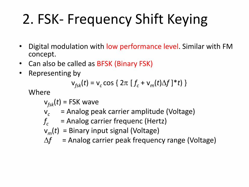
2. FSK- Frequency Shift Keying
• Digital modulation with low performance level. Similar with FM concept.
• Can also be called as BFSK (Binary FSK) • Representing by
vfsk(t) = vc cos { 2 [ fc + vm(t)f ]*t) } Where vfsk(t) = FSK wave vc = Analog peak carrier amplitude (Voltage)
fc = Analog carrier frequenc (Hertz)
vm(t) = Binary input signal (Voltage) f = Analog carrier peak frequency range (Voltage)
Teknik Pemodulasi Digit
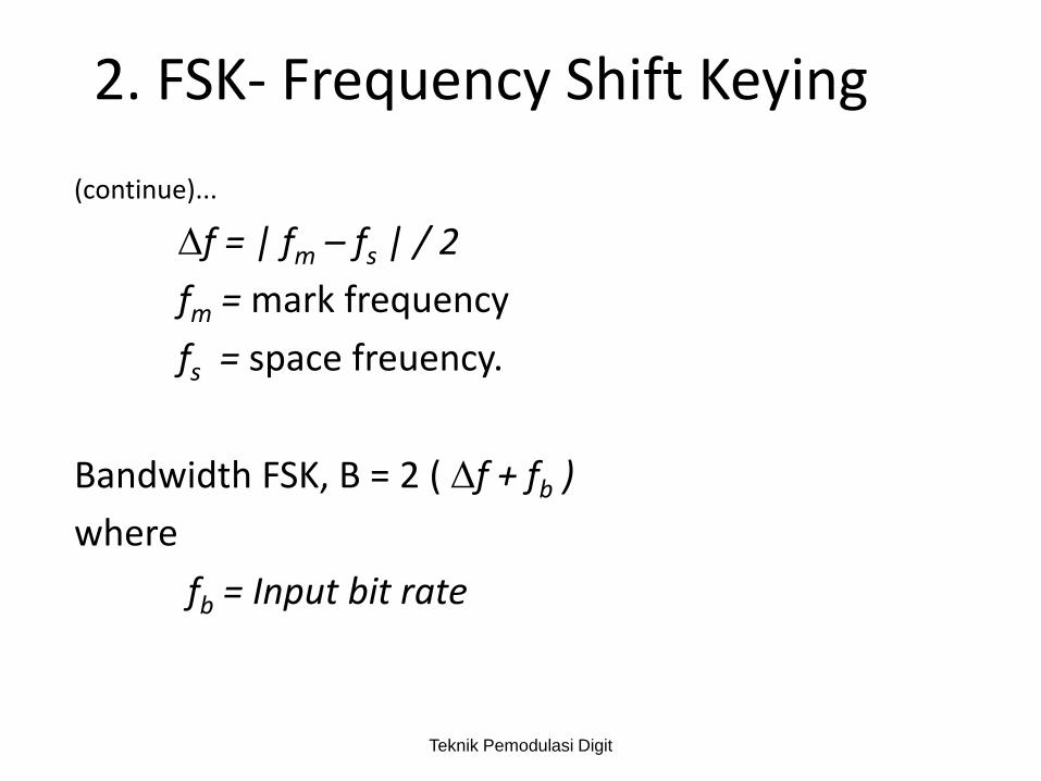
2. FSK- Frequency Shift Keying
(continue)...
f = | fm – fs | / 2
fm = mark frequency
fs = space freuency.
Bandwidth FSK, B = 2 ( f + fb )
where
fb = Input bit rate

2. FSK- Frequency Shift Keying
FSK wave represent in time domain, where
fc= 4 kHz
fs fm fs fs fs fs fs fm fm fm

FSK- Frequency Shift Keying
Binary Input Output
Frequency
‘0’ Space ( fs )
‘1’ Mark ( fm )
Truth table for FSK

Gaussian Minimum-Shift Keying A special case of FSK called Gaussian Minimum-Shift Keying (GMSK) is used in the GSM cellular radio and PCS systems to be described later. In a minimum shift system, the mark and space frequencies are separated by half the bit rate, that is,
0.5m s bf f f Here,
Frequency transmitted for mark (binary 1)
Frequency transmitted for space (binary 0)
Bit rate
mf
sf
bf

If we use the conventional FM terminology (refer to FM slides), we see that GMSK has a deviation each way from the center (carrier) frequency of,
0.25 bf Which corresponds to modulation index of
f
m
mf
0.25 b
b
f
f
0.25

Example: The GSM cellular radio system uses GMSK in a 100 kHz
channel, with a channel data rate of 170 kb/s. Calculate:
(a) The frequency shift between mark and space
(b) The transmitted frequencies if the carrier (center) frequency is
exactly 880 MHz
(c) The bandwidth efficiency of the scheme in b/s/Hz.
Answer:
(a) The frequency shift is
0.5 0.5 170 85m s bf f f kHz kHz

(b) The shift each way from the carrier frequency is half that found in (a), so the maximum frequency is
And the minimum frequency is
(c) The GSM system has a bandwidth efficiency of
170/100=1.7 b/s/Hz, comfortably under the theoretical maximum of 2 b/s/Hz for a two-level code.
max 0.25 880 0.25 170 922.5c bf f f MHz kHz MHz
min 0.25 880 0.25 170 837.5c bf f f MHz kHz MHz
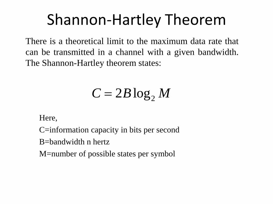
Shannon-Hartley Theorem There is a theoretical limit to the maximum data rate that
can be transmitted in a channel with a given bandwidth.
The Shannon-Hartley theorem states:
22 logC B M
Here,
C=information capacity in bits per second
B=bandwidth n hertz
M=number of possible states per symbol

Shannon Limit The information capacity of a channel cannot be increased
without limit by increasing the number of states because
noise makes it difficult to distinguish between signal
states. The ultimate limit is called the Shannon limit:
2log (1 / )C B S N
Here,
C=information capacity in bits per second
B=bandwidth n hertz
S/N=signal to noise ratio (as a power ratio, not in decibels)

Example: A radio channel has a bandwidth of 12 kHz and a signal to
noise ratio of 20 dB. What is the maximum data rate that can be
transmitted:
(a) Using any system?
(b) Using a code with four possible states? M=4

Example: A radio channel has a bandwidth of 12 kHz and a signal to
noise ratio of 20 dB. What is the maximum data rate that can be
transmitted:
(a) Using any system?
(b) Using a code with four possible states? M=4
Answer:
(a) We need the signal to noise ratio as a power ratio.
We can convert the given decibel value as follows:
1 20
log10
S
N
100
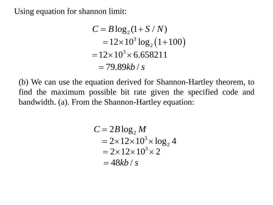
Using equation for shannon limit:
2log (1 / )C B S N
3
212 10 log 1 100 312 10 6.658211
79.89 /kb s
(b) We can use the equation derived for Shannon-Hartley theorem, to
find the maximum possible bit rate given the specified code and
bandwidth. (a). From the Shannon-Hartley equation:
22 logC B M3
22 12 10 log 4 32 12 10 2
48 /kb s

Since this is less than the maximum possible for this channel, it should be possible to transmit over this channel, with a four-level scheme, at 48 kb/s. A more elaborate modulation scheme would be required to attain the maximum data rate of 79.89 kb/s for the channel.
We will then have to compare this answer with that of part

Example: A typical dial-up telephone connection has a bandwidth of 2 kHz
and a signal to noise ratio of 20 dB. Calculate the Shannon limit.

Example: A typical dial-up telephone connection has a bandwidth of 2 kHz
and a signal to noise ratio of 20 dB. Calculate the Shannon limit.
Answer:
We need the signal to noise ratio as a power ratio. We
can convert the given decibel value as follows:
1 20
log10
S
N
100
2log (1 / )C B S N
3
22 10 log 101
13.316 /kb s
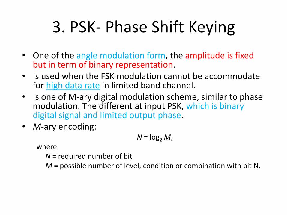
3. PSK- Phase Shift Keying
• One of the angle modulation form, the amplitude is fixed but in term of binary representation.
• Is used when the FSK modulation cannot be accommodate for high data rate in limited band channel.
• Is one of M-ary digital modulation scheme, similar to phase modulation. The different at input PSK, which is binary digital signal and limited output phase.
• M-ary encoding: N = log2 M, where N = required number of bit M = possible number of level, condition or combination with bit N.

3. PSK- Phase Shift Keying
• BPSK is the easiest form of PSK, where N = 1 and M = 2.
• Therefore, BPSK only has 2 phase at carrier, which are logic ‘1’ phase and logic ‘0’ phase.
• Can be called as Phase Reversal Keying (PRK) and Biphase Modulation
• Advantages: Improvement of the BER performance
• Disadvantages: Spectral is not efficient due to rapid phase with the presence of bit 1
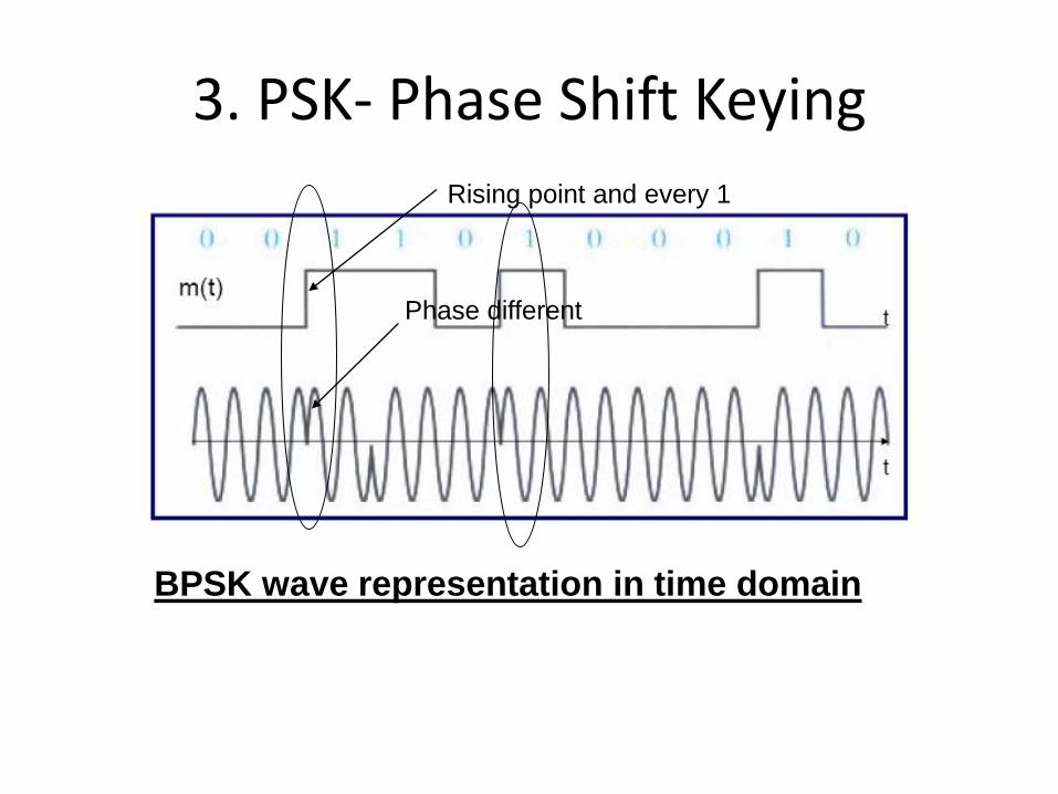
3. PSK- Phase Shift Keying
BPSK wave representation in time domain
Rising point and every 1
Phase different
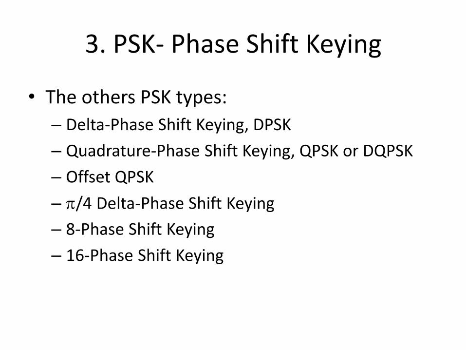
3. PSK- Phase Shift Keying
• The others PSK types:
– Delta-Phase Shift Keying, DPSK
– Quadrature-Phase Shift Keying, QPSK or DQPSK
– Offset QPSK
– /4 Delta-Phase Shift Keying
– 8-Phase Shift Keying
– 16-Phase Shift Keying
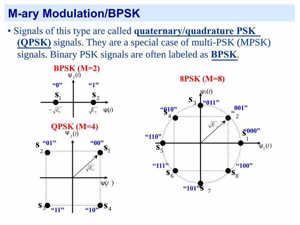
M-ary Modulation/BPSK • Signals of this type are called quaternary/quadrature PSK
(QPSK) signals. They are a special case of multi-PSK (MPSK)
signals. Binary PSK signals are often labeled as BPSK.
BPSK (M=2)
ψ (t)
2
“0” “1”
s s
8PSK (M=8)
ψ2(t)
1
− E E
2
ψ(t) “010”
s
3 “011” 001”
b b 1
QPSK (M=4)
s
4
E
s
“
2
“000”
ψ 2
(t
)
s
“110”
1
“01”
“00”
ψ
(t
)
s
s
s 1
2
E
1 5
“111” “100”
s
s
ψ(t
1
s
s )
s
6 8
“101”s
7
3
“11”
“10”
4

4. QAM- Quadrature Amplitude Modulation
• Similar to PSK, additional on carrier amplitude.
• The technique is used to obtain high data rate in a band limited channel.
• The elements position in constellation diagram is optimized so that:
– The distance between element is maximized (dynamic range increased)
– Low error possibility
4. QAM- Quadrature Amplitude Modulation
• Advantage: High data rate and more bandwidth efficient as compared to FSK or QPSK
• Disadvantage: Easier to be influenced by noise and the amplitude is always changing.
• Types of QAM: – 4-QAM
– 8-QAM
– 16-QAM
– ....

Quadrature Amplitude Modulation (QAM) • More general types of multi-symbol signaling schemes may be
generated by letting ai and bi take on multiple values themselves.
• The resultant signals are QAM signals. Therefore QAM is a
combined multi-phase/multi-amplitude signaling scheme.
16-QAM
“0000”
s
ψ
“0001” s
2
(t)
“0011” s
“0010”
s
1 2
3
3 4
“1000”
s
“1001” “1011” “1010”
s s s 5 6
1
-3 -1
s s
7 8
1 3
ψ s s
1
(t)
9
10
-1
11
12
“1100” “1101”
s s
“1111” “1110”
s s
13 14
-3
15 16 “0100”
“0101”
“0111”
“0110”
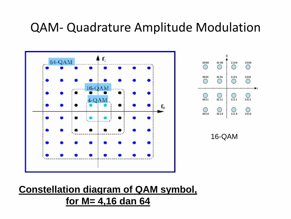
QAM- Quadrature Amplitude Modulation
Constellation diagram of QAM symbol,
for M= 4,16 dan 64
16-QAM

QPSK: Without Pulse Shaping
Data
0
0
1
1
Data
0
1
0
1
Data
00
01
180o
10
11
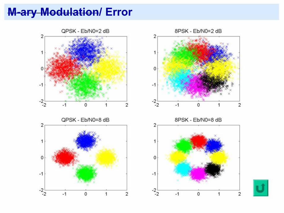
M-ary Modulation/ Error
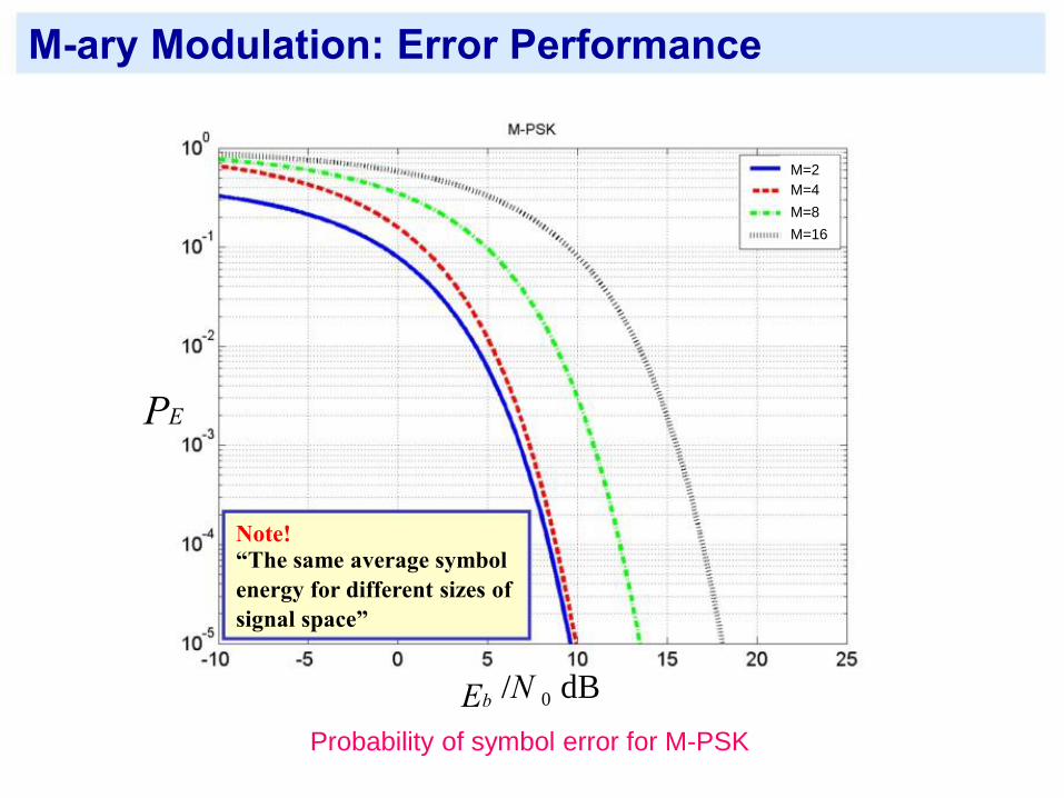
M-ary Modulation: Error Performance
M=2
M=4
M=8
M=16
PE
Note!
“The same average symbol
energy for different sizes of
signal space”
Eb
/N
0
dB
Probability of symbol error for M-PSK
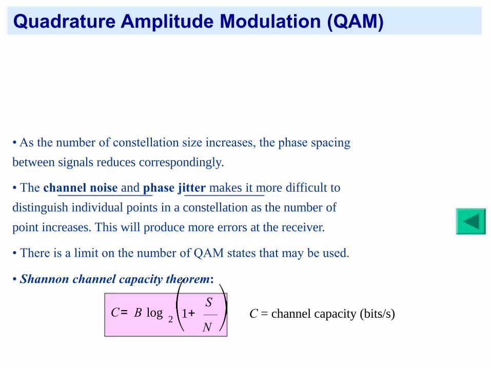
Quadrature Amplitude Modulation (QAM)
• As the number of constellation size increases, the phase spacing
between signals reduces correspondingly.
• The channel noise and phase jitter makes it more difficult to
distinguish individual points in a constellation as the number of
point increases. This will produce more errors at the receiver.
• There is a limit on the number of QAM states that may be used.
• Shannon channel capacity theorem:
⎛
S
⎞
C
=
B
log
2
1+ ⎝ N
⎠
C = channel capacity (bits/s)

5. CPM- Continuous Phase Modulation
• The phase of carrier signal is continously modulated.
• The signal power is mostly homogeneous; advantages of CPM as compared to other digital modulation schemes.
• Memory phase; phase for every signal is determined by total of cumulative phase of the prior signal.
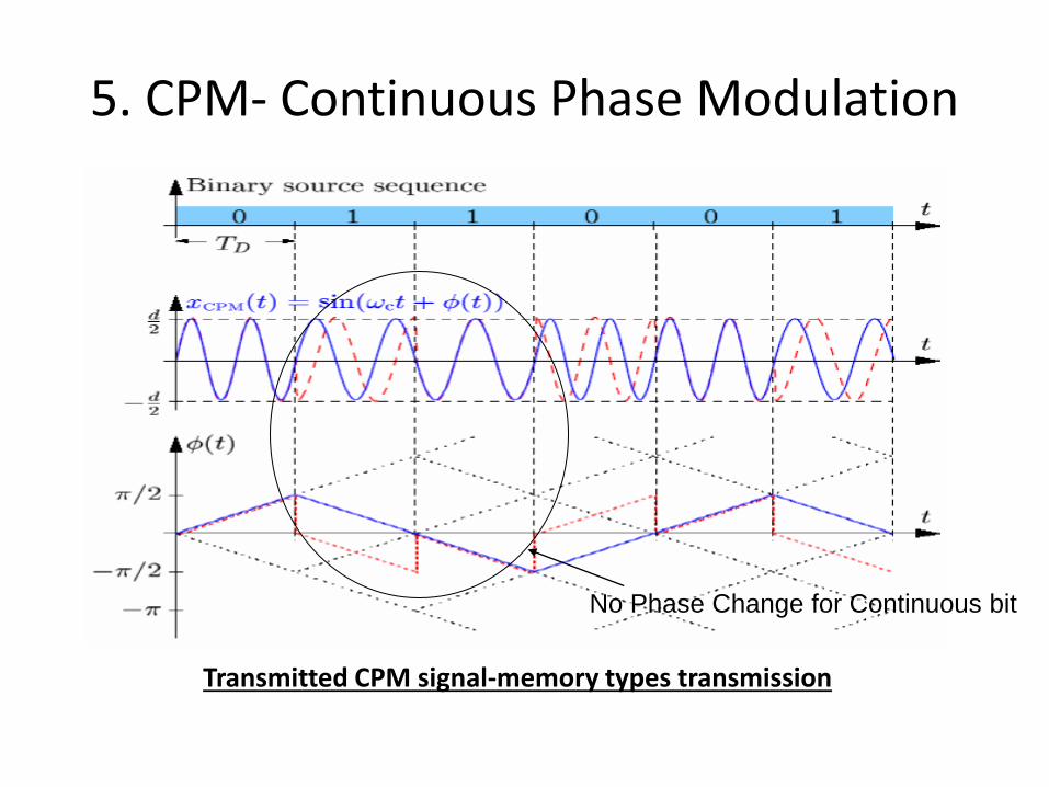
5. CPM- Continuous Phase Modulation
Transmitted CPM signal-memory types transmission
No Phase Change for Continuous bit

Minimum-Shift-Keying (MSK) MSK: wider mainlobe, but
better energy compaction,
hence more bandwidth
efficient
QPSK: energy spreading out,
hence not bandwidth efficient
MSK: lower sidelobes
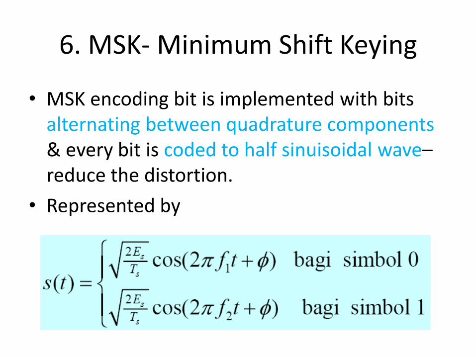
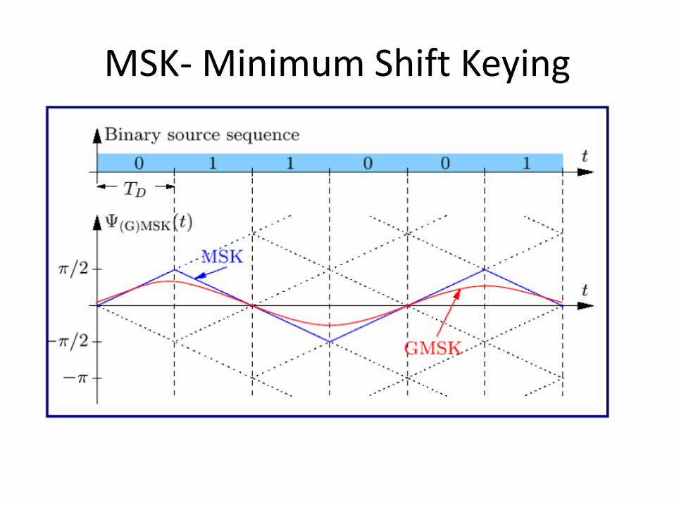
6. MSK- Minimum Shift Keying
• MSK encoding bit is implemented with bits alternating between quadrature components & every bit is coded to half sinuisoidal wave– reduce the distortion.
• Represented by
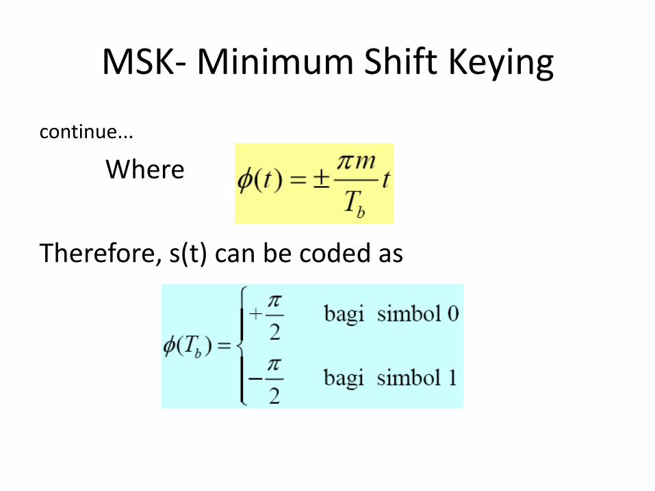
MSK- Minimum Shift Keying
continue...
Where
Therefore, s(t) can be coded as
MSK- Minimum Shift Keying
148
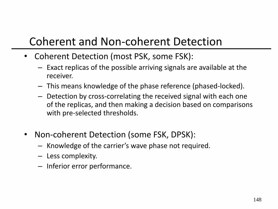
Coherent and Non-coherent Detection • Coherent Detection (most PSK, some FSK):
– Exact replicas of the possible arriving signals are available at the receiver.
– This means knowledge of the phase reference (phased-locked).
– Detection by cross-correlating the received signal with each one of the replicas, and then making a decision based on comparisons with pre-selected thresholds.
• Non-coherent Detection (some FSK, DPSK): – Knowledge of the carrier’s wave phase not required.
– Less complexity.
– Inferior error performance.

149
Design Trade-offs • Primary resources:
– Transmitted Power.
– Channel Bandwidth.
• Design goals:
– Maximum data rate.
– Minimum probability of symbol error.
– Minimum transmitted power.
– Minimum channel bandiwdth.
– Maximum resistance to interfering signals.
– Minimum circuit complexity.
150
Book References :
Blake, R. 2002. Electronic Communication Systems, 2/e. Australia: Cengage Delmar Learning. ISBN: 0766826848.
Couch, L. W. 2007. Digital and Analog Communication Systems, 7/e. New Jersey: Prentice-Hall. ISBN: 0-13-203794-7.
Fitz, M. P. 2007. Fundamentals of Communications, 5/e. McGraw Hill
Lathi, B.P. 2003. Modern Digital and Analog Communications Systems, 3/e. Oxford University Press, ISBN 0-19-511009-9.
Zahedi, E. 2002. Digital Data Communication, Pearson Education, Prentice Hall.