MODIFICATIONS TO THE DCF STOCK V~LUATION MODEL

Eugene F. Brigham and T. Craig Tapley

Public Utility Research Center

University of Florida

November 1984

PURC Working Paper Series

November 2, 1984

Modifications to the OCF Stock Valuation Model

In 1938, J. B~ Williams [5] developed the concept that a stock's

value is determined as the present value of its expected future dividend

stream. Following up on Williams' work, Gordon and Shapiro [2] solved

the discounted cash flow (DCF) stock valuation model for k, the required

rate of return, and then discussed the use of this DCF k as the firm's

cost of equity. Gordon and others went on to use the DCF model for many

purposes, and versions were developed to deal with situations where the

expected future growth rate is variable as well as constant. However,

in almost all of the publications we ha~e seen, including the;"leading

textbooks, applications of the DCF model are based on two incorrect

assumptions: (1) that dividends are paid annually, whereas they are

actually paid quarterly, and (2) that the analysis takes place on a

dividend paYment date, so that the next dividend will be received

exactly one year after the current date. 1

lThe dividend payment date problem involves both the ex-dividend dateand the actual payment date. In the typical DCF analysis, peoplegenerally assume implicitly (1) that we are at the ex-dividend date and(2) that the payment date and the ex-dividend date are the same. Thisis clearly not true. For example, at the bottom of the Value Linereport on BellSouth dated July 27, 1984, it is noted that the stock willgo ex dividend on September 24, with payment to be made on November 1.Thus, an investor who buys the stock on September 23 will receive theNovember 1 dividend, so he or she will have to wait only 38 days before

I receiving a payment. On the other hand, an investor who buys the stockon September 24 will not receive the November dividend, and he or shewill have to wait more than one full quarter before receiving the firstdividend payment (37 + 90 = 127 days). The price of a share of stocknormally falls by the tax-adjusted present value of the next dividend tobe paid when the stock goes ex-dividend. Other things held constant,stock prices rise between ex-dividend dates, decline on the ex-dividenddate, and continue to cycle in this manner over time, but with an upwarddrift to reflect long-term growth.

-2-

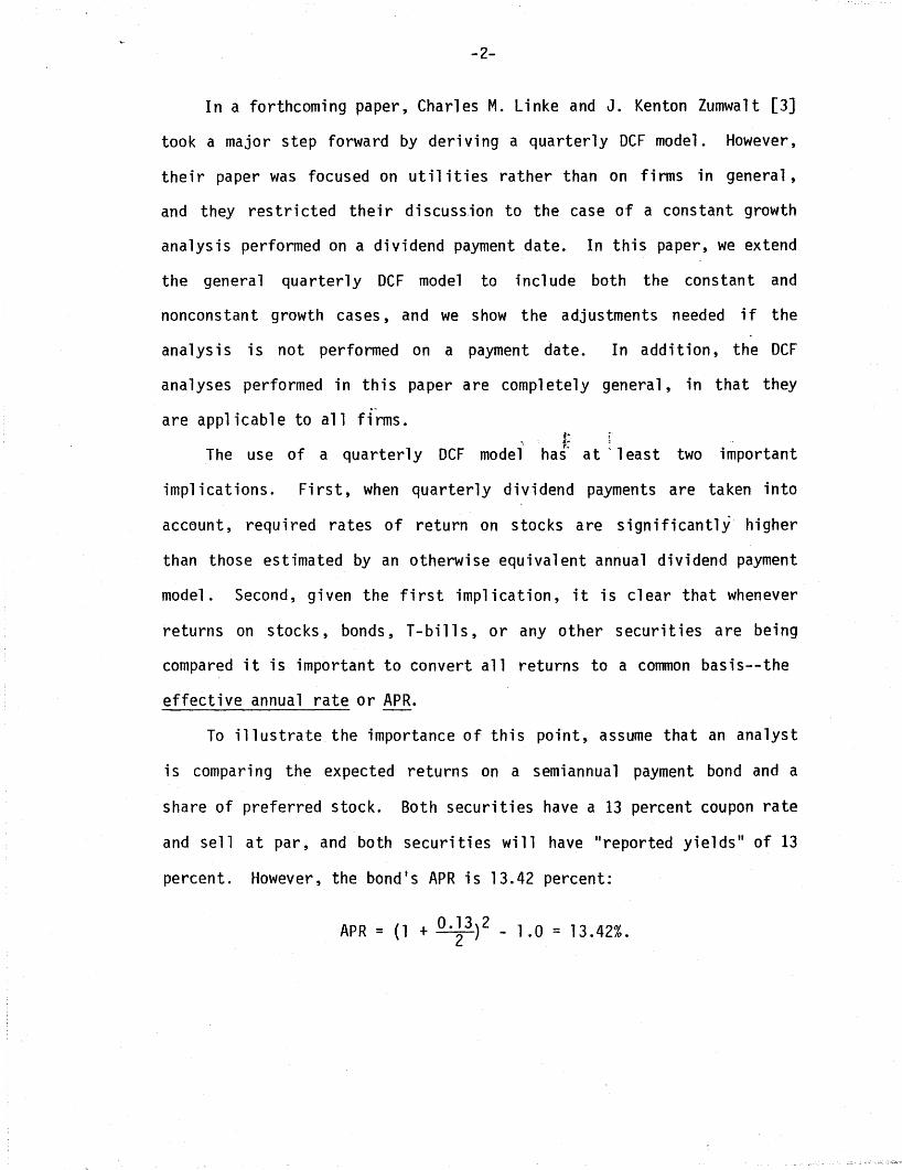
In a forthcoming paper, Charles M. Linke and J. Kenton Zumwalt [3]

took a major step forward by deriving a quarterly DCF model. However,

their paper was focused on util ities rather than on firms in general,

and they res tri cted thei r di scuss.ion to the case of a cons tant growth

analysis performed on a dividend payment date. In this paper, we extend

the general quarterly DCF model to include both the constant and

nonconstant growth cases, and we show the adjustments needed if the

analysis is not performed on a payment date. In addition, the DCF

analyses performed in this paper are completely general, in that they

are applicable to all firms.

The use of a quarterly DCF model;~

$~

has' at·· 1east two important

impl ications. First, when quarterly dividend payments are taken into

account, required rates of return on stocks are significantly higher

than those estimated by an otherwise equivalent annual dividend payment

model. Second, given the first implication, it is clear that whenever

returns on stoc ks, bonds, T- bi 11 s, 0 r any other securi ties are bei ng

compared it is important to convert all returns to a common basis--the

effective annual rate or APR.

To illustrate the importance of this point, assume that an analyst

is comparing the expected returns on a semiannual payment bond and a

share of preferred stock. Both securities have a 13 percent coupon rate

and sell at par, and both securities will have "reported yields" of 13

percent. However, the bond's APR is 13.42 percent:

APR = (1 + 0.13)2 - 1.0 = 13.42%.

-3-

The preferred stock ($100 par) pays interest of $3.25 each quarter.

Using an annual OCF model, the simple annual yield on the preferred

would also be 13 percent:

Annual yield = ($3. 25 ) (4) =$100 13.00%.

However, the. APR yield on the preferred will be 13.65 percent:

APR = (1 + 0413)4 - 1.0 = 13.65%.

If the analyst compared these securities using simple annual rates, hei-c·

or she would conclude that they both yield 13 percent. However, on an

APR basis, the effective return on the preferred stock exceeds that on

the bond by 13.65% - 13.42% = 0.23%, or 23 basis points. Th'us, when

comparing the yields on different types of securities, it is important

to put all returns on an APR basis to avoid an app1es-to-oranges

comparison.

The quarterly OCF model which we develop in this paper provides a

method for calculating the APR on a share of stock. Still, the primary

benefi t of ou r model is thatit provi des a general i zed OCF framework,

which properly accounts for dividend payment patterns and for the actual

timing of dividend receipts.

The paper is divided into three sections. First, we discuss OCF

models in general. Next, we develop constant and nonconstant growth OCF

models, and we demonstrate how they can be used. Finally, we provide a

brief summary and restatement of our conclusions.

..

-4-

OCF Models in General

For common stock, the general OCF model may be defined as follows:

o 0 0Value = P = 1 + 2 + •.. + 00 (1)

o (1 + k)l (1 + k)2 (1 + k)oo'

where Po is the current price of the stock, 0t is the expected periodic

dividend, and k is the required rate of return. Under a certain set of

assumptions, Equation 1 reduces to Equation 2: 1

(2)

which may be solved for k to produce Equation 3, the constant

growth/annual payment OCF equation:

01k = P + g,o

(3)

where 01 is the dividend expected at the end of the next period and g is

the constant expected growth rate for earnings, dividends, and the stock

price.

Equations 2 and 3 are correct if and only if (1) the price, PO' is

determined on a dividend payment date, (2) the next dividend, D1, will

be received exactly one period hence, (3) each dividend will increase at

the rate g, and (4) g is constant, which implies that both the return on

lFor a derivation of this model, see E. F. Brigham, [1, Chapter 5].

-5-

equity (ROE) and the payout ratio are expected to remain constant. The

top panel of Figure 1 shows the dividend payment pattern assumed in the

constant growth/annual payment model inherent in Equations 2 and 3.

In the real world, we know that dividends are normally paid

quarterly and increased once a year as shown in the lower panel of

Figure 1. Further, the analysis could take place at times other than a

dividend payment date, so the length of time until the next dividend is

received, and also until the dividend is increased, could vary from case

to case. Finally, the dividend growth rate is not always expected to be

constant. For example,'a finm in the early stages of its life cycle, or;-- ;"'.

a firm in an industry that is experienciny rapid technological thanges,

may have an expected growth rate in the short-run that is either higher

or lower than the average growth rate expected over the long run. For

such a firm, a multi-stage (or nonconstant) DCF model of this form

should be used:

Dl + D2 + ... + _D_n _ + (Dn(l + g)\f.. 1 )n(1 + k)l (1 + k)2 (1 + k)n \ k - g }\1 + k

(4)

Dividends during Periods 1 to n could be either constant (no growth),

growing at a constant rate different from the terminal growth rate,

decl ining, or growing at different rates from year to year. However,

the model does assume that all dividends received after Period n will

I grow at a constant, long-run growth rate, g, so the last term in Equa­

tion 4 is the present value of all dividends expected beyond Year n as

determined by the constant growth model. To use the nonconstant model,

one must obtain specific dividend forecasts for Years 1 to n, as well as

Dividends($)

1.00

-6-

Figure 1

Annua 1 Payments

o

Dividends($)

1 2 3 4 5 Periods

1.00

Quarterly Payments

___--J • • • •

3.... 1'4

. 2 3I I I I I I ,

4 5 Peri ods

-7-

an estimate of the long-run, steady-state growth rate, g, and then solve

for k, the DCF cost of equity.l

Equation 4 is conceptually superior to Equation 2 in situations

where there is reason to believe that investors do not expect a constant

growth rate, but it is still based on two incorrect assumptions, namely,

that dividends are paid annually and that the analysis always occurs on

a dividend payment date. These incorrect assumptions can lead to

incorrect estimates of the cost of equity.

In terms of practical applications, the annual model is somewhat

easier to derive and to· use than the quarterly model. Further, even;~ r

. s· ;

though the quarterly model is theoretical"ly correct, it cannot be easily

eva1uated except by the use of a computer model. However, although

thes~ computer model s used to be hard to develop, with a personal

computer and an electronic spreadsheet such as Lotus 1-2-3, it is now

relatively easy to set up and solve either the constant or the

nonconstant quarterly DCF model, and to adjust for pricing at dates

other than the dividend payment date. Thus, the procedures we discuss

below are not at all difficult to implement in actual practice.

Constant Growth Quarterly DCF Models

Equation 1 above assumes that the next dividend will be paid

exactly one period from the analysis date. If the analysis is done

between payment dates, with f l being the fraction of a period before the

lWe illustrate Equation 4 later in the paper.

-8-

nex t payment wi 11 be made, then we can trans form Equa t ion 1 into

Equation 5:

D1 D2f + ---~f~ + ... + ----:f-·(1 + k) 1 (1 + k) 2 (1 + k) 00

(5)

This equation is completely general, so it can be applied to the case of

a company which pays quarterly dividends and increases them once a year.

For example, suppose a company's stock sells for $29.25; it is expected

to pay an annual dividend of $2.60, or $0.65 per quarter over the coming

year; dividends are growing at 7 percent;:per year; and the com~any has

just paid the last of the quarterly dividends at the old rate. The

valuation equation then becomes:

$29.25 = 0.65 + 0.65 + 0.65 + 0.65 + 0.65(1.07) + ....(1 + k)·25 (1 + k)·50 (1 + k)·75 (1 + k)l (1 + k)1.25

The first exponent, f 1, represents the fraction of the year before a

purchaser of the stock will receive his or her first dividend, and in

this example we assume that the first dividend will be received at the

end of one quarter. Each subsequent exponent is increased by 0.25, that

is, f t +1 = f t + 0.25.

From a practical viewpoint, there are two problems with Equation 5.

First, it is obviously not feasible to extend it on out to infinity and

then to solve for k. Second, we might want to determine a company's

cost of capital on some date other than the dividend payment date.

Fortunately, both problems can be solved by use of the following model,

which is derived in Appendix A:

-9-

Here

0, through 04 are the next four quarterly dividends expe~ted to be

received over the coming year. If the analysis is done during

the first quarter of the firm's "dividend year" and before the

ex-dividend date, then 01 through· 04 will be equal. However,

if the analysis is done during the second, third, or fourth

quarters, then two different quarterly dividend amounts will;,,,. r"

.: &~ ;

be reflected in the numerator bf Equation 6.

f, is the fraction of a year before the first dividend is received,

so , - f, is the fraction of the year between the time the

first dividend is received and the end of the year, the end of

the year being 12 months after the analysis date. When we

consider ex-dividend dates, f1 wi" normally be in the range

of 0.10 to 0.35, so , - f, wi1' normally range from 0.90 to

0.65.

f2' f3' and f4 are the fract ions of the year before the second,

third, and fourth dividends are received.'

Several points should be noted regarding Equation 6:

1To be exactly correct, this model should use a 365-day year, and theactual number of days between each payment date should be calculated.However, it is much easier to apply the model using a 360-day year and90-day quarters. Further, our studies indicate that this simplificationgenerally results in an error of less than one basis point.

-10-

1. The derivation of Equation 6 from Equation 5, as set forth inAppendix A, is similar to the derivation of Equations 2 and 3 from1, but there are many more terms in the quarterly model, and henceboth the derivation and the final model (Equation 6) are morecomplex than with the annual model.

2. The annual model assumes that one dividend is paid at the end ofthe year, so 0 in the annua1 model is the sum of the fourdividends expecled over the next four quarters. However, thesefourdi vi dends do not have to have the same val ue. For -examp1 e, acompany might be currently paying an annual dividend of $2.60, or$0.65 per quarter, with two of the 65 cent dividends having alreadybeen paid. If its expected growth rate is 7 percent, then itsannual dividend rate should go to $2.60(1.07) = $2.78, which thenimp1 ies that its quarterly dividend shou1 d increase to approxi­mately $0.70 two quartrrs hence. Therefore, 01 = $0.65 + $0.65 +$0.70 + $0.70 = $2.70 .

.-3. The quarterly model recognizes that dividends are received

quarterly, that they can be reinv~sted in the market tQ~ earn areturn of k percent, and therefore that the compounded value of thedividends at the end of the year will be greater than the simplesum of the quarterly dividends. Thus, the dividend yield in thequarterly model exceeds that found with the annual model as it is

- generally applied. For example, suppose a stock sells for $29.25,is expected to pay $2.60 over the next four quarters ($0.65 perquarter), and has its first payment due in 90 days. If the growthra te is cons tant at 7 percent, then the annual model produces acost of 15.89%:

°1 _ $ 2.60k = Po + g - $29.25 + 7%

= 0.0889 + 0.070 = 15.89%.

Thus, according to the traditional OCF model, an investor whobought the s toc k wou 1d expect to earn a return of 15.89 percen t.However, with the quarterly model, we insert the known values intoEquation 6,

= $0.65(l+k)0.75+ $0.65(l+k)0.50+ $0.65(1+k)0.25+ $0.65(l+k)0k $29.25 + 0.07,

l Some security analysts use as 01

the latest quarterly dividend times 4.This understates 01 except just after a dividend increase has beenannounced but before the s toc k goes ex for the fi rs t of the newdividends. Other analysts find 0 as the latest quarterly dividendtimes 4, multiplied by (1 + g). T~is procedure overstates the expecteddividend except just after the stock has gone ex dividend for the lastof the old, lower dividends.

-11-

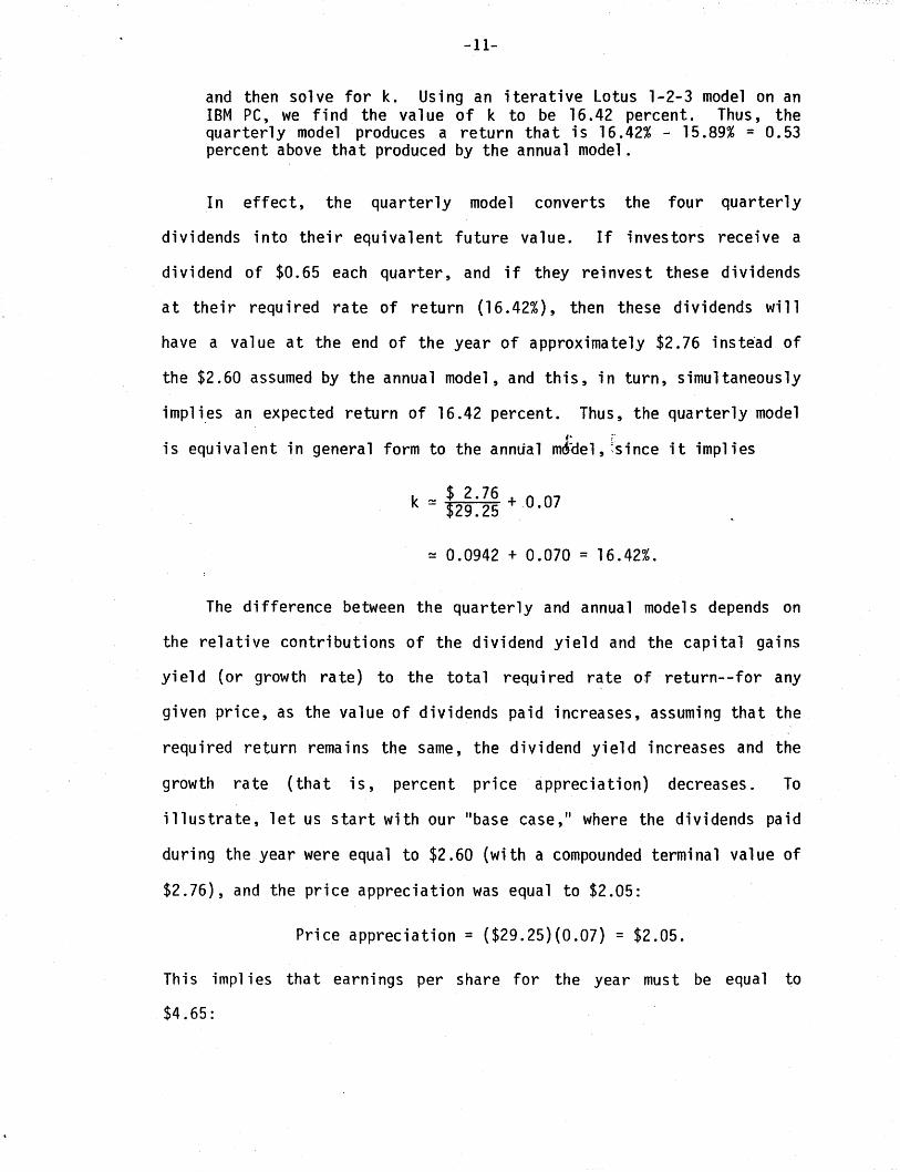
and then solve for k. Using an iterative Lotus 1-2-3 model on anIBM PC, we find the value of k to be 16.42 percent. Thus, thequarterly model produces a return that is 16.42% - 15.89% = 0.53percent above that produced by the annual model.

In effect, the quarterly model converts the four quarterly

dividends into their equivalent future value. If investors receive a

dividend of $0.65 each quarter, and if they reinvest these dividends

at their required rate of return (16.42%), then these dividends will

have a value at the end of the year of approximately $2.76 insteOad of

the $2.60 assumed by the annual model, and this, in turn, simultaneously

imp1ies an expected return of 16.42 percent. Thus, the qua rter1y modeli-"" ;"

is equivalent in general form to the annlial mctdel, ~since it implies

$ 2.76k ~ $29.25 +.0.07

~ 0.0942 + 0.070 = 16.42%.

The difference between the quarterly and annual models depends on

the relative contributions of the dividend yield and the capital gains

yield (or growth rate) to the total required rate of return--for any

given price, as the value of dividends paid increases, assuming that the

required return remains the same, the dividend yield increases and the

growth rate (that is, percent price appreciation) decreases. To

illustrate, let us start with our "base case," where the dividends paid

during the year were equal to $2.60 (with a compounded terminal value of

$2.76), and the price appreciation was equal to $2.05:

Price appreciation = ($29.25)(0.07) = $2.05.

This impl ies that earnings per share for the year must be equal to

$4.65:

-12-

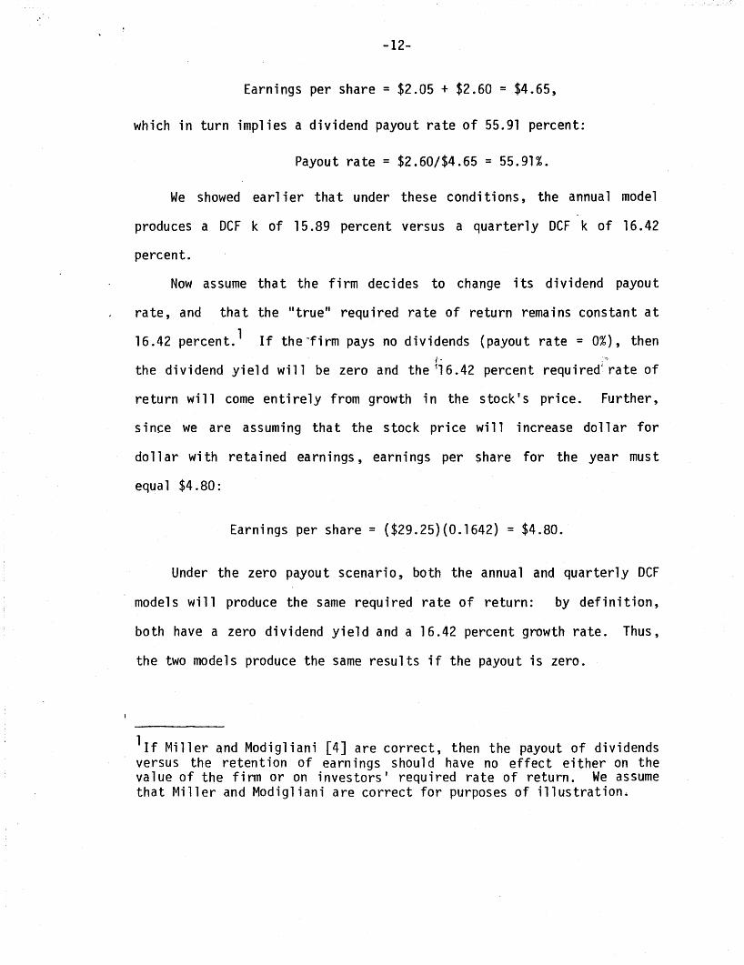
Earnings per share = $2.05 + $2.60 = $4.65,

which in turn implies a dividend payout rate of 55.91 percent:

Payout rate = $2.60/$4.65 = 55.91%.

We showed ea rl ier tha t under these condi ti ons, the annua1 model

produces a OCF k of 15.89 percent versus a quarterly OCF k of 16.42

percent.

Now assume that the firm decides to change its dividend payout

rate, and that the "true" required rate of return remains constant at

16.42 percent. 1 If the "firm pays no dividends (payout rate = 0%), thenj- .

the dividend yield will be zero and the ~16.42 percent required~rate of

return will come entirely from growth in the stock's price. Further,

since we are assuming that the stock price will increase dollar for

dollar with retained earnings, earnings per share for the year must

equal $4.80:

Earnings per share = ($29.25)(0.1642) = $4.80.

Under the zero payout scenario, both the annual and quarterly OCF

models will produce the same required rate of return: by definition,

both have a zero dividend yield and a 16.42 percent growth rate. Thus,

the two models produce the same results if the payout is zero.

lIf Miller and Modigliani [4] are correct, then the payout of dividendsversus the retention of earnings should have no effect either on thevalue of the firm or on investors' required rate of return. We assumethat Miller and Modigliani are correct for purposes of illustration.

-13-

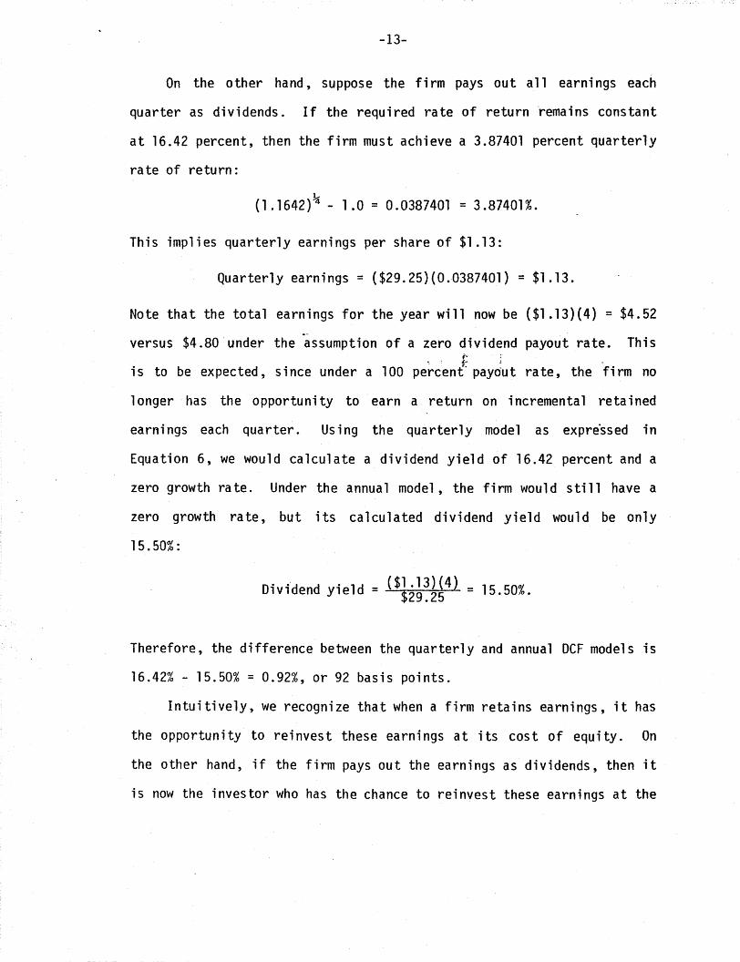
On the other hand, suppose the fi rm pays out all earni ngs each

quarter as dividends. If the required rate of return remains constant

at 16.42 percent, then the firm must achieve a 3.87401 percent quarterly

ra te of return:

1

(1 .1642)~ - 1.0 = 0.0387401 = 3.87401%.

This implies quarterly earnings per share of $1.13:

Quarterly earnings = ($29.25)(O.D38740l) = $1.13.

Note that the total earnings for the year will now be ($1.13)(4) = $4.52

versus $4.80·under the assumption of a zero dividend payout rate. This,., ;

• s- :

is to be expected, since under a 100 percent' payout rate, the firm no

longer· has the opportuni ty to earn a return on incremental reta i ned

earnings each quarter. Using the quarterly model as expressed in

Equation 6, we would calculate a dividend yield of 16.42 percent and a

zero growth rate. Under the annual model, the firm would still have a

zero growth rate, but its calculated dividend yield would be only

15.50% :

Dividend yield = ~~-=-=:---Z- = 15.50%.

Therefore, the difference between the quarterly and annual DCF models is

16.42% - 15.50% = 0.92%, or 92 basis points.

Intuitively, we recognize that when a firm retains earnings, it has

the opportunity to reinvest these earnings at its cost of equity. On

the other hand, if the firm pays out the earnings as dividends, then it

is now the investor who has the chance to reinvest these earnings at the

-14-

cost of equity (required rate of return). The quarterly model takes

reinvestment into account, whereas the annual model does not.

Therefore, the higher the percentage of earnings paid out, the greater

the difference between the annual and quarterly models.

Table 1 shows the differences between the two models at varying

payout rates. The higher the payout, the larger the difference between

the two models, and the greater the annual model t s inherent downward

bias. This suggests that the quarterly' adjustment is particularly

important in industries where payout ratios tend to be high, such as the

utility industry.;~.

E­r.

Payment Date Adjustment

-Thus far we have assumed that the analysis occurs, ana Po is

observed, on a dividend payment date. If the analysis actually takes

place before or after a payment date, then this fact should be taken

into account. The quarterly model, as we use it, already reflects the

time until the next dividend, but the annual model requires the

following adjustment:

DPo = 1 (1 + k)tk - g ,

which impl i es

ok = __1 (1 + k)t + g.

Po

Here t is equal to (90 - days to receipt of next dividend)/360.

(7)

(8)

-15-

Table 1Differences between the Annual and

Quarterly DCF Models at Various Payout Rates

% Annual . Quarterly DifferencePayout DCF k DCF k in k

0 16.42% 16.42% 0.00%

25 16. 18 ~} 6.42 0.24

50 15.94 16.42 0.48

75 15.72 16.42 0.70

100 15.50 16.42 0.92

-16-

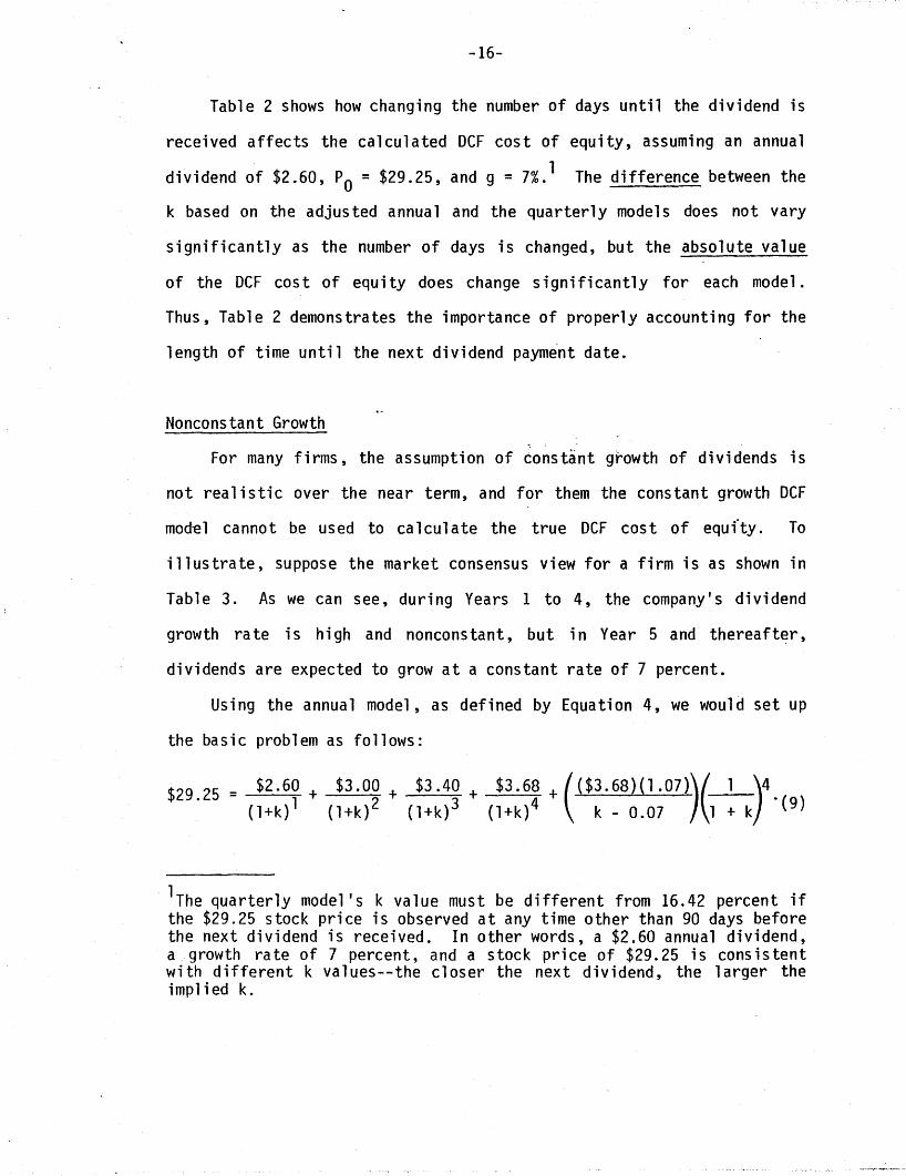
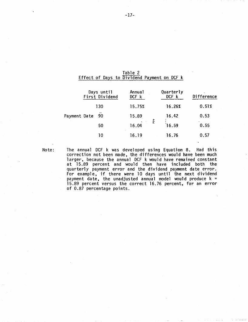
Table 2 shows how changing the number of days until the dividend is

received affects the calculated OCF cost of equity, assuming an annual

dividend of $2.60, Po = $29.25, and g = 7%.1 The difference between the

k based on the adjusted annual and the quarterly models does not vary

significantly as the number of days is changed, but the absolute value

of the OCF cost of equity does change significantly for each model.

Thus, Table 2 demonstrates the importance of properly accounting for the

length of time until the next dividend payment date.

Nonconstant Growth

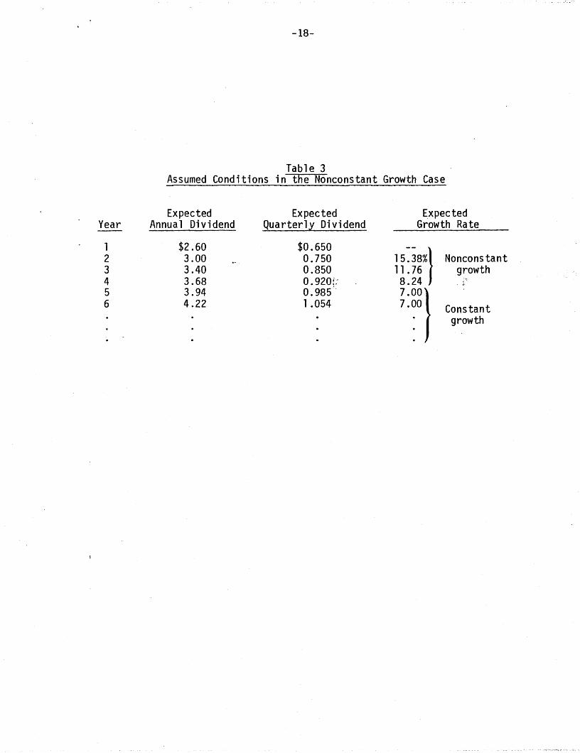
For many firms, the assumption of constant growth of dividends is

not realistic over the near term, and for them the constant growth OCF

mod-e1 cannot be used to calculate the true OCF cost of equfty. To

illustrate, suppose the market consensus view for a firm is as shown in

Table 3. As we can see, during Years 1 to 4, the company's dividend

growth rate is high and nonconstant, but in Year 5 and thereaft~r,

dividends are expected to grow at a constant rate of 7 percent.

Using the annual model, as defined by Equation 4, we would set up

the basic problem as follows:

$29.25 = $2.60 + $3.00 + $3.40 + $3.68 + (($3.68)(1.07)\( 1 )4{l+k)l {1+k)2 {1+k}3 {1+k}4 k - 0.07 I 1 + k '(9)

lThe quarterly model's k value must be different from 16.42 percent ifthe $29.25 stock price is observed at any time other than 90 days beforethe next dividend is received. In other words, a $2.60 annual dividend,a growth rate of 7 percent, and a stock price of $29.25 is consistentwith different k values--the closer the next dividend, the larger theimplied k.

-17-

Table 2Effect of Days to Dividend Payment on DCF k

Days until Annual QuarterlyFirst Dividend DCF k DCF k Difference

130 15.75% 16.26% 0.51%.-

Payment Date 90 15.89 16.42 0.53f", ~~

r.

50 16.04 ""16.59 0.55

10 16. 19 16.76 0.57

Note: The annual DCF k was developed using Equation 8. Had thiscorrection not been made, the differences would have been muchlarger, because the annual DCF k would have remained constantat 15.89 percent and would then have included both thequarterly payment error and the dividend payment date error.For examp1 e, if there were 10 days until the next dividendpayment date, the unadjusted annual model would produce k =15.89 percent versus the correct 16.76 percent, for an errorof 0.87 percentage points.

-18-

Table 3Assumed Conditions in the Nonconstant Growth Case

Expected Expected E.xpectedYear Annual Dividend Quarterly Dividend Growth Rate

1 $2.60 $0.65015~38%}2 3.00 0.750 Nonconstant

3 3.40 0.850 11 .76 growth4 3.68 0.920:: 8.245 3.94 0.985"

7ODD}6 4.22 1.054 7.00 Constant. growth.

-19-

This model can be solved for k using an iterative process; the solution

value is k = 17.09 percent. 1

Appendix A shows the derivation of a nonconstant quarterly growth

DCF model. However, the resulting equation is extremely complicated,

and the longer the peri od of noncons tant growth, the "mess i er" the

equation. Fortunately, we can analyze the nonconstant quarterly growth

case easily with an electronic spreadsheet and a personal computer.

These are the steps to be followed:

1. Specify the dividends to be received, on a quarterly basis, duringthe nonconstant growth period. Key these values into thespreadsheet model. ~

£1r.

2. Determine the fraction of the year before the first dividend isreceived. Each subsequent dividend will be received 0.25 periods1a ter.

3. Once the noncons tant growth years have ended, di vi dends wi 11 growevery fourth period at the rate g. (This situation is easy tomodel using a spreadsheet such as Lotus 1-2-3.)

4. The spreadsheet model thus defines this equation:

01f +

(1 + k) 1

O2f +

(1 + k) 2

DN..• + ----:::f-'

(1 + k) N

(10)

where f is the fraction of a year before the first dividend isreceiveJ, k is the cost of equity, and N is the number of quarters

1The cost of equity in this case, 17.09 percent, is higher than the15.89 percent found in the 7 percent constant growth case because, inthe new case, growth is much higher in the early years. The averagegrowth ra te is

g = k - Dl/PO = 0.1709 - $2.60/$29.25 = 17.09% - 8.89% = 8.20%,

where the 8.20 percent is a weighted average of the relatively highshort-run growth rates and the 7 percent long-run growth rate.

-20-

the model is to run. Theoretically, N should be set equal toinfinity, but as a practical matter, the present value of dividendsout beyond 200 years is virtually zero, so we can set N == 800quarters.

5. With all variables except k specified in the spreadsheet model, wehave the computer solve iteratively for k, setting the presentvalue of the future dividend stream equal to the current price.

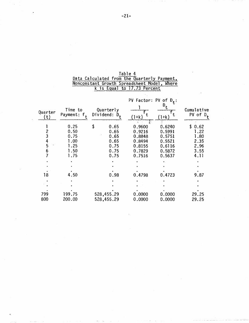
We can illustrate the nonconstant quarterly model with the data and

conditions set forth in Table 3 above. To simplify the explanation, we

assume that the analysis takes place on a dividend payment date, so

there is one fu 11 qua rter before the next dividend wi 11 be recei ved.

Under these assumptions'~ the DCF cos t of equi ty is found to be 17.73;.

percent, and the solution values for Equation 10,~ as generated by the

electronic spreadsheet, are shown in Table 4.

_The cost of equity, as calculated earlier by the annual . payment

model (Equation 9), 17.09 percent, may be compared to the 17.73 percent

found using the quarterly model. Thus, in this nonconstant growth

situation, the annual payment model involves an error of 17.73% - 17.09%

= 0.64%, or 64 basis points.

Summary and Conclusions

The primary purpose of this paper was to extend the traditional DCF

model to encompass the real istic case of quarterly dividends that are

increased annually. In addition, we demonstrate that the annual model,

if it is to be used, should be adjusted whenever the analysis occurs on

a date other than the dividend payment date. Both adjustments are

especially important for high payout firms such as the electric, gas,

and telephone companies.

-21-

Table 4Data Calculated from the Quarterly Payment,Nonconstant Growth Spreadsheet Model, Where

k is Equal to 17.73 Percent

PV Factor: PV of Dt :

Time to Quarterly 1 Dt Cumul ativeQuarter f f(t) Payment: f t Dividend: Dt (1 +k) t (1 +k) t PV of Dt,

'. ~~

r.

1 0.25 $ 0.65 0.9600 0.6240 $ 0.622 0.50 0.65 0.9216 0.5991 1.223 0.75- 0.65 0.8848 0.5751 1.804 1.00 0.65 0~8494 0.5521 2.355 1.25 0.75 0.8155 0.6116 2.966 1.50 0.75 0.7829 0.5872 3.557 1.75 0.75 0.7516 0.5637 4.11

18

.799800

.4.50

.199.75200.00

.0.98

.528,455.29528,455.29

.0.4798

.0.00000.0000

.0.4723

.0.00000.0000

.9.87

.29.2529.25

-22-

We are not sure what the implications of our study are for capital

budgeting. In capital budgeting, people often assume that cash flows

occur at the end of the year. If cash flows actually occur all during

the year, then perhaps this fact should be taken into account if a

quarterly adjusted OCF cost of equity is to be used in capital

budgeting. l

One could argue that, given the uncertainty inherent in the basic

data required for a OCF analysis of common stock, the refinements we

suggest are not worth the effort. We have two responses. First, the.-

differences in calculated rates of return are riot trivial, and the

annual model always understates the "true" annual return on a stock

which pays dividends quarterly; therefore, to avoid biases one should

make the quarterly adjustment. Second, with a relatively inexpensive

personal computer, the analysis is really quite easy.

lIn some respects, this is similar to the application of a quarterly OCFk to a utility's rate base in commission rate hearings.

References

1. Brigham, E. F., Financial Mana ement: Theor and Practice, 3rdedition (New York: The Dryden Press, 1982 .

2. Gordon,M. J., and Eli Shapiro, "Capital Equipment Analysis: TheRequired Rate of Profit," Management Science, October 1956, pp.102.-110.

3. Linke, Charles M., and J. Kenton Zumwalt, "Estimation Biases inDiscounted Cash Flow Analyses of Equity Capital Costs in RateRegulation," Financ"ial Management, Autumn 1984, pp. 15-21.

4. Miller, Merton H., and Franco Modigllani", "Dividend Policy," Growth,and the Va1ua t ion of Shares," Journa1 of Bu s i ness, October 1961,pp. 411-433.

5..Williams, J.B., The Theory of Investment Value (Cambridge, MA:Harvard University Press, 1938).

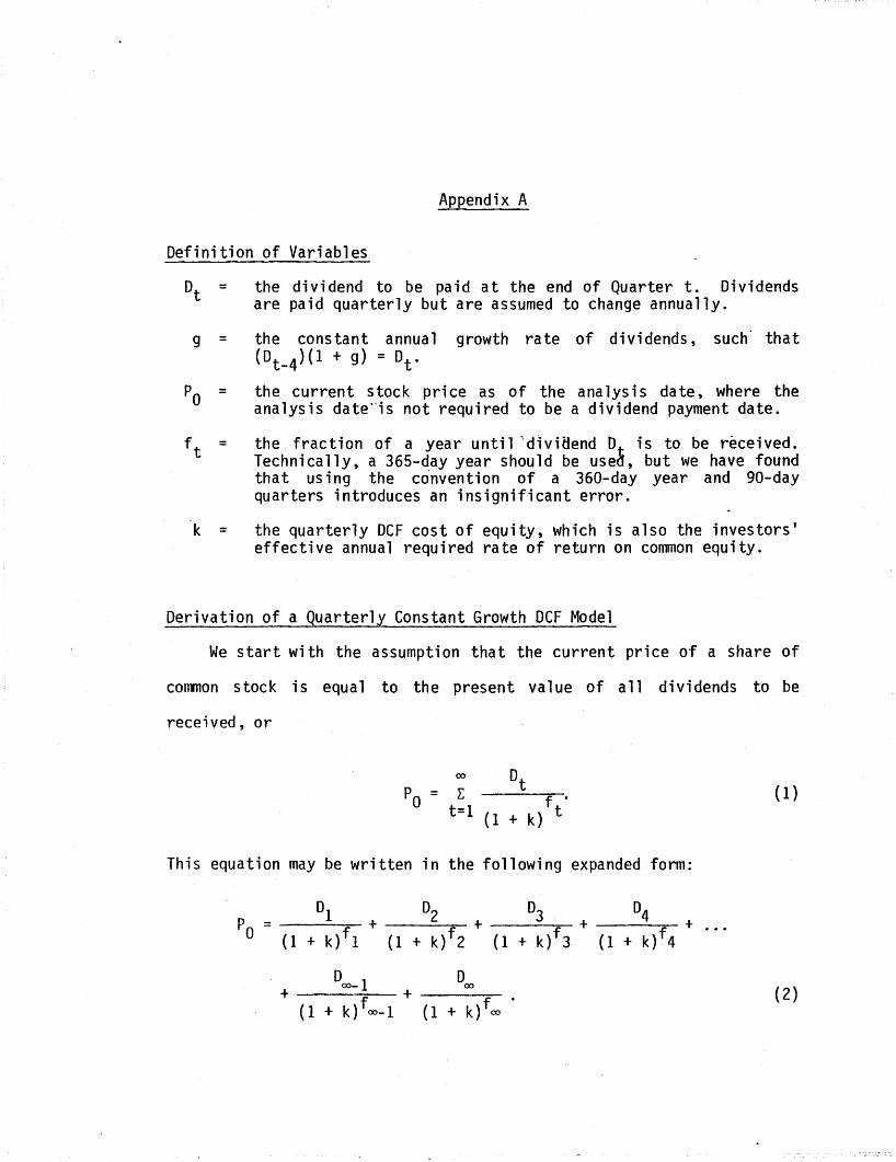
Appendix A

Definition of Variables

the dividend to be paid at the end of Quarter t. Dividendsare paid quarterly but are assumed to change annually.

g = the constant annual growth rate of dividends, such' that(Dt _4)(1 + g) = Dto

k =

the current stock pri ce as of the ana lys is da te, where theanalysis date'-is not required to be a dividend payment date.

the fraction of a year until "dlvi8end 0 is to be received.Technically, a 365-day year should be use~, but we have foundthat using the convention of a 360-day year and gO-dayquarters introduces an insignificant error.

the quarterly DCF cost of equity, which is also the investors'effective annual required rate of return on common equity.

Derivation of a Quarterly Constant Growth DCF Model

We start with the assumption that the current price of a share of

common stock is equal to the present value of all dividends to be

recei ved, or

00 Dt

Po = L f °t=1 t(1 + k)

This equation may be written in the following expanded form:

Doo

_ 1 Doo

+ ---=.--- + -------",-(1 + k)foo- 1 (1 + k)foo •

(1)

(2)

-A2-

Keeping in mind that 0t = 0t_4(1 + g), so 0t-4 = Dt/(l + g), we can

multiply both sides of Equation 2 by (1 + k)/(l + g) to obtain

1-f+ 00(1 + k) 4 +

1-f+ D

oo_4

(1 + k) 00 (3)

where D_ 3 through DO are the quarterly dividends already paid in the

previous year. If we now subtract Equation 2 from Equation 3, we will

obta in

1-f 1-f+ D_ 1(1 + k) 3 + DO(1 + k) 4

1-f 1-f- 000_3(1 + k) 00-3 - 000_2(1 + k) 00-2

1-f 1-f- D (1 + k) 00-1 - D (1 + k) 0000-1 00 (4)

If we assume that dividends are growing on an annual basis at a rate, g,

which is less than the investors' required rate of return, k, then the

last four terms on the right hand side of Equation 4 will approach zero

in the limit. Thus, Equation 4 may be reduced to

(5)

-A3-

If we now multiply both sides of Equation 5 by (1 + g)/(k - g), we will

obtain

Solving Equation 6 for k, we then obtain

1-f 1-f 1-f 1-f01(1 + k) 1 + D2(1 + k) 2 + D3(1 + k) 3 + D (1 + k) 4.

k = 4 + g, (7)Po

where 01 through 04 are the quarterly dividends expected to be received;- ;"

.:~,; ""

over the coming 12-month period. Note that t~e numerator of Equation 7

is simply the terminal (future) value of the quarterly dividends to be

received over the coming year, compounded forward to the end of the year

by the investors' required rate of return. As such, it takes into

consideration that investors will have the opportunity to reinvest these

dividends as they are received. If we allow the terminal value of these

quarterly dividends to be represented by TD1' then Equation 7 may be

restated as

ok =D + gP ,

o(8)

which is nothing more than a quarterly representation of the annual OCF

model.

If pricing takes place at a dividend payment date, where f 1 will be

equal to 0.25, then Equation 7 reduces to

D (1 + k)O.75 + 0 (1 + k)0.50 + 0 (1 + k)0.25 + D (1 + k)Ok = 1 2 3 4 + g. (9)

Po

'Rr

-A4-

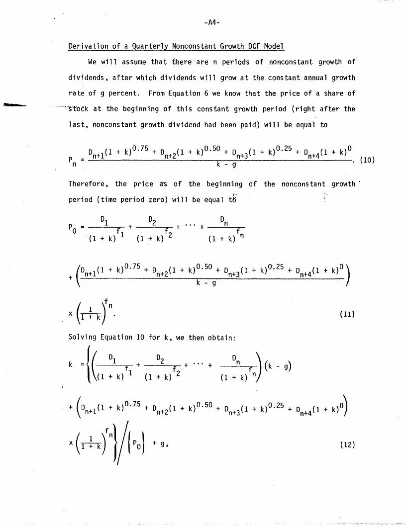
Derivation of a Quarterly Nonconstant Growth DCF Model

We will assume that there are n periods of nonconstant growth of

dividends, after which dividends will grow at the constant annual growth

rate of g percent. From Equation 6 we know that the price of a share of

"~~"'sTock at the beginning of this constant growth period (right after the

last, nonconstant growth dividend had been paid) will be equal to

Dn+1

(1 + k)0.75 + D (1 + k)0.50 + D (1 + k)0.25 + D (1 + k)Op n+2' n+3 n+4 (10.)n = k - g

Therefore, the pri ce a-s of the begi nni ng of the noncons tant growth·r·

period (time period zero) will be equal to

D2 Dnf + ••• + ----:::f~

(1 + k) 2 (1 + k) n

(D (1 + k)0.75 + D (1 + k)0.50 + D (1.+ k)0.25 + D (1 + k)O)

+ n+1 n+2 n+3 n+4k - g

(11)

Solving Equation 10 for k, we then obtain:

DI D2f + f + ... ++ k) 1 (1 + k) 2

1+ + g, (I2)

-A5-

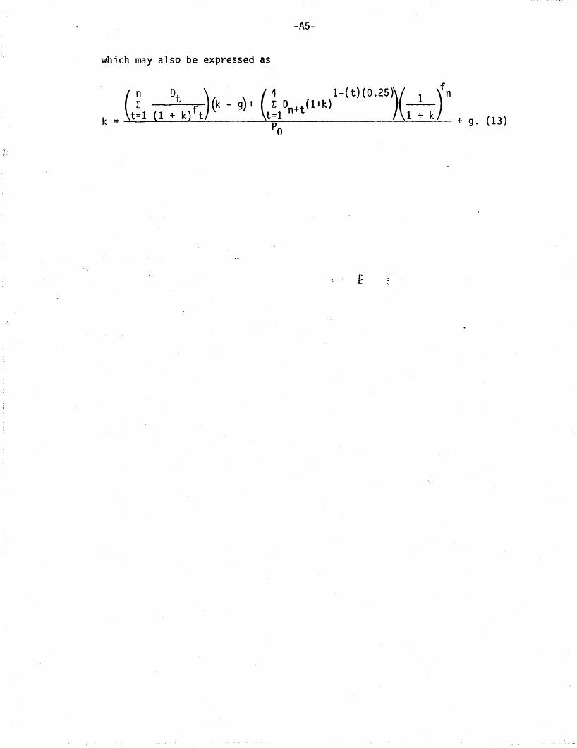
which may also be expressed as

(n Dt ) ( 4 1-(t)(O.25))~.)fnL (k - g) + E D (1+k)

k = t=1 (1 + k)f t t;1 n+t 1 + k + g. (13)a