1

Modern Methods of Estimating Biodiversity from Presence-AbsenceSurveys

Robert M. Dorazio1, U.S. Geological Survey and University of Florida, Department of Statistics,Gainesville, FL 32611, USA.Nicholas J. Gotelli, Department of Biology, University of Vermont, Burlington, VT 05405, USAAaron M. Ellison, Harvard Forest, Harvard University, Petersham, MA 01366, USA

1 Introduction

Communities of species are often sampled using so-called “presence-absence” surveys, wherein theapparent presence or absence of each species is recorded. Whereas counts of individuals can be usedto estimate species abundances, apparent presence-absence data are often easier to obtain in surveysof multiple species. Presence-absence surveys also may be more accurate than abundance surveys,particularly in communities that contain highly mobile species.

A problem with presence-absence data is that observations are usually contaminated by zeros thatstem from errors in detection of a species. That is, true zeros, which are associated with the absence ofa species, cannot be distinguished from false zeros, which occur when species are present in the vicinityof sampling but not detected. Therefore, it is more accurate to describe apparent presence-absencedata as detections and non-detections, but this terminology is seldom used in ecology.

Estimates of biodiversity and other community-level attributes can be dramatically affected byerrors in detection of each species, particularly since the magnitude of these detection errors generallyvaries among species (Boulinier et al. 1998). For example, bias in estimates of biodiversity arisingfrom errors in detection is especially pronounced in communities that contain a preponderance of rareor difficult-to-detect species. To eliminate this source of bias, probabilities of species occurrence anddetection must be estimated simultaneously using a statistical model of the presence-absence data.Such models require presence-absence surveys to be replicated at some – but not necessarily all – of thelocations selected for sampling. Replicate surveys can be obtained using a variety of sampling protocols,including repeated visits to each sample location by a single observer, independent surveys by differentobservers, or even spatial replicates obtained by placing clusters of quadrats or transects within asample location. Information in the replicated surveys is crucial because it allows species occurrencesto be estimated without bias by using a model-based specification of the observation process, whichaccounts for the errors in detection that are manifest as false zeros.

Several statistical models have been developed for the analysis of replicated, presence-absence data.Each of these models includes parameters for a community’s incidence matrix (Gotelli 2000, Colwellet al. 2004), which contains the binary occupancy state (presence or absence) of each species at eachsample location. The incidence matrix is only partially observed owing to species- and location-specificerrors in detection; however, the incidence matrix can be estimated by fitting these models to thereplicated, presence-absence data. Therefore, any function of the incidence matrix – including speciesrichness, alpha diversity, and beta diversity (Magurran 2004)– also can be estimated using these models.

Models for estimating species richness – and other measures of biodiversity – from replicated,presence-absence data were first developed by Dorazio and Royle (2005) and Dorazio et al. (2006).By including spatial covariates of species occurrence and detection probabilities in these models, Keryand Royle (2009) and Royle and Dorazio (2008) estimated the spatial distribution (or map) of speciesrichness of birds in Switzerland. Similarly, Zipkin et al. (2010) showed that this approach can beused to quantify and assess the effects of conservation or management actions on species richness

1Correspondence: University of Florida, Department of Statistics, 429 McCarty Hall C, Gainesville, FL 32611-0339,USA. E-mail: bdorazio@usgs.gov

2

and other community-level characteristics. More recently, statistical models have been developed toestimate changes in communities from a temporal sequence of replicated, presence-absence data. Inthese models the dynamics of species occurrences are specified using temporal variation in covariatesof occurrence (Kery et al. 2009a) or using first-order Markov processes (Russell et al. 2009, Dorazioet al. 2010, Walls et al. 2011), wherein temporal differences in occurrence probabilities are specifiedas functions of species- and location-specific colonization and extinction probabilities. The latter classof models, which includes the former, is extremely versatile and may be used to confront alternativetheories of metacommunity dynamics (Leibold et al. 2004, Holyoak and Mata 2008) with data orto estimate changes in biodiversity. For example, Dorazio et al. (2010) estimated regional levels ofbiodiversity of butterflies in Switzerland using a model that accounted for seasonal changes in speciescomposition associated with differences in phenology of flight patterns among species. Russell et al.(2009) estimated the effects of prescribed forest fire on the composition and size of an avian communityin Washington.

In the present paper we analyze a set of replicated, presence-absence data that previously wasanalyzed using statistical models that did not account for errors in detection of each species (Gotelliand Ellison 2002). Our objective is to illustrate the inferential benefits of using modern methods toanalyze these data. In the analysis we model occurrence probabilities in assemblages of ant speciesas a function of large-scale, geographic covariates (latitude, elevation) and small-scale, site covariates(habitat area, vegetation composition, light availability). We fit several models, each identified bya specific combination of covariates, to assess the relative contribution of these potential sources ofvariation in species occurrence and to estimate the effect of these contributions on geographic differencesin ant species richness and other measures of biodiversity. We also provide the data and source codeused in our analysis to allow comparisons between our results and those obtained using alternativemethods of analysis.

2 Study Area and Sampling Methods

2.1 Ant sampling

The data in our analysis were obtained by sampling assemblages of ant species found in New Englandbogs and forests. The initial motivation for sampling was to determine the extent of the distribution ofthe apparent bog-specialist, Myrmica lobifrons, in Massachusetts and Vermont. Bogs are not commonlysearched for ants, but in 1997 we had identified M. lobifrons as a primary component of the diet ofthe carnivorous pitcher plant, Sarracenia purpurea, at Hawley Bog in western Massachuestts. This wasthe first record for M. lobifrons in Massachusetts. At the time the taxonomic status of this species wasbeing re-evaluated (Francoeur 1997), and it was largely unknown in the lower (contiguous) 48 states ofthe United States. In addition to our interest in M. lobifrons, we also wanted to explore whether bogsharbored a distinctive ant fauna or whether the ant faunas of bogs were simply a subset of the antspecies found in the surrounding forests. Thus, at each of the sites selected for sampling, we surveyedants in the target bog and in the upland forest adjacent to the bog (Gotelli and Ellison 2002).

At each of 22 sample sites, we established two 8 × 8 m sampling grids, each containing 25 evenlyspaced pitfall traps. One sampling grid was located in the center of the bog; the other was locatedwithin intact forest 50-500 m away from the edge of the bog. Each pitfall trap consisted of a 180-mlplastic cup (95 mm in diameter) that was filled with 20 ml of dilute soapy water. Traps were buriedso that the upper lip of each trap was flush with the bog or forest-soil surface, and left in place for 48hours during dry weather. At the end of the 48 hours, trap contents were collected, immediately fixedwith 95% ethanol, and returned to the laboratory where all ants were removed and identified to species.Traps were sampled twice in the summer of 1999, and the time between each sampling period was 6weeks (42 days); therefore, we consider the two sampling periods as early- and late-summer replicates.

3

Locations of traps were flagged so that pitfall traps were placed at identical locations during the twosampling periods.

2.2 Measurement of site covariates

The geographic location (latitude (LAT) and longitude (LON)) and elevation (ELEV, meters abovesea level) of each bog and forest sample site was determined using a Trimble Global Positioning System(GPS). At each forest sample site we also estimated available light levels beneath the canopy usinghemispherical canopy photographs, which were taken on overcast days between 10:00 AM and and 2:00PM at 1 m above ground level with an 8 mm fish-eye lens on a Nikon F-3 camera. Leaf area index(LAI, dimensionless) was determined from the subsequently digitized photographs using HemiViewsoftware (Delta-T, Cambridge, UK). Because there was no canopy over the bog, the LAI of each bogwas assigned a value of zero.

To compute a global site factor (GSF, total solar radiation) for each forest sample site (Rich et al.1993), we summed weighted values of direct site factor (DSF, total direct beam solar radiation) andindirect site factor (total diffuse solar radiation). GSF values are expressed as a percentage of totalpossible solar radiation (i.e., above the canopy) during the growing season (April through October),corrected for latitude and solar track. The GSF of each bog was assigned a value of one.

Digital aerial photographs were obtained for each sampled bog from state mapping authorities,or, when digital photographs were unavailable (five sites), photographic prints (from USGS-EROS)were scanned and digitized. Aerial photographs were used to construct a set of data layers (Arc-ViewGIS 3.2) from which bog area (AREA) was calculated. The area of the surrounding forests was notmeasured, as the forest was generally continuous for at least several km2 around each bog.

3 Statistical Analysis

We analyzed the captures of ant species observed at our sample sites using a modification of the multi-species model of occurrence and detection that includes site-specific covariates (Royle and Dorazio2008, Kery and Royle 2009). This modification allows a finite set of candidate models to be specifiedand fit to the data simultaneously such that prior beliefs in each model’s utility can be updated (usingBayes’ rule) to compute the posterior probability of each model. The resulting set of posterior modelprobabilities can be used to select a single (“best”) model for inference or to estimate scientificallyrelevant quantities while averaging over the posterior uncertainty of the models (Draper 1995).

To compare our results with previous analyses (Gotelli and Ellison 2002), we analyzed the dataobserved in bogs and forests separately. These two habitats are sufficiently distinct that differencesin species occurrence – and possibly capture rates – are expected a priori. Furthermore, the potentialcovariates of occurrence differ between the two habitats, adding another reason to analyze the bog andforest data separately.

3.1 Hierarchical model of species occurrence and capture

We summarize here the assumptions made in our analysis of the ant captures. Let yik ∈ 0, 1, . . . , Jkdenote the number of pitfall traps located at site k that contained the ith of n distinct species ofants captured in the entire sample of R = 22 sites. At each site 25 pitfall traps were deployedduring each of 2 sampling periods (early- and late-season replicates); therefore, the total number ofreplicate observations per site was constant (Jk = 50). While constant replication among sites simplifiesimplementation of the model, it is not required. However, it is essential that Jk > 1 for some (ideallyall) sample sites because information from within-site replicates allows both occurrence and detection

4

probabilities to be estimated for each species. In the absence of this replication these two parametersare confounded.

The observed data form an n×R matrix Y obs of pitfall trap frequencies, so that rows are associatedwith distinct species and columns are associated with distinct sample sites. Note that n, the numberof distinct ant species observed among all R sample sites, is a random outcome. In the analysis wewant to estimate the total number of species N that are present and vulnerable to capture. AlthoughN is unknown, we know that n ≤ N , i.e., we know that the number of species observed in the samplesprovides a lower bound for an estimate of N .

To estimate N , we use a technique called parameter-expanded data augmentation (Dorazio et al.2006, Royle and Dorazio 2011), wherein rows of all-zero trap frequencies are added to the observeddata Y obs and the model for the observed data is appropriately expanded to analyze the augmenteddata matrix Y = (Y obs,0). The technical details underlying this technique are described by Royleand Dorazio (2008, 2011), so we won’t repeat them here. Briefly, however, the idea is to embed theunobserved, all-zero trap frequencies of the N − n species in the community within a larger data setof fixed, but known size (say, M species, where M > N) for the purpose of simplifying the analysis.The conventional model for the community of N species is necessarily modified so that each of theM − n rows of augmented data can be estimated as either belonging to the community of N species(and containing sampling zeros) or not (and containing structural zeros). In particular, we add avector of parameters w = (w1, . . . , wM ) to the model to indicate whether each species is a member ofthe community (w = 1) or not (w = 0). The elements of w are assumed to be independentally andidentically distributed (iid) as follows:

wiiid∼ Bernoulli(Ω)

where the parameter Ω denotes the probability that a species in the augmented data set is a memberof the community of N species that are present and vulnerable to capture. Note that the community’sspecies richness N is not a formal parameter of the model. Instead, N is a derived parameter to becomputed as a function of w as follows: N =

∑Mi=1wi. Therefore, estimation of Ω and w is essentially

equivalent to estimation of N (Royle and Dorazio 2011).The incidence matrix of the community (Gotelli 2000, Colwell et al. 2004) is a parameter of the

model that is embedded in an M × R matrix of parameters Z, whose elements indicate the presence(z = 1) or absence (z = 0) of species i at sample site k. Although Z is treated as a random variableof the model, each element associated with species that are not members of the community is equal tozero because zik is defined conditional on the value of wi as follows:

zik|wi ∼ Bernoulli(wiψik) (1)

where ψik denotes the probability that species i is present at sample site k. Thus, if species i isnot a member of the community, then wi = 0 and Pr(zik = 0|wi = 0) = 1; otherwise, wi = 1 andPr(zik = 1|wi = 1) = ψik. For purposes of computing estimates of community-level characteristics, Zmay be treated as the incidence matrix itself because the M −N rows associated with species not inthe community contain only zeros and make no contribution to the estimates.

The matrix of augmented data Y and the parameters Z and w may be conceptualized as character-istics of a supercommunity of M species (Table 1). This supercommunity includes N species that aremembers of the community vulnerable to sampling and M −N other species that are added to simplifythe analysis. The parameters Z and w are paramount in terms of estimating measures of biodiversity.We have shown already that estimates of w are used to compute estimates of species richness N (ameasure of gamma diversity). Similarly, Z may be used to estimate measures of alpha diversity, betadiversity, and other community-level characteristics. For example, summing the columns of Z yieldsthe number of species present at each sample site (alpha diversity). Similarly, different columns of

5

Z may be compared to express differences in species composition among sites (beta diversity). Forexample, the Jaccard index, a commonly used measure of beta diversity (Anderson et al. 2011), iseasily computed from Z. The Jaccard index requires the number of species from two distinct sites, sayk and l, that occur at both sites. Off-diagonal elements of the R×R matrix Z ′Z contain the numbersof species shared between different sites. Therefore, the proportion of all species present at two sites,say k and l, that are common to both sites is

Jkl =z′kzl

z′k1 + z′l1− z′kzl

where 1 denotes a M ×1 vector of ones, and zk and zl denote the kth and lth columns of Z. Note thatJkl is a measure of the similarity in species present at sites k and l; its complement, 1−Jkl, correspondsto the dissimilarity – or beta diversity – between sites.

In Section 4 we provide estimates of gamma diversity, alpha diversity, and beta diversity in ouranalyses of the ant data sets. In these analyses we assume that the community of ants contains amaximum of M = 75 species in the forest habitat and a maximum of M = 25 species in the boghabitat. The lower maximum is based on five years of collecting ants in New England bogs thatyielded only 21 distinct species (Ellison and Gotelli, personal observations). The total number of antspecies in all of New England is somewhere between 130 and 140 (Ellison et al. 2012); however, many ofthese species are field or grassland species, and six species, which are not indigenous to New England,are restricted mainly to warm indoors. By excluding these species and those found only in bogs, weobtain the upper limit for the number of ant species in the forest habitat.

3.1.1 Modeling species occurrence probabilities

Equation 1 implies that each element of the incidence matrix is assumed to be independent given ψik,the probability of occurrence of species i at sample site k. Let xk = (xk1, xk2, . . . , xkp) denote theobserved value of p covariates at site k. We assume that each of these covariates potentially affects thespecies-specific probability of occurrence at site k. Naturally, the effects of these covariates may differamong species, so their contributions are modeled on the logit-scale as follows:

logit(ψik) = b0i + δ1b1ix1k + · · ·+ δpbpixpk (2)

where b0i denotes a logit-scale, intercept parameter for species i and bli denotes the effect of covariatexl on the probability of occurrence of species i (l = 1, . . . , p). If each covariate is centered and scaledto have zero mean and unit variance, b0i denotes the logit-scale probability of occurrence of species i atthe average value of the covariates. This scaling of covariates also improves the stability of calculationsinvolved in estimating bi = (b0i, b1i, . . . , bpi).

The additional parameter δ = (δ1, . . . , δp) in Eq. 2 is used to specify whether each covariate is(δ = 1) or is not (δ = 0) included in the model. Specifically, we assume

δliid∼ Bernoulli(0.5)

which implies an equal prior probability (0.5p) for each of the 2p distinct values of δ. This approach,originally developed by Kuo and Mallick (1998), allows several regression models to be consideredsimultaneously and yields the posterior distribution of δ. After all models have been considered (asdescribed in Section 3.2), the posterior probability Pr(δ|Y ,X) of each model (vis a vis, each distinctvalue of δ) can be computed. In our analyses the model with the highest posterior probability is usedto compute estimates of species occurrence and biodiversity.

6

3.1.2 Modeling species captures

We assume a relatively simple model of the pitfall trap frequencies yik, owing to the simplicity of oursampling design. Specifically, we assume that if ants of species i are present at site k (i.e., zik = 1),their probability of capture pik is the same in each of the Jk replicated traps. This assumption impliesthe following binomial model of the pitfall trap frequencies:

yik|zik ∼ Binomial(Jk, zikpik)

where pik denotes the conditional probability of capture of species i at site k (given zik = 1). Notethat if species i is absent at site k, then Pr(yik = 0|zik = 0) = 1. In other words, if a species is absentat sample site k, then none of the Jk pitfall traps will contain ants of that species under our modelingassumptions.

None of the covariates observed in our samples is thought to be informative of ant capture prob-abilities; therefore, rather than using a logistic-regression formulation of pik (as in Eq. 2), we assumethat the logit-scale probability of capture of each species is constant:

logit(pik) = a0i

at each of the R sample sites.

3.1.3 Modeling heterogeneity among species

In order to estimate the occurrences of species not observed in any of our traps, a modeling assumptionis needed to specify a relationship among all species-specific probabilities of occurrence and detection.Therefore, we assume that the ant species in each community are ecologically similar in the sense thatthese species are likely to respond similarly, but not identically, to changes in their environment orhabitat, to changes in resources, or to changes in predation. The assumption of ecological similarityseems reasonable for the species we sampled owing to their overlapping diets, habitats, and life historycharacteristics. As a point of emphasis, we would not assume ecological similarity if our assemblage hadincluded species of tigers and mice! The idea of ecological similarity has been used previously to analyzeassemblages of songbird, butterfly, and amphibian species (Dorazio et al. 2006, Kery et al. 2009b, Wallset al. 2011); however, this idea is not universally applicable. For example, if the occurrence of one speciesdepends on the presence or absence of another species (as might occur between a predator and preyspecies or between strongly competing species), then ecological similarity would not be a reasonableassumption. In this case a model must be formulated to specify the pattern of co-occurrence thatarises from interspecific interactions (MacKenzie et al. 2004, Waddle et al. 2010). The formulation ofstatistical models for inferring interspecific interactions in communities of species is an important anddeveloping area of research (Dorazio et al. 2010).

In assemblages of ecologically similar species, it seems reasonable to use distributional assumptionsto model unobserved sources of heterogeneity in probabilities of species occurrence and detection. Forexample, occurrence probabilities may be low for some species (the rare ones) and high for others,but all species are related in the sense that they belong to a larger community of ecologically similarspecies. By modeling the heterogeneity among species in this way, the data observed for any individualspecies influence the parameter estimates of every other species in the community. In other words,inferences about an individual species do not depend solely on the observations of that species becausethe inferences borrow strength from the observations of other species. A practical manifestation ofthis multispecies approach is that the estimate of a parameter (e.g., occurrence probability) of a singlespecies reflects a compromise between the estimate that would be obtained by analyzing the data fromeach species separately and the average value of that parameter among all species in the community.In the statistical literature this phenomenon is called “shrinkage” (Gelman et al. 2004) because each

7

species-specific estimate is shrunk in the direction of the estimated average parameter value. Of course,the amount of shrinkage depends on the relative amount of information about the parameter in theobservations of each species versus the information about the mean value of that parameter. Animportant benefit of shrinkage is that it allows parameters to be estimated for a species that is detectedwith such low frequency that its parameters could otherwise not be estimated. Such species are oftenthe rarest members of the community, and it is crucial that these species be included in the analysisto ensure that estimates of biodiversity are accurate.

In the present analysis we use a normal distribution[b0ia0i

]iid∼ Normal

([β0α0

],

[σ2b0 ρ σb0σa0

ρ σb0σa0 σ2a0

]), (3)

to specify the variation in occurrence and detection probabilities among ant species. The parametersσb0 and σa0 denote the magnitude of this variation, and ρ parameterizes the extent to which speciesoccurrence and detection probabilities are correlated.

We also use the normal distribution to specify variation among the species-specific effects of covari-

ates on occurrence. Specifically, we assume bliiid∼ Normal(βl, σ

2bl

) (for l = 1, . . . , p), so that the effectsof different covariates are assumed to be mutually independent and uncorrelated.

3.2 Parameter estimation

The hierarchical model described in Section 3.1 would be impossible to fit using classical methods owingto the high-dimensional and analytically intractable integrations involved in evaluating the marginallikelihood function. We therefore adopted a Bayesian approach to inference and used Markov chainMonte Carlo methods (Robert and Casella 2004) to fit the model. In the appendix (Section 7) wedescribe our choice of prior distributions for the model’s parameters. We also provide the data and thecomputer code that was used to calculate the joint posterior distribution of the model’s parameters.All parameter estimates and credible intervals are based on this distribution.

4 Results

4.1 Effects of covariates on species occurrence

The posterior model probabilities calculated in our analysis of forest and bog data sets are only mildlysensitive to our choice of priors for the logit-scale parameters of the model (Table 2). Recall that theseparameters are of primary interest in assessing the relative contributions of geographic- and site-levelcovariates. Regardless of the prior distribution used (Uniform or Jeffreys’ (see appendix)), the modelwith highest probability includes all four covariates (LAT, LAI, GSF, ELEV) in the analysis of dataobserved at forest sample sites and a single covariate (ELEV) in the analysis of data observed at bogsample sites. However, the model without any covariates has nearly equal probability to the favoredmodel of the bog data, and the combined probability of these two models far exceeds the probabilitiesof all other models. These results suggest that occurrence probabilities of ant species found in the boghabitat are not strongly influenced by the LAT or AREA covariates, either alone or in combinationwith other covariates.

Each of the four covariates used to model species occurrences in the forest habitat has an average,negative effect on occurrence probabilities. Estimates of βl and 95% credible intervals are as follows:LAT, -0.717 (−1.217,−0.257); LAI, -0.850 (−1.302,−0.440); GSF, -0.494, (−0.916,−0.098); ELEV,-0.662 (−1.014,−0.339). However, as illustrated in Figure 1, there is considerable variation amongspecies in the magnitude of these effects . Similarly, the estimated occurrence probabilities of antsin the bog habitat decrease with ELEV (β1 = −0.500 (−1.019,−0.098)), and there is considerablevariation among species (σb1 = 0.320 (0.014, 1.000)) in the magnitude of ELEV effects.

8

4.2 Estimates of biodiversity

Our pitfall trap surveys revealed n = 34 distinct species of ants at the forest sample sites and n = 19species at the bog sample sites. The estimated species richness of ants found in the forest habitat(N = 43 (95% interval = (37, 70)) is nearly twice the estimated richness of ants in the bog habitat(N = 25 (95% interval = (21, 25)); however, the estimate of forest ant richness is relatively impreciseand the estimate of bog ant richness is strongly influenced by the upper bound (M = 25 species).

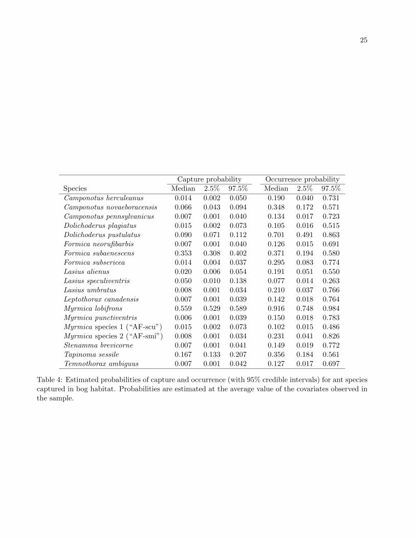
The numbers of species found in forest and bog communities are perhaps better compared usingestimates of species richness at the sample sites. These measures of alpha diversity are plotted againsteach site’s elevation in Figure 2, which also includes the number of ant species actually captured. Theestimated richness at sites in the forest habitat usually exceeds that at sites in the bog habitat whenthe effects of elevation on species occurrences are taken into account. Note also that a site’s estimatedspecies richness can be much higher than the numbers of species captured because capture probabilitiesare much lower than one for most species (Tables 3 and 4).

Site-specific estimates of beta diversity between bog and forest communities of ants are relativelyhigh, ranging from 0.71 to 1.0 (Figure 3). These estimates also generally exceed the beta diversities be-tween ants from different sites within each habitat (Figure 4), adding further support for the hypothesisthat composition of ant species differs greatly between forest and bog habitats.

5 Discussion

5.1 Analysis of ant species

It is interesting to compare the results of our analyses with the results reported by Gotelli and Ellison(2002), who analyzed the same data but did not account for errors in detection of species. Gotelli andEllison (2002) used linear regression models to estimate associations between the number of observedspecies (which was referred to as “species density”) and environmental covariates. For bog ants Gotelliand Ellison (2002) reported a significant association between species density and latitude (P = 0.041)and a marginally significant association between species density and vegetation structure (as measuredby the first principal-component score; P = 0.081). Collectively, these two variables accounted forabout 30% of the variation in species density. In the present analysis of the bog data, the bestfitting model included the effect of a single covariate (ELEV) on ant species occurrence probabilities,though a model without any covariates was a close second (Table 2). In the analysis of forest antsGotelli and Ellison (2002) reported significant positive associations between species density and the firsttwo principal components of vegetation structure, and they reported significant negative associationsbetween species density and four other covariates (LAT, LAI, GSF, and ELEV). Collectively, these sixregressors accounted for 83% of the variation in species density. In the present analysis of forest data,the best-fitting model included the effects of four covariates (LAT, LAI, GSF, and ELEV), and theestimated effects of these covariates were all significantly negative, which agrees qualitatively with theregression results of Gotelli and Ellison (2002), though principal components of vegetation structurewere not included in the present analysis.

In comparing the results obtained using the linear regression model (Gotelli and Ellison 2002) andthe hierarchical model of species occurrences and captures, we note that while both models revealedthe same set of negative predictors of ant occurrence in forest habitat (Figure 1), the regression model’sassociations between species density of bog ants and two predictors (latitude and vegetation structure)are not supported by the hierarchical model. Part of the difference in these results may be attributedto the fact that slightly different data sets were used in the two analyses. Species detected usingtuna baits, hand collections, and leaf-litter sorting (in forest habitats) were included in the regressionanalysis, whereas only species captured in pitfall traps were used in the present analysis. However, thesedifferences in data are relatively minor because the alternative sampling methods used by Gotelli and

9

Ellison (2002) added only a few rare species to their analysis. Instead, we believe the different resultsstem primarily from differences in the underlying assumptions of these two models. The regressionmodel assumes (1) that the effects of environmental covariates are identical for each species and arelinearly related to species density and (2) that residual errors in species density are normally distributedand do not distinguish between measurement errors and heterogeneity among species in their responseto covariates. In contrast, the hierarchical model assumes that the effects of environmental covariatesdiffer among species (Figure 1) and that occurrence probabilities and capture probabilities can beestimated separately for each species (Tables 3 and 4) owing to the replicated sampling at each site.

The estimated probabilities of occurrence and capture of each species are of great interest in them-selves and highlight differences in species compositions between ants found in bog and forest habitats.For example, the forest species with the highest occurrence probability was Aphaenogaster rudis (speciescomplex) (ψ = 0.779). This species is taxonomically unresolved and currently includes a complex ofpoorly differentiated species across its geographic range (Umphrey 1996). Myrmica punctiventris hadthe second highest occurrence probability (ψ = 0.739). Both of these species are characteristic of forestant assemblages in New England. A. rudis (species complex) was never captured in bogs and theoccurrence probability of M. punctiventris in bogs was only 0.150, almost a fivefold difference betweenthe two habitats.

In bogs the highest occurrence probabilities were estimated for the bog specialist, Myrmica lob-ifrons (ψ = 0.916), and for Dolichoderus pustulatus (ψ = 0.701), a generalist species that sometimesbuilds carton nests in dead leaves of the carnivorous pitcher plant Sarracenia purpurea (A. Ellison andN. Gotelli, personal communication). Occurrence probabilities of these species in forests were only0.299 (M. lobifrons) and 0.042 (D. pustulatus), a 3- to 16-fold difference. These pronounced differencesin the occurrence probabilities of the most common species in each habitat suggest that the two habi-tats support distinctive ant assemblages, a conclusion also supported by the relatively high estimatesof beta diversity between habitats (Figure 3).

Although occurrence and capture probabilities were positively correlated among species (Figure 5),a few rare forest species (Formica subintegra and Formica subsericea) had relatively high captureprobabilities. In the forest habitat the two species with the highest capture probabilities were F.subsericea (p = 0.248) and Myrmica punctiventris (p = 0.248). In bogs these species had captureprobabilities of only 0.014 (F. subsericea) and 0.006 (M. punctiventris), a 17- to 41-fold difference.The two species with the highest capture probabilities in the bog habitat were Myrmica lobifrons(p = 0.559), the bog specialist, and Formica subaenescens (p = 0.353). In the forest habitat thesespecies had capture probabilities of only 0.056 (M. lobifrons) and 0.051 (F. subaenescens), a 7- to9-fold difference.

The estimated probabilities of occurrence of most species in the forest habitat decreased with lat-itude (Figure 1), which is consistent with previous regression analyses of species density (Gotelli andEllison 2002, figure 1). However, the occurrence probabilities of three species (Camponotus herculeanus,Lasius alienus, and Myrmica detritinodis) significantly increased with latitude. Two of these species,C. herculeanus and M. detritinodis, are boreal, cold-climate specialists (Ellison et al. 2012), whereasL. alienus has a more widespread distribution. Under climate change scenarios of increasing temper-atures at high latitudes, species whose occurrence probabilities currently increase with latitude mightdisappear from New England as their ranges shift northward; other species in the assemblage mightshow no change in distribution, or might increase in occurrence.

To summarize the comparisons between our results and those reported by Gotelli and Ellison (2002),we note that within-site replication of presence-absence surveys allowed us to estimate species-specificprobabilities of capture and occurrence and species-specific effects of environmental covariates. Theseresults represent a considerable advance over traditional regression analyses of observed species density.Using a hierarchical approach to model building, we were able to infer sources of variation in measuresof biodiversity – such as the effect of elevation on site-specific species richness (Figure 2) and the

10

effect of habitat on beta diversity (Figure 3) – and to determine how these community-level patternswere related to differences in occurrence of individual species. Although many macroecological datasets collected at large spatial scales do not include within-site replicates, regional studies often usereplicated sampling grids of traps or baits (Gotelli et al. 2011) that are ideal for the kind of analysiswe have described. We therefore recommend that within-site replication be used in presence-absencesurveys of communities, particularly when surveys are undertaken to assess levels of biodiversity.

5.2 Benefits and challenges of hierarchical modeling

Our analysis of the ant data illustrates the benefits of using hierarchical models to estimate measures ofbiodiversity and other community-level characteristics. By adopting a hierarchical approach to modelbuilding, an analyst actually specifies two models: one for the ecologically relevant parameters (or statevariables) that are usually of primary interest but are not directly observable, and a second model forthe observed data, which are related to the ecological parameters but are influenced also by samplingmethods and sampling errors. This dichotomy between models of ecological parameters and modelsof data is extremely useful and has been exploited to solve a variety of inference problems in ecology(Royle and Dorazio 2008).

In our hierarchical model of replicated, presence-absence surveys, the parameter of primary eco-logical interest is the community’s incidence matrix. This matrix is only partially observable becausea species may be present at a sample location but not observed in the surveys. We use a binomialsampling model to specify the probability of detection (or capture) of each species and thereby toaccount for detection errors in the observed data. In this way estimates of the community’s incidencematrix are automatically adjusted for the imperfect detectability of each species.

In our approach, measures of biodiversity are estimated indirectly as functions of the estimatedincidence matrix of the community. Thus, species richness and measures of alpha or beta diversitydepend on a set of model-based estimates of species- and site-specific occurrences. This approachdiffers considerably with classes of statistical models wherein species richness is treated as a singlerandom variable – usually a discrete random variable – that represents the aggregate contribution ofall species in the community. This “top-down” view of a community may yield incorrect inferencesif heterogeneity in detectability exists among species or if the effects of environmental covariates onoccurrence differ among species, as illustrated in our analysis of the ant data.

The inferential benefits of using hierarchical models to estimate measures of biodiversity are not free.As described earlier, the price to be paid for the ability to estimate probabilities of species occurrenceand species detection is replication of presence-absence surveys within sample locations. In our opinionthe improved understanding acquired in modeling the community at the level of individual species andthe versatility attained by having accurate estimates of a community’s incidence matrix far outweighthe cost of additional sampling. That said, there are other, perhaps less obvious, costs associatedwith these hierarchical models. Specifically, estimates of species richness and other community-levelparameters may be sensitive to the underlying assumptions of these models, and these assumptions canbe difficult to test using standard goodness-of-fit procedures. For example, the choice of distributions formodeling heterogeneity among species or sites may exert some influence on estimates of species richness.We assumed a bivariate normal distribution for the distribution of logit-scale, mean probabilities ofoccurrence and detection, but other distributions – even multimodal distributions – also might beuseful. In single-species models of replicated, presence-absence surveys, estimates of occurrence aresensitive to the distribution used to specify heterogeneity in detection probabilities among samplesites (Royle 2006, Dorazio 2007); therefore, similar sensitivity can be expected in multispecies models,though this aspect of model adequacy has not been rigorously explored.

Another assumption of our model that is difficult to test is absence of false-positive errors in de-tection. In other words, if a species is detected (or captured), we assume that its identify is known

11

with certainty. However, in surveys of avian or amphibian communities where species are detectedby their vocalizations, misidentifications of species can and do occur (Simons et al. 2007, McClin-tock et al. 2010a,b). These misidentifications are even more common in circumstances where surveysare conducted by volunteers whose identification skills are highly variable (Genet and Sargent 2003).If ignored, false-positive errors in detection induce a positive bias in estimates of species occurrencebecause species are incorrectly “detected” at sites where they are absent. While it is possible to con-struct statistical models of presence-absence data that include parameters for both false-positive andfalse-negative detection errors (Royle and Link 2006), these models are prone to identifiability prob-lems. To reduce these problems, Royle and Link (2006) recommended that the model’s parametersbe constrained to ensure that estimates of misclassification probabilities are lower than estimates ofdetection probabilities. This constraint, though sensible, does not provide a solution when the prob-abilities of misclassification and detection are nearly equal (Royle and Link 2006, McClintock et al.2010b). The development of statistical models of species occurrence that include both false-positiveand false-negative errors in detection, as well as unobserved sources of heterogeneity in both occurrenceand detection probabilities, is an active area of research owing to the difficulties associated with auraldetection methods.

The conceptual framework described in this paper is broadly applicable in ecological research andin assessments of biodiversity. Hierarchical, statistical models of multispecies, presence-absence datacan be used to estimate current levels of biodiversity, as illustrated in our analysis of the ant data, or toassess changes (e.g., trends) in communities over time (Kery et al. 2009a, Russell et al. 2009, Dorazioet al. 2010, Walls et al. 2011). The models of community change are especially relevant in ecologicalresearch because they provide an analytical framework wherein data may be used to confront alternativetheories of metacommunity dynamics (Leibold et al. 2004, Holyoak and Mata 2008). Although a fewclasses of statistical models have been developed to infer patterns of co-occurrence among species(MacKenzie et al. 2004, Waddle et al. 2010), models for estimating the dynamics of interacting species(e.g., competitors or predators) from replicated, presence-absence data have not yet been formulated.Such models obviously represent an important area of future research.

6 Acknowledgments

Collection of the original ant dataset was supported by NSF grants 98-05722 and 98-08504 to AMEand NJG, respectively, and by contract MAHERSW99-17 from the Massachusetts Natural Heritageand Endangered Species Program to AME. Additional support for AME’s and NJG’s research on thedistribution of ants in response to climatic change is provided by the U.S. Department of Energythrough award DE-FG02-08ER64510. The statistical modeling and analysis was conducted as a partof the Binary Matrices Working Group at the National Institute for Mathematical and BiologicalSynthesis, sponsored by the National Science Foundation, the U.S. Department of Homeland Security,and the U.S. Department of Agriculture through NSF Award #EF-0832858, with additional supportfrom The University of Tennessee, Knoxville.

Any use of trade, product, or firm names is for descriptive purposes only and does not implyendorsement by the U.S. Government.

7 Appendix: Technical Details

7.1 Model fitting and software

Here we describe methods for fitting our hierarchical model using the Markov chain Monte Carlo(MCMC) algorithms implemented in the software package, JAGS (Just Another Gibbs Sampler), whichis freely available at the following web site: http://mcmc-jags.sourceforge.net. This software

12

allows the user to specify a model in terms of its underlying assumptions, which include the distributionsassumed for the observed data and the model’s parameters. The latter distributions include priors,which are needed, of course, to conduct a Bayesian analysis of the data (see below). Part of the reasonfor the popularity of JAGS is that it allows the model to be specified and fitted without requiring theuser to derive the MCMC sampling algorithms used in computing the joint posterior. That said, naiveuse of JAGS may yield undesirable results, and some experience is needed to ensure the accuracy ofthe results.

We prefer to execute JAGS remotely from R (R Development Core Team 2004) using functionsdefined in the R package RJAGS (http://mcmc-jags.sourceforge.net). In this way R is used toorganize the data, to provide inputs to JAGS, and to receive outputs (results) from JAGS. However,the model’s distributional assumptions must be specified in the native language of JAGS. The datafiles and source code needed to fit our model are provided below.

In our analysis of each data set, the posterior was calculated by initializing each of 5 Markov chainsindependently and running each chain for a total of 250,000 draws. The first 50,000 draws of eachchain were discarded as “burn-in”, and every 50th draw in the remainder of each chain was retainedto form the posterior sample. Based on Gelman-Rubin diagnostics of the model’s parameters (Brooksand Gelman 1998), this approach appeared to produce Markov chains that had converged to theirstationary distribution. Therefore, we used the posterior sample of 20,000 draws to compute estimatesof the model’s parameters and 95% credible intervals.

7.2 Prior distributions

Our prior distributions were chosen to specify prior indifference in the magnitude of each parameter.For example, we assumed a Uniform(0,1) prior for Ω, the probability that a species in the augmenteddata set is a member of the N species vulnerable to capture. It is easily shown that this prior inducesa discrete uniform prior on N , which assigns equal probability to each integer in the set 0, 1, . . . ,M.We also used the uniform distribution for the correlation parameter ρ; specifically, we assumed aUniform(-1,1) prior for ρ, thereby favoring no particular value of ρ in the analysis.

Each of the heterogeneity parameters (σa0 , σb0 , σbl) was assigned a half-Cauchy prior (Gelman 2006)with unit scale parameter, which has probability density function

f(σ) = 2/[π(1 + σ2)].

Gelman (2006) showed that this prior avoids problems that can occur when alternative “noninforma-tive” priors are used (including the nearly improper, Inverse-Gamma(ε, ε) family).

Currently, there is no consenus choice of noninformative prior for the logit-scale parameters oflogistic-regression models (Marin and Robert 2007, Gelman et al. 2008). To specify a prior for thelogit-scale parameters of our model (α0, β0, βl), we used an approach described by Gelman et al. (2008).Recall that the covariates of our model are centered and scaled to have mean zero and unit variance;therefore, we seek a prior that assigns low probabilities to large effects on the logit scale. The reasonfor this choice is that a difference of 5 on the logit scale corresponds to a difference of nearly 0.5 on theprobability scale. Because shifts in the value of a standardized covariate seldom, in practice, correspondto outcome probabilities that change from 0.01 to 0.99, the prior of a logit-scale parameter should assignlow probabilities to values outside the interval (-5,5). The family of zero-centered t-distributions withparameters σ (scale) and ν (degrees of freedom) can be used to specify priors with this goal in mind.For example, Gelman et al. (2008) recommended a t-distribution with σ = 2.5 and ν = 1 as a “robust”alternative to a t-family approximation of Jeffreys’ prior (σ = 2.5 and ν = 7). However, when thelogit-scale parameter (say, θ) is transformed to the probability scale (p = 1/(1 + exp(−θ))), both ofthese priors assign high probabilities in the vicinity of p = 0 and p = 1, which is not always desirable.As an alternative, we used a t-distribution with σ = 1.566 and ν = 7.763 as a prior for each logit-scale

13

parameter of our model. This distribution approximates a Uniform(0, 1) prior for p and assigns lowprobabilities to values outside the interval (-5,5).

Given our choice of priors and the amount of information in the ant data, parameter estimatesbased on a single model are unlikely to be sensitive to the priors used in our analysis. However, itis well known that the distributional form of a noninformative prior can exert considerable influenceon posterior model probabilities (Kass and Raftery 1995, Kadane and Lazar 2004). Because theseprobabilities are used to select a single model for inference, we examined the sensitivity of the modelprobabilities to our choice of priors. In particular, we considered a t-family approximation of Jeffreys’prior (σ = 2.482 and ν = 5.100) as an alternative for the logit-scale parameters of our model. Asdescribed earlier, Jeffreys’ prior is commonly used in Bayesian analyses of logistic-regression models.

7.3 Data files and source code

The following files were used to fit our hierarchical model to the ant data sets.

AntDetections1999.csv – species- and site-specific capture frequencies of ants in bog and foresthabitats (format is comma-delimited with first row as header)

GetDetectionMatrix.R – R code for reading capture frequencies of ants from data file and returninga species- and site-specific matrix of capture frequencies of ants collected in a specified habitat(’Forest’ or ’Bog’)

GetSiteCovariates.R – R code for reading covariates from data file

MultiSpeciesOccModelAve.R – R and JAGS code for defining and fitting the hierarchical model

SiteCovariates.csv – site-specific values of covariates (format is comma-delimited with first row asheader)

8 References

Anderson, M. J., Crist, T. O., Chase, J. M., Vellend, M., Inouye, B. D., Freestone, A. L., Sanders,N. J., Cornell, H. V., Comitka, L. S., Davies, K. F., Harrison, S. P., Kraft, N. J. B., Stegen, J. C., andSwenson, N. G. 2011. Navigating the multiple meanings of β diversity: a roadmap for the practicingecologist. Ecology Letters 14: 19–28.

Boulinier, T., Nichols, J. D., Sauer, J. R., Hines, J. E., and Pollock, K. H. 1998. Estimating speciesrichness: the importance of heterogeneity in species detectability. Ecology 79: 1018–1028.

Brooks, S. P., and Gelman, A. 1998. General methods for monitoring convergence of iterative simula-tions. Journal of Computational and Graphical Statistics 7: 434–455.

Colwell, R. K., Mao, C. X., and Chang, J. 2004. Interpolating, extrapolating, and comparing incidence-based species accumulation curves. Ecology 85: 2717–2727.

Dorazio, R. M. 2007. On the choice of statistical models for estimating occurrence and extinction fromanimal surveys. Ecology 88: 2773–2782.

Dorazio, R. M., Kery, M., Royle, J. A., and Plattner, M. 2010. Models for inference in dynamicmetacommunity systems. Ecology 91: 2466–2475.

Dorazio, R. M., and Royle, J. A. 2005. Estimating size and composition of biological communities bymodeling the occurrence of species. Journal of the American Statistical Association 100: 389–398.

14

Dorazio, R. M., Royle, J. A., Soderstrom, B., and Glimskar, A. 2006. Estimating species richness andaccumulation by modeling species occurrence and detectability. Ecology 87: 842–854.

Draper, D. 1995. Assessment and propagation of model uncertainty (with discussion). Journal of theRoyal Statistical Society, Series B 57: 45–97.

Ellison, A. M., Gotelli, N. J., Alpert, G. D., and Farnsworth, E. J. 2012. A field guide to the ants ofNew England. Yale University Press, New Haven, Connecticut.

Francoeur, A. 1997. Ants (Hymenoptera: Formicidae) of the Yukon. In Insects of the Yukon, editedby H. V. Danks and J. A. Downes. Survey of Canada (Terrestrial Arthropods), Ottawa, Ontario,pp. 901–910.

Gelman, A. 2006. Prior distributions for variance parameters in hierarchical models (Comment onarticle by Browne and Draper). Bayesian Analysis 1: 515–534.

Gelman, A., Carlin, J. B., Stern, H. S., and Rubin, D. B. 2004. Bayesian data analysis, second edition.Chapman and Hall, Boca Raton.

Gelman, A., Jakulin, A., Pittau, M. G., and Su, Y.-S. 2008. A weakly informative default priordistribution for logistic and other regression models. Annals of Applied Statistics 2: 1360–1383.

Genet, K. S., and Sargent, L. G. 2003. Evaluation of methods and data quality from a volunteer-basedamphibian call survey. Wildlife Society Bulletin 31: 703–714.

Gotelli, N. J. 2000. Null model analysis of species co-occurrence patterns. Ecology 81: 2606–2621.

Gotelli, N. J., and Ellison, A. M. 2002. Biogeography at a regional scale: determinants of ant speciesdensity in New England bogs and forests. Ecology 83: 1604–1609.

Gotelli, N. J., Ellison, A. M., Dunn, R. R., and Sanders, N. J. 2011. Counting ants (Hymenoptera:Formicidae): biodiversity sampling and statistical analysis for myrmecologists. Myrmecological News15: 13–19.

Holyoak, M., and Mata, T. M. 2008. Metacommunities. In Encyclopedia of Ecology, edited by S. E.Jorgensen and B. D. Fath. Academic Press, Oxford, pp. 2313–2318.

Kadane, J. B., and Lazar, N. A. 2004. Methods and criteria for model selection. Journal of theAmerican Statistical Association 99: 279–290.

Kass, R. E., and Raftery, A. E. 1995. Bayes factors. Journal of the American Statistical Association90: 773–795.

Kery, M., Dorazio, R. M., Soldaat, L., van Strien, A., Zuiderwijk, A., and Royle, J. A. 2009a. Trendestimation in populations with imperfect detection. Journal of Applied Ecology 46: 1163–1172.

Kery, M., and Royle, J. A. 2009. Inference about species richness and community structure usingspecies-specific occupancy models in the national Swiss breeding bird survey MHB. In Modelingdemographic processes in marked populations, series: environmental and ecological statistics, volume3, edited by D. L. Thomson, E. G. Cooch, and M. J. Conroy. Springer, Berlin, pp. 639–656.

Kery, M., Royle, J. A., Plattner, M., and Dorazio, R. M. 2009b. Species richness and occupancyestimation in communities subject to temporary emigration. Ecology 90: 1279–1290.

Kuo, L., and Mallick, B. 1998. Variable selection for regression models. Sankhya 60B: 65–81.

15

Leibold, M. A., Holyoak, M., Mouquet, N., Amarasekare, P., Chase, J. M., Hoopes, M. F., Holt, R. D.,Shurin, J. B., Law, R., Tilman, D., Loreau, M., and Gonzalez, A. 2004. The metacommunity concept:a framework for multi-scale community ecology. Ecology Letters 7: 601–613.

MacKenzie, D. I., Bailey, L. L., and Nichols, J. D. 2004. Investigating species co-occurrence patternswhen species are detected imperfectly. Journal of Animal Ecology 73: 546–555.

Magurran, A. E. 2004. Measuring biological diversity. Blackwell, Oxford.

Marin, J.-M., and Robert, C. P. 2007. Bayesian Core. Springer, New York.

McClintock, B. T., Bailey, L. L., Pollock, K. H., and Simon, T. R. 2010a. Experimental investigationof observation error in anuran call surveys. Journal of Wildlife Management 74: 1882–1893.

McClintock, B. T., Bailey, L. L., Pollock, K. H., and Simon, T. R. 2010b. Unmodeled observationerror induces bias when inferring patterns and dynamics of species occurrence via aural detections.Ecology 91: 2446–2454.

R Development Core Team. 2004. R: A language and environment for statistical computing. R Foun-dation for Statistical Computing, Vienna, Austria. ISBN 3-900051-07-0.

Rich, P. M., Clark, D. B., Clark, D. A., and Oberbauer, S. F. 1993. Long-term study of solar radiationregimes in a tropical wet forest using quantum sensors and hemispherical photography. Agriculturaland Forest Meteorology 65: 107–127.

Robert, C. P., and Casella, G. 2004. Monte Carlo Statistical Methods (second edition). Springer-Verlag,New York.

Royle, J. A. 2006. Site occupancy models with heterogeneous detection probabilities. Biometrics 62:97–102.

Royle, J. A., and Dorazio, R. M. 2008. Hierarchical modeling and inference in ecology. Academic Press,Amsterdam.

Royle, J. A., and Dorazio, R. M. 2011. Parameter-expanded data augmentation for Bayesian analysisof capture-recapture models. Journal of Ornithology 123: in press.

Royle, J. A., and Link, W. A. 2006. Generalized site occupancy models allowing for false positive andfalse negative errors. Ecology 87: 835–841.

Russell, R. E., Royle, J. A., Saab, V. A., Lehmkuhl, J. F., Block, W. M., and Sauer, J. R. 2009. Modelingthe effects of environmental disturbance on wildlife communities: avian responses to prescribed fire.Ecological Applications 19: 1253–1263.

Simons, T. R., Alldredge, M. W., Pollock, K. H., and Wettroth, J. M. 2007. Experimental analysis ofthe auditory detection process on avian point counts. Auk 124: 986–999.

Umphrey, G. 1996. Morphometric discrimination among sibling species in the fulva - rudis - texanacomplex of the ant genus Aphaenogaster (Hymenoptera: Formicidae). Canadian Journal of Zoology74: 528–559.

Waddle, J. H., Dorazio, R. M., Walls, S. C., Rice, K. G., Beauchamp, J., Schuman, M. J., and Mazzotti,F. J. 2010. A new parameterization for estimating co-occurrence of interacting species. EcologicalApplications 20: 1467–1475.

16

Walls, S. C., Waddle, J. H., and Dorazio, R. M. 2011. Estimating occupancy dynamics in an anuranassemblage from Louisiana, USA. Journal of Wildlife Management 75: in press.

Zipkin, E., Royle, J. A., Dawson, D. K., and Bates, S. 2010. Multi-species occurrence models toevaluate the effects of conservation and management actions. Biological Conservation 143: 479–484.

17

42.0 43.0 44.0 45.0

0.0

0.2

0.4

0.6

0.8

1.0

Latitude

Pro

babi

lity

of o

ccur

renc

e

2 3 4 5

0.0

0.2

0.4

0.6

0.8

1.0

Leaf area index

Pro

babi

lity

of o

ccur

renc

e

0.05 0.10 0.15 0.20

0.0

0.2

0.4

0.6

0.8

1.0

Light availability

Pro

babi

lity

of o

ccur

renc

e

0 100 300 500

0.0

0.2

0.4

0.6

0.8

1.0

Elevation

Pro

babi

lity

of o

ccur

renc

e

Figure 1: Estimated effects of covariates on occurrence probabilities of ant species in forest habitat.

18

0 100 200 300 400 500

05

10152025

Elevation (m)

Num

ber

of s

peci

es

0 100 200 300 400 500

05

10152025

Elevation (m)

Num

ber

of s

peci

es

Figure 2: Estimates of site-specific species richness (open circles with 95% credible intervals) for antsin forest habitat (upper panel) and bog habitat (lower panel) versus elevation. Number of speciescaptured at each site (closed circles) is shown for comparison.

19

Beta diversity between habitats

0.4 0.6 0.8 1.0

Arcadia Bog (MA)Bourne−Hadley Ponds (MA)

Carmi Bog (VT)Clayton Bog (MA)

Chickering Bog (VT)Chockalog Bog (MA)Colchester Bog (VT)

Hawley Bog (MA)Halls Brook Cedar Swamp (MA)

Molly Bog (VT)Moose Bog (VT)

Otis Bog (MA)Peacham Bog (VT)

Ponkapoag Bog (MA)Quag Bog (MA)

Round Pond (MA)Shankpainter Ponds (MA)

Snake Mountain (VT)North Springfield (VT)

Swift River (MA)Tobey Pond Bog (CT)

Lake Jones (MA)

Figure 3: Estimates of beta diversity (open circles with 95% credible intervals) between ant communitiespresent in bog and forest habitats at each sample location.

20

Beta diversity between sample sites

Rel

ativ

e fr

eque

ncy

0.4 0.6 0.8 1.0

0

1

2

3

4

Beta diversity between sample sites

Rel

ativ

e fr

eque

ncy

0.4 0.6 0.8 1.0

0

1

2

3

4

Figure 4: Distribution of estimates of beta diversity computed for all pairwise combinations of samplescollected in forest habitat (upper panel) or bog habitat (lower panel).

21

0.0 0.2 0.4 0.6 0.8 1.0

0.00

0.15

0.30

Occurrence probability

Cap

ture

pro

babi

lity

0.0 0.2 0.4 0.6 0.8 1.0

0.0

0.3

0.6

Occurrence probability

Cap

ture

pro

babi

lity

Figure 5: Estimates of species-specific capture probability versus occurrence probability for ants inforest habitat (upper panel) and bog habitat (lower panel). Note difference in scale between ordinatesof upper and lower panels.

22

Site kObserved Partially observed

species i 1 2 · · · R 1 2 · · · R wi

1 y11 y12 · · · y1R z11 z12 · · · z1R w1

2 y21 y22 · · · y2R z21 z22 · · · z2R w2...

......

......

......

...n yn1 yn2 · · · ynR zn1 zn2 · · · znR wn

n+ 1 0 0 · · · 0 zn+1,1 zn+1,2 · · · zn+1,R wn+1...

......

......

......

...N 0 0 · · · 0 zN1 zN2 · · · zNR wN

N + 1 0 0 · · · 0 zN+1,1 zN+1,2 · · · zN+1,R wN+1...

......

......

......

...M 0 0 · · · 0 zM1 zM2 · · · zMR wM

Table 1: Conceptualization of the supercommunity of M species used in parameter-expanded dataaugmentation. Y comprises a matrix of n rows of observed trap frequencies and M − n rows ofunobserved (all-zero) trap frequencies. Z denotes a matrix of species- and site-specific occurrenceparameters. w denotes a vector of parameters that indicate membership in the community of Nspecies vulnerable to sampling.

23

Posterior probabilityHabitat Covariates Uniform prior Jeffreys’ prior

Forest LAT, LAI, GSF, ELEV 0.818 0.767Forest LAT, LAI, ELEV 0.177 0.229Forest LAT, ELEV 0.005 0.003Forest LAT, GSF, ELEV < 0.001 0.001Bog ELEV 0.424 0.416Bog None 0.342 0.412Bog LAT 0.082 0.070Bog AREA, ELEV 0.060 0.034Bog LAT, ELEV 0.045 0.029Bog AREA 0.038 0.036Bog LAT, AREA 0.006 0.003Bog LAT, AREA, ELEV 0.004 0.001

Table 2: Posterior probabilities of models containing different covariates of species occurrence prob-abilities. Covariates include latitude (LAT), leaf area index (LAI), light availability (GSF), elevation(ELEV), and bog area (AREA). Models with less than 0.001 posterior probability are not shown.

24

Capture probability Occurrence probabilitySpecies Median 2.5% 97.5% Median 2.5% 97.5%

Amblyopone pallipes 0.028 0.008 0.073 0.043 0.005 0.237Aphaenogaster rudis (species complex) 0.237 0.209 0.269 0.779 0.539 0.927Campnnotus herculeanus 0.090 0.062 0.123 0.255 0.104 0.482Campnnotus nearcticus 0.035 0.013 0.074 0.083 0.014 0.316Campnnotus novaeboracensis 0.017 0.008 0.037 0.454 0.121 0.897Campnnotus pennsylvanicus 0.131 0.107 0.158 0.587 0.322 0.819Dolichoderus pustulatus 0.011 0.002 0.053 0.042 0.003 0.389Formica argentea 0.011 0.001 0.053 0.044 0.003 0.411Formica glacialis 0.012 0.002 0.055 0.045 0.003 0.413Formica neogagates 0.096 0.049 0.163 0.038 0.005 0.166Formica obscuriventris 0.010 0.001 0.051 0.046 0.003 0.448Formica subaenescens 0.051 0.029 0.081 0.229 0.085 0.476Formica subintegra 0.166 0.083 0.284 0.029 0.003 0.140Formica subsericea 0.248 0.184 0.320 0.059 0.009 0.218Lasius alienus 0.053 0.035 0.075 0.499 0.260 0.761Lasius flavus 0.011 0.002 0.051 0.043 0.003 0.397Lasius neoniger 0.036 0.013 0.076 0.097 0.020 0.333Lasius speculiventris 0.012 0.003 0.040 0.080 0.009 0.502Lasius umbratus 0.017 0.007 0.037 0.429 0.109 0.931Myrmecina americana 0.011 0.002 0.052 0.042 0.003 0.398Myrmica detritinodis 0.078 0.049 0.117 0.169 0.055 0.378Myrmica lobifrons 0.056 0.036 0.082 0.299 0.118 0.568Myrmica punctiventris 0.248 0.218 0.279 0.739 0.474 0.911Myrmica species 1 (“AF-scu”) 0.102 0.078 0.131 0.368 0.152 0.642Myrmica species 2 (“AF-smi”) 0.064 0.039 0.097 0.148 0.036 0.385Prenolepis imparis 0.012 0.002 0.054 0.031 0.002 0.334Stenamma brevicorne 0.017 0.005 0.046 0.103 0.014 0.526Stenamma diecki 0.030 0.014 0.056 0.302 0.097 0.725Stenamma impar 0.049 0.026 0.081 0.168 0.052 0.396Stenamma schmitti 0.013 0.005 0.030 0.252 0.046 0.753Tapinoma sessile 0.023 0.010 0.047 0.171 0.035 0.552Temnothorax ambiguus 0.056 0.015 0.138 0.031 0.003 0.150Temnothorax curvispinosus 0.057 0.022 0.113 0.037 0.005 0.169Temnothorax longispinosus 0.086 0.062 0.114 0.333 0.141 0.587

Table 3: Estimated probabilities of capture and occurrence (with 95% credible intervals) for ant speciescaptured in forest habitat. Probabilities are estimated at the average value of the covariates observedin the sample.

25

Capture probability Occurrence probabilitySpecies Median 2.5% 97.5% Median 2.5% 97.5%

Camponotus herculeanus 0.014 0.002 0.050 0.190 0.040 0.731Camponotus novaeboracensis 0.066 0.043 0.094 0.348 0.172 0.571Camponotus pennsylvanicus 0.007 0.001 0.040 0.134 0.017 0.723Dolichoderus plagiatus 0.015 0.002 0.073 0.105 0.016 0.515Dolichoderus pustulatus 0.090 0.071 0.112 0.701 0.491 0.863Formica neorufibarbis 0.007 0.001 0.040 0.126 0.015 0.691Formica subaenescens 0.353 0.308 0.402 0.371 0.194 0.580Formica subsericea 0.014 0.004 0.037 0.295 0.083 0.774Lasius alienus 0.020 0.006 0.054 0.191 0.051 0.550Lasius speculiventris 0.050 0.010 0.138 0.077 0.014 0.263Lasius umbratus 0.008 0.001 0.034 0.210 0.037 0.766Leptothorax canadensis 0.007 0.001 0.039 0.142 0.018 0.764Myrmica lobifrons 0.559 0.529 0.589 0.916 0.748 0.984Myrmica punctiventris 0.006 0.001 0.039 0.150 0.018 0.783Myrmica species 1 (“AF-scu”) 0.015 0.002 0.073 0.102 0.015 0.486Myrmica species 2 (“AF-smi”) 0.008 0.001 0.034 0.231 0.041 0.826Stenamma brevicorne 0.007 0.001 0.041 0.149 0.019 0.772Tapinoma sessile 0.167 0.133 0.207 0.356 0.184 0.561Temnothorax ambiguus 0.007 0.001 0.042 0.127 0.017 0.697

Table 4: Estimated probabilities of capture and occurrence (with 95% credible intervals) for ant speciescaptured in bog habitat. Probabilities are estimated at the average value of the covariates observed inthe sample.