Modern Functional Analysis in the Theory of Sequence ...tesla.pmf.ni.ac.rs/matematika/malkowsky/talkfk.pdf · Modern Functional Analysis in the Theory of Sequence Spaces and Matrix

Previous Next First Last Back Zoom To Fit FullScreen Quit. .

Modern Functional Analysis in the Theory of SequenceSpaces and Matrix Transformations

1st International Conference on Mathematical SciencesGaza, Palestine, 15–17 May, 2006

Eberhard Malkowsky

Mathematisches InstitutJustus–Liebig Universitat GießenArndtstraße 2D-35392 GießenGermany

Department of MathematicsFaculty of Sciencesand MathematicsUniversity of Nis, Visegradska 3318000 Nis, Serbia and Montenegro

email: [email protected]

[email protected]; [email protected]

1Research supported by the research grants #1232 and #144003 of the Serbian Ministry of Science, Technology and DevelopmentAMS Subject Classification 2000: Primary: 40H05; Secondary: 46A15

1

[email protected]

[email protected]

[email protected]


1. Introduction

Several concepts and theories in functional analysis have turned out to be

powerful and widely used tools in operator theory, in particular in the theory

of matrix transformations in summability.

We study the theories of

• FK, BK, AK and AD spaces

• multiplier and dual spaces

• matrix transformations

• measures of noncompactness

2


Summability

The classical summability theory deals with a generalisation of the conver-

gence of sequences or series of real or complex numbers. The idea is to

assign a limit to divergent sequences or series by considering a transform.

Most popular are matrix transformations.

Let A = (ank)∞n,k=0 be an infinite matrix, and x = (xk)∞k=0 be a se-

quence of complex numbers. Then A defines a matrix transformation or

summability method A by

(1.1) yn = (Ax)n =

∞∑k=0

ankxk for n = 0, 1, . . . .

The sequence x = (xk)∞k=0 is said to be summable A to `, if

limn→∞

yn = ` exists.

3


The most important summability methods are given by

• Hausdorff matrices and their special cases

– Cesaro

– Euler

– Holder matrices

• Norlund matrices

We refer to [Har, Mad, Pey, Z–B] for the classical summability theory.

4


Matrix Transformations

The theory of matrix transformations deals with establishing necessary and

sufficient conditions on the entries of a matrix to map a sequence space X

into a sequence space Y .

Let ω, c and `∞ denote the sets of all complex, convergent and bounded

sequences. Given X,Y ⊂ ω, we write (X, Y ) for the class of all infinite

matrices that map X into Y . So A ∈ (X, Y ) if and only if the series

(Ax)n in (1.1) converge for all n and all x ∈ X and

(1.2) Ax = (Ax)∞n=0 ∈ Y for all x ∈ X.

The first results were the Toeplitz theorem for the class (c, c), the char-

acterisation of conservative matrices, and the Schur theorem for the class

(`∞, c), the characterisation of coercive matrices.5


Theorem 1.1 (O. Toeplitz, 1911) ([Toe]) A ∈ (c, c) if and only if

(i) ‖A‖ = supn

∞∑k=0

|ank| < ∞,

(ii) limn→∞

ank = αk exists for every k

and

(iii) limn→∞

∞∑k=0

ank = α exists.

Theorem 1.2 (O. Schur, 1920) A ∈ (`∞, c) if and only if

(i) supn

∞∑k=0

|ank| is uniformly convergent in n

and

(ii) limn→∞

ank = αk exists for every k.

6


Applications

Example 1.3 Steinhaus type theorems

A matrix is called regular if it is conservative and preserves limits. Toeplitz

also proved that A is conservative if and only if conditions (i), (ii) and (iii)

of Theorem 1.1 hold with αk = 0 for all k and α = 1.

The Steinhaus theorem states that, for every regular matrix A, there is a

bounded sequence which is not summable A.

Proof. Assume there is a regular matrix A ∈ (`∞, c). Then it follows

from Theorem 1.1 (iii), (ii), and Theorem 1.2 (i) that

1 = limn→∞

∞∑k=0

ank =

∞∑k=0

(lim

n→∞ank

)= 0.

�

7


Example 1.4 Weak and strong convergence coincide in `1, the set of all

absolutely convergent series.

We assume that the sequence (x(n))∞n=0 is weakly convergent to x in `1,

that is

f (x(n))− f (x) → 0 for every f ∈ `∗1.

Since `∗1 and `∞ are norm isomorphic, to every f ∈ `∗1 there corresponds a

sequence a ∈ `∞ such that

f (y) =

∞∑k=0

akyk for all y ∈ `1.

We define the matrix B = (bnk)∞n,k=0 by bnk = x(n)k −xk (n, k = 0, 1, . . . ).

Then we have for all a ∈ `∞

f (x(n))− f (x) =

∞∑k=0

ak

(x

(n)k − xk

)=

∞∑k=0

bnkak → 0 (n →∞),

8


that is B ∈ (`∞, c). It follows from Theorem 1.2 that

‖x(n) − x‖1 =

∞∑k=0

|x(n)k − xk| =

∞∑k=0

|bnk| → 0 (n →∞).

Surveys of results on matrix transformations can be found in [S–T, Z–B,

Wil2, Mad, M–R], and in [Mad1] for infinite matrices of operators.

9


2. FK, BK, AK and AD Spaces

The theory of FK spaces is the most powerful tool in the theory of matrix

transformations ([Wil1, Wil2, K–G, Zel, M–R]).

Definition 2.1 Let H be a linear space and a Hausdorff space. An FH

space is a (locally convex) Frechet space X such that X is a linear sub-

space of H and the topology of X is stronger than the restriction of the

topology of H on X.

If H = ω with its topology given by the metric d with

(2.1) d(x, y) =

∞∑k=0

1

2k

|xk − yk|1 + |xk − yk|

(x, y ∈ ω),

then an FH space is called an FK space.

A BH space or a BK space is an FH or FK space which is a Banach

space.10


Remark 2.2 Since convergence in (ω, d) and coordinatewise convergence

are equivalent, convergence in an FK space implies coordinatewise con-

vergence.

Example 2.3 Let H = F = {f : [0, 1] → IR}, and, for every t ∈ [0, 1], let

t : F → IR be the function with t(f ) = t(f ). We assume that F has the

weak topology by Φ = {t : t ∈ [0, 1]}. Then C[0, 1] is a BH space with

‖f‖ = supt∈[0,1] |f (t)|.

Proof. Let (fk)∞k=0 be a sequence in C[0, 1] with fk → 0 (k →∞), then

t(fk) = fk(t) → 0 (k →∞) for all t ∈ Φ,

that is fk → 0 (k →∞) in F . �

11


Example 2.4 Trivially ω is an FK space with its metric defined in (2.1)

The sets `∞, c and c0 (of null sequences), and `1 are Banach spaces with

the natural norms

‖x‖∞ = sup |xk| on `∞, c, c0

and

‖x‖ =

∞∑k=0

|xk| on `1.

Since

xk ≤ ‖x‖ in each case,

norm convergence implies coordinatewise convergence.

So these spaces are BK spaces.

12


Theorem 2.5 Let X be a Frechet space, Y be an FH space and f :

X → Y be linear.

If f : X → H is continuous, then f : X → Y is continuous.

Proof. Let TX , TY and TH be the topologies on X, Y and of H on Y .

If f : X → (Y, TH) is continuous, then it has closed graph by the closed

graph lemma (any continuous map to a Hausdorff space has closed graph).

Since Y is an FH space, we have TH ⊂ TY , and so f : X → (Y, TY ) has

closed graph.

Consequently f : X → (Y, TY ) is continuous by the closed graph theorem.

�

Corollary 2.6 Let X be a Frechet space, Y be an FK space, f : X → Y

be linear, and Pn : X → |C (n ∈ IN0) be defined by Pn(x) = xn.

If Pn◦f : X → |C is continuous for every n, then f : X → Y is continuous.

13


Proof. Since convergence and coordinatewise convergence are equivalent

in ω, the continuity of Pn : X → |C for all n implies the continuity of

f : X → ω, hence of f : X → Y by Theorem 2.5. �

Theorem 2.7 Let X ⊃ φ be an FK space where φ denotes the set of all

finite sequences.

If the series∑∞

k=0akxk converges for all x ∈ X, then the linear functional

fa : X → |C defined by

fa(x) =

∞∑k=0

akxk for all x ∈ X

is continuous.

14


Proof. We define f[n]a : X → |C (n ∈ IN0) by

f[n]a (x) =

n∑k=0

akxk for all x ∈ X.

Since X is an FK space, f[n]a ∈ X∗ for all n. The limit fa(x) =

limn→∞ f[n]a (x) exists for all x ∈ X, hence fa ∈ X∗ by the Banach–

Steinhaus theorem. �

Theorem 2.8 Any matrix map between FK spaces is continuous.

Proof. Let X and Y be FK spaces, A ∈ (X, Y ) and fA : X → Y be

defined by fA(x) = Ax for all x ∈ X.

Since the maps Pn ◦ fA : X → |C are continuous for all n by Theorem 2.7,

fA : X → Y is continous by Corollary 2.6. �

15


The FH topology of an FH space is unique.

Theorem 2.9 Let X and Y be FH spaces with X ⊂ Y .

Then the topolgy TX is larger than the topology TY |X of Y on X.

They are equal if and only if X is a closed subspace of Y .

In particular, the topology of an FH space is unique.

Proof. Apply Theorem 2.5 to the inclusion map ι : X → Y to obtain all

the statements except that about the equality of the topologies.

If X is closed in Y then X becomes an FH space with TY |X . By the

uniqueness TX = TY |X .

If TX = TY |X , then X is a complete, hence closed, subspace of Y . �

16


The class of FK spaces is fairly large.

Example 2.10 A Banach sequence space which is not a BK space

We consider the spaces (c0, ‖ · ‖∞) and

`2 =

x ∈ ω :

∞∑k=0

|xk|2 < ∞

with ‖x‖2 =

∞∑k=0

|xk|21/2

.

Since they have the same algebraic dimension, there is an isomorphism

f : c0 → `2. We define a second norm ‖ · ‖ on c0 by

‖x‖ = ‖f (x)‖2.

Then (c0, ‖ · ‖) is a Banach space. But c0 and `2 are not linearly homeo-

morphic, since `2 is reflexive, and c0 is not. Therefore the two norms on c0

are incomparable. By Example 2.4 and Theorem 2.9, (c0, ‖ · ‖) is a Banach

sequence space which is not a BK space.17


Theorem 2.11 Let X, Y and Z be FH spaces with X ⊂ Y ⊂ Z.

If X is closed in Z, then X is closed in Y .

Proof. X is closed in (Y, TZ|Y ), so in (Y, TY ) by Theorem 2.9. �

Theorem 2.12 Let X and Y be FH spaces with X ⊂ Y , and E be a

subset of X.

Then

clY (E) = clY (clX(E)), in particular clX(E) ⊂ clY (E).

Proof. Since TY |X ⊂ TX by Theorem 2.9, it follows that clX(E) ⊂clY (E). This implies

clY (clX(E)) ⊂ clY (clY (E)) = clY (E).

Conversely, E ⊂ clX(E) implies clY (E) ⊂ clY (clX(E)). �

18


Example 2.13 (a) Since c0 and c are closed in `∞, their BK topologies

are the same; since `1 is not closed in `∞, its BK topology is strictly

stronger than that of `∞ on `1 (Theorem 2.9).

(b) If c is not closed in an FK space X, then X must contain unbounded

sequences (Theorem 2.11).

Definition 2.14 Let X ⊃ φ be an FK space. Then X is said to have

(a) AD if clX(φ) = X;

(b) AK if every sequence x = (xk)∞k=0 ∈ X has a unique representation

x =

∞∑k=0

xke(k) where e

(k)k = 1 and e

(k)j = 0 (j 6= k).

19


Example 2.15 (a) Every FK space with AK has AD.

(b) An Example of an FK space with AD which does not have AK can

be found in [Wil2, Example 5.2.14, p. 80].

(c) The spaces ω, c0 and `1 have AK.

(d) The space c does not have AK; every sequence x = (xk)∞k=0 ∈ c has

a unique representation

x = ` e +

∞∑k=0

(xk − `)e(k) where ` = limk→∞

xk and ek = 1 for all k.

(e) The space `∞ has no Schauder basis, since it is not separable.

20


Applications

Theorem 2.16 Let X be an FK space with AD, and Y and Y1 be FK

spaces with Y1 a closed subspace of Y .

Then A ∈ (X, Y1) if and only if A ∈ (X, Y ) and Ae(k) ∈ Y1 for all k.

Proof. First we assume A ∈ (X, Y1).

Y1 ⊂ Y implies A ∈ (X, Y ), and e(k) ∈ X implies Ae(k) ∈ Y1.

Now we assume A ∈ (X, Y ) and Ae(k) ∈ Y1 for all k.

Define fA : X → Y by fA(x) = Ax for all x ∈ X. First Ae(k) ∈ Y1 im-

plies fA(φ) ⊂ Y1. By Theorem 2.8, fA is continuous, hence fA(clX(φ)) =

clY (fA(φ)). Since Y1 is closed in Y , and φ is dense in X, we have

fA(X) = fA(clX(φ)) = clY (fA(φ)) ⊂ clY (Y1) = clY1(Y1) = Y1

by Theorem 2.9. �

21


Theorem 2.17 Let X be an FK space, X1 = X ⊕ e and Y a linear

subspace of ω.

Then A ∈ (X1, Y ) if and only if A ∈ (X, Y ) and Ae ∈ Y .

Proof. First we assume A ∈ (X1, Y ).

X ⊂ X1 implies A ∈ (X, Y ), and e ∈ X1 implies Ae ∈ Y .

Conversely, we assume A ∈ (X, Y ) and Ae ∈ Y .

Let x1 ∈ X1 be given. Then there are x ∈ X and λ ∈ |C such that

x1 = x + λe, and it follows that

Ax1 = A(x + λe) = Ax + λAe ∈ Y.

�

Let X and Y be Banach spaces. As usual, we denote by B(X, Y ) set of

all bounded linear operators L : X → Y which is a Banach space with the22


norm

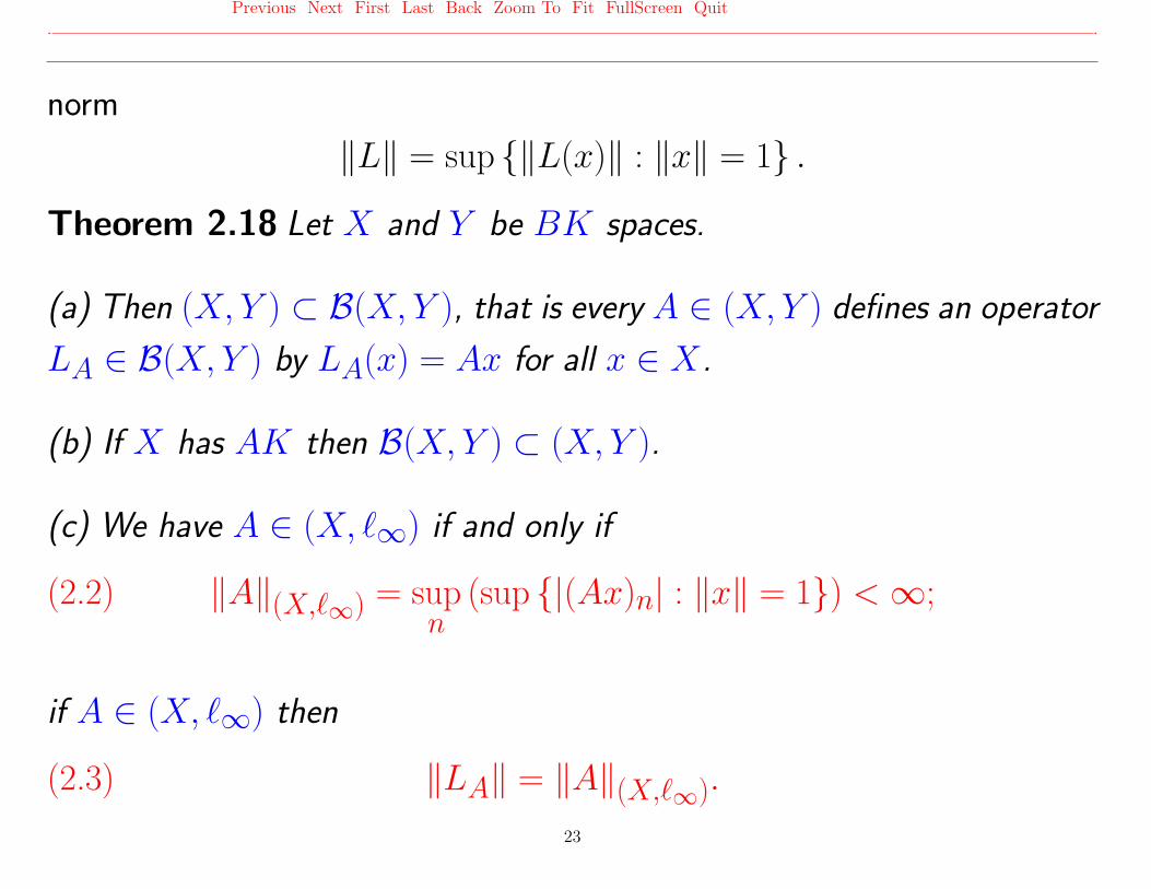
‖L‖ = sup {‖L(x)‖ : ‖x‖ = 1} .

Theorem 2.18 Let X and Y be BK spaces.

(a) Then (X, Y ) ⊂ B(X, Y ), that is every A ∈ (X, Y ) defines an operator

LA ∈ B(X, Y ) by LA(x) = Ax for all x ∈ X.

(b) If X has AK then B(X, Y ) ⊂ (X, Y ).

(c) We have A ∈ (X, `∞) if and only if

(2.2) ‖A‖(X,`∞) = supn

(sup {|(Ax)n| : ‖x‖ = 1}) < ∞;

if A ∈ (X, `∞) then

(2.3) ‖LA‖ = ‖A‖(X,`∞).

23


Proof. (a) This is Theorem 2.8.

(b) Let L ∈ B(X, Y ) be given.

We write Ln = Pn ◦ L for all n, and put ank = Ln(e(k)) for all n and k.

Let x = (xk)∞k=0 ∈ X be given.

Since X has AK, x =∑∞

k=0xke(k), and since Y is a BK space, Ln ∈ X∗

for all n. Hence

Ln(x) =

∞∑k=0

xkLn(e(k)) =

∞∑k=0

ankxk = (Ax)n for all n,

and so L(x) = Ax.

(c) The sufficiency of (2.2) is trivial.

Assume A ∈ (X, Y ).

24


Then LA ∈ B(X, `∞) by Part (a), hence

‖LA(x)‖∞ ≤ ‖LA‖ for all x ∈ X,

and (2.2) is an immediate consequence.

Also, (2.3) is obvious from the definitions of the operator norm and the

norm ‖ · ‖(X,`∞). �

25


3. Multiplier and Dual Spaces

The so–called β–duals are of importance in the theory of matrix transfor-

mations. They are special cases of the multiplier spaces. Let cs and bs be

the sets of all convergent and bounded series.

Definition 3.1 Let X and Y be subsets of ω. Then

M(X, Y ) ={a ∈ ω : ax = (akxk)∞k=0 ∈ Y for all x ∈ X

}is called the multipler space of X in Y. Special cases are

Xα = M(X, `1), the α– dual of X,

Xβ = M(X, cs), the β– dual of X,

Xγ = M(X, bs), the γ– dual of X.

26


Proposition 3.2 Let X, X1, Y , Y1 ⊂ ω and {Xδ} be a collection of

subsets of ω. Then

(i) Y ⊂ Y1 implies M(X, Y ) ⊂ M(X, Y1)

(ii) X ⊂ X1 implies M(X1, Y ) ⊂ M(X, Y )

(iii) X ⊂ M(M(X, Y ), Y )

(iv) M(X, Y ) = M (M(M(X, Y ), Y ), Y )

(v) M

(⋃δ

Xδ, Y

)=⋂δ

M(Xδ, Y ).

Definition 3.3 Let X ⊃ φ be an FK space and X ′ be the continuous

dual of X. Then Xf = {(f (e(n)))∞n=0 : f ∈ X ′} is called the functional

dual of X.

27


Theorem 3.4 (a) Let † denote any of the symbols α, β and γ. Then

Xα ⊂ Xβ ⊂ Xγ ⊂ Xf and X ⊂ X††.

(b) Let X ⊃ φ be an FK space. Then

Xf = (clX(φ))f .

(c) If X ⊂ Y then Xf ⊃ Y f . If X is closed in Y then Xf = Y f .

Example 3.5 Let X = c0⊕z with z unbounded. Then X is a BK space,

Xf = `1 and Xff = `∞, so X 6⊂ Xff .

Theorem 3.6 Let X ⊃ φ be an FK space.

(a) If X has AK then Xβ = Xf .

(b) If X has AD then Xβ = Xγ.28


Theorem 3.7 Let X ⊃ φ be an FK space. Then Xβ ⊂ X ′; this means,

that there is a linear one–to–one map T : Xβ → X ′. If X has AK then

T is onto.

The map T of Theorem 3.7 is defined as follows

T :Xβ → X ′

a 7→ fa ∈ X ′ where fa =

∞∑k=0

akxk for all x ∈ X.

Theorem 3.8 Let X ⊃ φ be an FK space. Then Xf = X ′ if and only

if X has AD.

29


The following results do not extend to FK spaces, in general.

Theorem 3.9 Let X ⊃ φ and Y be BK spaces. Then Z = M(X, Y ) is

a BK space with

‖z‖ = sup{‖xz‖ : ‖x‖ ≤ 1} for z ∈ Z.

Theorem 3.10 Let X ⊃ φ be a BK space. Then Xf is a BK space.

Theorem 3.11 Let X ⊃ φ be a BK space. Then

Xff ⊃ clX(φ).

Hence, if X has AD, then X ⊂ Xff .

30


Example 3.12 (i) M(c0, c) = `∞; (ii) M(c, c) = c; (iii) M(`∞, c) = c0.

Example 3.13 Let † denote any of the symbols α, β or γ. Then

ω† = φ; φ† = ω; c†0 = c† = `

†∞ = `1

`†1 = `∞; `

†p = `q (1 < p < ∞; q = p/(p− 1)).

Example 3.14 We have cβ = cf = `1. The map T of Theorem 3.7 is

not onto. We consider lim ∈ X ′. If there were a ∈ Xf with lim a =∑∞k=0akxk then it would follow that ak = lim e(k) = 0, hence lim x = 0

for all x ∈ c, contradicting lim e = 1.

Example 3.15 Let X = c0 ⊕ z with z ∈ `∞. Then

Xff = `f1 = `∞ ⊃ X,

but X does not have AD, hence the condition of Theorem 3.10 is not

necessary.

31


4. Matrix Transformations

We apply the results of the previous sections to give necessary and sufficient

conditions on the entries of a matrix A to be in a class (X,Y).

The first two results concern the transpose AT of a matrix A.

Theorem 4.1 Let X be an FK space and Y be any set of sequences.

If A ∈ (X, Y ) then AT ∈ (Y β, Xf ).

If X and Y are BK spaces and Y β has AD then

AT ∈ (Y β, clXf (Xβ)).

Theorem 4.2 Let X and Z be BK spaces with AK and Y = Zβ.

Then (X, Y ) = (Xββ, Y ); furthermore

A ∈ (X, Y ) if and only if AT ∈ (Z,Xβ).

32


Remark 4.3 The results of the previous sections yield the characterisations

of the classes (X, Y ) where X and Y are any of the spaces `p (1 ≤p ≤ ∞), c0, c with the exceptions of (`p, `r) where both p,r 6= 1,∞(the characterisations are unknown), and of (`∞, c) (Schur’s theorem 1.2)

and (`∞, c0) ([S–T, 21 (21.1)] (no functional analytic proof seems to be

known).

The class (`2, `2) was characterised by Crone ([Cro] or [Ruc, pp. 111–115]).

Example 4.4 (a) We have (c0, `∞) = (c, `∞) = (`∞, `∞); furthermore

A ∈ (`∞, `∞) if and only if

(4.1) ‖A‖(∞,∞) = supn

∞∑k=0

|ank| < ∞.

If A is in any of the classes above then

‖LA‖ = ‖A‖(∞,∞).

33


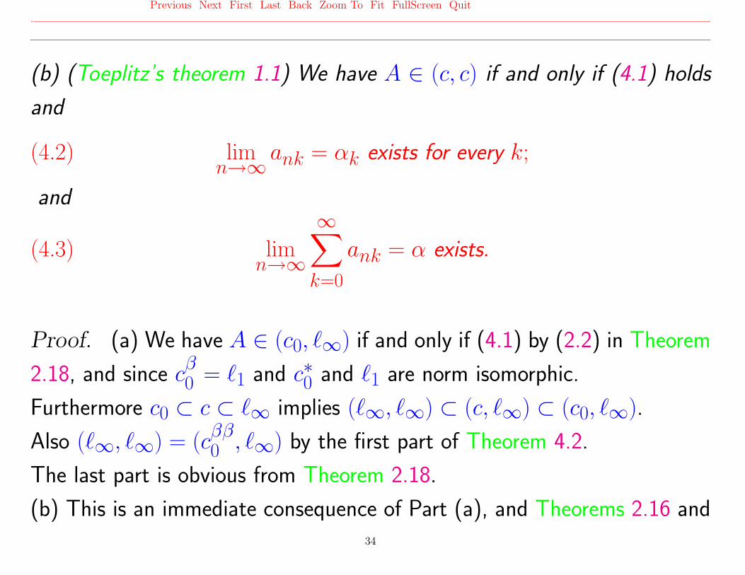
(b) (Toeplitz’s theorem 1.1) We have A ∈ (c, c) if and only if (4.1) holds

and

(4.2) limn→∞

ank = αk exists for every k;

and

(4.3) limn→∞

∞∑k=0

ank = α exists.

Proof. (a) We have A ∈ (c0, `∞) if and only if (4.1) by (2.2) in Theorem

2.18, and since cβ0 = `1 and c∗0 and `1 are norm isomorphic.

Furthermore c0 ⊂ c ⊂ `∞ implies (`∞, `∞) ⊂ (c, `∞) ⊂ (c0, `∞).

Also (`∞, `∞) = (cββ0 , `∞) by the first part of Theorem 4.2.

The last part is obvious from Theorem 2.18.

(b) This is an immediate consequence of Part (a), and Theorems 2.16 and34


2.17. �

Example 4.5 We have (`1, `1) = B(`1, `1) and A ∈ (`1, `1) if and only if

(4.4) ‖A‖(1,1) = supk

∞∑n=0

|ank| < ∞.

If A ∈ (`1, `1) then

(4.5) ‖LA‖ = ‖A‖(`1,`1).

Proof. Since `1 has AK, Theorem 2.18 (b) yields the first part.

We apply the second part of Theorem 4.2 with X = `1, Z = c0, BK

spaces with AK, and Y = Zβ = `1 to obtain A ∈ (`1, `1) if and only if

AT ∈ (`∞, `∞); by Example 4.4 (a), this is the case if and only if (4.4) is

35


satisfied.

Furthermore, if A ∈ (`1, `1) then

‖LA(x)‖1 =

∞∑n=0

∣∣∣∣∣∣∞∑

k=0

ankxk

∣∣∣∣∣∣ ≤∞∑

k=0

∞∑n=0

|ankxk| ≤ ‖A‖(1,1)‖x‖1

implies

‖LA‖ ≤ ‖A‖(1,1).

Also have LA ∈ B(`1, `1) implies

‖LA(x)‖1 = ‖Ax‖1 ≤ ‖LA‖ ‖x‖1,

and it follows from ‖e(k)‖1 = 1 for all k that

‖A‖(1,1) = supk

∞∑n=0

|ank| = supk‖LA(e(k))‖1 ≤ ‖LA‖.

�

36


5. Measures of Noncompactness

Now we find necessary and sufficient conditions for a matrix A ∈ (X, Y )

to define a compact operator LA.

This can be achieved by applying the Hausdorff measure of noncompact-

ness.

The first measure of noncompactness was defined and studied by Kura-

towski ([Kur]), and later used by Darbo ([Dar]).

The Hausdorff measure of noncompactness was introduced and studied by

Goldenstein, Gohberg and Markus ([GGM]).

Istratesku introduced and studied the Istratesku measure of noncompact-

ness ([Ist]).

The interested reader is referred for measures on noncompactness to [AKP,

B–G, Ist1, TBA, M–R].

37


We will only consider the Hausdorff measure of noncompactness; it is the

most suitable one for our purposes.

Let (X, d) be a metric space, x0 ∈ X and r > 0. Then

B(x0, r) = {x ∈ X : d(x, x0) < r}

denotes the open ball of radius r, centred at x0.

Definition 5.1 Let (X, d) be a metric space and M denote the collection

of bounded subsets of X. The function χ : M→ [0,∞) with

χ(Q) =

ε > 0 : Q ⊂n⋃

k=0

B(xk, rk); xk ∈ X, rk < ε

is called Hausdorff measure of noncompactness; χ(Q) is called

the Hausdorff measure of noncompactness of Q.

38


Proposition 5.2 Let X be a metric space and Q,Q1,Q2 ∈M. Then

χ(Q) = 0 if and only if Q is totally bounded,

χ(Q) = χ(Q),

Q1 ⊂ Q2 implies χ(Q1) ≤ χ(Q2),

χ(Q1 ∪Q2) = max{χ(Q1), χ(Q2)},χ(Q1 ∩Q2) ≤ min{χ(Q1), χ(Q2)}.

Proposition 5.3 Let X be a normed space and Q,Q1,Q2 ∈M. Then

χ(Q1 + Q2) ≤ χ(Q1) + χ(Q2),

χ(Q + x) = χ(Q) for all x ∈ X,

χ(λQ) = |λ|χ(Q) for all scalars,

χ(Q) = χ(conv(Q)).

39


Theorem 5.4 (Goldenstein, Gohberg,Markus) ([GGM])

Let X be a Banach space with a Schauder basis (bk)∞k=0, Q ∈ M and

Pn : X → X be the projector onto the linear span of {b0, b1, . . . , bn}.Then

(5.1)1

alim supn→∞

(supx∈Q

‖(I − Pn)(x)‖

)≤ χ(Q) ≤

≤ lim supn→∞

(supx∈Q

‖(I − Pn)(x)‖

)where

a = lim supn→∞

‖I − Pn‖.

So far we considered the measure of noncompactness of bounded subsets

of a metric space. Now we define the measure of noncompactness of an

operator.40


Definition 5.5 Let κ1 and κ2 be measures of noncompactness on the

Banach spaces X and Y , and MX and MY denote the collections of

bounded sets in X and Y . An operator L : X → Y is said to be (κ1, κ2)–

bounded if

L(Q) ∈MY for all Q ∈MX

and there exists a non–negative real c such that

κ2(L(Q)) ≤ c κ1(Q) for all Q ∈MX .

If an operator L is (κ1, κ2)–bounded, then the number

‖L‖(κ1,κ2)= inf{c ≥ 0 : κ2(L(Q)) ≤ c κ1(Q) for all Q ∈MX}

is called the (κ1, κ2)–mesaure of noncompactness of L.

If κ = κ1 = κ2, then we write ‖L‖κ = ‖L‖(κ,κ).

41


Theorem 5.6 Let X and Y be Banach spaces, L ∈ B(X, Y ), SX and

BX be the unit sphere and the closed unit ball in X, and χ be the Hausdorff

measure of noncompactness.

Then

(5.2) ‖L‖χ = χ(L(SX)) = χ(L(BX)).

Theorem 5.7 Let X, Y and Z be Banach spaces, L ∈ B(X, Y ), L ∈B(Y, Z), and C(X, Y ) denote the set of compact operators in B(X, Y ).

Then ‖ · ‖χ is a seminorm on B(X, Y ) and

‖L‖χ= 0 if and only if L ∈ C(X, Y ),(5.3)

‖L‖χ ≤ ‖L‖,‖L ◦ L‖χ ≤ ‖L‖χ ‖L‖χ.

42


Theorem 5.8 Let L ∈ B(`1, `1), and A denote the infinite matrix such

that L(x) = Ax for all x ∈ `1. Then L ∈ C(`1, `1) if and only if

(5.4) limr→∞

(supk

∞∑n=r

|ank|

)= 0.

Proof. By Theorem 2.18 (b), every L ∈ B(X, Y ) can be represented by

a matrix A ∈ (X, Y ).

Writing S = S`1, we have by (5.2) in Theorem 5.6

‖L‖χ = χ(L(S)).

For r = 0, 1, . . . , let A(r) be the matrix with the first r rows replaced by

0. Then

‖(I − Pr−1)(L(x))‖1 = ‖A(r)x‖1

43


hence, by (4.4) in Example 4.5,

supx∈S

‖(I − Pr−1)(L(x))‖1 = ‖A(r)‖(`1,`1)= sup

k

∞∑n=r

|ank|.

Since obviously ‖I − Pr−1‖ = 1 for all r, and the limit on the right hand

side of (5.4) exists, it follows from (5.1) in Theorem 5.4 that

χ(L(S)) = limr→∞

(supk

∞∑n=r

|ank|

).

Finally it follows from (5.3) in Theorem 5.7 that L ∈ C(X, Y ) if and only

if (5.4) is satisfied. �

Remark 5.9 It follows from Theorem 5.8 and Example 4.5 that every L ∈B(X, Y ) is compact.

44

REFERENCES


REFERENCES

References

[AKP] R. R. Akhmerov, M. I. Kamenskii, A. S. Potapov, B. N. Sadovskii, Measures of Noncompactness

and Condensing Operators, Operator Theory: Advances and Applications, Vol. 55, Birkhauser, Basel,

1992 37

[B–G] J. Banas, K. Goebel, Measures of Noncompactness in Banach Spaces, Lecture Notes in Pure and

Applied Mathematics, Vol. 60, Marcel Dekker, New York, 1980 37

[Cro] L. Crone, A characterization of matrix mappings on `2, Math. Z. 123 (1971), 315–317 33

[Dar] G. Darbo, Punti uniti in transformazioni a condominio non compatto, Rend. Sem. Math. Univ.

Padova 24 (1955), 84–92 37

[GGM] I. T. Gohberg, L. S. Goldenstein, A. S. Markus, Investigations of some properties with their q–norms,

Ucen. Zap. Kishinevsk. Univ. 29 (1957), 29–36 (Russian) 37, 40

[Har] G. H. Hardy, Divergent Series, Oxford University Press, 1973 4

[Ist] V. Istratesku, On a measure of noncompactness, Bull. Math. Soc. Sci. Math. R. S. Roumanie

(N.S.) 16 (1972), 195–197 37

[Ist1] V. Istratesku, Fixed Point Theory, An Introduction, Reidel, Dordrecht, Boston and London, 1981

37

45

REFERENCES


REFERENCES

[K–G] P. K. Kamthan, M. Gupta, Sequence Spaces and Series, Marcel Dekker, New York, 1981 10

[Kur] K. Kuratowski, Sur les espaces complets, Fund. Math 15 (1930), 301–309 37

[Mad] I. J. Maddox, Elements of Functional Analysis, Cambridge University Press, 1971 4, 9

[Mad1] I. J. Maddox, Infinite Matrices of Operators, Lecture Notes in Mathematics 780, Springer Verlag,

Heidelberg–Berlin–New York, 1980 9

[M–R] E. Malkowsky, V. Rakocevic, An introduction into the theory of sequence spaces and measures of

noncompactness, Zbornik radova, Matematicki institut SANU 9(17) (2000), 143–234 9, 10, 37

[Pey] A. Peyerimhoff, Lectures on Summability, Lecture Notes in Mathematics 107, Springer Verlag,

Heidelberg–Berlin–New York, 1969 4

[Ruc] W. H. Ruckle, Sequence Spaces, Research Notes in Mathematics 49, Pitman, Boston, London,

Melbourne, 1981 33

[S–T] M. Stieglitz, H. Tietz, Matrixtransformationen in Folgenraumen, Math. Z. 154 (1977), 1–16 9, 33

[Toe] O. Toeplitz, Uber allgemeine Mittelbildungen, Prace. Mat. Fiz. 22 (1911), 113–119 6

[TBA] J. M. Ayerbe Toledano, T. Dominguez Benavides, G. Lopez Acedo Measures of Noncompactness

in Metric Fixed Point Theory, Operator Theory, Advances and Applications, Vol. 99, Birkhauser,

Basel, Boston, Berlin, 1997 37

46

REFERENCES


REFERENCES

[Wil1] A. Wilansky, Functional Analysis, Blaisdell Publishing Company, New York, Toronto, London, 1964

10

[Wil2] A. Wilansky, Summability through Functional Analysis, North–Holland Mathematical Studies 85,

Elsevier Science Publishers, Amsterdam, New York, Oxford, 1984 9, 10, 20

[Zel] K. Zeller, Abschnittskonvergenz in FK–Raumen, Math. Z. 55 (1951), 55–70 10

[Z–B] K. Zeller, W. Beekmann, Theorie der Limitierungsverfahren, Springer Verlag, Heidelberg–Berlin–

New York, 1968 4, 9

47

Documents

Modern Functional Analysis in the Theory of Sequence ...tesla.pmf.ni.ac.rs/matematika/malkowsky/talkfk.pdf · Modern Functional Analysis in the Theory of Sequence Spaces and Matrix