MODERN EPIDEMIOLOGY - McGill University · MODERN EPIDEMIOLOGY Professor, Department of Family and Community Medicine, University of Massachusetts Medical School, Worcester, Massachusetts

MODERN EPIDEMIOLOGY

Professor, Department of Family and Community Medicine, University of Massachusetts Medical School, Worcester, Massachusetts

LITTLE, BROWN AND COMPANY BostonlToronto

CONTENTS

Preface xi Acknowledgments m

1. THE EMERGENCE OF EPIDEMIOLOGY

2. CAUSAL INFERENCE IN EPIDEMIOLOGY Philosophy of Scientific Inference 7 A General Model of Causation 10 Causal Infuence in Epidemiology 1 G

3. MEASURES OF DISEASE FREQUENCY Incidence 23 Cumulative Incidence 29 Preualence 32

4. MEASURES OF EFFECT Absolute Effect 35 Relative Effect 36 Anributable Proportion 38

5. STANDARDIZATION OF RATES Tbe Principle of Standardization 41 'Ilndirect" V m 'Direct" Standardization 45

6. TYPES OF EPIDEMIOLOGIC STUDY Experimental Studies 52 None%perimental Studies 55

7. OBJECTIVES OF EPIDEMIOLOGIC STUDY DESIGN Precision ( h c k of Random Error) 78 Validity ( h c k of Systematic Error) 82

8. STRATEGIES INTHE DESIGN OF EPIDEMIOLOGIC STUDIES Improving Precision 99 Improving Validity 102

9. THE ROLE OF STATISTICS IN EPIDEMIOLOGIC ANALYSIS A s s m t of Random Variability 115 Tbe Assesnnent and Control of Confounding 125

10. FUNDAMENTALS OF EPIDEMIOLOGIC DATA ANALYSIS Data Editing 131 Data Reduction U4 Effect Estimution (and Hypothesis Testing) UG

CONTENTS

1 1. ANALYSIS OF CRUDE DATA Hypothesis Testing with Crude Data 153 Estimation of Effects with Crude Data 164

1 2. STRATIFIED ANALYSIS ' 177 Eualudtion and Control of Confounding 178

POINT ESTIMATION.OF A UNIFORM EFFECT ,181

Pooling with Inverse variances (Direct Pooling) 183 Pooling Using thy Method of Maximum Likelihood 190 Pooling with Mantel-Haenszel I Estimators 195 , , STATISTICAL HYPOTHESIS TESTING FOR STRATIFIED DATA 197

Hypothesis Testing with Stratified Person-Time Data 198 Hypothesis Testing with Stratified Cumulauve Incidence, Prevalence, or Case-Control Data (2 x 2 Tables)'203

CONFIDENCE LNTERVALS FOR FOOLED ESTIMATES OF EFFECT 208 ~ Confidence Inrervals for Stratified Person-Time Data 208 Confidence Inrervals for Stratified Cumulative Incidence Dara 214 Confidence 1 n r e d s for the Odds Ratio from Stratified Case-Control (or Prevalence) Dara 217

EVALUATION OF EFFECT'MODIFICATION ,221 I DESCRIPTION OF EFFECT MODIFICATION 226 Standardized Effect Estimates 227 Effect Functions 233

13. MATCHING . Princzples of Matching 23 7

OVERMATCHING 247 . MATCHING ON INDICATORS OF INFORMATION QUALITY 249

Matched Case-Contml Analysis 250 I POINT ESTIMATION OF THE RELATIVE RISK (ODDS RATIO) FROM MATCHED

GASE-CONTROL DATA 251 STATISTICAL ~ o T H E S I S TESTING WITH MATCHED CASE-CONTROL

DATA 258 INTERVAL ?STIMATJON OF THE ODDS RATIO WITH MATCHED CASE-CONTROL

DATA 4

Matched ~ o i l h ~ - u ~ Studies 275 . '

Evalmtion 0fEfect Modzf?uition with Matched Data 279 Evalation of the E$ct of Matching with Case-Control Data 280 Multivariate ~rhlysis of Matched Data 281 .

14. MULTIVARIATE ANALYSIS Basic Mathematical Modek 286 Designing Multivariate Modehi for Inference 299 Multivariate Modek in Ecologic Analysis 304 Shengths and Limitations of Multivariate Modehi 306 Use of a Confounder Summa y Score 307

15. INTERACI'IONS BETWEEN CAUSES Defining Interaction 313 Measuring Interaction 320

16. ANALYSIS WITH MULTIPLE LEVELS OF EXPOSURE Estimation of Efects for Multipe Leuek of Exposure 332 Statktical Hypothesis Testng for Trend 346 Multivariate Analysis of Trend 348

PREFACE

The tenets of epidemiology, like those of every other science, have become established piecemeal. Some are more useful than others, and some exist in mutual conflict. In this book my aim has been to weave the diverse threads of epidemiologic concepts and research methods into a single fabric. I have tried to reconcile conflicting ideas and unlfy the conceptual foundation, omitting needless partitions. In particular, I have labored to tie the statistical topics of epidemiologic analysiswhich have a way of generating their own special goals, momentum, and ling-to the basic goals of epidemiologic research I have also ventured to reconcile epidemiologic principles with the broader goals and methods of scientific in- quiry, as I understand them. In sewing the final cloth, I have been mindful that I cannot succeed fully, but rather must fail in my attempts to varying degrees. Intent readers will surely find holes in the fabric and an incorrect stitch here and there. Some of these irregularities undoubtedly reflect in- adequate understanding or communication on my part Some mark conceptual areas, such as confounding and interaction between causes, where development is progressing rapidly. I hope that such problems are few, and small enough not to impair the overall usefulness of the work.

Throughout this book I have strived to make the material accessible to a novice to the field. Whenever possible the descriptions are verbal rather than mathematical, despite the quantitative objectives of research The first

I

I eight chapters deal with fundamental issues of epidemiologic conceptual-

I ization, measurement, and study design, and should be comprehensible I even to those who lack previous trainlng in epidemiology or statistics; the

second eight chapters address the somewhat more technical issues of epidemiologic data analysis, but even these topics are presented with step

1 by step explanations and simplicity as a central objective. Chapters 1 through 5 form an introductory unit on basic epidemiologic

concepts and tools. Chapter 1 places epidemiology in its historical per-

: spective. Chapter 2 ventures into the philosophic foundation for epidemiology, providing a model for causal action that serves as a platform for understanding etiology and its quantitative description. Chapters 3 through 5 continue with the fundamental measures of epidemiology (incidence, prevalence, and risk) and the measures derived from them to quantify causal actions.

Chapters G through 8 form a second unit that deals with epidemiologic studies. The basic types of studies are presented in Chapter 6, where I have pursued steadfastly the objective of a unified approach, stressing the theoretical connections among study types. Chapters 7 and 8 explore the issues of study design without resorting to mathematical notation. They emphasize the sources of error in effect estimates as well as the quantitative nature of most aspects of study design.

Chapters 9 through 16 deal with data analysis. In this section some re- liance on mathematical formulations has been unavoidable, and I have assumed a basic knowledge of the relevant statistical distributions. Never-

xii PREFACE xiii

theless, the fundamental statistical priil>iples are introduced and explained in Chapters 9 and 10 using as little notation as possible. Chapter 11 intro- duces the basic .arialjrtic formulations for crude data, which are extended. iil Chaprers 12 and 13 for stratified and matched data. Chapters 11 through 13 cover the routine analytic tasks that.an epidemiologist faces; consequently, these are the most technical chapters in the book. Various ap- proqches are described in derail, so that these chapters can be used as a reference for febearchas, as well as an insrructional guide to the fundamental analytic- methods.

~he'final three ~habters turn t6 more advanced analytic topics, but the emphasis is not so much on formulas is on analytic strategies. Thus, Chap- ter 14 on mu!tivariate analysis is probably the least technical description of ingltivariate analysis in any &book; it provides practical guidance on choosing, coristfucting, and interpreEing rilultivariate models. Chapters 15 md 1.6 deal yith the.advanced topics of interaction and "dose-response" evduiitim, but, the emphasis once again is on the principles and pitfalls of such kalyses, .rather .than onxhe technical aspects of the requisite calcu- l2tions. I could not avoid formulas entirely and still provide an adequate discussion of these topics, but the formulas presented illustrate approaches of conceptual simplicity amenable to a pencil-and-paper solu- ri-on. I

In my effora'td tie together epidemidogic concepts for all these topics, I have encountered some fossilized divisions that I consider no longer 1 useful. Fo-r example, a rift has separated the traditional area of infectious I disese epidemiology from the more recent and growing area of "chronic" ! i disease. epidemiology. I have never been persuaded of any rationale for 1 this,;distinct:ion:The terms "infectious" and "chronic" are neither mutually j exclusive i ~ o r collectively exhaustive ,alternatives. Many diseases are both infectious and some, such as fatal traumatic injury, are neither. '"Ghroriic" h s so~et imes been take'n to mean a long induction period, rather thm P long period of manifestation, but this redefinition still fails €0 ~ a k e a .heeani&ful distinction, between C ~ O conceptually different types of .epidkmiol&y ,Although some specialized methods have been 'devel-

eitf5t between traditional and modern areas of epidemiology are certainly aped solely t'o s h d i the spread df ~nfectious illness, whatever distinctions

less i-mmportant'than the broad base of concepts that are shared. This book does not dealwith models for epidemic spread, but focuses on the general epidemio1ogic. co'n;epts that apply to all diseases, infectious or not, chronic or'not;.and 50 causes that have short or long induction periods.

Another distinction that has been used to categorize epidemiologic w&k is its classification into 'descriptive and analytic epidemiology. My viqv isthat this demarcati0n.k also best forgotten. It has been used in fefet-ehce both to specific studyvhiables (so-called "descriptive" variables beiiig distinguished from putative causes) and to entire studies, but in fieither context'doei it hold as a sensible classification scheme. No quali-

tative distinction, other than a completely arbitrary one, distinguishes "descriptive" variables from more fundamental risk factors. Any disease de- terminant can be specified in terms of more proximal determinants or previously unsuspected confounding factors. The division of epidemiologic research into descriptive and analytic compartments has given rise to the illusion that there are diierent sets of research principles that apply to descriptive and analytic studies. This notion devolves from a mechanical view of scientific research, and diverges from prevailing doctrines of scientific philosophy. For example, the view that "descriptive data" from "exploratory studies" generate hypotheses, whereas the data from "analytic studies" are used to test hypotheses, does not cohere with a broader understanding of science. Hypotheses are not generated by data; they are proposed by scientists. The process by which scientists use their irnagi- nation to create hypotheses has no formal methodology and is certainly not prescriptive. Any study, whether considered exploratory or not, can serve to refute a hypothesis. It is not useful to regard some studies merely as "hypothesis generating" and others as "hypothesis testing," because the inexorable advance of scientific knowlege cannot be constrained by such rigidities.

I believe that epidemiology is much more coherent than these traditional divisions would suggest. Even the stark contr.ast between follow-up studies and case-control studies has been softened as understanding of the basic principles of epidemiology has progressed. In writing this book, my greatest hope is to convey to the reader the conviction that epidemiologic principles can be understood as an integrated substrate of logical ideas, rather than as a jumble of isolated and sometimes conflicting postulates.

K. J. R.

10. FUNDAMENTALS OF EPIDEMIOLOGIC DATA ANALYSIS

In a well-planned study, the raw observations that constitute the data contain the information that satisfies the objectives of the study. In Chapter 7 it was emphasized that a study is a measurement exercise and that the overall goal for a study is accuracy in measurement. Accordingly, the goal in data analysis is to extract the pertinent measurement information from the raw observations.

Typically, there are several distinct stages in the analysis of data. In the preliminary stage, the investigator should review the recorded data for accuracy, consistency, and completeness; this process is often referred to as data editing. Next, the investigator should summarize or transform the data into a concise form for subsequent analysis, usually into contingency tables that tabulate the distribution of the observations according to key factors; this stage of the analysis is referred to as data reduction. Finally, the edited and reduced data are used to generate the epidemiologic measures of interest, typically one or more measures of effect (such as relative risk estimates), with appropriate confidence intervals. This last stage of analysis is sometimes considered the analysis proper, but it is more convenient to refer to it as effect estimation (or perhaps just estimation, if the goal of the analysis is to estimate disease frequency rather than to measure an effect). For some investigators, the last stage of analysis inevitably in- cludes statistical hypothesis testing. The previous chapter explained why hypothesis testing is an undesirable feature of data analysis in most epidemiologic situations. Since the statistical theory behind interval estimation is closely related to statistical hypothesis testing, however, it is useful to consider the issues described in statistical hypothesis testing as a foun- , dation for understanding epidemiologic data analysis.

DATA EDITING There is no excuse for failing to scrutinize the raw data intensely for errors and to correct such errors whenever possible. Errors are routinely introduced into data in a variety of ways; some errors are detectable in editing and some are not.

The data in an epidemiologic study usually derive from a self-adrninis- tered or an interviewer-administered questionnaire or from existing rec- ords that are transcribed for research. The data from the questionnaire or record-abstraction form may be transcribed from this primary form to a code form for machine entry, usually by keypunching. Coding of re- sponses is often necessary. For example, occupational data obtained from interviews need to be classified into a manageable code, as does drug information, medical history, and many other types of data. Data such as age or year of birth (year of birth is usually preferable to age, since it tends to be reported more accurately and does not change with time), although

oftei grouped:i.*to broad categories for reporting purposes, should be recorded in a precise.form rather than grouped because the actual values will ',allow greater 'flexibility later in the analysis: For example, different groupings may be necessary for compnisons with several other studies. Some nominal scale variables that have only a few possible values can be -precbded on the primary forms' by checking a designated box corresponding to the appcopriate category. For .nominal scale variables with many .possible categories; .however, such as country of birth or occupation, pre- co-ged questions are not practical. If all data items can be precoded, it may be f e ~ i b l e to collect the data in ,a primary form that can be read directly by a machine, hy optical scanning, or,by some comparable method. Oth- emise, it will' us6ally be necessary to trawlate the information on the pfimry data fqrm before it is stored in a machine or in machine-readable fo-r-m.

It is p0.ssibl.e ~d .usua l ly desirable to avoid rewriting the data onto a secodary data form during the coding pprocess. Rather than generating addifi.orral fraimiiption errors, it is preferable to code the data while si- multaiieously keyings them into a computer storage system. A computer pc@rarii can be ,devised to prompt data entry item by item, displaying category codes on a terminal. screen to assist in coding. If the data are coded $d mtircen by hand, they will often require keypunching anyway, unless they'are coded onto optical scanning sheets; consequently, direct &G,'eritry duririg 'coding reduces,both costs and errors. The fewer the number- of rewriting 'operations between the primary record and the machine-=stored version,, the fewer.the.errors that are likely to occur. If rewriting is unavoidable, it is useful to assess the extent of coding errors in the'f-i~e'n form by coding a pr6portion of the data forms twice, inde- pendently. Tlie.information thus obtained can be used to judge the mag- ri-it.u& of bias introduced by misclassification from coding errors.

Basic editing of ,the data involves checking each variable for illegal or uhusuil values. For example, gender may be coded 1 for male and 2 for fmake. Usually 'a separate value, perhaps 3, is used to designate an unknown,value. It is preferable not to assign a code of zero if it can be avoided because:mi$sing information or non-numeric codes may be interpreted by somemachines or programs as a zero. By not assigning zero as a specific code, nQt wen for unknown information, it may be possible to detect .keyp\iriching 'errors or missing information. The distribution of e ~ h vafiiible should be exmined in the editing process. Any inadmissible values should be checked against the primary data forms. Unusual values Such as unknown gender or unusual age or birth year should also be checked

In addition to checking for incorrect or unusual values, the distribution of each variable'should be examined to see if it appears reasonable. Would you expect about half of the subjects to be males, about 80 percent (a reasonable figure if the subjects have, say, upper respiratory cancer), or

FUNDAMENTALS OF EPIDEMIOLOGIC DATA ANALYSIS 133

about 2 percent (if the subjects are nurses)? Such an evaluation may reveal important problems that might not otherwise come to light. For example, a programming error could shlft all the data in each electronic record by one or more characters, thereby producing gibberish that nevertheless might not be detectable in, say, a multivariate analysis (an important drawback of the multivariate approach). The potential for such a disaster heightens the need to check carefully the distribution of each variable during the editing of the data

The ediung checks described so far relate to each variable in the data taken singly. In addition to such basic editing, it is usually desirable to check the consistency of codes for related variables. It is not impossible, but it is improbable that a person 18 years of age will have three children Males should not have been hospitalized for hysterectomy People over 2 meters tall are unlikely to weigh less than 50 kilograms. Thorough editing will involve many such consistency checks and is best accomplished by computer programs designed to flag such errors [MacLaughlin, 19801. Oc- casionally an apparently inconsistent result may appear on checking to be correct, but many errors will turn up through such editing. It is importanr, also, to check the consistency of various distributions. If exactly 84 women in a study are coded as premenopausal for a variable, "type of menopause," then it is reassuring that exactly 84 are likewise coded as premenopausal for the variable "age at menopause" (for such a variable, the code "premenopausal" should take a different code number from that assigned to unknown-e.g., 98 for premenopausal and 99 for unknown).

An important advantage of coding and enterlng data through a computer program is the ability to edit the data automatically during the entry process. Inadmissible or unusual values can be screened as they are entered. Inadmissible values can be rejected and corrected on the spot by programming the machine to print an error message on the screen and give an audible message as well to alert the operator about the error. Unlikely but legal values can be brought to the operator's attention in the same way. A sophisticated data-entry program can also check for consistency between variables and can eliminate some potential inconsistencies by automatically supplying appropriate codes. For example, if a subject is premenopausal, the program can automatically supply the correct code for "age at menopause" and skip the question. (On the other hand, some investigators may prefer the redundancy of the second question to guard against an error in the first.)

Even with sophisticated editing during data entry, it is still important to edit the stored data before analysis, to check on the completeness of the data and the reasonableness of the distribution of each variable. Neither of these features can be evaluated by a data-entry program.

Every experienced investigator knows that even the most meticulous data collection efforts sufFer from errors that are detectable during careful editing. If editing is planned as a routine part of handling the data, the

existence of such errors is usually not a serious problem. If editing is ignored, momentous problems can result.

DATA %DUCTION ,

The mtion fufunclarilental to data reduction is that certain observations in a set of data are equivalent, and it is easier to deal with equivalent observations %ftei they havelbeen summarized. The summary form usually is a ca;iidrigency.rab-le in which the frequency of subjects (or units of obser- ~~tion) with every specific combination of variable values is tabulated for variabkes of interest. 'such a table is presumed to contain, in summary form, .essentiaily.all, the relevant information in the data. From the contin- gen-q table, the investigator c.an proceed with effect estimation.. In addi- tim, @e, ~ b l e displays the distiibuticsn of subjects according to key variables and thus conveys directly to the investigator an intimacy with the claa t h t is fiat easily obtained &,any 6ther way

D%t:?i r~duction .into a contingehcy table is predicated on an analysis in whi.cti there is no concern for confounding or effect modification or there are at most only .a~small number of variables that might be confounders or effect modfiers. If the analysis must take account of a large number of vziabke5, a multivariate analysis using mathematic modeling will be nec- essay. For such multivariate analyses, it is not necessary to reduce the data into a contirigency table. Nevertheless, to ensure that the investigator ac- quires some f?miliaritjr with the data, it is advisable, even when planning a muktkiriste analysis, ro reduce ihe data into contingency table format for $e variables of central interest. Indeed, proceeding with an abridged mdysSis based on.'thc contingency table data is a good idea even if the n e ~ d f o ~ the rnuioiriiriate analysis is certain.

~oi laps i r i~ die edired data into. categories for the contingency table may i-iecesshte satne.iLecision making: The process is straightforward.for nom- iiial scale variablks such as religion or race, which are already categorized. For cantinuous variables, however, the investigator must decide how many categories to make and where the category boundaries should be. The number i?f categories will usually depend on the amount of data available. If the data are. abundant, it is always preferable to divide a variable into nta~iv'c?tegoi-ies. On the other hand,.the purpose of data reduction is to Summarize tlie data concisely and conveniently; creating too many cate- godes would defeat this purpose. For control of confounding, it is rarely iie'cesSsary to M e &ore than about five categories [Cochran, 19681. If an expcjsure vafiabl? is categorized to examine effect estimates for various level< &f exposure; again it would be unusual to require more than about Five categories.. ~rtqiuentl~, however, the data are so sparse that it is undesirable to create as many as five categories for a given variable. When the observations &e stretched over .too many categories, the numbers


within categories become statistically unstable and produce large random errors in the effect estimates.

Since most of the confounding from a given factor can be removed by a stratified analysis based on only two categories of a continuous variable [Cochran, 19681, it is desirable with sparse data to keep the number of categories small, perhaps two or three. Even a large body of data can be spread too thin if the contingency table involves too many dimensions, that is, if too many variables are used to class* the subjects. With three variables, apart from exposure and disease, and three categories for each variable, there will be 27 2 X 2 tables (assuming that both exposure and disease are dichotomous). With an addirional two variables of three categories each, there will be a total of 243 2 X 2 tables, enough to stretch even a considerable body of data too thin, siince a study of 10,000 people would average only about 10 subjects per cell of the multidimensional table. If a stratified analysis is planned and it is necessary to strat* by several variables, it is probable that only a few, perhaps as few as two, categories can be used for each variable. With only two categories per variable, stratification by five variables requires 32 rather than 243 2 x 2 tables, and a study of 10,000 subjects would average 78 subjects per cell rather than 10, thereby gaining precision at the cost of some potential residual confounding within categories.

The investigator must also decide where to draw the boundary between categories. There is no accepted method for doing this. A frequently expressed concern is that boundaries might be '"gerrymandered," that is, shifted after a preliminary examination of the'effect estimates in such a way that the estimates are altered in a desired direction. This concern imputes a level of dishonesty to the investigator that is presumably uncom- mon. Furthermore, the shift of a boundary in categorization rarely has a substantial effect on the magnitude of an estimate and then only because of a large random error component. On the other hand, it is frequently useful to inspect the distribution of a variable before deciding at which points to carve categories. There may be "natural" categories if the distribution has more than one mode. The distribution may be sufficiently skewed that preconceived category boundaries would lead to an ineffi- cient separation of subjects, with too few in some categories and too many in others. For these reasons, it is often preferable to define the final categories after reviewing the data, notwithstanding the common advice that it is somehow more "objective" to do so in ignorance of the distribution of observations in hand. Nevertheless, if meaningful category boundaries are inherent in the variable, these can and should be specified a priori. For example, in categorizing subjects according to analgesic consumption, it is desirable to create categories that contrast the various therapeutic indications for analgesic use, the recommended doses for which can be specified in advance. It is often desirable, especially for an exposure vari-

. .

able, to retain exrreme. categories in 'the analysis without merging these with neighboring Gtegories, since the extreme categories are often those fiat permit the m ~ s t biologically infotinative contrasts.

A &-unon problem in creating categories is the question of how to deal with .the.erids of the'scale. 0pen:ended categories can provide an oppor- mity for considerable residual confounding, especially if there are no tl-iecsrerical boungs..for the variable. For example, age categories such as 65 + ;with ilo upper limit, allow a considerable r a g e of variability within which 'the desired ho;mogenejQ. of exposure or outcome may not be achieved. Another exapple is the separation of the efects of alcohol consumption, and fobado smoking on the risk of oral cancer; within cate- gdrik~.of heavy smoking, it is a reasonable possibility that the heaviest smqkers drink more aalcohol th& those who smoke less within that cate- g o q .[Rdth-man ind ~el le r , 19721. When residual confounding from open- ended categories is considered likely, strict boundaries should be placed 017. every:catego~,'including those at the extremes of the scale.

A convenient method of assembling.the final categories is to categorize the &fa ini~ial~~mucfimore finely than is necessary A fine categorization will facili6te revi .7 of the distribution for each variable; more usable cat- egoria cm thenbe created by coalescing adjacent categories. The coalescing of adjacent strata for a rankordered confounding variable can be jus- tified byY the, lack of confounding that is introduced by merging the categories.; this merging will not introduce confounding if the exposure diswibotion is +-same among the controls or person-time denominators betw&en t.he stran,lor if the proportion of cases or the disease rate is the same among non,exposed subjects between the strata [Miettinen, 1976bI. The aclvaiitage of starting with more categories than is ultimately necessary is that the merging of categories can be conven~ently accomplished with pencil and paper in seconds or minutes, whereas separating categories i*ro &xi-iceg;ories c@ot be done without reading through the entire data file, thus xdding.&other computer run.

EFFECT E S T ~ ~ T I O N (AND HYPOTHESIS TESTING) Hypothesis .Testing

h data analvsts, is opposed to the broader area of scientific inference, --- ~ , . . - - hypothesis resting generally refers to the evaluation of a null hypothesis. The tntrodwtion of the concepts of statistical evaluation early in the men- -riethcentury ied to an appreciatjonof the importance of assessing the role of r'afidom error in observations. Hypothesis testhg is directed at the ques- ti-on of whether random error might account entirely for an observed as- ..--. .

sockkion. The statist$ used to evaluate this question is the P-value. The P:"alue is usually interpreted as the probability that an association

at k+t . as srrong,as *at actuall? seen in the data might have arisen if the hull hypothesis,were true, that is, by chance alone. Because a low P-value

. ,

FUNDAMENTALS OF EPIDEMIOLOGIC DATA ANALYSIS

r *.' .- V1 Two-tailed P-value c O) = sum of A and B P

.-

0 bbsekad value L . ,. - Effect measure

Fig. 10-1. Distri'bution of effect eshhn26tates under the null hypothesis in large studies (continuous d&tnbution).

indicates a low probability, under the null hypothesis, of results as extreme or more extreme than those observed, low P-values are taken as an indi- cation that the data are more compatible with the alternative hypothesis of a nonzero effect than with the null hypothesis. A P-value should not be coz-hsed with the probability that the null hypothesis is correct; it is calculated o n the assumption that the null hypothesis is correct. Extremely low P-values can-occur even when the null hypothesis is true; in fact, they are guaranteed to occur a small proportion of the time. The informative- ness of the P-value derives solely from the interpretation that small P- values indicate relatively less consistency between the data and the null hypothesis and relatively more consistency with the alternative hypothesis of a nonzero effect.

Imagine that an estimate had a continuous sampling distribution on its scale of measurement, with a value of zero corresponding to the null hypothesis of no effect. Figure 10-1 illustrates the hypothetical probability density of the estimated effect; the bell shape of the curve is ensured for large studies by the central limit theorem in statistics. Values of the estimate equal to or more extreme than that observed correspond in the likelihood of their outcome to the shaded area in the diagram. The definition of more m m e can be unidirectional, in which case the P-value is said to be "one-tailed'' or "one-sided" and is represented only by the shaded area under one end of the curve, or it can be bidirectional, in which case the "two-tailed" P-value corresponds to the sum of the shaded areas under both ends of the curve.

To calculate the P-value, it is necessary to postulate a statistical model that describes the probability distribution of the data on the assumption of the null hypothesis. If the distribution of effect estimates that are cal- culable from the data were actually continuous, it would be inconsequen-

i tial whether the tail area of the curve is defined as the area corresponding , i 1

b ~dserved value . Effect measure

Fig. .lo-2. ~rktribut& of e$ect atiinates under the null hypothesis (discrete t i ) , ' .

. , .

. . ro effect estimates equal to or more extreme than those actually observed, or simply the sea correspond@g,to estimates more extreme than those observed.. T*icdly, .however, in epidemiology, the data from which the effect estimates art? calculated are discrete frequencies, and the distribution of effect estimates is discrete rather than continuous. The area repre- seiifing a P-value ?or a discrete- dis'tribution is illustrated in Figure 10-2. Traditionally, the ~ A l u e has been defined as the sum of both the lightly shaded areas and the heavily shaded areas in Figure 10-2. The lightly shaded areas correspond to the probability of the actual observations (and t h k ' c o i r e ~ ~ ~ n d l ~ ~ ~ v a l u e in the opposite direaion), whereas the darkly shxded are* correspond to the .probability of more extreme departures from the null~valua than those actually observed. Obviously, for discrete di&fibutions'it',do&. matter yhether the P-value is defined as including the probability of &e' observed outcome or just the more extreme values.

The problqi'yith the traditional definition of. the P-value is that it leads to irkonsistencies:'~& example, what if the observed value of the effect esti'mate wefe irl the,center of the distribution, right on the null value? In rhe~~aditiorid~defmition, each tail w.ould then include more than half the dlstribufion, 'md.the two-tailed ?-value would be greater than 100 percent, which is inccinsistent with the view that the, P-value represents a probability alternative definition of the P-value that overcomes this problem is one inwhsch the probability of the 6bsesed value of the effect is parti- tioned, generally by.splitting it into equal parts [Lancaster, 1949; Lancaster, 1361]. Thus, ,the one-tailed P-value would correspond to the probability of the' more extreme values plus one-half the probability of the observed vake,.~his'defiriition of the P-value his been referred to as the "mid-P"

. . . .

. . . .

FUNDAMENTALS O F EPIDEMIOLOGIC DATA ANALYSIS 139

[Lancaster, 1961). The two-tailed P-value is generally obtained by doubling the one-tailed P-value, however the P-value is defined.

With discrete data, the probability distributions used to calculate the P- value can give rise to intricate calculations; P-values calculated directly in this way are referred to as exact P-values. usually it is simpler to use an approximation to the discrete distribution, relying on the fact that a normal curve will approximate the shape of the distribution reasonably well; the larger the frequencies involved in the discrete data, the greater the number of values that can be assumed by the effect estimate and the better the normal approximation to the discrete distribution. The advantage of using the normal distribution is that the calculations necessary to obtain the P- values are considerably simpler than those needed to get the exact P-value.

In an attempt to make the normal approximation better when frequencies are small, Yates [I9341 suggested a "correction" procedure that amounts to shifting the observed value of the effect estimate toward the null value by a distance that corresponds to half of the probability of the actual data undefthe null hypothesis. This adjustment is intended to compensate for the fact that the observed value of the effect actually represents the central value of a range that corresponds to the region on the scale of the effect measure representing each discrete value. Since the probability of the entire range for the observed value is included in the definition of the traditional P-value, the Yates "correction" usually improves the approximation to the traditionally defined exact P-value. If, however, the mid-P definition were used, then the Yates "correction" would actually make the approximation worse, since the observed value already represents the central value of its discrete range. In this text, the Yates "correction" is ignored.

The general form for statistical testing based on a normal distribution around the null value is given by equation 10-1:

A - E X = - fl

A is the observed value of the effect estimate, E is the expected value for A under the null hypothesis, and V is the variance of A under the null hypothesis. Provided that under the null hypothesis A is normally distributed, then under the null hypothesis x will also be normally distributed but with a mean of zero and a standard deviation of unity A normally distributed random variate with a mean of zero and a standard deviation of unity is referred to as a standard n o d devkte, synonyms are critical ratio and Z-value. In this text, x is used as the notation in the formula to emphasize that the square of the standard normal deviate has a chi-square distribution with "one degree of freedom"-indeed, that is how the one degree of freedom chi-square statistic is defined. (Chi-square with n de-

gre& of freedom is, simply the,sum of n independent chi-squares with one degree of freed&.) The P-value is pbtained from the x value from tables (or 'komputatio,nal formulas) of the stz+dard 'normal distribution. In es- senc:e, :equation i0-1 converts '5 normally distributed statistic with a cal- cdated expectactation and variance into a standard normal deviate (expec- udd;n of zero and standard deviation of unity) for which detailed tables zrtt.convenientiy aviilable to obtain P-values. It would be possible to square tlie x and obtain the P-value from tables of chi-square, but since the& usually Ra"e considerably less detail than tables of the s & w d normal'distribution, there is no reason to do so.

To, this p~ii l t this 'discussion has presumed that the observation of interest& the es,t@ate of effect derived from tlie data. Although this is generally so, in calcula'kg the x it is usually more convenient to postulate for the ran$om vtiriab'1e.A a measure.-that contains all the essential statistical in- for'kiation about .the effect but for which the variance is more easily and accur~kly calculated. It is convcnieht to designate A as the number of exposed subjects with disease in,the study; with this substitution, the ex- pecr~d number for A under the null hypothesis will not be zero but must be cdcdated f@ the data based on the relevant probability model. The mudels relevant t~ epidemiologic studies will be described in Chapters 11 . . .&d '1.2.

. . . . .

EstimPiofl of Efects .. ' ..

Tee singke b&srhuinerical estimate. of effect frbrn a set of data is referred to. 3 a point estirizate. ~ecaus'e a point estimate is only one point on a co'ntinvous scale with an infiriite number of possible values, there is es- s&ntially zero probability that it is correct, even if there is no source of bias. Therefore,:although point estimates serve as useful indicators of the magnitude of ~JI effect, it is importarit to supplement the information that they provide.with a metisure of the random error in the data. Hypothesis tsaiig can acco-mpli.sh this goal, bgt the P-value is an undesirable statistic for evaluating'random error because it provides no information about magnitude of effect and only indirectly allows assessment of the extent of rindom error in aj-~ estimate. As was emphasized in Chapter 9, the greatest drawback of ~ivaibes is that they tend to be used for "significance" testing as .an analytic. goal; diverting the focus away from the proper goal of esti- trratioi of effects. :A better approach is the use of confidence intervals, which have none of the drawbacks of P-values. '

A corifidence interval denotes a range of values surrounding the point e~rimate that a-$u~ts to a "sampling'range" for the estimate. The level of confidence, Mhich is arbitrzily'selected by the investigator, is the frame of-reference.bj. which the sampling range can be interpreted. Most inves- r$gators repeatedly use the same level of confidence to ease comparison; 90 and 95 are commonly used values.

The connection between c ~ ~ d e n c e intervals and P-values, described


A B Tail area + ul C

u + .- .-

n

I I 1 Lower 90% Null Observed value

confidence limit value (point estimate)

Effect measure

Fig. 10-3. Sampling range of the data in reference to the null value and the lower 90percent confidence limit.

in Chapter 9, should be expressed in more formal terms. Like a confidence interval, the P-value also measures a sampling range, but it specifically measures the sampling range of the data under the null hypothesis. The null point on the effect scale is the reference point for hypothesis testing, and the P-value is a measure of the discrepancy of the data with the reference point in probability terms. A confidence interval, in contrast, fixes the probability to an arbitrarily chosen value, which is dependent on rhe desired level of confidence, and varies the reference point, which becomes the limit to the confidence interval. Thus, in determining the lower boundary of a 90 percent confidence interval, the reference point is adjusted until the upper tail area is exactly 5 percent (Fig. 10-3). For 90 percent confidence limits, the direction of the adjustment of the reference point will be from the null value toward the point estimate if the one-tail P-value is less than 5 percent, leading to a lower confidence bound above the null value (for positive effects). If the one-tail P-value is greater than 5 percent, the reference point must be adjusted away from the null value in the direction opposite the point estimate to bring the tail area down to 5 percent, resulting in a confidence interval that will bracket the null value. If the one-tail P-value is exactly 5 percent, then one boundary of the 90 percent confidence interval will be equal to the null value.

The most accurate way to determine a confidence limit is to use exact calculations analogous to the exact calculations used to calculate P-values. The calculations for confidence limits are considerably more diacult, however, for two reasons. First, the adjustment of the reference point in calculating the tail area amounts to the testing of a non-null hypothesis.

The statistical models, that describe the non-null situation are highly com- plicated .in comparison with the nuh-hypothesis models and demand much inore iivolved calculations'. Secqiid, these intricate calculations have to be repeated in an iterative process fer ti-ial values of the reference point uatil the tail mea conforms with the desired Ievel ofconfidence. There- fore, c$lculation'of exact confidence limits is practically infeasible without pr~grammabke eiect+nic computing equipment.

Formarely, many simple tecluliq6es exist, analogous with formula 10- 1, ro b'btain approximate confidence limits. As with hypothesis testing, the ac-cur%cy' of all .the. approximate rechhiques depends on the number of obseiyations because all the methods depend on the normal distribution of effect estimares'.guaranreed b$ the central limit theorem for observa- t-ions that. are suffciently numerous: .

A siiiiplifving'assumption that is ofteb made is that the sampling variabil- icy ijf iin effect estihate is constant along its scale of measurement, that is, the varihce oF,the effect estimate. is a constant, independent of the value of the esrimare. .This assumption is not necessary for hypothesis testing, sincee the P-value is calculated on the assu.mption that the null hypothesis hol-ds, and therefore the concern in.hypothesis testing is to estimate the vari-ance Only at the null value. With a large set of observations, the Sam- pl:iiig i-ange f& the effect esrimare is n l r o w enough to make this assump- t.ion apprij;pi-iare; even'if the vxriance changes substantially along the scale of measurement of the effect measure, in a narrow enough range it will be nearly co.&t&t. Therefore, the simpllfylng assumption that the variance is Coo;lsrant is asyrnptofically correct; that is, the assumption becomes more xpprispriare as the number of observations u.sed in the estimation process increses . . ...

. . The usual and sim'plest approach to calculating approximate confidence

l:iirii&. is to estimate the standard deviation of the normal curve that rep- resen6 the approfimate sampling distribution of the effect estimate. The area under a syfnnletric segment of a. normal curve is a specific function of thk staildad d,eviation; in fact, this relation provides the only interpret- ability for .the standaid deviation a+s a nieasu.re of variability: If the distri- ~ u a & is not ioirnai; there is no meaiiingful interpretation of standard d-miation, thoxigh confidence intervais might nevertheless be obtained by exzct cdcu1;rridn. Forany normal curve, 68 ~ercen t of the area under the c r v e lies in the fegion within one s k d a r d deviation (SD) of the central paint. Thus, keaigkement values reported with t- SD as a measure of variability ainount .to.a point estimate with an accompanying 68 percent coiifidence irite.rva1, provided that the sampling distribution is indeed nor- ma;l..when a Eve1 of confidence"is chosen, usually the value is not 68 percent but commonly 80, 90, or 95 percent. These levels of confidence cor&pand ro regions that are bounded by points 1.282, 1.645, and 1.960 srmdard deviation.ufiits, respectively, from the central value in either direction (Fig. 10;4)., .,

. . . .


?q mean G S

Standard deviation units

~g 10-4. Area under a normal curve.

To obtain a confidence interval based on the assumption of a normal sampling distribution it is necessary to estimate both the expected (mean) value of the effect and the standard deviation. The expected value is estimated by the point estimate, and the standard deviation is usually also estimated simply from the observed data. To construct confidence intervals, with rate difference as the effect measure, the resulting formula would be

in which F6l indicates the point estimate of rate difference (the caret sig- nifies an estimate), Z is the multiplier for the standard deviation corresponding to the desired level of confidence, and ~ % ( a ) indicates the estimated standard deviation of the point estimate; the minus sign gives the lower limit for the interval, and the plus sign gives the upper limit. The point estimate and the standard deviation are derived from the data, and a value for Z is arbitrarily selected to give the desired confidence level, for example, 1.645 for 90 percent confidence, and so on. Frequently, in a formulation such as that given in equation 10-2, the standard deviation is referred to as the standard error (abbreviated SE). In some circumstances there is an important distinction to be made between standard deviation and standard error: The standard error is the standard deviation of the sampling distribution of mean values; if the original observations come from a normal distribution, it is important to distinguish the standard deviation of the latter from the standard deviation of mean values, thus giving rise to the need for a separate term, standard error. In the context of this book, however, we shall generally be interested in the sampling distribution of point estimates, which corresponds to the standard error, although

FUNDAMENTALS O F EPIDEMIOLOGIC DATA ANALYSIS

. . . .

n is also perfectly ?cceptable to use the term standard deviation, since a standard error is a specific type of standard deviation.

If ,the effect mekure of inceresr were rare ratio rather than rate differ- efice; &.,might be riasonable to use formu.la 10.2 and simply substitute I6? for &. It Is pf&ferable, ho%ever, to use a different equation because the sampltng distiibution for I& is asymmetric, and consequently the Sam- pring distribution of.rate ratio estimates is not normally distributed unless a r&tively large number of observati0:n.s is available. Why is the sampling d,srribution for & asymmetric? The minimum value for RR is zero, whei,?as the 'maximum value is infiriity. Random errors can lead to larger discrepahcies on the. high side of the mean than corresponding discrep- zn-ciCs on rhe law side of the mean. Notice that for & the sampling dis- triljution is. symmetric. ~ l t h o u ~ h the sampling distribution for approaches a normal Curve f0.r a.suffi&ntly large number of observations, ~t~ @ cptomary to use a scale transformarion to introduce symmetry and to set confidence. rjn;jn;its on a scale of measurement that gives a better ap- priximatian to the nor,mal distribution when the observations are rela- rively spzifse. This is convenienilf accomplished by using a logarithmic t~-msforniai~fi.' For settiilg confidence limits after logarithmic transformation of r2re ratio, the for.mula is '

This is malogousto formula 10-2, differing only in that ln(&) has been ~"bitituted'for. F@. Having set confidence limits on the logarithmically wmformed scale, it is necessary.to reverse the transformation so that the h i t s cari be .interpreted on the original scale. To do so requires taking the' antilogari* of.the 1imits.resulting from formula 10-3. The whole process can be. summarized by the formula

Wigreas foimbla 10-2 gives .confidence limits that are equidistant from the. poht estimate, formula 10-4, because of the scale transformation, gives rodiderne lwits ,that are asymmetre about the point estimate. The limits are. ssym.metric on the logzrithinic scale, but on the original scale the point estimate $ the geometric mexi bekeen the lower and upper limits; that b,'&e rgtio'of thk.upper bound to the point estimate equals the ratio of the'poirit esfimate to the lower .bound -.F~rrnuks 10-2 and 10-4 are the siinplest general formulas for deriving appfoxiinace,cb;lfidence limits for.the rare difference and rate ratio measure of effect, respectively. Many specific techniques have been proposed, eiich'strikirrg a difTerent balance bekeen computational ease and accuracy. ~o r i l e . fmu la s discard the a&umption that the standard deviation is uni-

. .

form along its scale of measurement and use iterative techniques to estimate the value of the standard deviation at the boundary of the interval; the method of Cornfield [I9561 for calculating confidence limits for the odds ratio is an example of this approach; Miettinen and Nurminen [I9851 have extended Cornfield's approach to the risk ratio and risk difference measures. Iterative calculations usually require programmed computing assistance, so that the theoretical advantages are accompanied by practical disadvantages.

The simplest specific technique for performing interval estimation is the "test-based" method [Miettinen, 1976a1, which assumes that the estimate of the standard deviation of the sampling distribution of the effect estimate obtained at the null value is a reasonable estimate of the standard deviation of the distribution elsewhere along the scale. This assumption differs slightly from the usual assumption that the estimated value of the standard deviation at the point estimate will be appropriate at the bounds of the interval; although both approaches assume that the value of the standard deviation estimated at one point along the scale will apply for both lower and upper bounds, the value estimated at the point estimate is more or less centrally placed between the limits of the interval, whereas the null value is not and might even be outside the interval. If the standard deviation changes along the effect-measure scale, the degree of error in the approximate limits is probably less severe if the standard deviation is estimated at a point central to the confidence interval rather than at the null point, which has no connectionLto the location of the limits. On the other hand, by choosing the null point as the point at which the standard deviation is estimated, the resulting confidence limits will tend to be more accurate when they fall in the vicinity of the null point, and it may be argued that it is worth obtaining greater accuracy in the vicinity of the null value even if it means sacrificing some accuracy for limits calculated to be far from the null value.

Applying the assumption of test-based limits leads to a concise formulation for obtaining confidence limits, based on the test statistics from equation 10-1. Consider the reformulation of equation 10-1 for rate difference:

where E, the expectation of under the null hypothesis, is zero, and &)(I@) is calculated on the assumption that the null hypothesis is true. This gives

F i a k X = s"Do(6) [lo-51

where $%,,(a) indicates that the SD is estimated at the null value. Equa- tion ,10-5 can be'rewritten as

and substituted into formula 10-2, gi\;ing, for the lower and upper limits

The x in formula 10-6 was assumed to be a test statistic evaluating RD per se. Miettinen recommended inserting into formula 10-6 any x statistic that represents an equally efficient test of the null hypothesis based on the same dan. For example, the usual x based on the distribution of the number of exposed cases could be substituted (see Chap 11 for the specific application). ,

The counterpart d equation 10-5 using the rate ratio measure of effect, after logarithmic transformation, is

which can be rewritten as

and substituted inro formula 10-4 to give

which simpiifies to

with form& 10-6, the attraction of.formula 10-8 rests with the substi- tutiqn for the x statistic based on & an alternative and more convenient x testihg the null hypothesis. Indeed, the same x statistic can be used in

. .


formulas 10-6 and 10-8 to generate confidence limits for rate difference and rate ratio. Note that when the x value equals the Z multiplier, the lower bound should and does correspond exactly to the null value, which is zero for rate difference and unity for rate ratio.

The test-based formulas for approximate confidence limits given in formulas 10-6 and 10-8 are exceedingly easy to apply and produce usable confidence intervals in a wide variety of situations. The only numbers re- quired from\the data are an appropriate point estimate of the effect estimate and the x statistic from hypothesis testing. Indeed, the use of the x statistic in these test-based formulas is the main justification for any detailed discussion of statistical hypothesis testing in modern epidemiology, since the estimation of a confidence interval is preferable to the use of P- values to evaluate random error, and the P-value adds very little information if a confidence interval is given.

Unfortunately, the principle of test-based limits is invalid as a general method of interval estimation [Halperin, 1977; Gart, 19791. Simulations have borne out the predictably poor performance of the method for large departures of the odds ratio from the null value [Brown, 1981; Gart, 19821, and Greenland [I9841 has provided a counterexample with the SMR that refutes the general validity of the approach. Greenland [I9841 states

[Tjhe problem withyest-based limits 1s not (as has been suggested) lack of variance stabilization in specific applications, but rather that the principle requires us to equate two Merent large-sample test statistics. Since these statistics are equivalent only in the neighborhood of the null hypothesis, the principle itself is fallacious. . . . Unfortunately, the size of the neighborhood for which the principle holds will vary from parameter to parameter.

Despite the theoretical drawbacks, test-based limits can be useful as a "quick-and-dirty" method of interval estimation. The method is known to perform well for odds ratio limits when the odds ratio is between 0.2 and 5.0, and it can also be an acceptable tool in other situations. A comparison of the various methods of confidence interval estimation is illustrated for some simple data in the next chapter.

Adjushzent for Multiple Comparisons Many statisticians have voiced concern about the interpretation of P-values or "significance" tests when multiple comparisons are made. The basis for concern rests on the following argument: Suppose a complex set of completely random numbers were evaluated for 1,000 associations. The premise is that there are no real associations in the data but that 1,000 different measures of association are examined. If "significance" testing is per- formed, at the 5 percent level of "significance" there would be about 50 "significant" associations in the data, all representing type I or alpha-errors, that is, "statistically significant" associations that occur only by chance.

. .

148 . .

. . .. '

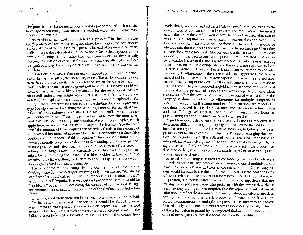
~he'@oiflt is $at chance guarantees a certain proportion of such associations; ajid when mahy associacioris are studied, many false positive asso- riaiioiis are po-ogible: The tl-adtianal statistical approach to this "problem" has been to make

.thz "sign-ific~ce',' test.more stringent, either by changing the criterion to a more stririgem'value, such ,&.l percent instead of 5 percent, or by actually infl~iiting the .calculated Pivalues by some factor that depends on the number of comparisons made: since epidemiologists, in their usually tliorough evaluation of expensively obtained data, typically make multiple Cdmpaiisons, they'have freq.uently been admonished to be wary of the problem. '.",

Ir is not clear, however, that the recommended solution is an improve- ment. In the fiist.place, the above argument, like all hypothesis testing, st&^^ from the premise that the kxpl~at ion for all the so-called "signifi- c-mt" results is chance, a sort of grarid null hypothesis. But why should we assuine that chance .is a likely explanation for the associations that are observed? ~iidged, one might argue that it seldom is (some would say never is) the'explq?t~on for findings. If chance is not the explanation for a "significantljr" posi'dve asso.ciationi then the finding does not represent a type' I or a l p h a - 2 r r o ~ . . ~ ~ making the screening criterion for statistical "significance" more stringent, a penalty is paid: Real non-null associations may go undetected (a type I1 error) because they fail to meet the more stringent rriteri.on. &I elementary consideration of screening principles, which apply here, mikes it c les that born a single criterion (the "significance" level) the num4er of false positives can be reduced only at the expense of an:increased frequency of false negatices. Is it worthwhile to reduce false pdisifives at the expimse of false. negatives? he question cannot be an- swei;ed, gelierdly; it requires a deepet understatlding of the consequences of false positive and false negative results in the context of the research setting. One thing, however, is exrremely clear Whatever the arguments migh~ be for reducing the chance of a false positive in favor of a false negative, they have nothing to do with multiple comparisons; they would apply equally well to a single comparison.

, The crux hffhe multiple comparison problem seems to be that in per- forn?iirrg m&iy &mptirisons m d reporting only those that are "statistically sign-ificarit," it is. d&cult to impute.the intended interpretation to the P- value; in the null hypothesis, a well-defined proportion of tests would be "significant;". but, if the denominator, the number of comparisons, is large arid ur&no%,.a reasonable interljretation of the P-values reported is hin- dered.

Lf many comparisons were made and each one were reported individually, let us say in a separate publication, it would be absurd to make adjhstments to the reported P-values in each report based on the total number of such reports. If such adjustments were indicated, it would also follow that an investigator should keep a cumulative total of comparisons

FUNDAMENTALS O F EPIDEMIOLOGIC DATA ANALYSIS 149

made during a career, and adjust all "significance" tests according to the current total of comparisons made to date. The more senior the investigator, the more the P-value would have to be inflated. For that matter, wouldn't such adjustments have to take into account the anticipated number of future comparisons as well as those already made? It should be obvious that these concerns are irrelevant to the research problem; they convert the P-value from a statistic conveying information about a specific association in the data to one that depends omthe unrelated experiences or psychologic state of the investigator. No one has yet suggested making adjustments for multiple comparisons if the results are reported individually in separate publications. But is it not inconsistent then to consider making such adjustments if the same results are aggregated into one or several publications? Would a review paper of individually reported associations have to adjust the P-values? If no adjustments should be made to P-values when they are reported individually in separate publications, it follows that the process of lumping the results together in one place should not affect the results themselves, regardless of when and how the lumping is done. Therefore, no adjustments for multiple comparisons should be made even if a large number of comparisons are reported at one time, provided that it is clear how many comparisons have been made and that all "negative" (that is, "nonsignificant") results have been reported along with the "positive" or "significant" results.

A problem does exist when the negative results are not reported; it is then more difficult to interpret properly the P-values for the positive findings that are reported. It is still a mistake, however, to believe that interpretation can be improved by adjusting the P-value or changing the criterion for "significance." The adjusted values are also impossible to interpret, since they divulge even less about the actual association; chang- Ing the criterion for "significance" does not actually solve the problem; as discussed earlier, it merely produces a smaller type I error at the expense of a greater type I1 error

As usual, some clarity is gained by considering the use of confidence intervals rather than "significance" tests. The equivalent of multiplying the P-value by some adjustment factor to compensate for multiple comparisons would be broadening the confidence interval. But the broader interval has no relation to the amount of information in the data about the effect in question; it depends instead on the number of comparisons that the investigator might have made. The problem with this approach is that it

j seems to defy the logical presumption that the reported results about an L effect should reflect the amount of information about the effect in the data, R nothing more and nothing less. If broader cofidence intervals were re- A o r t e d to compensate for multiple comparisons, a reader with an interest

focused solely on the one item would pay an unnecessary penalty in terms of the information imparted by the reported findings simply because the original investigator did not also focus solely on that problem.

since no problem calling for any Adjustments seems to exist unless the pasiiive results from, a large number.of comparisons are reported without

.in£orrnstion 'about the total number: df comparisons, and since even &eir,it appezrs that adjustments in the results dnly make them more dif-

. ficult t ~ ) inferpret, ,the best course forthe epidemiologist to take when ifl~aking multiple. ~omparisons. is. to ignore advice to make such adjust- menrs .in repor.tcd results. Each finding should be reported as if it alone were the soke hcus of a study. If a large number of comparisons makes it infeasible to report all findings, it is important to make it clear how many associations were: evaluated. If it cannot be determined how many comparisons were made, then associations not previously reported should be considered merely suggestive. It is worth emphasizing, however, that any new findings should always be considered only suggestive, even if only one. comparison is made. ~indirrgs. *at address a previously reported association or lack of Gsoc~ation should.not beco,me a weaker confirmation or refutation 'siniply because they are accompanied by many other unre- he: d cofiparisons, shce the previ~ously reported findingSon the question .mount to a prior hypothesis.

. . . REFERENCES

Brown, C. C. The .validity of approximate methods for interval estimation of the ' odds rati-o. ~ m . J! ~pideniol. 1981;113:47&480.

~dchrm, w. G. .The effectiveness of adjustment by subclassification in removing bias in oljskrvational studies. B i ~ m e ~ c s 1968;24:295-313.

Cornfield, J. A staristical problem arising from retrospective studies. In J. Neyman (ed.) Pro~eedings nird ~ e r k e l b Symposium, Vol. 4 . Berkeley: University of Cal- iforriia Press; 1956, pp. 135-148:

G&t, J. J. Statatistical 'analyses of the .reiative risk. Enuiron. Health Perspect. 1973;32:157-167.

Gart, J. J.., and Thomas, D. G. The performance of three approximate confidence limit methods for the odds ratio. Am. J. Epidemiol. 1982;115:45~70.

Greenlaid, S. A.counterexample to the test-based principle of setting confidence .limits. Am. J. Epideniiol. 1984;120:4-7:

Halperin, M. Re: 'rEstimability and estimation in case-control studies." Letter to the E#tor. Am. J. Epidmiol. 1977;105:49&498.

Lancasrer, H. 0.' The"combination of probabilities arising from data in discrete distributions. BiomeWika 1949;36:31&382.

Lancter, H. 0. Significance tests in discrete dishbutions. j. Am. Stat. ~ O C .

1961;46:223-234.. ~&laughlin, D. S. A data validatio;; .program nucleus. Comput. Prog. Biomed . .1~80;11:43-47.

Miettirien, 0.5. '~~dmability and estimation in ,case-referent studies. Am. J. Epide- miol. 1976a;103:226-235.

Mieninen, 0. S. Stratification by a nqltivariate confounder score. Am. J. Epidemiol. 1376b;104t609-620.


Miettinen, 0. S., and Nurminen, M. Comparative analysis of two rates. Statistics Med. 1985;4:213-226.

Rothrnan, K. J., and Keller, A. Z. The effect of joint exposure to alcohol and tobacco on risk of cancer of the mouth and pharynx. J. C ~ E . Dis. 1972;25:711-716.

Yates, F. Contigency cables involving small numbers and the chi-square test. J. R. Sfahkt SOC Suppl. 1934;1:217-235.

Documents

MODERN EPIDEMIOLOGY - McGill University · MODERN EPIDEMIOLOGY Professor, Department of Family and Community Medicine, University of Massachusetts Medical School, Worcester, Massachusetts