Modern Control Systems

(ECEG-4601)

Instructor: Andinet Negash

Chapter 1

Lecture 1: Mathematical

Model of Control Systems

Introduction

Definition:

The mathematical model of a dynamic system is a set of equations

that represents the dynamics of the system accurately or at least

fairly well

A one-component system

10/30/2013 2 Chapter 1: slide 1

Introduction

The equation:

Relates the physical quantities with the

component

Determining the system’s mathematical

model is essentially an approximation of the

behavior of a physical system with an ideal

mathematical expression.

Riv iv,

R

10/30/2013 3 Chapter 1: slide 1

Introduction

To have greater accuracy, one must take into account additional factors: for example, that the resistance R changes with temperature.

And, consequently, the relation should have the nonlinear form , where R(i) denotes that R is a nonlinear function of the current i.

However, it is well known that this more accurate model is still an approximation of the physical system.

In general, the mathematical model can only give an approximate description of a physical system.

Riv )(iRv

10/30/2013 4 Chapter 1: slide 1

Introduction

Simplicity Versus Accuracy.

Compromise between the simplicity of the model and the accuracy of the results of the analysis.

In deriving a reasonably simplified mathematical model, we frequently find it necessary to ignore certain inherent physical properties of the system.

If a linear lumped-parameter mathematical model (that is, one employing ordinary differential equations) is desired, it is always necessary to ignore certain nonlinearities and distributed parameters that may be present in the physical system.

If the effects that these ignored properties have on the response are small, good agreement will be obtained between the results of the analysis of a mathematical model and the physical system.

10/30/2013 5 Chapter 1: slide 1

Introduction

The problem of deriving the mathematical model of a system

usually appears as one of the following two cases.

1. Derivation of System’s Equations

2. System Identification

Derivation of System’s Equations

In this case, the system is considered known.

10/30/2013 6 Chapter 1: slide 1

Introduction

Here, we know the components R, L, C1, and C2 and their

interconnections.

To determine a mathematical model of the network, one may apply

Kirchhoff’s laws and write down that particular system of

equations which will constitute the mathematical model.

From network theory, it is well known that the systems of equations

sought are the linearly independent loop or node equations.

System Identification In this case the system is not known.

By ‘‘not known,’’ we mean that we do not know either the system’s

components or their interconnections.

The system is just a black box.

10/30/2013 7 Chapter 1: slide 1

Introduction

In certain cases, we may have available some apriori (in advance)

useful information about the system, e.g., that the system is time-

invariant or that it has lumped parameters, etc.

Based on this limited information about the system, we are asked to

determine a mathematical model which describes the given system

‘‘satisfactorily.’’

10/30/2013 8 Chapter 1: slide 1

Introduction

Here, both the physical system and the mathematical model are

excited by the same input u(t).

Subsequently, the difference e(t) of the respective responses y1and

y2 is measured.

If the error e(t) is within acceptable bounds, then the mathematical

model is a satisfactory description of the system.

The acceptable bounds depend on the desired degree of accuracy of

the model, and they are usually stated in terms of the minimum

value of the following cost function:

10/30/2013 9 Chapter 1: slide 1

1

0

)(2

t

t

dtteJ

Introduction

Types of Mathematical Models

Several types of mathematical models have been proposed for the description of systems.

1. The differential equations

2. The transfer function

3. The impulse response

4. The state equations.

There are other ways of describing a system, aiming to give a schematic overview of the system.

1. The block diagrams

2. The signal-flow graphs

10/30/2013 10 Chapter 1: slide 1

Introduction

Differential Equations

The mathematical model of differential equations (or, more

generally, of integro-differential equations) is the oldest method of

system description.

This description includes all the linearly independent equations of

the system, as well as the appropriate initial conditions.

Example 1:

10/30/2013 11 Chapter 1: slide 1

Introduction

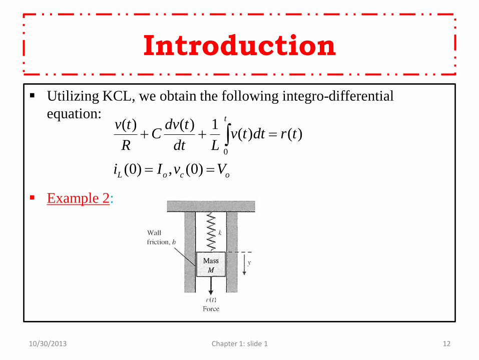
Utilizing KCL, we obtain the following integro-differential

equation:

Example 2:

10/30/2013 12 Chapter 1: slide 1

ocoL

t

VvIi

trdttvLdt

tdvC

R

tv

)0(,)0(

)()(1)()(

0

Introduction

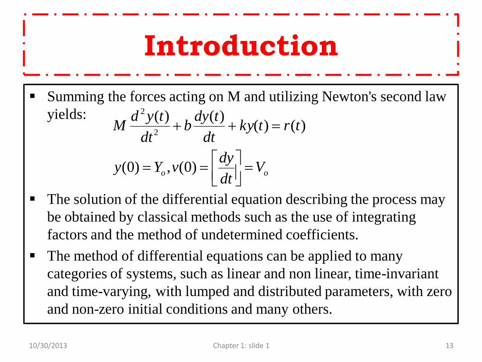
Summing the forces acting on M and utilizing Newton's second law

yields:

The solution of the differential equation describing the process may

be obtained by classical methods such as the use of integrating

factors and the method of undetermined coefficients.

The method of differential equations can be applied to many

categories of systems, such as linear and non linear, time-invariant

and time-varying, with lumped and distributed parameters, with zero

and non-zero initial conditions and many others.

10/30/2013 13 Chapter 1: slide 1

oo Vdt

dyvYy

trtkydt

tdyb

dt

tydM

)0(,)0(

)()()()(

2

2

Introduction

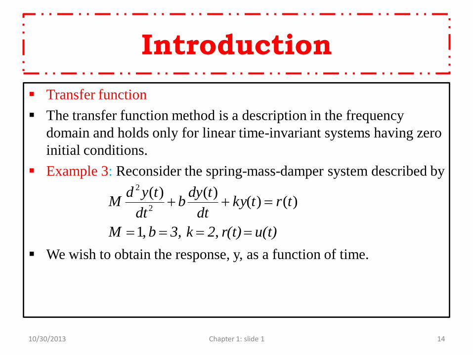
Transfer function

The transfer function method is a description in the frequency

domain and holds only for linear time-invariant systems having zero

initial conditions.

Example 3: Reconsider the spring-mass-damper system described by

We wish to obtain the response, y, as a function of time.

10/30/2013 14 Chapter 1: slide 1

u(t)r(t)23, kbM

trtkydt

tdyb

dt

tydM

, ,1

)()()()(

2

2

Introduction

The Laplace transform is:

Regrouping,

The response can be decomposed into two parts.

10/30/2013 15 Chapter 1: slide 1

)()(2)0()(3)0()0()(2 sUsYussYysysYs

response state-

2

responseinput -

2)(

23

1

23

)0()0()3()(

zerozero

sUssss

yyssY

Introduction

The first part is excited exclusively by the initial state and is called

zero-input response.

The second part is excited exclusively by the input and is called the

zero-state response.

Zero-input response – characteristic polynomial

If u(t)=0 for t0, then

This is called the homogeneous equation.

On application of Laplace transform, we obtain:

10/30/2013 16 Chapter 1: slide 1

0)(2)(

3)(

2

2

tydt

tdy

dt

tyd

Introduction

Whose solution is given as:

Where

is called the characteristic polynomial because it governs the free,

unforced or natural response of the system

10/30/2013 17 Chapter 1: slide 1

23

)0()0()3()(

2

ss

yyssY

)]0()0([

)0()0(2

)(

2

1

2

21

yyk

yykwhere

ekekty tt

232 ss

Introduction

Zero-state response: transfer function

Here, we have

Where the rational function:

is called the transfer function.

10/30/2013 18 Chapter 1: slide 1

)(23

1)(

2sU

sssY

23

1

)(

)()(

2

sssU

sYsG

00][

][

)(

)()(

ICIC

Input

Output

sU

sYsG

LL

Introduction

A transfer function may be defined only for a linear, stationary

(constant parameter) system.

A non stationary system, often called a time-varying system, has one

or more time-varying parameters, and the Laplace transformation

may not be utilized.

Furthermore, a transfer function is an input-output description of the

behavior of a system.

Thus, the transfer function description does not include any

information concerning the internal structure of the system and its

behavior.

10/30/2013 19 Chapter 1: slide 1

Introduction

Impulse-Response Function.

Consider the output (response) of a system to a unit-impulse input

when the initial conditions are zero.

Since the Laplace transform of the unit-impulse function is unity,

the Laplace transform of the output of the system is:

The inverse Laplace transform of G(s), or

is called the impulse-response function.

This function g(t) is also called the weighting function of the

system.

10/30/2013 20 Chapter 1: slide 1

)()( sGsY

)()(1 tgsG L

Introduction

The impulse-response function g(t) is thus the response of a linear

system to a unit- impulse input when the initial conditions are zero.

The Laplace transform of this function gives the transfer function.

Therefore, the transfer function and impulse-response function of a

linear, time-invariant system contain the same information about the

system dynamics.

It is hence possible to obtain complete information about the

dynamic characteristics of the system by exciting it with an impulse

input and measuring the response.

In practice, a pulse input with a very short duration compared with

the significant time constants of the system can be considered an

impulse

10/30/2013 21 Chapter 1: slide 1

Introduction

Linear Approximations of Physical Systems

A great majority of physical systems are linear within some range of

the variables.

In general, systems ultimately become nonlinear as the variables are

increased without limit.

For example, the spring-mass-damper system is linear and described

by the linear equation as long as the mass is subjected to small

deflections y(t).

However, if y(t) were continually increased, eventually the spring

would be over extended and break.

Therefore the question of linearity and the range of applicability

must be considered for each system.

10/30/2013 22 Chapter 1: slide 1

Introduction

The necessary condition for a linear system can be determined in

terms of an excitation x(t) and a response y(t).

1. Principle of Superposition:

2. Property of Homogeneity:

Example 4: Is the system represented by the following relation

linear? Which property is not satisfied?

10/30/2013 23 Chapter 1: slide 1

2121

22

11 then, yyxx

yx

yx

constant is );()( ),()( tytxthentytx

bmxy

Introduction

The above system may be considered linear about an operating point

x0,y0 for small changes Δx and Δy.

which satisfies the necessary conditions.

Consider the function

If the function is continuous over the range of interest with an

operating point x0 the Taylor series expansion about x0 will be:

10/30/2013 24 Chapter 1: slide 1

xmyor

bxmmxyybmxy

yyyxxx

,

or

and when,

00

00

)()( txgty

Introduction

If the dependent variable y depends upon several excitation

variables, then the functional relationship is written as:

The Taylor series expansion about the operating point x10 , x20 , x30 ,

… , x10 will be: [neglecting HOTs]

10/30/2013 25 Chapter 1: slide 1

!2

!1)()(

2

0

2

2

0

0

00

xx

dx

gdxx

dx

dgxgxgy

xxxx

n

xxxgy ,,,21

!1

!1

!1

),,( 0202

2

101

1

02010

000

nn

xxnxxxx

n

xx

dx

dgxx

dx

dgxx

dx

dgxxxgy

Introduction

Example 5: Consider the pendulum oscillator shown below. The

torque on the mass is T=MgLsinθ where g is the gravity constant.

The equilibrium condition for the mass is θ0=0°. The nonlinear

relation between T and θ is shown graphically.

10/30/2013 26 Chapter 1: slide 1

Introduction

The first derivative evaluated at equilibrium provides the linear

approximation, which is:

This approximation is reasonably accurate for π/4<0<π/4.

For example, the response of the linear model for the swing through

±30° is within 5 % of the actual nonlinear pendulum response.

10/30/2013 27 Chapter 1: slide 1

MgLMgLT

TMgLTT

00cos

0 where;sin

000

0

Introduction

Further Reading:

Identify proper/improper/biproper rational functions.

Revise on the following topics:

The Laplace transform

Solutions of first and second order ODE

For the next lecture revise the following topics:

Matrices

10/30/2013 28 Chapter 1: slide 1