Embed Size (px)
Citation preview

Models with Nominal Rigidities
Karel Mertens, Cornell University
Contents
1 Monopolistic Competition 3
2 One-Period Sticky Prices 9
3 Staggered Price Setting: The Calvo Model 14
4 A Basic Model of the Effects of Monetary Policy 21
References
Bullard, J. and Mitra, K. (2002), ‘Learning about monetary policy rules’, Journal of Mon-
etary Economics (6), 1105–1129.
Calvo, G. A. (1983), ‘Staggered prices in a utility maximizing framework’, Journal of Mon-
etary Economics (3), 383–398.
Gali, J., Gertler, M. and Lopez-Salido, J. D. (2001), ‘European inflation dynamics’, Euro-
pean Economic Review (7), 1237–1270.
Taylor, J. B. (1993), ‘Discretion versus policy rules in practice’, Carnegie-Rochester Con-
ference Series on Public Policy (1), 195–214.
Walsh, C. E. (2003), Monetary Theory and Policy, 2nd Ed., MIT Press. Ch 5.4.
Woodford, M. (2003), Interest and Prices: Foundations of a Theory of Monetary Policy,
Princeton Press. Ch 3, 4.
1

Introduction
In the chapter on flexible price monetary models, we saw that the MIU, CIA and ST
models can generate real effects to monetary disturbances. However, these effects were
qualitatively inconsistent with the empirical evidence produced for instance by monetary
structural VARs. In most cases, the responses of the real variables in realistic simulations
were also quantitatively so insignificant that money basically did not matter in practice.
This chapter presents some alternative models in which there are significant and empirically
plausible short-run effects of monetary disturbances. These models are important tools for
understanding how monetary policy and other aggregate demand shocks affect economic
behavior and the business cycle.
There are generally three classes of models that are relatively successful in reconciling the
long-run neutrality of money with the apparent short-run nonneutrality: the first two are
models of imperfect information and models of limited participation, both of which maintain
the assumption of flexible prices. The third, and arguably most popular, class of models
incorporate nominal rigidities, either in the form of sticky goods prices or sticky nominal
wages. This chapter will focus exclusively on sticky price models.
In the next section we will take a very simple dynamic general equilibrium model and
introduce monopolistic composition, an essential ingredient for most sticky price model. The
second section introduces the simplest form of price stickiness: one period preset prices. The
third section introduces a more realistic model of staggered price setting. The fourth section
discusses a benchmark model that can be used for the analysis of monetary policy. The
final section discusses the microeconomic evidence for nominal price rigidities.
2

1 Monopolistic Competition
This section extends a basic MIU model by allowing for monopolistic competition in the
goods market. Introducing some degree of monopoly power is essential to allow firms to
set their own prices. For simplicity, the model abstracts from capital accumulation. You
can think of capital being used in production, but capital goods are in fixed supply, do not
depreciate and their allocation across households (or firms) cannot be changed.
Households The economy is populated by a representative household with preferences
represented by
U = E0
∞∑t=0
βtu(Ct, 1−Nt,mt) , 0 < β < 1 (1)
where Nt is labor and mt =MtPt
is the real value of money holdings, Mt > 0 denotes nominal
money balances. There is a continuum of consumption goods distributed uniformly over the
unit interval. Ct is a composite consumption index given by the Dixit-Stiglitz aggregator
Ct =
[∫ 1
0Ct(i)
θ−1θ di
] θθ−1
, θ > 1
where Ct(i) is the quantity of good i ∈ [0, 1] consumed in period t and θ is the elasticity of
substitution among consumption goods. Pt is the corresponding utility-based price index of
the prices of all goods. It is defined as the minimum amount of nominal spending required
to obtain (at least) one unit of Ct. In the expenditure minimization problem:
minct(i)
∫ 1
0Pt(i)Ct(i)di s.t. Ct ≥ 1
Pt is the Lagrange multiplier on the constraint. The first order condition to this problem
is
Pt(i) = Pt
(Ct(i)
Ct
)− 1θ
(2a)
⇔ Ct(i) =
(Pt(i)
Pt
)−θ
Ct (2b)
3

together with Ct = 1. Substituting (2a) into the objective function, we have∫ 1
0Pt(i)Ct(i)di = Pt
(∫ 1
0Ct(i)
θ−1θ di
)C
1θt
= PtCθ−1θ
t C1θt
= PtCt
= Pt
Substituting (2b) into the objective function, we have that
Pt =
(∫ 1
0Pt(i)
1−θdi
) 11−θ
which is called the Dixit-Stiglitz price index. It implies that total nominal consumption
expenditure equals PtCt. The household’s period budget constraint is:∫ 1
0Pt(i)Ct(i)di+Bt +Mt ≤ WtNt +Mt−1 + (1 +Rt−1)Bt−1 + Tt +Qt
where Pt(i) is the nominal price of good i, Wt is the nominal wage, Tt are lump-sum
monetary transfers by the government, Bt are government issued bonds and Qt are nominal
profits from firm ownership. Utility maximization implies that the households will solve the
expenditure minimization problem above to decide on the optimal intratemporal allocation
of the different consumption goods. The budget constraint relevant for the intertemporal
problem can be reduced to
PtCt +Bt +Mt ≤ WtNt +Mt−1 + (1 +Rt−1)Bt−1 + Tt +Qt
The household’s intertemporal problem is to choose the real quantities {Ct,mt, Nt}∞t=0 to
maximize (1) subject to the budget constraints for a given level of initial money holdings
and taking as given prices, monetary transfers and firm profits.
As seen previously, the household’s first order conditions lead to
uc(Ct,mt, 1−Nt) = βEt
[uc(Ct+1,mt+1, 1−Nt+1)
1 +Rt
1 + πt+1
]um(Ct,mt, 1−Nt)
uc(Ct,mt, 1−Nt)=
Rt
1 +Rt
uc(Ct,mt, 1−Nt)wt = ul(Ct,mt, 1−Nt)
4

where wt =WtPt
is the real wage.
Firms There is a continuum of firms in the economy that are uniformly distributed over
the unit interval. Each firm is indexed by i ∈ [0, 1] and produces a differentiated good using
the technology
Yt(i) = AtNαt (i) , 0 < α < 1, A > 0 (3)
Yt(i) is output of firm i and Nt(i) is the quantity of labor used by firm i. At is a random
stationary productivity process common to all firms. Labor input is rented in a competitive
market at a real wage wt. Each firm acknowledges how the demand for its differentiated
good i depends on its own price level Pt(i)
Yt(i) = Ct(i) =
(Pt(i)
Pt
)−θ
Ct (4)
At the same time, the individual firm regards itself as unable to affect the evolution of the
variables Ct and Pt and takes these as given.
As there is no intertemporal dimension to the firm’s problem, the optimal Pt(i) will
maximize period t profits
Qt(i)
Pt=
Pt(i)
PtYt(i)− wtNt(i)
=
(Pt(i)
Pt
)1−θ
Ct −wt
A1αt
(Pt(i)
Pt
)−θα
C1αt
Optimal price setting requires
(1− θ)
(Pt(i)
Pt
)−θ Ct
Pt+
wt
A1αt
θ
α
(Pt(i)
Pt
)− θα−1 C
1αt
Pt= 0
⇔ (1− θ)Yt(i) +θ
αwtNt(i)
Pt
Pt(i)= 0
⇔ (1− θ)Pt(i)Yt(i) +θ
αWtNt(i) = 0
⇔ Pt(i) =θ
θ − 1
WtNt(i)
αYt(i)
The optimal price setting condition implies a fixed markup over the marginal cost of pro-
5

duction, i.e.
Pt(i) = ωMCt(i)
where ω = θθ−1 > 1 is the constant markup and MCt(i) =
WtNt(i)αYt(i)
is the marginal cost of
production. Note that as θ → ∞, the goods become perfect substitutes and the markup
goes to one. MCt(i) is defined as the Lagrange multiplier in the cost minimization problem
minNt(i)
WtNt(i) s.t. Yt(i) ≥ Y
The first order condition is
Wt = MCt(i)αAt(Nt(i))α−1
⇔ MCt(i) =WtNt(i)
αYt(i)
Government The government is the monopoly supplier of money, which it uses to finance
the lump-sum transfers and supplies a fixed amount of nominal bonds. Assume that the
growth rate of the money supply in deviation of the steady state growth rate, denoted by
θt =Mt
Mt−1−µ−1 is an stationary mean zero exogenous random variable and µ is the average
money growth rate.
Equilibrium In a symmetric equilibrium, all firms maximize profits and choose identical
prices (Pt(i) = Pt , ∀i) and labor input levels (Nt(i) = Nt , ∀i), households solve their
utility maximization problem and all markets (for goods, assets and labor) clear.
Model Dynamics We will assume the following simple functional form for the instanta-
neous utility function:
u(Ct, 1−Nt,mt) = u(Ct, Nt,mt) =C1−σt
1− σ+ ϕm
m1−χt
1− χ− ϕn
N1+ξt
1 + ξ, σ, χ, ξ, ϕm, ϕn > 0
6

The dynamics of aggregate consumption Ct, hours Nt, output Yt and real money balances
mt can be summarized by the following conditions:
1 = βEt
[(Ct+1
Ct
)−σ 1 +Rt
1 + πt+1
](5a)
Yt = Ct (5b)
ϕmmt−χ =
Rt
1 +RtC−σt (5c)
mt
mt−1(1 + πt) = 1 + µ+ θt (5d)
ϕnNξt =
α
ω
YtNt
C−σt (5e)
Yt = AtNαt (5f)
Equation (5a) and (5b) can be combined to derive an IS-relationship between output and
the interest rate that represents goods market clearing:
Y −σt =βEt
[Y −σt+1
1 +Rt
1 + πt+1
](6a)
Equation (5b), (5c) and (5d) can be combined to derive an LM-relationship between output
and the interest rate that represents asset market clearing:
Rt
1 +Rt=ϕm
(1 + µ+ θt1 + πt
mt−1
)−χ
Y σt (6b)
Finally, combine (5e) and (5f) to get aggregate supply AS:
Yt = A1+ξ
1+ξ+α(σ−1)
t
(α
ϕnω
) α1+ξ+α(σ−1)
(6c)
Equation (6a) to (6c) constitute a very tractable flexible price macroeconomic model with
one aggregate supply shock At and one aggregate demand shock θt.
Consider the following loglinear approximations:
yt =Etyt+1 −1
σ
(Rt − Etπt+1
)(IS)
σyt =χ(θt + mt−1 − πt) +β
1 + µ− βRt (LM)
yt =1 + ξ
1 + ξ + α(σ − 1)at (AS)
7

Figure 1: Flexible Price Model: i.i.d. shocks
1 2 3 4 5 6−0.2
0
0.2
0.4
0.6
0.8
1
1.2
Per
cent
Dev
iatio
ns
Quarters
Money Growth Shock
ymRπaθ
1 2 3 4 5 6−1
−0.5
0
0.5
1
Per
cent
Dev
iatio
ns
Quarters
Technology Shock
ymRπaθ
Figure 2: Flexible Price Model: persistentshocks
1 2 3 4 5 6−1
−0.5
0
0.5
1
1.5
2
Per
cent
Dev
iatio
ns
Quarters
Money Growth Shock
ymRπaθ
1 2 3 4 5 6−1
−0.5
0
0.5
1
Per
cent
Dev
iatio
ns
Quarters
Technology Shock
ymRπaθ
Consider the following simple parametrization of the model: α = 0.58, β = 0.988, σ = 1,
ξ = 1, χ = 10, µ = 0. At this point, it is not necessary to specify values for the other
parameters as they do not influence the model dynamics. Note for instance that the value
of θ, the elasticity of substitution among goods, only affects the long run level of output
but not the short-run dynamics. To improve our understanding of the model, Figure 1
plots the impulse responses to a money growth and technology shock under the assumption
that both are i.i.d. random variables. First consider the money growth shock: the model
displays monetary neutrality and superneutrality in both the short and long run and the
AS curve is perfectly vertical, i.e. we obtain the classical dichotomy. This implies that
AD-shocks such as an increase in the money growth rate cannot change output which is
8

always at its long run natural level given by equation (6c). Because the money shock is
i.i.d., there is no change in expected inflation or the nominal interest rate and prices move
one for one with the expanded money supply.
In response to a positive innovation in productivity, the natural output level increases, the
AS curve shifts out and the price level drops. In the period after the shock the AS curve
returns to its initial position and so does the price level. As a result of the decline in the
price level in the period of the shock the LM curve shifts out, real money balances increase
and the nominal interest rate declines. After the shock, the price level goes back up and
the LM curve returns to its initial position.
Figure 2 plots the impulse responses to a money growth and technology shock under the
assumption that both shocks are persistent. As in the previous chapters, both follow AR(1)
processes with the persistence of θ equal to ρθ = 0.48 and the persistence of the technology
shock equal to ρa = 0.9. After a money growth shock, the additional effects that come into
play are because of a change in expected inflation. The drop in real money demand implies
that the price level must increase more than proportional to the money supply, such that
real money balances drop. The nominal interest rate increases: there is no (dominating)
liquidity effect.
After a persistent increase in productivity, the price level is slow to return to its initial
level as the natural level output is now persistently higher. The effects of higher expected
inflation that reduce demand for real money balances (LM curve shifts to the right) together
with the effect of future higher expected output on consumption (IS curve shifts to the right)
make the initial drop in the price level smaller than in the i.i.d case.
The Matlab-program used to compute these impulse responses is stickyprice1.m.
2 One-Period Sticky Prices
Now suppose the firms must set their prices one period in advance, such that period t
prices do not react to the realizations of the period t demand and supply shocks. Assume
that firms are committed to supply whatever quantity buyers may wish to purchase at the
predetermined price, and hence firms obtain whatever labor input is necessary to fill orders.
The optimal Pt(i) which is set in period t− 1 maximizes the discounted value of expected
9

profits
Et−1
[β
λt
λt−1
Qt
Pt
]= Et−1
[β
λt
λt−1
(Pt(i)
PtYt(i)− wtNt(i)
)]
= Et−1
β λt
λt−1
(Pt(i)
Pt
)1−θ
Ct −wt
A1αt
(Pt(i)
Pt
)−θα
C1αt
Optimal price setting requires
Et−1
λt
(1− θ)
(Pt(i)
Pt
)−θ Ct
Pt+
wt
A1αt
θ
α
(Pt(i)
Pt
)− θα−1 C
1αt
Pt
= 0
⇔ Et−1
[λt
((1− θ)
Pt(i)
PtYt(i) +
θ
αwtNt(i)
)]= 0
⇔ Et−1
[λt
(Pt(i)
PtYt(i)−
ω
αwtNt(i)
)]= 0
⇔ Et−1
[λtYt(i)
(Pt(i)
Pt− ω
MCt(i)
Pt
)]= 0
In a symmetric equilibrium in which all firms set identical prices and chose the same number
of hours, the optimal price setting condition reduces to
⇔ Et−1
[Y 1−σt
(1− ω
MCt
Pt
)]= 0
⇔ Et−1
[(Y 1−σt − ωϕn
αN1+ξ
t
)]= 0
⇔ Et−1
[(Y 1−σt − ωϕn
αA
− 1+ξα
t Y1+ξα
t
)]= 0
⇔ Et−1
[Y 1−σt
(1− ωϕn
αA
− 1+ξα
t Y1+ξ+α(σ−1)
αt
)]= 0
⇔ Et−1
Y 1−σt
1−(
YtY nt
) 1+ξ+α(σ−1)α
= 0 (7)
where Y nt is defined as the natural level of output which equals the level of output that
would prevail in the flexible price economy, i.e.
Y nt = A
1+ξ1+ξ+α(σ−1)
t
(α
ϕnω
) α1+ξ+α(σ−1)
(8)
10

It is appropriate to think of (7) as the short-run aggregate supply curve and (8) as the long
run aggregate supply curve. Loglinearizing yields the following aggregate supply relation-
ships:
Et−1 [yt − ynt ] = 0 (SRAS)
ynt =1 + ξ
1 + ξ + α(σ − 1)at (LRAS)
where yt − ynt is called the output gap. The SRAS and LRAS, together with the IS-LM
equations of the previous section determine the dynamics of the endogenous variables.
Note that the labor supply equation (and the value of the wage elasticity!) is irrelevant
in determining the short-run equilibrium level of output. Any unanticipated movements in
aggregate demand are met by varying the nominal wage such as to supply the required level
of goods: the SRAS aggregate supply curve is horizontal at the preset price level and output
may deviate from the natural level. In the short run, the level of output is determined by
aggregate demand only. As a result, in the sticky price model, money will neither be neutral
nor superneutral in the short run.
Consider the same parametrization of the model as before: α = 0.58, β = 0.988, σ = 1,
ξ = 1, χ = 10 and µ = 0. Again, it is not necessary to specify values for any other
parameters since they do not influence the model dynamics. Note that the steady state and
the natural level of output are identical to the flexible price economy from the last section.
Figure 3 plots the impulse responses to a money growth and technology shock in the sticky
price model for the case where the shocks are i.i.d. Contrary to the flexible price model,
money is no longer neutral: output expands after a positive money growth shock. At fixed
prices, equilibrium in the market for money now requires a lower nominal interest rate to
equate money supply to money demand: the LM curve shifts to the right and so does the
AD curve. Note that the sticky price model delivers a liquidity effect. Firms cannot change
prices and meet the increased demand by increasing the nominal wage, labor input and
production. The implied drop in profits constitutes another reason why it was necessary to
introduce monopolistic competition and excess profits. In the period after the shock, prices
readjust, the LM curve and AD curves shift back to their original positions and output is
back at its natural level.
In response to a technology shock, there is no change in output, nor in either of the other
variables plotted. Since there is no change in aggregate demand, firms supply the quantity
demanded at current prices. As a result of the productivity improvement, they will be able
11
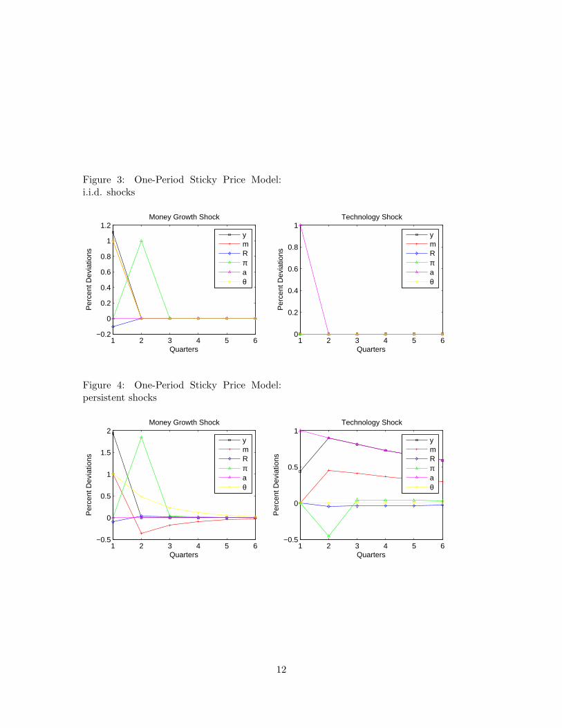
Figure 3: One-Period Sticky Price Model:i.i.d. shocks
1 2 3 4 5 6−0.2
0
0.2
0.4
0.6
0.8
1
1.2
Per
cent
Dev
iatio
ns
Quarters
Money Growth Shock
ymRπaθ
1 2 3 4 5 60
0.2
0.4
0.6
0.8
1
Per
cent
Dev
iatio
ns
Quarters
Technology Shock
ymRπaθ
Figure 4: One-Period Sticky Price Model:persistent shocks
1 2 3 4 5 6−0.5
0
0.5
1
1.5
2
Per
cent
Dev
iatio
ns
Quarters
Money Growth Shock
ymRπaθ
1 2 3 4 5 6−0.5
0
0.5
1
Per
cent
Dev
iatio
ns
Quarters
Technology Shock
ymRπaθ
12

to produce the same quantity with less labor input, so the nominal wage drops and hours
worked decrease.
Figure 3 plots the impulse responses to a money growth and technology shock in the sticky
price model for the case where the shocks are persistent: as before, ρθ = 0.48 and ρa = 0.9.
In response to the money growth shock, there is a drop in demand for real money balances
due to higher expected inflation. This additional effect further shifts out the LM curve and
the liquidity effect is larger. As a results, the increase in aggregate demand is larger if the
shock is persistent, and output expands more. The real effects are very transitory however:
the period after the shock the price adjust and output returns to its natural level. From
the second period onwards, the dynamics are identical to the case of flexible prices.
In response to a persistent productivity improvement, lower expected inflation shifts the LM
curve to the left and reduces aggregate demand, but higher future income shifts the is curve
to the right and increases aggregate demand. The real interest rate must unambiguously
increase, but there are offsetting effects on aggregate demand. It turns out that the future
income effect dominates such that the AD curve shifts the right in the period of the shock.
After one period prices adjust and the dynamics are the same as in the flexible price case.
The Matlab-program used to compute these impulse responses is stickyprice2.m.
13

3 Staggered Price Setting: The Calvo Model
This section presents a version of a model with staggered price setting introduced by Calvo
(1983). The section is based on Chapter 3 of Woodford (2003) and Chapter 5.4 of Walsh
(2003).
Staggered pricesetting In the Calvo model, a fraction γ of goods prices remain un-
changed each period, whereas a fraction 1−γ of firms chose new prices for their goods. For
simplicity, the probability that any given price can adjust is 1 − γ and is independent of
the length of time since the price was last adjusted. Each supplier that chooses a new price
for its good in period t faces exactly the same decision problem and the optimal price P ∗t
chosen is the same for all of them in equilibrium. The remaining fraction γ of prices are a
subset of the prices charged in t − 1. Given the assumption that every price has the same
probability of being changed, each price appears in the period t distribution of unchanged
prices with the same relative frequency as in the period t − 1 distribution of prices. This
allows us to write the Dixit Stiglitz price index as
Pt =
((1− γ)(P ∗
t )1−θ + γ
∫ 1
0Pt−1(i)
1−θdi
) 11−θ
=((1− γ)(P ∗
t )1−θ + γP 1−θ
t−1
) 11−θ
(9)
So in order to find Pt it suffices to know the new optimal price P ∗t and the price level in
period t− 1, Pt−1.
A firm that changes its price in period t maximizes expected discounted profits
Et
[ ∞∑s=t
(βγ)s−tλs
λt
(Pt(i)
PsYs(i)− wsNs(i)
)]
= Et
[ ∞∑s=t
(βγ)s−tλs
λt
((Pt(i)
Ps
)1−θ
Cs −ws
A1αs
(Pt(i)
Ps
)−θα
C1αs
)]
Optimal price-setting requires
Et
[ ∞∑s=t
(βγ)s−tλs
λt
((1− θ)
Pt(i)
PsYs(i) +
θ
αwsNs(i)
)]= 0
⇔ Et
[ ∞∑s=t
(βγ)s−tλs
λtYs(i)
(Pt(i)
Ps− ω
MCs(i)
Ps
)]= 0
14

In equilibrium Pt(i) = P ∗t such that
Et
[ ∞∑s=t
(βγ)s−tλsYts
(P ∗t
Ps− ω
MCts
Ps
)]= 0
where Y ts =
(P ∗t
Ps
)−θYs is period s output of a firm that last set its price in period t,
Ys =(∫ 1
0 Ys(i)θ−1θ di
) θθ−1
and MCts =
Wsα A
− 1α
s Y ts
1−αα is the period s marginal cost of a firm
that last set its price in period t. Furthermore,
Et
[ ∞∑s=t
(βγ)s−t
(P ∗t
Ps
)−θ
Y 1−σs
(P ∗t
Ps− ω
MCts
Ps
)]= 0
⇔ Et
[ ∞∑s=t
(βγ)s−t
(P ∗t
Ps
)1−θ
Y 1−σs
]= Et
[ ∞∑s=t
(βγ)s−t
(P ∗t
Ps
)−θ
Y 1−σs ω
MCts
Ps
]
⇔ Et
[ ∞∑s=t
(βγ)s−t
(Pt
Ps
)1−θ
Y 1−σs
]=
Pt
P ∗t
ωEt
[ ∞∑s=t
(βγ)s−t
(Pt
Ps
)−θ
Y 1−σs
MCts
Ps
]
such that the price of re-optimizing firms is given by
P ∗t
Pt= ω
Et
[∑∞s=t (βγ)
s−t(PsPt
)θY 1−σs
MCts
Ps
]Et
[∑∞s=t (βγ)
s−t(PsPt
)θ−1Y 1−σs
] (10)
The New Keynesian Phillips curve Defining p∗t =P ∗t
Ptand mcts =
MCts
Ps, we can rewrite
(10) as
p∗t =ω
1 + πt
Et
[∑∞s=t (βγ)
s−t(Πs−t
j=0(1 + πt+j))θ
Y 1−σs mcts
]Et
[∑∞s=t (βγ)
s−t(Πs−t
j=0(1 + πt+j))θ−1
Y 1−σs
]We will loglinearize this expression around a steady with has zero inflation (with µ = 0),
such that p∗ = 1 (see Woodford (2003) for a discussion, footnote 32 on p.179). Log-
linearizing the numerator on the right hand side yields
(1− βγ)Et
∞∑s=t
(βγ)s−t
(1− σ)ys + mcts +s−t∑j=0
θπt+j
15

Log-linearizing the denominator on the right hand side yields
(1− βγ)Et
∞∑s=t
(βγ)s−t
(1− σ)ys +
s−t∑j=0
(θ − 1)πt+j
Therefore, the loglinear version of (10) is
p∗t + πt = (1− βγ)Et
∞∑s=t
(βγ)s−t
mcts +s−t∑j=0
πt+j
= (1− βγ)
(mctt + πt
)+ βγ
πt + (1− βγ)Et
∞∑s=t+1
(βγ)s−t−1
mcts +s−t−1∑j=0
πt+1+j
(11)
Recall that mcts is the period s real marginal cost of a firm that re-optimizes in period t:
mcts =ws
αA
− 1α
s Y ts
1−αα
=ws
αA
− 1α
s
(P ∗t
Ps
)−θ 1−αα
Y1−αα
s
= mcs(p∗t )
−θ 1−αα
(Πs−t
j=0(1 + πt+j)
1 + πt
)θ 1−αα
where mcs = wsα A
− 1α
s Y1−αα
s is the “average” real marginal cost in period s. Loglinearizing
this expression yields
mcts = mcs − θ1− α
αp∗t + θ
1− α
α
s−t∑j=0
πt+j
− θ1− α
απt (12)
Substituting (12) in (11) yields
p∗t + πt = (1− βγ)
(mct − θ
1− α
αp∗t + πt
)+ βγπt
+βγ(1− βγ)Et
[∞∑
s=t+1
(βγ)s−t−1
(mcs − θ
1− α
αp∗t +
(1 + θ
1− α
α
) s−t−1∑j=0
πt+1+j
)](1 + θ
1− α
α
)p∗t = (1− βγ)mct + βγ(1− βγ)Et
[∞∑
s=t+1
(βγ)s−t−1
(mcs +
(1 + θ
1− α
α
) s−t−1∑j=0
πt+1+j
)](1 + θ
1− α
α
)p∗t = (1− βγ)mct + βγ
(1 + θ
1− α
α
)Et [p
∗t+1 + πt+1] (13)
16

To understand the last step, verify that
mct+1s = mcs − θ
1− α
αp∗t+1 + θ
1− α
α
(s−t−1∑j=0
πt+1+j
)− θ
1− α
απt+1
⇔ mct+1s +
s−t−1∑j=0
πt+1+j = mcs − θ1− α
αp∗t+1 +
(1 + θ
1− α
α
)(s−t−1∑j=0
πt+1+j
)− θ
1− α
απt+1
⇔ mcs +
(1 + θ
1− α
α
)(s−t−1∑j=0
πt+1+j
)= mct+1
s +
s−t−1∑j=0
πt+1+j + θ1− α
α(p∗t+1 + πt+1)
and that
βγ(1− βγ)Et
[∞∑
s=t+1
(βγ)s−t−1
(mcs +
(1 + θ
1− α
α
) s−t−1∑j=0
πt+1+j
)]
= βγ(1− βγ)Et
[∞∑
s=t+1
(βγ)s−t−1
(mct+1
s +
s−t−1∑j=0
πt+1+j + θ1− α
α(p∗t+1 + πt+1)
)]
= βγ
(1 + θ
1− α
α
)Et [p
∗t+1 + πt+1]
Next reconsider equation (9):
Pt =((1− γ)(P ∗
t )1−θ + γP 1−θ
t−1
) 11−θ
⇔ 1 = (1− γ)(p∗t )1−θ + γ(1 + πt)
θ−1
Loglinearizing this last expression yields
p∗t =γ
1− γπt (14)
Substituting (14) into (13) yields an expression for the evolution of aggregate inflation
known as the New Keynesian Phillips curve:
πt = κmct + βEt [πt+1] (15)
where κ = (1−βγ)(1−γ)
γ(1+θ 1−αα )
> 0, 0 < β < 1. In contrast to more traditional Phillips curves, the
New Keynesian Phillips curve implies that the (average) real marginal cost is the correct
driving variable for the inflation process and that inflation is forward looking, with current
inflation a function of expected future inflation. When a firm sets a price in the Calvo
framework, it is concerned about the future evolution of prices as it is unable to alter its
own price for a number of periods. Solving (15) forward, it is clear that inflation equals the
17

present discounted value of current and future real marginal costs:
πt = κEt
∞∑s=t
βs−tmcs
The parameter κ measures the impact of period t real marginal cost on period t inflation
and is a function of the structural parameters β, the discount factor, γ, the fraction of firms
that cannot change their prices, θ, the elasticity of substitution among consumption goods
and α, the curvature of the production function. Higher β lowers κ and means that the
firm gives more weight to future expected profits. More nominal price rigidity (higher γ)
reduces the sensitivity of current inflation to current marginal cost. The parameter κ is
also decreasing in the curvature of the production function as measured by α and in the
elasticity of demand θ. The larger α and θ, the more sensitive is the marginal cost of an
individual firm to deviations of its price from the average price level: everything else equal,
a smaller adjustment in price is desireable in order to offset expected movements in average
marginal costs.
Aggregate Supply From the definition of average real marginal cost and the household’s
labor supply condition, we have
mct =ϕnN
ξt
Y −σt
Nt
αYt
Recall that Yt was defined as
Yt =
(∫ 1
0Yt(i)
θ−1θ di
) θθ−1
= At
(∫ 1
0Nt(i)
α θ−1θ di
) θθ−1
As a first order approximation, we have
yt = at + αnt
18

Using this insight we can write
mct = (1 + ξ)nt + (σ − 1)yt
= −1 + ξ
αat +
(1 + ξ
α+ σ − 1
)yt
=1 + ξ + α(σ − 1)
α(yt − ynt )
such that the aggregate supply equation in the Calvo model becomes
πt = κ1 + ξ + α(σ − 1)
α(yt − ynt ) + βEt [πt+1] (16)
Model Analysis Consider the same parametrization of the model as before: α = 0.58,
β = 0.988, σ = 1, ξ = 1, χ = 10 and µ = 0. Now we have also have to choose a value
for θ since it will affect the slope of the aggregate supply curve. In addition, there is the
parameter γ measuring the degree if price rigidity. Gali, Gertler and Lopez-Salido (2001),
set ω = 1.10 (or θ = 11) and estimate a Phillips curve as in (15) using quarterly US data
to obtain a value of γ = 0.475. This estimate implies that the average duration of price
rigidity 11−γ is approximately two quarters.
Figure 5 illustrates the impact of a money growth and technology shock for the case where
both the shocks are i.i.d. It is evident that with staggered price setting inflation responds
sluggishly to economic shocks. In the case of a money growth shock, the initial impact on
prices is less proportional to the increase in the money supply, since only a fraction of goods
prices are adjusted. In subsequent periods, as more and more firms reset prices, the LM-
curve and AD curve return to their initial positions, but only gradually so. The persistent
output increase and slow response of inflation, together with the decrease in the nominal
interest rate after a monetary expansion are now more consistent with the evidence from
the structural VAR literature.
In contrast to the model with one period pre-set prices, output now increases after a positive
technology shock, albeit much less so then in the flexible price model. This is because now a
fraction of the firms can change prices in order to benefit from the technology improvement.
Figure 6 displays the responses to persistent money growth and technology shocks: as
before, ρθ = 0.48 and ρa = 0.9. After a persistent money growth shock, the effect of higher
anticipated future inflation further stimulates aggregate demand and the output increase
is now larger. In response to a persistent technology shock, the combination of aggregate
supply effects and aggregate demand effects (through inflation, expected future inflation
19

Figure 5: Calvo Sticky Price Model: i.i.d.shocks
1 2 3 4 5 6−0.2
0
0.2
0.4
0.6
0.8
1
1.2
Per
cent
Dev
iatio
ns
Quarters
Money Growth Shock
ymRπaθ
1 2 3 4 5 6−0.2
0
0.2
0.4
0.6
0.8
1
1.2
Per
cent
Dev
iatio
ns
Quarters
Technology Shock
ymRπaθ
Figure 6: Calvo Sticky Price Model: persis-tent shocks
1 2 3 4 5 6−0.5
0
0.5
1
1.5
Per
cent
Dev
iatio
ns
Quarters
Money Growth Shock
ymRπaθ
1 2 3 4 5 6−0.2
0
0.2
0.4
0.6
0.8
1
1.2
Per
cent
Dev
iatio
ns
Quarters
Technology Shock
ymRπaθ
20

and expected future output) generates a hump-shaped response of output.
The Matlab-program used to compute these impulse responses is stickyprice3.m.
4 A Basic Model of the Effects of Monetary Policy
This section introduces a more realistic formulation of monetary policy into the Calvo
staggered pricing model of the previous section. Recall that up until now, we have modeled
monetary policy in a very simplified manner by positing a random stochastic process for
the growth rate of the money supply. In this section, we will think of the government, or
central bank, as implementing monetary policy through control of the nominal interest rate.
Taylor Rule Monetary policy might be specified by a Taylor rule of the form
1 +Rt
1 + R= Ψ
(1 +Rt−1
1 + R,1 + πt1 + π∗ ,
YtY nt
, eϵi
t
)where Ψ(1, 1, 1, 1) = 1, π∗ is a target inflation rate and ϵRt is an exogenous mean zero
disturbance to the monetary rule. A rule of this form was first introduced by Taylor (1993)
and has proven to be a reasonable empirical description of the behavior of many central
banks. In loglinear form we may write the Taylor rule as
Rt = ρRRt−1 + (1− ρR) (ρππt + ρyxt) + ϵRt (17a)
where 0 ≤ ρR < 1, ρπ, ρy ≥ 0. The parameter ρR captures policy inertia that may be due
to the policy makers’ preference for interest rate smoothing. The coefficients ρπ, resp. ρy
measure the policymakers’ response to deviations of inflation from the target (steady state)
level, resp. movements in the output gap. Combined with the IS and AS (or Phillips)
relationship
xt = Etxt+1 −1
σ
(Rt − Etπt+1
)+ ut (17b)
πt = κλxt + βEt [πt+1] (17c)
where λ = 1+ξ+α(σ−1)α , xt = yt − ynt is the output gap and ut = Ety
nt+1 − ynt , we obtain
a closed system of equations that describe the dynamics of inflation, the nominal interest
rate and the output gap that is useful to study the transmission of monetary policy. Note
that ut depends only on the supply shock.
21

Taylor Principle The following discussion is based on Bullard and Mitra (2002). Let’s
consider a simplified version of the Taylor in which ρi = 0. Combining equations (17a)
through (17c), we can eliminate Rt and obtain[−1− ρy
σ −ρπσ
−κλ 1
][xt
πt
]=
[−1 − 1
σ
0 β
]Et
[xt+1
πt+1
]+
[−1 1
σ
0 0
][ut
ϵRt
]
or[xt
πt
]=
[−1− ρy
σ −ρπσ
−κλ 1
]−1 [−1 − 1
σ
0 β
]Et
[xt+1
πt+1
]+
[−1− ρy
σ −ρπσ
−κλ 1
]−1 [−1 1
σ
0 0
][ut
ϵRt
]
=1
σ + ρy + ρπκλ
[σ 1− βρπ
σκλ κλ+ β(σ + ρy)
]Et
[xt+1
πt+1
]+
1
σ + ρy + ρπκλ
[σ −1
σκλ −κλ
][ut
ϵRt
]
= M1Et
[xt+1
πt+1
]+M2
[ut
ϵRt
]
The system will have a unique stationary solution only if M1 has both eigenvalues inside
the unit circle. The characteristic polynomial of M1 is
Λ2 − (m11 +m22)Λ + (m11m22 −m12m21) = 0
where mij is the ij-th element of M1. It can be shown the stability conditions amount to
| m11m22 −m12m21 | < 1
| m11 +m22 | < 1 +m11m22 −m12m21
Verify that m11m22 −m12m21 =βσ
σ+ρy+ρπκλsuch that the first condition reduces to
−(1− β)σ < ρy + ρπκλ
which is always satisfied since 0 < β < 1. The second condition can be written as
κ (ρπ − 1) + (1− β)ρy > 0
This last condition will not be satisfied for any value of ρy and ρπ. We should therefore
be very careful when introducing exogenous policy rules, as they might not yield a unique
equilibrium and may be consistent with multiple equilibria. Suppose for instance that
22

ρy = 0, such that condition (18) becomes
ρπ > 1
The practice of setting ρπ > 1 is know as the Taylor principle: it prescribes that the nominal
interest rate is to react more than proportional to the rate of inflation.
Model Analysis With a more realistic formulation of monetary policy in the form of
a Taylor rule, we can now turn to a numerical evaluation of the new model and compare
its performance to the structural VAR evidence on monetary shocks. First note that we
no longer need to specify a value for χ (governing the interest rate elasticity of money
demand) as long as we are only interested in the dynamics of inflation, output and the
nominal interest rate. The money supply is now endogenous and is adjusted by the central
bank in order to achieve the desired nominal interest rate. However, we must chose values
for the parameters of the Taylor rule. Following Woodford (2003), let’s consider ρi = 0.7,
ρπ = 2 and ρy = 1 as a realistic description of monetary policy. The technology shock and
the interest rate shock are both AR(1) processes with persistence 0.9 and 0 respectively.
The values of all remaining parameters are the same as before.
Figure 7 plots the impulse responses to a negative innovation in the nominal interest rate (a
“federal funds rate shock”) and a persistent technology shock for the Calvo model with the
Taylor rule. The response to an exogenous interest rate decrease is similar the structural
VAR evidence along several dimensions: output increases persistently and so does inflation.
The key monetary transmission mechanism operates through changes in the real interest
rate which affect consumption (the interest rate channel). In contrast to the flexible price
economy, the central bank can affect the real interest rate (i.e. shift the LM curve) by
changing the nominal rate because of the sluggish response of inflation. The decrease in the
real interest rate causes the households to increase current consumption (i.e. a move along
the IS curve), which stimulates aggregate demand. There remain however some important
discrepancies between the model and the empirical evidence: for instance, there is no hump-
shaped response of output as in the data and there was a long period of inflation inertia in
the data, but not in the model.
Note that in response to a positive technology shock, the central bank reacts to the decrease
in inflation (πt < 0) as well as the widening of the ouput gap (xt < 0) by lowering nominal
interest rates. The technology shock raises the natural output level (or potential output)
and the central bank reacts by accommodating. The resulting decrease in real interest rates
23

Figure 7: Calvo Model with Taylor Rule
1 2 3 4 5 6−1
−0.5
0
0.5
1
Per
cent
Dev
iatio
ns
Quarters
Interest Rate Shock
yxRπa
εi
1 2 3 4 5 6−0.2
0
0.2
0.4
0.6
0.8
1
1.2
Per
cent
Dev
iatio
ns
Quarters
Technology Shock
yxRπa
εi
stimulates aggregate demand and helps closing the output gap.
The Matlab-program used to compute these impulse responses is stickyprice4.m.
24