Icarus 196 (2008) 16–34www.elsevier.com/locate/icarus

Models of magnetic field generation in partly stable planetary cores:Applications to Mercury and Saturn

Ulrich R. Christensen ∗, Johannes Wicht

Max-Planck-Institut für Sonnensystemforschung, Max-Planck-Strasse 2, 37191 Katlenburg-Lindau, Germany

Received 14 August 2007; revised 18 February 2008

Available online 15 March 2008

Abstract

A substantial part of Mercury’s iron core may be stably stratified because the temperature gradient is subadiabatic. A dynamo would operateonly in a deep sublayer. We show that such a situation arises for a wide range of values for the heat flow and the sulfur content in the core. In Saturnthe upper part of the metallic hydrogen core could be stably stratified because of helium depletion. The magnetic field is unusually weak in the caseof Mercury and unusually axisymmetric at Saturn. We study numerical dynamo models in rotating spherical shells with a stable outer region. Thecontrol parameters are chosen such that the magnetic Reynolds number is in the range of expected Mercury values. Because of its slow rotation,Mercury may be in a regime where the dipole contribution to the internal magnetic field is weak. Most of our models are in this regime, wherethe dynamo field consists mainly of rapidly varying higher multipole components. They can hardly pass the stable conducting layer because ofthe skin effect. The weak low-degree components vary more slowly and control the structure of the field outside the core, whose strength matchesthe observed field strength at Mercury. In some models the axial dipole dominates at the planet’s surface and in others the axial quadrupole isdominant. Differential rotation in the stable layer, representing a thermal wind, is important for attenuating non-axisymmetric components in theexterior field. In some models that we relate to Saturn the axial dipole is intrinsically strong inside the dynamo. The surface field strength is muchlarger than in the other cases, but the stable layer eliminates non-axisymmetric modes. The Messenger and Bepi Colombo space missions can testour predictions that Mercury’s field is large-scaled, fairly axisymmetric, and shows no secular variations on the decadal time scale.© 2008 Elsevier Inc. All rights reserved.

Keywords: Magnetic fields; Mercury; Saturn

1. Introduction

Planetary magnetic fields are generated in a self-sustaineddynamo process associated with the circulation of an electri-cally conducting fluid in the core of the planet (Stevenson,2003). Different sources of the flow may be possible, but mostcommonly it is believed to be driven by convection. Asidefrom thermal convection, compositionally driven flow may oc-cur, for example by the rejection of light alloying elementsfrom a growing solid inner core in the Earth and perhaps inother terrestrial planets. A prerequiste for thermal convectionis that the radial temperature gradient is steeper than the adia-batic gradient. Compositional convection requires an ongoing

* Corresponding author. Fax: +49 5556 979 219.E-mail address: christensen@mps.mpg.de (U.R. Christensen).

0019-1035/$ – see front matter © 2008 Elsevier Inc. All rights reserved.doi:10.1016/j.icarus.2008.02.013

chemical differentiation process that leads to an unstable strati-fication.

In many planets the entire conducting fluid region may beconvecting, but this is not necessarily the case. The iron coresof Mars and Venus could be stably stratified and completelystagnant because of a subadiabatic temperature gradient and be-cause compositional convection may be unavailable for lack ofan inner core. This would explain the absence of a global mag-netic field at these planets. More interesting is the case whensome parts of the core convect while others are stable.

In the case of the Earth a stably stratified region may existat the top of its fluid core. Estimates for the heat flow at theEarth’s core–mantle boundary usually exceed the flux that canbe conducted along an adiabatic gradient in the core, however,a slightly subadiabatic heat-flow cannot be ruled out (Labrosseet al., 1997), so that a top layer may be thermally stable. Al-ternatively, a layer more enriched in light elements compared

Magnetic field generation in Mercury and Saturn 17

to the bulk of the fluid core might have accumulated at the topof the core (Braginsky, 1984; Lister and Buffett, 1998). So farthere is no compelling evidence that such a stable layer exists. Ifit exists, its thickness may be small in comparison to that of theconvecting layer, implying that it would have limited influenceon the geodynamo.

Christensen (2006) suggested that in Mercury’s fluid corethe dynamo region is lying below a thick stable layer. Ther-mal evolution models for Mercury predict that the heat flow atthe core–mantle boundary is only a moderate fraction of theadiabatic heat flow, thus rendering the upper part of the corethermally stable. The evolution models also suggest that Mer-cury has nucleated a solid inner core. If the core contains somelight element, most likely sulfur, inner core growth would leadto compositional convection in the deep parts of the fluid corethat is augmented by thermal convection driven by the latentheat of inner core freezing. In Section 2 we study what controlsthe thickness of the unstable layer.

Saturn is another candidate for a planet with a stably strati-fied region at the top of its electrically conducting core. Saturn’score is composed of a mixture of hydrogen in a metallic stateand of helium. Its upper boundary is at approximately half theplanetary radius. Under Saturn conditions helium is expected tobecome partly immiscible with hydrogen in some pressure in-terval above the metal transition (Stevenson and Salpeter, 1977;Fortney and Hubbard, 2003). As a consequence, helium shouldseparate and sink as rain drops, depleting the upper layer andenriching the lower one, with a gradient zone at the top of themetallic region. The thickness of the stably stratified regionis uncertain and in the extreme case helium may be lost alto-gether from the hydrogen region and settle onto the rocky innercore (Fortney and Hubbard, 2003). In Jupiter temperatures arehigher than they are in Saturn, with the consequence that heliummay be fully miscible.

In Uranus and Neptune an electrically conducting ionic fluidis assumed to extend to about 3/4 of the planetary radius. Inorder to explain the low luminosity of these planets, Hubbard etal. (1995) proposed that only an outer shell of the ionic fluid isconvecting, whereas the deeper fluid layers are compositionallystratified. Hence Uranus and Neptune may represent one classof planets, where an unstable conducting fluid region lies abovea stable layer, and Mercury and Saturn may represent anotherclass, where the unstable region lies below a stable layer.

The magnetic fields of planets with active dynamos differsubstantially in terms of strength and geometry. The magneticfields of Earth and Jupiter might be considered as the “rule”:they are dominated by the axial dipole, but the equatorial dipoleand higher multipoles including non-axisymmetric parts make asignificant contribution to the total field at the top of the dynamoregion. The magnetic field strength B in the dynamo regions ofEarth and Jupiter, as far as it can be estimated from the observedfield, is such that the Elsasser number

(1)Λ = σB2

ρΩ

is of order one, where σ is electrical conductivity, ρ den-sity and Ω rotation rate. An Elsasser number of one is often

thought to be indicative for a “magnetostrophic” balance ofCoriolis force and Lorentz force that presumably holds in plan-etary dynamos (Stevenson, 2003) and determines the internalfield intensity. Christensen and Aubert (2006) and Olson andChristensen (2006) suggested an alternative scaling law for themagnetic field strength and the dipole moment of planetary dy-namos, based on the power that is available to balance ohmicdissipation. It leads to a relation between the Lorentz number

(2)Lo = B√ρμΩD

,

where D is the thickness of the fluid shell and μ is magneticpermeability, and a modified Rayleigh number that measuresthe buoyancy flux available to drive the dynamo. The fieldstrength predicted by this scaling law agrees well with the ob-served field strengths for Earth and Jupiter. This is also the casewhen applying the Elsasser number rule.

Mercury’s field geometry has been characterized to a lim-ited degree by the measurements taken during two flybys ofMariner 10 in 1974/1975. During the first flyby Mariner 10passed at low latitudes through the magnetotail and most of themeasured field is believed to be due to magnetospheric currents(Connerney and Ness, 1988). The third flyby, where Mariner10 passed Mercury at 300 km above the surface at high North-ern latitudes, provided the best data for revealing the internalmagnetic field. The field seems to be large scaled and is per-haps dominated by a dipole component that is tilted slightly(14◦ ± 5◦) relative to the rotation axis (Ness, 1979). However,the measurements cannot discriminate between a dipolar anda quadrupolar magnetic field (Connerney and Ness, 1988). Allfield models in which the Gauss coefficients for the axial dipoleg0

1 and the axial quadrupole g02 satisfy the relation

(3)g01 + 1.52g0

2 = −320 nT

fit the Mariner 10 observations equally well (the field modelsalso involve non-axial dipole components and coefficients de-scribing magnetospheric currents that are co-varied when theg0

2/g01 ratio is changed).

The enigmatic point about Mercury’s field is its weakness.The mean strength at the surface is approximately 450 nT whenwe take the field to be purely dipolar, i.e., it is hundred timesweaker than Earth’s surface field. Assuming the same value ofthe Elsasser number inside the dynamo regions of Earth andMercury we would expect a somewhat weaker field in the lattercase because Mercury rotates ≈60 times slower than Earth. Onthe other hand, Mercury’s core is larger relative to the size ofthe planet, meaning that the geometric decrease in field strengthfrom the core–mantle boundary to the surface is less than incase of the Earth. Taking both effects into account, the fieldintensity at Mercury’s surface should be ≈14,000 nT for anEarth-like dynamo. The observed intensity corresponds to anElsasser number of only 10−4 at the top of the core.

The rate of rotation not only affects the field strength, butalso the field geometry. Analyzing numerical dynamo simu-lations, Christensen and Aubert (2006) and Olson and Chris-tensen (2006) found that a local Rossby number

(4)Ro� = urms,

Ω�

18 U.R. Christensen, J. Wicht / Icarus 196 (2008) 16–34

where � is the characteristic length scale of the flow and urmsthe characteristic velocity, controls into what class the dynamofalls. This Rossby number measures the role of inertial forcesrelative to the Coriolis force (and other dominant forces) at thecharacteristic flow scale. At low values of Ro� (fast rotation)the magnetic field is dominated by the axial dipole, whereas athigh Ro� (slow rotation) the dipole contribution is weak andthe field is dominated by higher multipole components witha fairly white spectrum. According to Olson and Christensen(2006) Mercury should clearly fall into the multipolar regime,in contrast to the dynamos of all other planets. While this mayexplain the weakness of Mercury’s dipole moment, it is moredifficult to reconcile with the seemingly large-scale structure ofthe magnetic field observed in the Mariner 10 flybys.

The problems that Mercury poses for dynamo theory haveled some authors to propose a different origin of the field.Stevenson (1987) suggested a thermoelectric dynamo, in whichtemperature differences that are associated with topographicvariations of the core–mantle boundary lead to thermoelectriccurrents. Their (invisible) toroidal magnetic field is convertedinto an observable poloidal field by the α-effect of a flow in theouter core that is too sluggish to drive a self-sustained dynamo.In order to explain the observed field, the electrical conductiv-ity of the lower mantle needs to be large and the topographymust have a significant long-wavelength component. The ob-served strength of Mercury’s magnetic field is compatible withcrustal remanent magnetization as the source, acquired from thefield of a now extinct dynamo (Stephenson, 1976). In order toexplain the long-wavelength structure of field, Aharonson et al.(2004) invoke the large variability of Mercury’s surface tem-perature with longitude and latitude, which leads to a globalvariation of the thickness of the magnetized crust bounded bythe Curie temperature surface. To obtain a large-scale field fromremanent magnetization, this model also seems to require thatthe magnetizing field was stable (non-reversing) during the timeperiod in which Mercury’s crust formed.

Until recently there was no definitive evidence excludingthat Mercury’s core is entirely solid. In this case any dy-namo model would be obsolete. The observed amplitude offorced librations, obtained by ground-based radar interferom-etry, strongly suggests that Mercury’s core does not partic-ipate in the librational motion, hence must be at least par-tially liquid (Margot et al., 2007). The final confirmation ofthis conclusion has to await a more precise determination ofMercury’s quadrupolar gravity moment, which enters into theanalysis.

The size of Mercury’s solid inner core, which is poorly con-strained, may have an important effect on the dynamo. Stanleyet al. (2005) and Takahashi and Matsushima (2006) present nu-merical dynamo models for Mercury with a large solid innercore and Heimpel et al. (2005) calculated models with a verysmall inner core. All these models show a relatively low mag-netic field strength outside the core because most of the dynamofield is toroidal, or because it is small-scaled implying a rapiddecrease with radius. However, compared to observation thefield in these models is still too strong by a factor of ten ormore.

Christensen (2006) presented two simulations in which thedynamo operates beneath a stably stratified fluid layer. The sur-face field strengths of the models bracket the observationalvalue. The magnetic field in the dynamo region is strong(Λ ≈ 1), but is dominated by higher multipole components.They vary rapidly in time and are strongly damped by the skineffect in the stable layer. The axial dipole and quadrupole com-ponents are weak in the dynamo region, but vary on longer timescales. Hence they are less attenuated and dominate the fieldgeometry outside the core.

Saturn’s magnetic field strength is slightly on the weak side,both in terms of the Elsasser number at the top of the elec-trically conducting layer or when the Lorentz number scaling(Olson and Christensen, 2006) is applied, although the discrep-ancy is much less than in the case of Mercury. The particularpoint about Saturn’s field is its extreme degree of axisymme-try (by axisymmetry we implicitly always mean symmetry withrespect to the rotation axis). The dipole tilt is indistinguish-able from zero, and the observations by Pioneer 11 and theVoyagers are fitted very well by an expansion in purely zonalharmonics up to the octupole term (Connerney et al., 1982;Connerney, 1993). Periodic variations of Saturn’s kilometricradio emission, which were thought to indicate the presenceof non-axisymmetric components of the internal magnetic fieldand to constrain the rotation rate of the core (Giampieri et al.,2006), may be externally controlled (Gurnett et al., 2007).

Stevenson (1980, 1982) suggested that strong differential ro-tation in the stably stratified helium-depleted layer overlyingSaturn’s dynamo region attenuates the non-axisymmetric mag-netic field components. Making the conservative assumptionthat the field generated in the dynamo region is stationary, thenon-axisymmetric part of the field varies periodically with timewhen seen in a reference frame moving with the overlying ro-tating shell. Hence it is attenuated by the skin effect when themagnetic Reynolds number characterizing the shell motion issufficiently high. The axisymmetric part of the field remainsstationary even in a differentially rotating reference frame andis not affected.

The magnetic fields of Uranus and Neptune are charac-terized by strong dipole tilts. At the planetary surface thedipole and multipole components contribute to a similar de-gree (Holme and Bloxham, 1996). Following the rule of thelocal Rossby number Uranus and Neptune should have dipole-dominated magnetic fields (Olson and Christensen, 2006).However, this rule is based on models of a dynamo operating ina deep convecting shell. Stanley and Bloxham (2004, 2006) cal-culated dynamo models with a thin convecting shell overlyinga stably stratified fluid region. In some of their models the mag-netic power spectra as function of harmonic degree comparefavorably with those of Uranus and Neptune.

When the magnetic fields of Earth and Jupiter, characterizedby a dominant axial dipole, secondary non-axisymmetric con-tributions and a core Elsasser number of one, are consideredas the rule, those of Mercury, Saturn, Uranus and Neptune are“exceptional” for various reasons of strength or geometry. Eventhough it is awkward to have more exceptions than planets thatfollow the rule, the cause for the deviation may in each case re-

Magnetic field generation in Mercury and Saturn 19

sult from the existence of a stable conducting layer above orbelow the dynamo region.

The purpose of this paper is to further investigate dynamomodels in which the conducting fluid is stably stratified nearthe outer boundary and is unstable at depth. We do not con-sider the opposite case. The effects of the presence of the stablelayer per se and of the toroidal motion in this layer on the ax-isymmetric and non-axisymmetric magnetic field componentsgenerated in the dynamo are studied. The models are mainlyapplied to Mercury, to which we tune some of the model para-meters. In a more generic sense, some of the model results arealso applicable to the magnetic field of Saturn.

2. Buoyancy flux in Mercury’s core

The two sources of buoyancy in Mercurys core, thermal andcompositional, are closely tied by the thermal power budget ofthe core, which controls the rate of inner core growth (Listerand Buffett, 1995). In this section we derive the relative contri-butions to the buoyancy flux and estimate the degree to whichthe core could be stably stratified for different values of the heatflow at the core–mantle boundary, different inner core sizes, anddifferent sulfur concentrations.

Thermal evolution simulations suggest that the heat flux atMercurys core–mantle boundary (CMB) may have been supera-diabatic only for a relatively brief period in the planet’s history(Schubert et al., 1988; Hauck et al., 2004; Breuer et al., 2007).The present CMB heat flow ho is predicted to be of the order ofa few mW/m2. This is significantly lower than the heat flow thatcan be transported by conduction along an adiabatic gradient inthe core, which is estimated to be about had,o = 12 mW/m2

at the core–mantle boundary (Stevenson et al., 1983; Hauck etal., 2004). A subadiabatic CMB heat flux means that the ther-mal gradient establishes a stable density stratification in theupper part of the liquid core. The evolution models predict thatMercury has a solid inner core growing with time. The associ-ated compositional gradient has a destabilizing effect and therelative size of both contributions determines how deep the sta-ble layer may reach into the core. Note that the actual thermalgradient may exceed the adiabatic gradient deeper in the corebecause the former steepens with depth when the latent heat ofinner core solidification is a major heat source, whereas the lat-ter flattens because of the decrease in gravity.

The heat Ho = hoSo flowing from the core to the mantleis supplied by different sources (So is the core surface area;in general the index o indicates a property on the outer coreboundary and the index i at the inner core boundary). The maincontributors are secular cooling HS and the release of latentheat HL from a growing inner core. An additional source is theconversion of the compositional convective power into heat, butthis is typically an order of magnitude smaller than the two mainconstituents (Wicht et al., 2007) and is neglected here as well asa possible contribution from the decay of radioactive elementsin the core. The heat flow at the core–mantle boundary (CMB)is mainly controlled by the capability of the overlying mantleto transport heat by conduction and convection and its value istreated here as being set externally. The value of Ho = HL +HS

controls the rate of inner core growth, mainly by the latent heatterm which is given as

(5)HL = Lmi = 4πLρr2i ri = FLri ,

where mi is the inner core mass, L is the latent heat per unitmass, and ρ is a reference core density. The contribution fromsecular cooling to the CMB heat flow is given by

(6)HS = VcρcT ,

where T is mean core temperature, Vc the core volume and c

the heat capacity.In order to relate the inner core growth rate and the com-

positional and thermal fluxes at different radii in the outer core,we average over the short-term convective fluctuations and con-sider the evolution of a mean reference state, which is a functionof radius. For a fully convective core an adiabatic thermal ref-erence state is usually chosen. For the case of Mercury we takea reference geotherm that is adiabatic in a deep convective sub-layer of the fluid core and is subadiabatic in its stable upperpart. Although the CMB heat flow Ho and the neutral radius rn,which divides the core into a stable and a convecting part, willchange over the age of the planet, we assume that at least onsome intermediate time scale they remain nearly constant andthat the core cools everywhere at the same rate T .

The inner core radius is obtained from the crossing point ofthe reference geotherm (taken to be adiabatic close to the innercore boundary) and the melting curve. The inner core radiuschanges due to the drop of temperature and because of the re-duction of the melting point by the increasing enrichment of theouter core in sulfur. As long as the initial sulfur concentration ismodest and the inner core has not grown to very large size, thelatter effect is much smaller and is ignored here. The relationbetween T and the inner core growth rate ri depends on thevariation of the potential melting temperature ΘM (i.e., melt-ing temperature minus adiabatic temperature) with pressure P

(Lister and Buffett, 1995). Using Eq. (6) the relation can bewritten in terms of HS

(7)HS = FSri = ρ2Vcgo

ri

roc

(∂ΘM

∂P

)ri

ri ,

where go is gravity at the CMB. From Eqs. (5) and (7) the innercore growth rate is obtained as

(8)ri = Soho

FL + FS

,

where ho = Ho/So is the CMB heat flux per unit area.Having derived ri enables us to determine the absolute con-

tributions of the different heat sources and the thermal andcompositional flux on both boundaries (the compositional fluxthrough the CMB is assumed to be zero). We refer to Lister andBuffett (1995) and Wicht et al. (2007) for details, and concen-trate on an issue that is of particular interest for our Mercurydynamo models, i.e. the total buoyancy flux at the inner coreboundary and the thickness of the convecting layer. Before do-ing so, we introduce the concept of co-density, which we em-ploy in our numerical models.

20 U.R. Christensen, J. Wicht / Icarus 196 (2008) 16–34

Table 1Model parameters and results

Property Symbol Mercury value Saturn value Unit

Planetary radius rp 2440 58,200 kmCore radius ro 1850 32,100 kmInner core radius ri 648–1110 kmGravity at ro go 4.2 m s−2

Core density ρ 8200 1000 kg m−3

Rotation rate Ω 1.24 × 10−6 1.60 × 10−4 s−1

Magnetic diffusivity λ 1.0 4.0 m2 s−1

Heat capacity c 675 J (kg K)−1

Thermal expansivity α 3 × 10−5 K−1

Compositional density coeff. β 0.38 –Latent heat L 2.5 × 105 J kg−1

Adiabatic CMB flux had,o 12 mW m−2

Potential melting temp. gradient ∂ΘM/∂P (1.1–3.4) × 10−9 a K Pa−1

a For ri/ro between 0.35 and 0.75 using the iron melting parameterization of Stevenson et al. (1983).

To fully model the evolution of temperature T and sulfurconcentration χ in the core, we have to solve two separate trans-port equations that are characterized by diffusion coefficientswhich differ by a factor of order 1000 (Braginsky and Roberts,1995). Unfortunately, simulations of planetary core dynamicsat realistic diffusivities are numerically impractical, since com-putational resources do not allow to resolve the expected smallscale structure. A common approach is to assume significantlylarger diffusivities that reflect the mixing due to small scaleturbulence, which is a much more efficient transport mecha-nism than diffusion on the molecular level. Since the turbulentmixing acts in a similar way on all quantities, the effective dif-fusivities should be similar. Density differences of thermal andcompositional origin can be lumped into a single variable C,named co-density (Braginsky and Roberts, 1995)

(9)C = ρ(α[T − Tad] + β[χ − χ0]

).

Here Tad(r) is an adiabatic reference temperature chosen suchthat it represents the average temperature in the convectingregion, χ0 is its mean sulfur concentration, α is the thermalexpansion coefficient and β its compositional counterpart β =ρ(ρ−1

S − ρ−1Fe ) with the densities ρFe and ρS of the core con-

stituents at core conditions. Note that Tad and χ0 change withtime due to secular cooling and sulfur enrichment in the outercore.

When the thermal and compositional diffusivities are as-sumed to have the same effective value κ , the two differenttransport equations for T and χ can be combined into a sin-gle equation for C

(10)∂C

∂t+ u · ∇C = κ∇2C − ε,

where u is the velocity and ε is a sink term. While in the ab-sence of radiogenic heating the original equations for T andχ do not contain a volumetric source or sink term, it ariseswhen transforming them into an equation for C because ofthe time dependence of Tad and χ0 and from a non-zero con-tribution of the Laplacian acting on Tad(r). ε will generallybe positive, i.e., represent a sink, because the adiabat steep-ens towards the core–mantle boundary and because the sulfur

flux emanating from the inner core gets mixed into the vol-ume of the outer core where it enhances the mean concentra-tion. Flux boundary conditions for T and χ can also be com-bined into a unified flux condition for C. In equilibrium theco-density fluxes on the inner and outer boundaries, Qi and Qo,respectively, and the volume integral over the sink term ε mustadd up to zero. Similar concepts of co-density have been em-ployed before in geodynamo models by Sarson et al. (1997)and Kutzner and Christensen (2002, 2004). While the assump-tion of turbulent (equal) diffusivities may be justified in a fullyconvective dynamo, its use in the context of a partially stablesystem is more questionable. Nonetheless, we retain this as-sumption for the sake of a simple and numerically tractablemodel.

Assuming an inner core of pure iron, the co-density flux onthe inner core boundary is obtained as

(11)Qi = ρFe − ρ

ρmi + α

c(Lmi + HS,i − had,iSi),

with HS,i = HS(ri/ro)3 the inner core contribution to secular

cooling, Si the inner core surface area and had,i the adiabaticheat flow at the inner core boundary. The first term in Eq. (11)represents the compositional contribution and the second termthe superadiabatic thermal contribution to the co-density flux(or buoyancy flux). The co-density flux on the outer boundaryis

(12)Qo = α

c(ho − had,o)So.

Note that for an adiabatic heat flow exceeding the actual heatflow, Qo is negative, i.e. radially inward. The sink term ε canbe obtained from the condition Qi −Qo + εVoc = 0, where Vocis the outer core volume.

We have calculated the various co-density source and sinkterms for values of the inner core radius ranging from 0.35to 0.75 times the core radius and values of the core–mantleboundary heat flow between 1 and 10 mW/m2. The valuesof other relevant parameters are listed in Table 1. BecauseMercury formed in a hot part of the protoplanetary nebula

Magnetic field generation in Mercury and Saturn 21

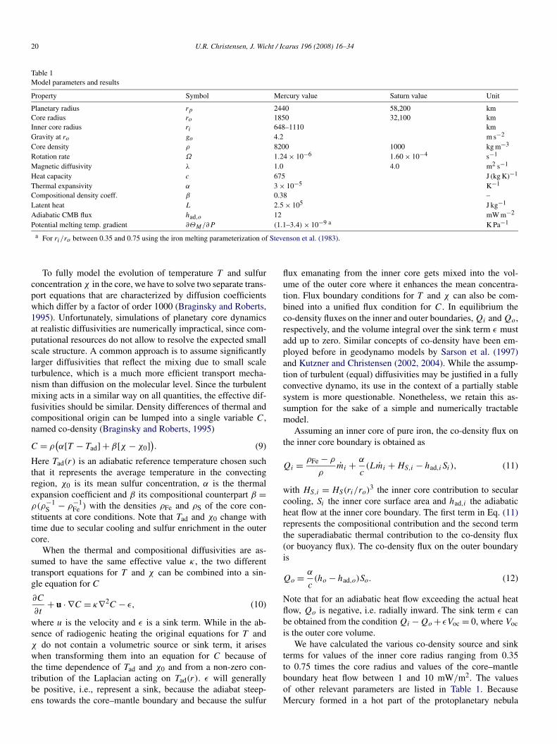
Fig. 1. (a) Inner boundary co-density flux for sulfur contents of 0.3% (gray)and 3% (black). ri/ro is 0.35 (solid lines), 0.50 (dotted), and 0.75 (dashed).(b) Relative thickness of unstable region.

close to the Sun and sulfur is a volatile element, its abun-dance is usually assumed to be less than in other terrestrialplanets (Lewis, 1988). However, Mercury may have been ac-creted partly from planetesimals that formed at larger distancefrom the Sun (Wetherill, 1988), so that the sulfur content of itscore is difficult to estimate. Here we consider sulfur concen-trations in the outer core of 0.3 and 3% by mass. To obtain arough estimate of the thickness of the unstable layer, we solvea simple stationary radial diffusion equation for co-density atgiven values of Qi , Qo and ε. When Qo < 0 the solutionhas a minimum at radius rn (ri < rn < ro), which we call theneutral radius. The relative thickness of the unstable region isdn = (rn − ri)/(ro − ri).

Fig. 1 shows the co-density flux at the inner core bound-ary and the relative thickness of the unstable layer for therange of parameters considered here. The buoyancy flux canbecome negative for an inner core radius of 0.75ro and smallheat flow values, which means that no power remains to drivethe dynamo. These parameter combinations can thus be ex-cluded for Mercury, assuming that it has an active dynamo.For CMB heat flow values of 2–5 mW/m2, which is perhapsthe most likely range according to the thermal evolution mod-els, Qi is in the range of 2000 to 10,000 kg/s for an innercore that is not too big. The relative thickness of the con-vecting layer is approximately between 25 and 60% of theouter core thickness in this case. These estimates will guideus in selecting the parameters for our different dynamo mod-els.

3. Dynamo model setup

3.1. Basic equations and boundary conditions

We study convection and magnetic field generation in a ro-tating spherical shell with inner radius ri and outer radius ro.We vary the ratio η = ri/ro between 0.35 and 0.60. In the restof the paper we use scaled variables. Length is scaled by theshell thickness D = ro − ri , time t by D2/λ, where λ = (μσ)−1

is the magnetic diffusivity, and co-density C by qiD/κ , whereqi is the co-density flux per unit area imposed at ri and κ is itsdiffusivity. Magnetic induction B is scaled by (ρμλΩ)1/2. Wesolve the following set of equations:

E

Pm

(∂u∂t

+ u · ∇u)

+ 2z × u + ∇Π

(13)= E∇2u + RaEPm

Pr

rro

C + (∇ × B) × B,

(14)∂B∂t

− ∇ × (u × B) = ∇2B,

(15)∂C

∂t+ u · ∇C = Pm

Pr∇2C − ε,

(16)∇ · u = 0, ∇ · B = 0.

Here the unit vector z indicates the direction of the rotation axis,Π is dynamic pressure, and gravity varies linearly with radius r .The non-dimensional control parameters are the Ekman number

(17)E = ν

ΩD2,

where ν is the kinematic viscosity, the Prandtl number

(18)Pr = ν

κ,

the magnetic Prandtl number

(19)Pm = ν

λ,

and the Rayleigh number

(20)Ra = goqiD4

κ2νρ,

which is based on the co-density flux at the inner boundary. Thecombination E/Pm is also called the magnetic Ekman number.

We impose a co-density flux boundary condition at ri , i.e.,in non-dimensional terms ∂C/∂r = −1. At ro we set C = 0.The latter condition is taken for simplicity; a flux condition onthe outer boundary may be more realistic for dynamos in ter-restrial planets. However, on time average the flux on the outerboundary will be in balance with the flux at ri and the volumet-ric sink ε once the system has equilibrated. We are interested incases where the flux at ro is negative (inward). As discussed inSection 2 we use the minimum in the diffusive solution to theco-density equation to define the neutral radius rn and the nom-inal thickness dn of the unstable layer. The non-dimensionalvalue of the sink term ε required to obtain a given value of rn iscalculated as

(21)ε = 3η2(1 − η)

3 3 3.

rn(1 − η) − η

22 U.R. Christensen, J. Wicht / Icarus 196 (2008) 16–34

We point out that with our formulation of the problem we donot strictly impose a fixed boundary for the stable layer. In theconvective state the actual thickness of the unstable layer, inthe sense of distance of the minimum of the horizontal average[C](r) above the inner core boundary, may differ from dn.

We assume impenetrable no-slip boundaries in most cases,i.e., u = 0 at ri and ro. In a few cases we use free slip on theouter boundary, for reasons explained below. The magnetic fieldat ro is matched continuously with a potential field lacking ex-ternal sources. The inner core is assumed to co-rotate with theouter boundary (the mantle) when we use no-slip conditions. Inthe case of free slip at ro the inner core rotation rate relativeto the reference frame is controlled by viscous and magnetictorques. The inner core is assumed to have the same electri-cal conductivity as the fluid shell in all cases except one, andat r < ri we solve the induction equation (14) with u = 0 (orwith the velocity field of solid body rotation where applicable),subject to the appropriate continuity conditions at ri .

For numerical treatment we express the velocity and mag-netic field in terms of poloidal and toroidal scalars and expandthese and the co-density in spherical harmonic functions up todegree and order �max in the angular variables θ and φ and inChebychev polynomials up to degree Nr in the radial direc-tion. A spectral transform method, which is described in somedetail in Christensen and Wicht (2007), is then used to solveEqs. (13)–(15). We found that in order to avoid spurious struc-tures in the (very weak) poloidal magnetic field at the outerboundary we need a higher number of radial modes than onewould normally use in dynamo calculations at similar parame-ter values.

Some simulations have been started from a diffusive solutionwith weak perturbations, but in most cases we used the finalstate of another simulation as starting condition. The run timewas usually one magnetic diffusion time τD = r2

o /λ based onthe radius of the whole sphere. Some cases ran for a shortertime, but at least for τD/2. All cases appear to have reached anequilibrated state.

3.2. Choice of model parameters

It is well-known that planetary dynamo models cannot becalculated at realistic values of all model parameters. In par-ticular, in order to suppress small-scale eddies in the flow thatare unresolvable with current numerical means, far too largevalues must be used for the viscosity and the thermal and com-positional diffusivities. In terms of non-dimensional numbers,the Ekman number and the magnetic Prandtl number are muchlarger than they are in planetary cores and the Rayleigh numberis smaller. However, arguably the most important parameter fora dynamo is the magnetic Reynolds number

(22)Rm = urmsD

λ.

Even though the individual values of Ra, E and Pm cannot bechosen such that they match planetary values, we can aim atusing a combination of these parameters that lead to appropriatevalues of Rm in the models.

Christensen and Aubert (2006) and Olson and Christensen(2006) derived from systematic dynamo model studies scalinglaws that relate the characteristic flow velocity to a modifiedRayleigh number. Using their results, we obtain the dependenceof the magnetic Reynolds number on the control parametersemployed here as

(23)Rm = aPm(ηRa)2/5E1/5Pr−4/5,

where a is a numerical constant. Cast into physical propertiesthis gives

(24)Rm = a

(η2g2

oq2i D6

λ5ρ2Ω

)1/5

.

Christensen and Aubert (2006) found a = 0.85 for dynamoswith η = 0.35 in which the whole spherical shell is convecting.When convection is restricted to a sublayer of thickness dn, a isexpected to be smaller and to depend on dn and η. Our simula-tions suggest that a ranges between 0.4–0.5 when dn is around0.4.

Taking the parameter values for Mercury from Table 1,η = 0.5 and a co-density flux Qi = 4πr2

i qi between 2000 and10,000 kg s−1, Eq. (24) predicts values of Rm in the range of400–800 when a = 0.4. This is approximately half of the valueestimated for the Earth’s core applying the same scaling rela-tions (Christensen and Aubert, 2006) and certainly high enoughfor a self-sustained dynamo. We note that we use the full shellthickness D in the definition of the magnetic Reynolds number(Eq. (22)). Taking the thickness dn of the convective sublayermay be more appropriate, which reduces the effective value ofRm. This is partly balanced by employing in Eq. (22) the rms-value of velocity taken over the entire shell, which is smallerthan the mean in the unstable sublayer.

Aside from matching the planetary value of the magneticReynolds number in the numerical models, we strive to makesure that the dynamo falls into the regime, dipolar or multipo-lar, that is appropriate for the planet under consideration. Asmentioned before, the dynamo regime is primarily controlledby the value of the local Rossby number (Eq. (4)). Olson andChristensen (2006) found the following scaling laws for the lo-cal Rossby number in terms of non-dimensional parameters

(25)Ro� = a′Ra1/2E7/6Pr−4/5Pm−1/5

and in terms of physical properties

(26)Ro� = a′(

goqi

ρ

)1/2

Ω−7/6(Dν)−1/3(

λ

κ

)1/5

,

where the prefactor a′ is of order one. They estimated for Mer-cury Ro� = O(10) and for Saturn Ro� = O(10−2). The thresh-old for the transition from dipolar to multipolar dynamos isRo� = 0.12 in case of fully convective dynamos with no-slipboundaries and driven from below. The transitional value de-pends on the mode of driving of the dynamo (Olson and Chris-tensen, 2006) and is sensitive to details of its geometry, but willprobably not deviate from 0.1 by more than an order of magni-tude. Hence Saturns dynamo should fall into the dipolar regime,whereas Mercury’s dynamo is expected to be multipolar.

Magnetic field generation in Mercury and Saturn 23

A caveat against the criterion of the local Rossby number isthat the flow length scale � (Eq. (4)), which is of the order 100 mat the quoted value of Ro�, is too small to affect in a direct waythe magnetic field. At this scale the field is diffusion-dominated.However, in rotational flow an inverse cascade transports ki-netic energy from small scales to scales that are large enoughto play a role magnetic field generation. Hence the small flowscales may affect the magnetic field in an indirect way. Whilethe merits of the local Rossby number rule still need furthertesting, its relevance at planetary conditions is supported by thefinding that it seems to apply for dynamos at values of the mag-netic Prandtl number both larger than one and smaller than one,i.e., in situations where the magnetic length scale is smaller orwhere it is larger then the flow length scale (Christensen andAubert, 2006).

Equation (25) indicates that in numerical dynamo models forMercury the Ekman number should not be too low, whereas theRayleigh number must be large in order to reach a value of Ro�

that puts the dynamo into the multipolar regime. This is in con-flict with the desire for a low model value of E (whose planetaryvalue is as low as 10−12 even in slowly rotating Mercury). Theexpected Mercury value of Ro� cannot be reached without com-promising severely on the value of the Ekman number, with thepossible consequence that viscous effects, which are thought tobe unimportant in planetary dynamos, dominate the dynamicsin the model. Christensen and Aubert (2006) found that viscos-ity does not seem to play a big role in dynamo models whenE � 3 × 10−4. Therefore, we took in most of our models theEkman number to be either 10−4 or 3 × 10−5 and varied theRayleigh number inbetween 2 × 108 and 8 × 108. Most of thedynamos fall into the multipolar regime. A value of one is takenfor the Prandtl number. A magnetic Prandtl number of threeto five puts the magnetic Reynolds number into the range thatwe estimated for Mercury. The magnetic Reynolds number inSaturn, which is of the order 104 (Stevenson, 2003), cannot bereached in numerical dynamo simulations.

4. Results

We have calculated 20 model simulations, whose parametersand results are summarized in Table 2. We monitored severalmodel properties and list their time-average values. The Nus-selt number, as a measure of the relative efficiency of advectivetransport of co-density in the convecting region, is defined as

(27)Nu = Cd(ri) − Cd(rn)

[C](ri) − [C]min,

where Cd refers to the diffusive solution of Eq. (15) and [C] tothe horizontal and time average in the convective state. [C]min

is the minimum of [C](r). The Nusselt number is inbetweentwo and seven in our models, indicating that convection in theunstable layer is well above the critical point of onset. The El-sasser number Λ represents the strength of the magnetic field inthe dynamo region and has been calculated with its rms-valuein the region ri < r < rn. The values range in between 1 and 10in most models, i.e., the internal dynamo field is strong.

Ta

ble

2M

odel

para

met

ers

and

resu

lts

Mod

el1

1a1b

22a

34

4a4b

56

78

910

1112

1313

a13

b

Ra/

107

401.

1640

2020

4060

2.29

6080

8040

4060

5025

2025

0.72

525

E/10

−53

17.6

310

1010

1051

.210

33

33

1010

1010

03

17.6

3P

m3

33

33

33

33

33

33

33

33

55

5η

0.35

0.57

0.35

0.5

0.5

0.5

0.5

0.69

0.5

0.35

0.35

0.35

0.35

0.6

0.5

0.35

0.5

0.35

0.57

0.35

BC

01

20

30

01

20

00

00

00

00

12

dn

0.41

10.

410.

440.

440.

440.

441

0.44

0.41

0.30

0.50

0.60

0.35

0.36

0.41

0.44

0.41

10.

41�

max

8585

8510

685

106

106

8510

685

8585

8513

485

6410

664

8564

Nr

8141

8165

4965

6541

6561

8149

4965

6161

6561

4141

t run

1.38

1.01

1.00

1.00

1.10

1.06

1.09

1.00

0.87

1.02

1.02

1.10

1.02

0.53

1.34

1.23

1.00

1.00

0.93

0.64

Rm

291

211

131

348

342

480

591

423

429

324

273

315

261

525

462

357

466

205

211

145

Nu

2.25

2.47

2.48

4.33

4.33

5.70

6.53

6.81

6.47

3.38

2.60

2.59

3.40

6.04

5.30

3.47

5.72

2.19

1.95

2.08

Λ0.

741.

35.

92.

31.

44.

88.

313

9.4

2.1

1.0

0.98

6.8

7.0

4.8

1.4

329.

45.

312

Bs

[nT

]91

1950

4570

890

400

420

285

7400

960

380

5316

020

,400

240

180

230

1190

22,1

0024

,700

30,4

00E

dip

37%

19%

93%

97%

37%

88%

86%

50%

53%

4%48

%25

%97

%92

%85

%10

%2%

>99

%77

%>

99%

Equ

ad35

%33

%3%

1%22

%5%

6%6%

20%

51%

24%

39%

2%1%

6%86

%92

%0%

21%

0%E

oct

20%

25%

0%1%

25%

5%6%

31%

14%

13%

24%

23%

1%6%

9%2%

0%0%

1%0%

Em

>0

39%

87%

1%1%

41%

3%3%

96%

78%

4%5%

28%

2%5%

3%5%

1%0%

24%

0%N

rev

2433

00

016

49

460

1745

1733

00

68

00

50

Cod

efo

rbo

unda

ryco

nditi

on(B

C):

0—st

anda

rd,1

—fr

eesl

ipat

r=

r o,2

—st

able

laye

rim

mob

ilize

d,3—

insu

latin

gin

ner

core

.The

surf

ace

mag

netic

field

stre

ngth

has

been

scal

edus

ing

Mer

cury

para

met

ers,

exce

ptin

case

s8,

13,1

3aan

d13

b,w

here

Satu

rnpa

ram

eter

sha

vebe

enus

ed.

24 U.R. Christensen, J. Wicht / Icarus 196 (2008) 16–34

Other values in Table 2 refer to the magnetic field upwardcontinued from ro to the planetary surface and scaled to plane-tary values. In most cases this has been done using the Mercuryproperties of Table 1, except for a few cases in the dipolar dy-namo regime, where Saturn parameters have been taken. Bs isthe mean surface field strength in harmonic modes n = 1 ton = 8. Edip, Equad and Eoct are the contributions of magneticenergy at harmonic degree n equal to one, two, three, respec-tively, relative to the energy of the surface field in degrees one toeight. Em>0 is the relative energy in non-axisymmetric modes.Nrev is the number of reversals during one magnetic diffusiontime τD of the full sphere, which is 108,500 yr for our adoptedMercury parameters. Each change of sign of the Gauss coeffi-cient g0

1 has been counted as a reversal. However, in those caseswhere Equad > Edip the coefficient g0

2 has been taken instead.Model cases 1 and 2, with a ratio η = ri/ro of 0.35 and 0.5,

respectively, have been discussed in Christensen (2006). Thesurface field strength is one fifth of the observed strength atMercury in case 1 and twice the observed strength in case 2.In case 1, the dipole and the quadrupole contribute on time-average equally to the surface field and reverse on a time scaleof 5000 yr, whereas in case 2 the surface field is strongly dom-inated by the axial dipole, which did not reverse during themodel run time.

4.1. Models fitting Mercury’s field

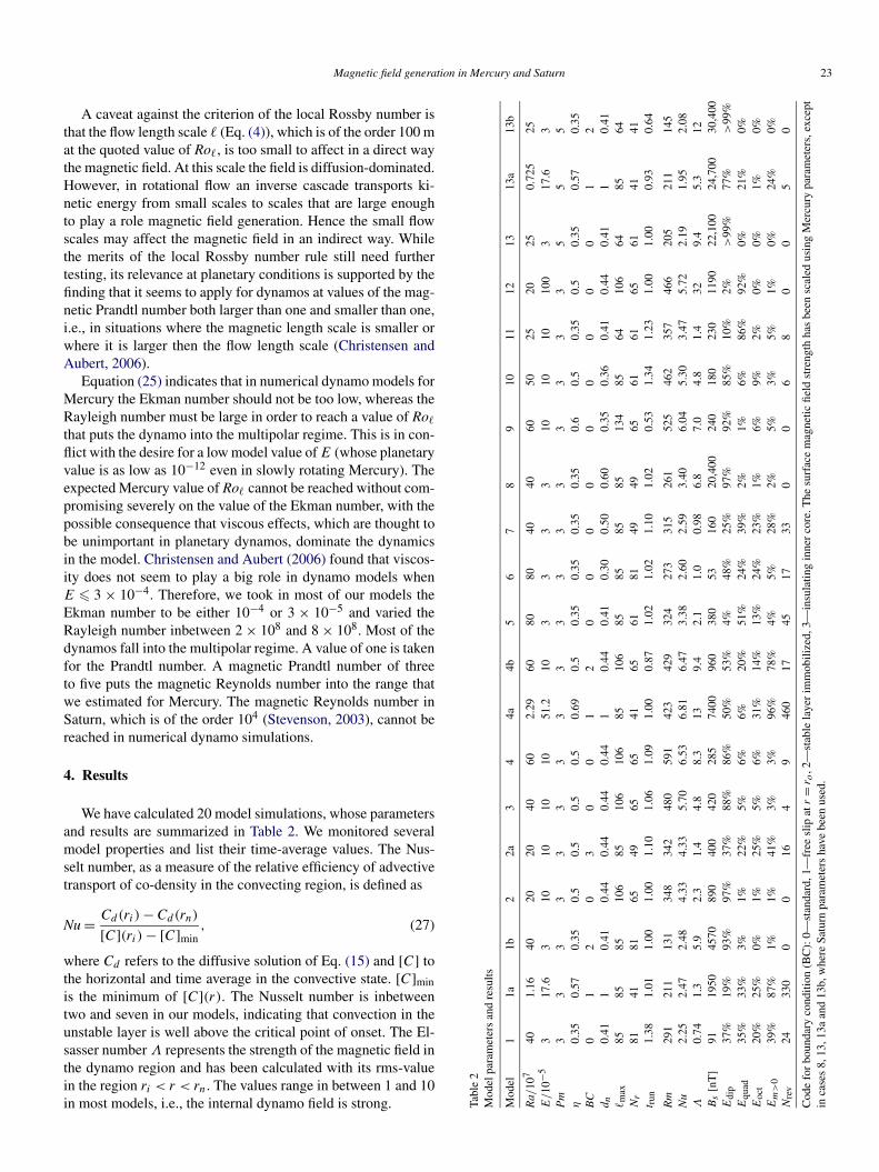
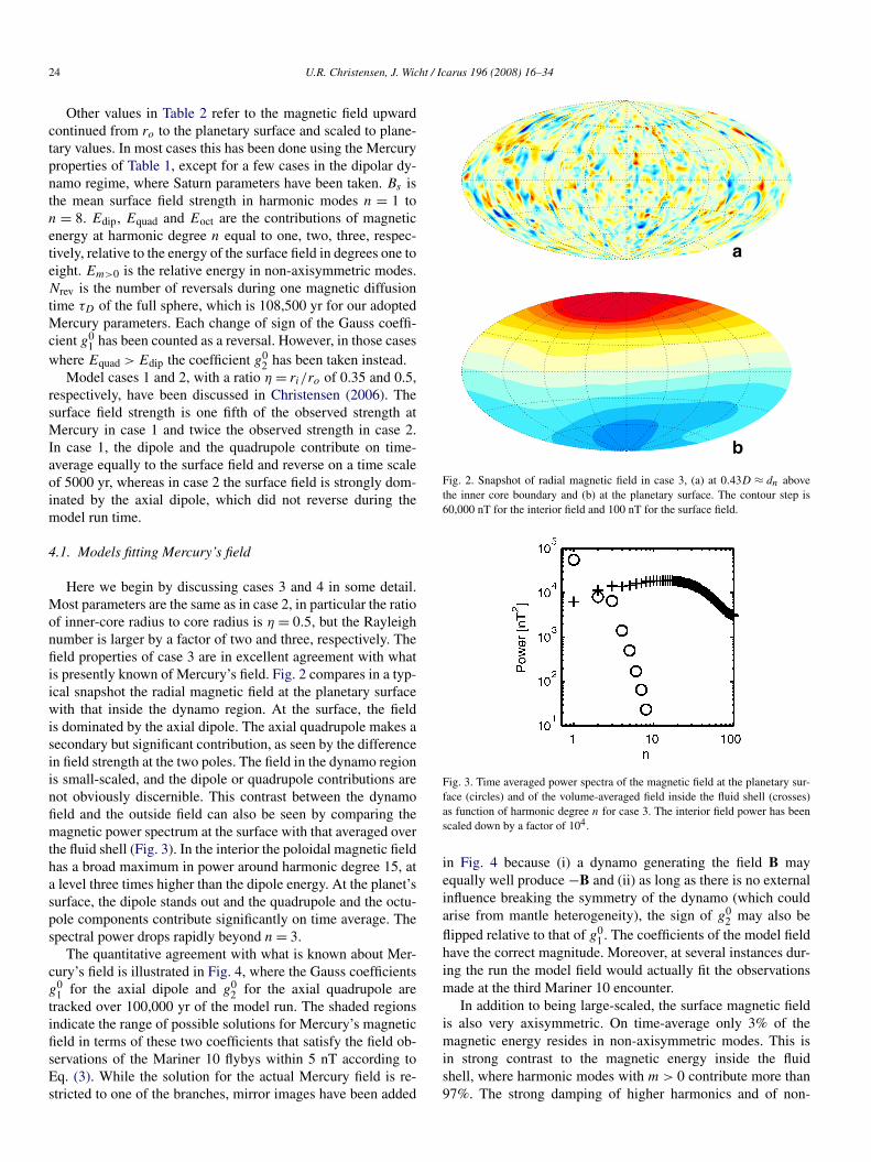
Here we begin by discussing cases 3 and 4 in some detail.Most parameters are the same as in case 2, in particular the ratioof inner-core radius to core radius is η = 0.5, but the Rayleighnumber is larger by a factor of two and three, respectively. Thefield properties of case 3 are in excellent agreement with whatis presently known of Mercury’s field. Fig. 2 compares in a typ-ical snapshot the radial magnetic field at the planetary surfacewith that inside the dynamo region. At the surface, the fieldis dominated by the axial dipole. The axial quadrupole makes asecondary but significant contribution, as seen by the differencein field strength at the two poles. The field in the dynamo regionis small-scaled, and the dipole or quadrupole contributions arenot obviously discernible. This contrast between the dynamofield and the outside field can also be seen by comparing themagnetic power spectrum at the surface with that averaged overthe fluid shell (Fig. 3). In the interior the poloidal magnetic fieldhas a broad maximum in power around harmonic degree 15, ata level three times higher than the dipole energy. At the planet’ssurface, the dipole stands out and the quadrupole and the octu-pole components contribute significantly on time average. Thespectral power drops rapidly beyond n = 3.

The quantitative agreement with what is known about Mer-cury’s field is illustrated in Fig. 4, where the Gauss coefficientsg0

1 for the axial dipole and g02 for the axial quadrupole are

tracked over 100,000 yr of the model run. The shaded regionsindicate the range of possible solutions for Mercury’s magneticfield in terms of these two coefficients that satisfy the field ob-servations of the Mariner 10 flybys within 5 nT according toEq. (3). While the solution for the actual Mercury field is re-stricted to one of the branches, mirror images have been added

Fig. 2. Snapshot of radial magnetic field in case 3, (a) at 0.43D ≈ dn abovethe inner core boundary and (b) at the planetary surface. The contour step is60,000 nT for the interior field and 100 nT for the surface field.

Fig. 3. Time averaged power spectra of the magnetic field at the planetary sur-face (circles) and of the volume-averaged field inside the fluid shell (crosses)as function of harmonic degree n for case 3. The interior field power has beenscaled down by a factor of 104.

in Fig. 4 because (i) a dynamo generating the field B mayequally well produce −B and (ii) as long as there is no externalinfluence breaking the symmetry of the dynamo (which couldarise from mantle heterogeneity), the sign of g0

2 may also beflipped relative to that of g0

1 . The coefficients of the model fieldhave the correct magnitude. Moreover, at several instances dur-ing the run the model field would actually fit the observationsmade at the third Mariner 10 encounter.

In addition to being large-scaled, the surface magnetic fieldis also very axisymmetric. On time-average only 3% of themagnetic energy resides in non-axisymmetric modes. This isin strong contrast to the magnetic energy inside the fluidshell, where harmonic modes with m > 0 contribute more than97%. The strong damping of higher harmonics and of non-

Magnetic field generation in Mercury and Saturn 25

axisymmetric modes in the field outside the core has been ex-plained in Christensen (2006) by the different time-dependentbehavior of the various modes generated in the dynamo region.All field components show fast fluctuations on time-scales of200 yr (Fig. 5). These are almost completely filtered out by theskin effect when the field diffuses through the stably stratified

Fig. 4. Plot of Gauss coefficient g01 versus g0

2 during the model run of case 3.Shaded regions indicate acceptable models for Mercury’s actual field as de-scribed in the text.

layer (which we will treat for the moment as if it were com-pletely stagnant). However, the low-order axisymmetric modes,such as the axial dipole, have a component that varies with longperiods up to 100,000 yr. These low-frequency components canescape through the stable layer with little or no attenuation,aside from the geometric decrease of the field strength accord-ing to r−(n+2). The non-axisymmetric modes have very littleenergy at low frequencies and are largely lost in the outsidefield (Fig. 5b). The relative power at low frequencies tendsto become less with increasing harmonic degree also for theaxisymmetric modes (Fig. 5c). This agrees with the findingfrom observations of the geomagnetic field (Olsen et al., 2006)and geodynamo modeling (Christensen and Tilgner, 2004) thatthe characteristic time scale of secular variation depends onharmonic degree as n−1 or n−1.35. Higher harmonics are sup-pressed compared to low-order components in the outside fieldnot only by their faster geometric decay, but also by a strongerskin effect. Christensen and Tilgner (2004) found that, asidefrom the dependence on n, the secular variation time scale iscontrolled by the magnetic Reynolds number. Since the modelvalues of Rm are arguably in the correct range for Mercury, thefiltering by the skin effect should be correctly represented in themodels.

For fluctuations of intermediate periods, T ≈ 5000 yr, aphase lag of the outside field relative to the interior field ofabout 1500 yr is obvious in Fig. 5d. This compares well withthe predicted phase lag for the diffusion through a plane layerof thickness D/2, which is T D/(2

√4πλT ) ≈ 1600 yr.

The Rayleigh number is increased stepwise going fromcase 2 to case 4 for otherwise identical parameters. The mag-netic field strength in the dynamo region increases with theRayleigh number; the Elsasser number Λ rises from 2.3 to

Fig. 5. Time series of Gauss coefficients (full line) for case 3. The gray line shows an equivalent coefficient describing the poloidal magnetic field at r = ri + D/2inside the fluid shell, scaled down by 0.1. (a) Axial dipole, (b) equatorial dipole component, (c) axial quadrupole, (d) closeup for the axial dipole.

26 U.R. Christensen, J. Wicht / Icarus 196 (2008) 16–34

8.3. However, the time-average surface magnetic field becomesweaker, from an rms-value of 890 nT in case 2, to 420 nT incase 3, and to 285 nT in case 4. Compared to Mercury fieldmodels based on Mariner 10 data, the last value is slightly onthe low side, but at some instances in time the combination ofaxial dipole and axial quadrupole moments falls into the rangegiven by Eq. (3) also in model 4. The reason for the oppositetrends of the internal and the surface field strength is that withincreasing Rayleigh number relatively less magnetic energy iscarried by the low-degree modes, and they tend to fluctuateat shorter periods. For example, the axial dipole shows no re-versals in case 2, four reversals per magnetic diffusion time incase 3, and nine reversals in case 4.

An interesting question is why only the axisymmetric modesin the dynamo field have a low-frequency component that canpass the stable layer, whereas non-axisymmetric modes at thesame harmonic degree do not. A fundamental reason for thepreference for axisymmetric modes is the structuring of the flowby the Coriolis force, which tends to create a statistical align-ment with the rotation axis. There is no preferred longitude(barring coupling of the dynamo to a heterogeneous exteriorstructure), and non-axisymmetric modes should be able to driftfreely in longitude. For the axisymmetric modes both polari-ties are possible in principle, and in some dynamo models witha weak relative dipole contribution the dipole reverses errati-cally on short time scales (Kutzner and Christensen, 2002). Inthe present models the dipole polarity is stabilized by the stag-nant conducting regions of the solid inner core. For η = 0.5 thedipole decay time of the inner core r2

i /(π2λ) is 2700 yr. It isexpected that statistical polarity fluctuations in the fluid coreonly lead to a complete reversal if they persist for a longer time(Hollerbach and Jones, 1993), thus stabilizing a given polar-ity. We tested this hypothesis by branching off from the non-reversing case 2 a simulation where the inner core conductivityis set to zero (case 2a). After a transitional period it settled intoa state with frequent dipole reversals. As a consequence, thesurface magnetic field is significantly weaker than in case 2 andthe axial dipole is no longer as dominant as before (Table 2).In similar tests for geodynamo-like models Wicht (2002) foundlittle evidence for a stabilizing effect of inner core conductivity.The relatively larger size of the inner core and the additionalstabilizing influence of the stably stratified conducting layer inthe fluid shell may provide sufficient magnetic inertia to makethe effect significant in the present models.

While inner core conductivity can explain the relative stabil-ity of the axial dipole polarity even in a dynamo whose dipolefield is weak compared to higher multipole components, it canbe argued that the same effect could likewise stabilize the equa-torial dipole against rapid variations. This does not happen inour models. In order to understand the reasons, we must con-sider the flow in the stably stratified layer and its effect on themagnetic field.

4.2. Flow in the stable layer

Fig. 6 shows the variation of velocity and magnetic field withradius. In the dynamo region, poloidal and toroidal velocity

Fig. 6. Variation of components of the velocity (a) and of the magnetic field(b) with radius in case 4. rms-values averaged in the angular directions andin time are shown. Full line—poloidal component, broken line—toroidal, dot-ted—axisymmetric toroidal, dash-dotted—axisymmetric poloidal. The axisym-metric poloidal velocity is tiny and not shown. The vertical line indicates thenominal radius of neutral stability.

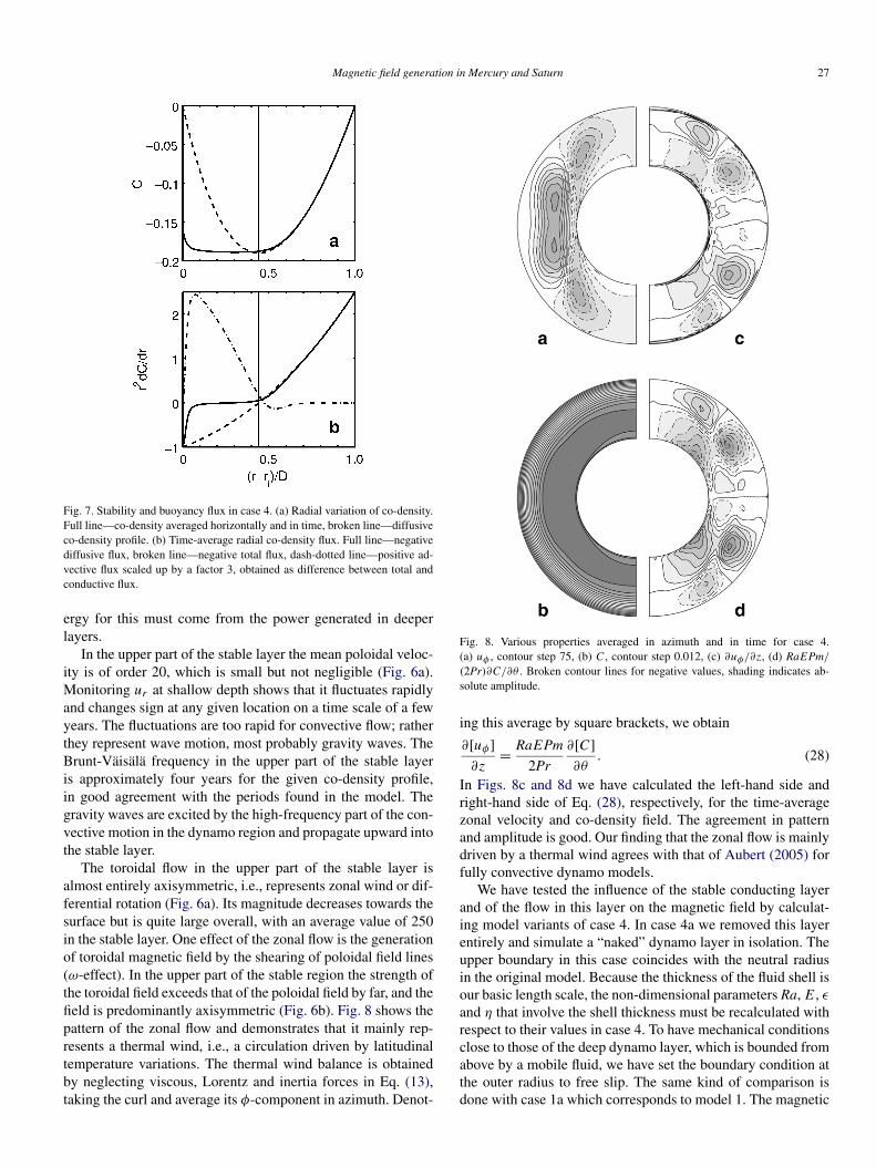
components have similar amplitude, as expected for columnarconvection. In the stable layer the flow is mainly toroidal andweaker than in the convecting region, but not much weaker. Ina transitional region that extends roughly to 0.65D above theinner core boundary, overshooting of convection is the maincontributor to the poloidal and the non-axisymmetric toroidalvelocity. As shown in Christensen (2006), convection columnsthat align with the rotation axis penetrate into the stable layer,although the velocity decreases in magnitude and becomes in-creasingly toroidal with distance from the equatorial plane. Thisis akin to “teleconvection” described by Zhang and Schubert(2000). In the convective state the thickness of the unstablelayer, in the sense of the distance of the minimum in the radi-ally averaged co-density profile from the inner core boundary(Fig. 7a) is less than the nominal thickness dn based on theminimum in the diffusive profile (0.32 versus 0.441, respec-tively). However, the radius at which the advective co-densityflux (buoyancy flux) reaches zero is almost identical to the nom-inal value of the neutral radius (Fig. 7b). In the overshoot regionsome downward advection of co-density occurs in addition tothe downward diffusive flux. This enables mixing in this regionand implies that work is done against buoyancy forces. The en-

Magnetic field generation in Mercury and Saturn 27

Fig. 7. Stability and buoyancy flux in case 4. (a) Radial variation of co-density.Full line—co-density averaged horizontally and in time, broken line—diffusiveco-density profile. (b) Time-average radial co-density flux. Full line—negativediffusive flux, broken line—negative total flux, dash-dotted line—positive ad-vective flux scaled up by a factor 3, obtained as difference between total andconductive flux.

ergy for this must come from the power generated in deeperlayers.

In the upper part of the stable layer the mean poloidal veloc-ity is of order 20, which is small but not negligible (Fig. 6a).Monitoring ur at shallow depth shows that it fluctuates rapidlyand changes sign at any given location on a time scale of a fewyears. The fluctuations are too rapid for convective flow; ratherthey represent wave motion, most probably gravity waves. TheBrunt-Väisälä frequency in the upper part of the stable layeris approximately four years for the given co-density profile,in good agreement with the periods found in the model. Thegravity waves are excited by the high-frequency part of the con-vective motion in the dynamo region and propagate upward intothe stable layer.

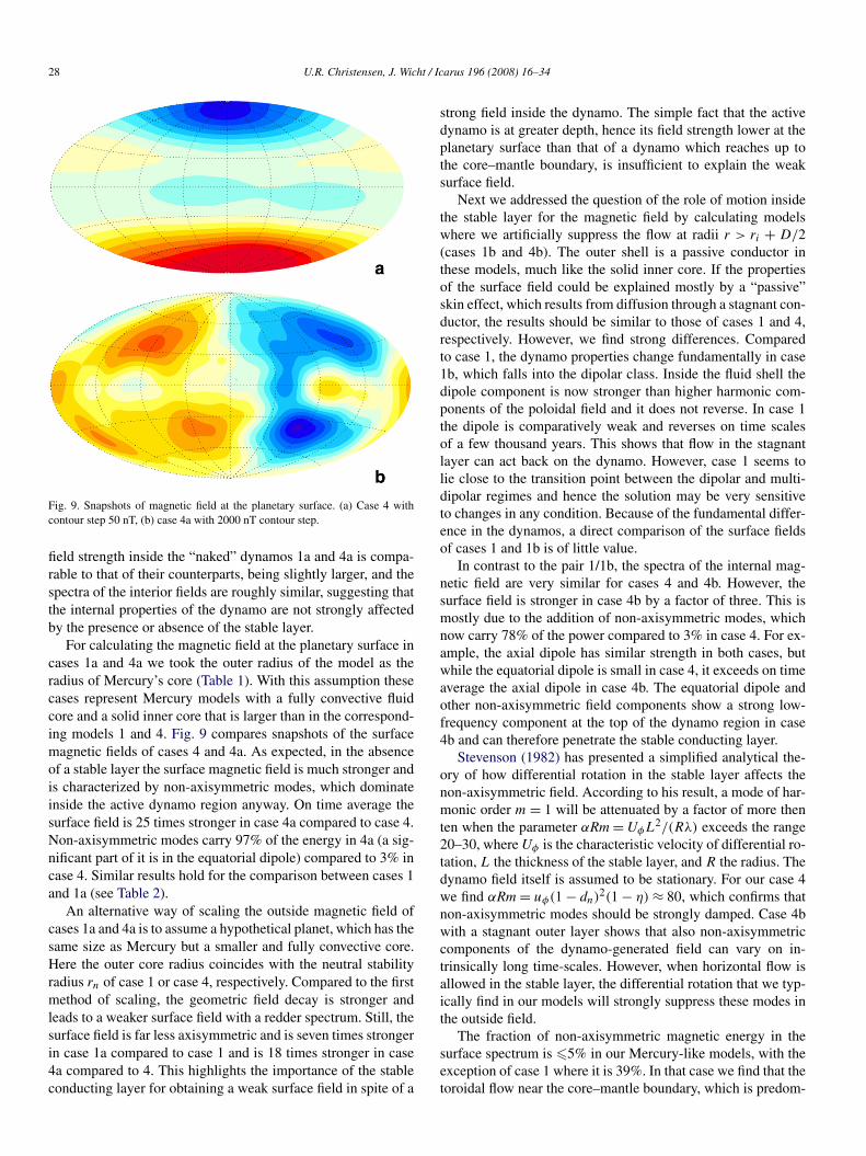
The toroidal flow in the upper part of the stable layer isalmost entirely axisymmetric, i.e., represents zonal wind or dif-ferential rotation (Fig. 6a). Its magnitude decreases towards thesurface but is quite large overall, with an average value of 250in the stable layer. One effect of the zonal flow is the generationof toroidal magnetic field by the shearing of poloidal field lines(ω-effect). In the upper part of the stable region the strength ofthe toroidal field exceeds that of the poloidal field by far, and thefield is predominantly axisymmetric (Fig. 6b). Fig. 8 shows thepattern of the zonal flow and demonstrates that it mainly rep-resents a thermal wind, i.e., a circulation driven by latitudinaltemperature variations. The thermal wind balance is obtainedby neglecting viscous, Lorentz and inertia forces in Eq. (13),taking the curl and average its φ-component in azimuth. Denot-

Fig. 8. Various properties averaged in azimuth and in time for case 4.(a) uφ , contour step 75, (b) C, contour step 0.012, (c) ∂uφ/∂z, (d) RaEPm/

(2Pr)∂C/∂θ . Broken contour lines for negative values, shading indicates ab-solute amplitude.

ing this average by square brackets, we obtain

(28)∂[uφ]∂z

= RaEPm

2Pr

∂[C]∂θ

.

In Figs. 8c and 8d we have calculated the left-hand side andright-hand side of Eq. (28), respectively, for the time-averagezonal velocity and co-density field. The agreement in patternand amplitude is good. Our finding that the zonal flow is mainlydriven by a thermal wind agrees with that of Aubert (2005) forfully convective dynamo models.

We have tested the influence of the stable conducting layerand of the flow in this layer on the magnetic field by calculat-ing model variants of case 4. In case 4a we removed this layerentirely and simulate a “naked” dynamo layer in isolation. Theupper boundary in this case coincides with the neutral radiusin the original model. Because the thickness of the fluid shell isour basic length scale, the non-dimensional parameters Ra, E, εand η that involve the shell thickness must be recalculated withrespect to their values in case 4. To have mechanical conditionsclose to those of the deep dynamo layer, which is bounded fromabove by a mobile fluid, we have set the boundary condition atthe outer radius to free slip. The same kind of comparison isdone with case 1a which corresponds to model 1. The magnetic

28 U.R. Christensen, J. Wicht / Icarus 196 (2008) 16–34

Fig. 9. Snapshots of magnetic field at the planetary surface. (a) Case 4 withcontour step 50 nT, (b) case 4a with 2000 nT contour step.

field strength inside the “naked” dynamos 1a and 4a is compa-rable to that of their counterparts, being slightly larger, and thespectra of the interior fields are roughly similar, suggesting thatthe internal properties of the dynamo are not strongly affectedby the presence or absence of the stable layer.

For calculating the magnetic field at the planetary surface incases 1a and 4a we took the outer radius of the model as theradius of Mercury’s core (Table 1). With this assumption thesecases represent Mercury models with a fully convective fluidcore and a solid inner core that is larger than in the correspond-ing models 1 and 4. Fig. 9 compares snapshots of the surfacemagnetic fields of cases 4 and 4a. As expected, in the absenceof a stable layer the surface magnetic field is much stronger andis characterized by non-axisymmetric modes, which dominateinside the active dynamo region anyway. On time average thesurface field is 25 times stronger in case 4a compared to case 4.Non-axisymmetric modes carry 97% of the energy in 4a (a sig-nificant part of it is in the equatorial dipole) compared to 3% incase 4. Similar results hold for the comparison between cases 1and 1a (see Table 2).

An alternative way of scaling the outside magnetic field ofcases 1a and 4a is to assume a hypothetical planet, which has thesame size as Mercury but a smaller and fully convective core.Here the outer core radius coincides with the neutral stabilityradius rn of case 1 or case 4, respectively. Compared to the firstmethod of scaling, the geometric field decay is stronger andleads to a weaker surface field with a redder spectrum. Still, thesurface field is far less axisymmetric and is seven times strongerin case 1a compared to case 1 and is 18 times stronger in case4a compared to 4. This highlights the importance of the stableconducting layer for obtaining a weak surface field in spite of a

strong field inside the dynamo. The simple fact that the activedynamo is at greater depth, hence its field strength lower at theplanetary surface than that of a dynamo which reaches up tothe core–mantle boundary, is insufficient to explain the weaksurface field.

Next we addressed the question of the role of motion insidethe stable layer for the magnetic field by calculating modelswhere we artificially suppress the flow at radii r > ri + D/2(cases 1b and 4b). The outer shell is a passive conductor inthese models, much like the solid inner core. If the propertiesof the surface field could be explained mostly by a “passive”skin effect, which results from diffusion through a stagnant con-ductor, the results should be similar to those of cases 1 and 4,respectively. However, we find strong differences. Comparedto case 1, the dynamo properties change fundamentally in case1b, which falls into the dipolar class. Inside the fluid shell thedipole component is now stronger than higher harmonic com-ponents of the poloidal field and it does not reverse. In case 1the dipole is comparatively weak and reverses on time scalesof a few thousand years. This shows that flow in the stagnantlayer can act back on the dynamo. However, case 1 seems tolie close to the transition point between the dipolar and multi-dipolar regimes and hence the solution may be very sensitiveto changes in any condition. Because of the fundamental differ-ence in the dynamos, a direct comparison of the surface fieldsof cases 1 and 1b is of little value.

In contrast to the pair 1/1b, the spectra of the internal mag-netic field are very similar for cases 4 and 4b. However, thesurface field is stronger in case 4b by a factor of three. This ismostly due to the addition of non-axisymmetric modes, whichnow carry 78% of the power compared to 3% in case 4. For ex-ample, the axial dipole has similar strength in both cases, butwhile the equatorial dipole is small in case 4, it exceeds on timeaverage the axial dipole in case 4b. The equatorial dipole andother non-axisymmetric field components show a strong low-frequency component at the top of the dynamo region in case4b and can therefore penetrate the stable conducting layer.

Stevenson (1982) has presented a simplified analytical the-ory of how differential rotation in the stable layer affects thenon-axisymmetric field. According to his result, a mode of har-monic order m = 1 will be attenuated by a factor of more thenten when the parameter αRm = UφL2/(Rλ) exceeds the range20–30, where Uφ is the characteristic velocity of differential ro-tation, L the thickness of the stable layer, and R the radius. Thedynamo field itself is assumed to be stationary. For our case 4we find αRm = uφ(1 − dn)

2(1 − η) ≈ 80, which confirms thatnon-axisymmetric modes should be strongly damped. Case 4bwith a stagnant outer layer shows that also non-axisymmetriccomponents of the dynamo-generated field can vary on in-trinsically long time-scales. However, when horizontal flow isallowed in the stable layer, the differential rotation that we typ-ically find in our models will strongly suppress these modes inthe outside field.

The fraction of non-axisymmetric magnetic energy in thesurface spectrum is �5% in our Mercury-like models, with theexception of case 1 where it is 39%. In that case we find that thetoroidal flow near the core–mantle boundary, which is predom-

Magnetic field generation in Mercury and Saturn 29

Fig. 10. Snapshot of the radial magnetic field at the planetary surface of case 5.Contour interval is 100 nT.

inantly zonal in other models, has a large non-zonal componentrepresenting the penetration of columnar flow far into the sta-ble region (Christensen, 2006). Advection of the dipole field inlatitudinal direction near the core surface modulates the fieldstructure such that it deviates from axisymmetry.

4.3. Variation of inner core radius and stable layer thickness

We have varied the fractional radius η of the inner core be-tween 0.35 and 0.6 and the relative thickness of the unstablelayer between 0.3 and 0.6. The surface magnetic field in thedynamos with η � 0.5 is dominated by the axial dipole (ex-cluding cases without a stable layer). With a small inner core,η = 0.35, we find a tendency towards a strong contribution, oreven dominance, of the axial quadrupole. In case 1, the quadru-pole and dipole contribute equally on time average, with onecomponent dominating at some times and the other compo-nent at other times. In case 5 we doubled the Rayleigh num-ber compared to case 1. This makes the surface magnetic fieldstrongly quadrupolar (Fig. 10). The time average mean surfacefield strength is 380 nT, in agreement with the Mariner 10 ob-servations. In addition to the axial quadrupole, the harmoniccomponent (n,m) = (4,0) is rather large, corresponding to aconcentration of magnetic flux into the two polar caps. Thequadrupolar field reverses nearly periodically on a 5000 yr timescale (Fig. 11). The g0

4 coefficient changes in phase with g02 .

When we reduce the relative thickness of the unstable layerfrom 0.41 in case 5 to 0.30 in case 6, the dominance of the axialdipole is restored, but the quadrupole still makes a significantcontribution. In this case the surface field strength is almost afactor 10 below the Mercury value. Case 7 has the same para-meters as case 1, except that the thickness of the unstable layeris increased from 0.41 to 0.50. At times still the dipole domi-nates, but the axial quadrupole is stronger on average. A furtherincrease of dn to 0.6 (case 8) causes a change from the multi-polar to the dipolar dynamo regime. Case 8 is discussed furtherin Section 4.5.

Obviously the inner core radius cannot be too large for thefiltering effect of the stable layer to be effective, because a verylarge inner core leaves insufficient space for a stable region. Themaximum value of η = 0.6 for which we performed model sim-ulations corresponds to an inner core of 1110 km radius (usingour nominal Mercury properties). At this value of η a model run

Fig. 11. Time series of Gauss coefficients for case 5. See Fig. 5 for explanations.

with parameters similar to those of case 3 led to a dynamo inthe strongly dipolar regime. We found a Mercury-like dynamofor a higher Rayleigh number and smaller value of dn (case 9).The dynamo layer is only 260 km thick in this model. Thedipole-dominated surface magnetic field has a mean strengthof 240 nT.

The main effect of varying the thickness of the unstable layerwith all other parameters held constant is an increase of thesurface field strength with dn (see Table 2). This is quite pre-dictable because both the geometric field decay with r and thefiltering of higher frequencies by the skin effect become weakerfor a thinner stable layer. Furthermore, in most cases there isa trend for the dipole to contribute more strongly to the sur-face field in a relative sense when dn is smaller. As long as thedynamo operates in the multipolar regime, the quadrupole con-tribution to the surface field (which is more strongly affectedby geometric attenuation then the dipole) goes up for a thinnerstable layer.

4.4. Quadrupole or dipole dominance?

We already reported that the field at the planetary surface isdominated by the axial quadrupole contribution rather than bythe dipole in some of our models that have a small inner core.Here we further investigate the conditions for the dominance ofone of the two harmonic contributions.

Most of the dynamos with η = 0.35 have been calculatedfor an Ekman number of 3 × 10−5, whereas we use E = 10−4

in cases with η � 0.5. To clarify if the cause for the quadrupolepreference is the smaller size of the inner core or the lower valueof the Ekman number, we calculated case 11 with η = 0.35,E = 10−4 and dn = 0.41. It can be compared to the similarcases 1 and 5, which have a lower Ekman number. The Rayleigh

30 U.R. Christensen, J. Wicht / Icarus 196 (2008) 16–34

number in case 11 is less in absolute terms, but in terms of itsratio to the critical Rayleigh number it is slightly larger than incase 5. The axial quadrupole dominates the surface field evenmore clearly than in case 5, demonstrating that the lower valueof E in the models with small inner core is not the cause for thequadrupole preference.

The local Rossby number in the Mercury-like models dis-cussed so far is in the range of 0.09–0.44 when calculating Ro�

from Eq. (25) and ignoring the pre-factor, i.e., setting a′ = 1.This is not far above the threshold value for the transitionbetween dynamos with dipolar and multipolar internal fields:when we reduce the Rayleigh number in case 1 somewhat, weobtain at Ro� = 0.06 a dynamo with a strongly dipolar internalfield (case 13, discussed in Section 4.5). We note that the sur-face magnetic field generally tends to become more quadrupo-lar with increasing local Rossby number. This becomes evidentwhen comparing cases 1, 5 and 11 with Ro� = 0.085, 0.12,0.27 and quadrupole contributions of 35, 51 and 86%, respec-tively. The Mercury value of Ro� is of order 25 when we takeQi = 6000 kg s−1 and ν = 4 × 10−6 m2 s−1 in Eq. (26). Thisis hard to reach in dynamos models with a decently low valueof the Ekman number. We reach the largest value of 3.6 forthe local Rossby number in case 12, which basically uses thesame parameters as model 2 except for a larger value of the Ek-man number E = 10−3. While in all other cases with η � 0.50the dipole dominates the surface magnetic field, in case 12 it ischaracterized by a non-reversing axial quadrupole and has ontime-average only a very small dipole contribution (Table 2).The components (n,m) = (2,0) and (4,0) together contribute98% to the power in the surface field. In case 12 the Rossbynumber is an order of magnitude larger than in the other mod-els but still falls short of the estimated Mercury value.

We conclude that in Mercury-like dynamos both the geom-etry and the local Rossby number control whether the axialdipole or the axial quadrupole dominates the surface field. Thedipole is more preferred for a larger inner core and a thin-ner unstable layer. Larger values of the local Rossby number,i.e. stronger driving of convection or slower rotation, favor aquadrupolar field at the planet’s surface.

4.5. Strongly dipolar dynamos

As discussed in Section 3.2, Saturn’s dynamo is likely to op-erate in the regime where the dipole dominates the spectruminside the dynamo region. Hence we have used Saturn’s physi-cal parameters (Table 1) to scale those two models with a stableupper layer that generate a dipole-dominated interior field. Bothcases are derivates of case 1. In case 13 the Rayleigh numberis reduced to 5/8 of its value in case 1. However, it turned outthat the magnetic Prandtl number had to be increased from 3 to5 to avoid the decay of the magnetic field. In case 8 the relativethickness of the unstable layer dn is increased to 0.6 from 0.41in case 1. Because the relative dipole contribution to the totalfield in the dynamo region is much larger than it is in the caseof multipolar dynamos, and because the dipole does not reverseon a magnetic diffusion time scale, the surface magnetic field isconsiderably stronger than in the cases discussed before. Even

Fig. 12. Radial magnetic field at the surface (scaled with Saturn parametersand ignoring surface flattening). (a) Case 13 with contour interval 5000 nT,(b) case 13a with contour interval 15,000 nT.

when scaled with Mercury parameters the difference would beat least by a factor 20.

These two cases represent Saturn’s dynamo in a less directsense than the other models may represent Mercury’s dynamo,because the magnetic Reynolds number in the gas giants is ex-pected to be much larger than it is in the models. Also, therelative thickness of the stable layer may be too large in themodels compared to what it is in Saturn, at least in case 13.Furthermore, we do not take into account that electrical con-ductivity increases gradually in a transition region between themolecular and the metallic form of hydrogen (Nellis, 2000), andthat Saturn’s dynamo is probably not driven by a co-densityflux from below. Nonetheless, a direct comparison is temptingbecause the scaled magnetic dipole moments agree with thatof Saturn within a factor of 1.5. The time average Gauss co-efficient g0

1 is 14,400 nT in case 8 and 15,600 nT in case 13,compared to 21,000–22,000 nT from the Voyager observationsof Saturn (Connerney et al., 1982). In case 13, the surface mag-netic field is extremely dipolar, with an average dipole tilt of1.5◦. Non-axisymmetric modes carry only 0.2% of the surfacemagnetic energy (Fig. 12a). In case 8 the mean dipole tilt is 3.6◦and 2% of the energy is in non-axisymmetric modes.

For comparison with case 13 we have run a “naked” dy-namo model (case 13a), in which the stable layer is removed(see the previous description of case 4a for more details). Whenthe surface field is scaled by assuming a fully convective coreextending outward to the nominal core radius of Saturn, it isstill dominated by the dipole in case 13a, but non-axisymmetriccomponents now contribute significantly (Fig. 12b). On time-average, they contain 24% of the surface magnetic energy. Thisdemonstrates the importance of the stable layer for suppress-

Magnetic field generation in Mercury and Saturn 31

ing non-axisymmetric modes also in the case when the internaldynamo field is dipole-dominated. A test for the role of differ-ential rotation in the stable layer, by immobilizing the regionr > ri + D/2 (case 13b), did not show significant differencesin the geometry of the surface magnetic field compared to case13. This is in contrast to the result of the same test for model4, where non-axisymmetric components become much moreprominent when flow in the stable layer is suppressed. We notethat in case 13 the toroidal flow in the stable layer is weakerand less dominated by axisymmetric modes than it is in case 4.Perhaps non-axisymmetric modes show an intrinsically higherdegree of time dependence in dynamos with a strong internal di-pole field. In this case the passive skin effect would be sufficientto suppress them outside the electrically conducting region.

4.6. Secular variation

It is obvious that the filtering effect of the stable layer resultsin much slower secular variation of the surface magnetic fieldthan what is characteristic for the rate of field change inside thedynamo region. With a view on future observations of planetarymagnetic fields it is useful to quantify the rate of secular changein our models. We have calculated the characteristic time scaleof change of the surface magnetic field, defined as

(29)τ =( [B2]

[(∂B/∂t)2])1/2

,

where [ ] stands for the average taken over the planetary surfaceand over time. This follows the convention used by Hulot andLe Mouël (1994) and Olsen et al. (2006). Here, we do not dis-tinguish between the variability at different harmonic degrees.The time scale τn, which is specific for harmonic degree n, isdefined in an analogous way, using only the contribution at de-gree n to B and ∂B/∂t in Eq. (29).

In all models with a stably stratified layer we find that τ

exceeds 1000 yr, in some cases by far. The only exceptionis the quadrupolar case 5 with quasi-periodic reversals, whereτ = 800 yr. It is instructive to compare case 4, with a weakdipole-dominated surface field, where τ = 2000 yr, and its vari-ants. In case 4b we artificially suppressed the flow in the stablelayer, which led to much larger non-axisymmetric contribu-tions in the surface field. Here the secular variation time is onlyslightly shorter (1850 yr). In the case of a fully convective corewithout a stable layer (case 4a), we find τ = 114 yr. Comparingcases 1 and 1a gives a similar result, τ = 1300 yr and 180 yr,respectively. The small values of τ for the dynamos in a fullyconvective core are comparable to the secular variation timescale of harmonics with n > 1 in the geomagnetic field (Olsenet al., 2006). We do not find a systematic difference in τ be-tween cases with dipolar or quadrupolar surface field. Cases 8and 13 with a strong dipole field inside the dynamo region haveexceptionally long time scales of 6000 yr and 30,000 yr, respec-tively.

The variation time scales of harmonic modes other than thedominant (dipole or quadrupole) mode in the surface field areoften significantly shorter than the global time scale. For exam-ple in case 4, τn ≈ 500 yr for n = 2 and 3. Also, considering

only non-axisymmetric modes m > 0 in Eq. (29) reduces thetime scale to 250 yr in case 4. However, these all represent mi-nor contributions to the surface field. Because it is unlikely thatthe upcoming space mission can resolve the spatio-temporalcharacter of planetary magnetic fields in detail, it seems suffi-cient to consider the global time constant for secular variation.

5. Discussion and conclusions

Our numerical simulations consolidate the findings of Chris-tensen (2006) on the effect of a stable conducting layer in plan-etary dynamos and elucidate the mechanisms of how it controlsthe strength and structure of the observable field outside thecore.

The main effect of the stable shell is to act as a frequencyfilter, suppressing rapidly fluctuating field components. Thereis a relation between the spatial scale of the field and its timevariability. Higher multipoles tend to vary more rapidly thanlow-degree components, hence the former are more stronglysuppressed by the skin effect.

While a “passive” skin effect, that arises also in a completelystagnant shell, basically explains the strong preference for largescales in the field above the core surface, it may be insuffi-cient to explain the preferred selection of zonal modes. Oursimulations confirm the important role of differential rotationin the stable layer for suppressing non-axisymmetric field com-ponents. This was first envisioned by Stevenson (1980, 1982)in the context of Saturn’s magnetic field, but it may also play animportant role for Mercury. We find that the differential rota-tion is maintained by a thermal wind effect. Stevenson assumedexternally imposed temperature differences from the latitudi-nal differences in insolation at Saturn’s surface. In our modelsthe temperature (or co-density) differences arise from the dy-namics of the convective layer. However, in some dynamos thenon-axisymmetric modes may have a higher intrinsic variabil-ity than zonal field components, in which case a passive skineffect would be sufficient to preferentially select the zonal com-ponents.

Saturn and Mercury are the two planets in the Solar Systemwhere we have reasons to assume that a stable conducting layerof sufficient thickness shields a dynamo operating below thislayer. The uncertainties on the thickness of the stable shell arelarge in both cases. For Mercury we have shown that the subdi-vision into an active dynamo region and a thick stably stratifiedregion would occur for a plausible range of core heat fluxes andcore compositions.

The consequences for the observable field differ somewhat,depending on whether the dynamo is intrinsically in a regimewhere a strongly dipolar field is generated or if it is in the multi-polar regime. According to the study by Olson and Christensen(2006) this is to a large degree controlled by the planetary rota-tion rate, which puts Saturn into the dipolar regime and Mercuryinto the non-dipolar regime.

In the case of Saturn, the strong axial dipole generated in thedynamo region is hardly attenuated by the stable layer, exceptfor the geometric decrease of field strength proportional to r−3,which is larger when the outer edge of the active dynamo re-

32 U.R. Christensen, J. Wicht / Icarus 196 (2008) 16–34

gion is at greater depth. Therefore, the magnetic field at Saturn’ssurface is fairly strong, but not as strong as it would be if the dy-namo region extended up to the top of the conducting core. Themain effect of the stable layer is in this case to suppress non-axisymmetric modes, either by a “passive” or by an “active”skin effect due to differential rotation in the stable layer, as sug-gested by Stevenson (1980). Although our models in the dipolardynamo regime are remote from Saturn conditions in several re-spects, they nonetheless show highly axisymmetric fields witha strength similar to Saturn’s field. However, the model field isalso extremely dipolar, whereas the axial quadrupole and octu-pole contribute significantly to Saturn’s field (Connerney et al.,1982).

Our models are better adapted to Mercury, capturing prob-ably the correct values of the magnetic Reynolds number, thegeometry of the fluid core, and the driving of the dynamo by abuoyancy flux emanating from the inner core boundary. How-ever, our description of the combination of compositional andthermal buoyancy by the co-density formulation is simplified.While the co-density approach may correctly describe the large-scale dynamics in the region of turbulent convection, it is moreproblematic in the stably stratified region. The dynamics of thestable layer could be more complex than in our models. For ex-ample, it is conceivable that episodic overturns may occur whenthe light element in the convective layer has become enrichedenough to overcome the stabilizing thermal buoyancy in the up-per layer. However, the density stratification in the upper layershould on time-average still be stabilizing and permit little ra-dial motion. A more rigorous treatment of the problem in termsof double diffusive convection (e.g., Turner, 1973) is desirableand remains a task for future work.

The cause for the weakness of Mercury’s surface field isthat the dipole and quadrupole components are only minor con-tributors to the total field in the dynamo region, but they arethe only components that show variations at long enough timescales to allow passage of the stable layer filter. The sluggishmagnetic reaction of the conducting solid inner core seems toplay a significant role for stabilizing these components againstrapid variations. Non-axisymmetric field components are sup-pressed for the same reasons as discussed for Saturn; in particu-lar the “active” skin effect caused by differential rotation in thestable layer may be essential. However, the non-axisymmetriccontribution to the surface field is not necessarily as weakas in the case when the dynamo field is intrinsically dipole-dominant.

In some of our Mercury-like models the surface field isdipolar and in others it is dominated by the axial quadrupole.A larger size of the inner core or a thinner convecting layerseem to favor the dipolar solution, whereas stronger driving ofthe dynamo, leading to a larger value of the local Rossby num-ber, favors the quadrupolar solution. It is often assumed thatthe Mercury’s inner core is relatively large, which would arguefor a dipolar surface field. Once Mercury’s field geometry hasbeen clearly established, it may be used as indirect evidence forthe inner core size and/or the thickness of the convecting layer.However, the value of the local Rossby number in our modelsfalls short of the estimated Mercury value by one or two orders

of magnitude and a more complete understanding of how thevarious parameters control the pattern selection is needed.

An interesting question concerns the maximum radius of theinner core that would still be compatible with our explanationof Mercury’s weak field. We found a dynamo with a fractionalinner core radius of 0.6 that matches Mercury’s field strength.This may not be the upper limit, provided the active dynamois restricted to a thin but vigorously convecting sublayer of thefluid core, so that the time scales of variation of the dominantmultipole modes are short enough to be efficiently damped evenby a moderately thin stable layer. An upper limit for the innercore radius is hard to estimate, but might lie around 75% of thecore radius.

Our predictions for Mercury can be tested with the new mag-netic field data obtained by the Messenger and Bepi Colombomissions. According to our models Mercury’s field should belarge-scaled and fairly axisymmetric. An superimposed fieldcontribution from remanent crustal magnetizations could blurthe picture. However, if the spatial character of the crustal fieldis similar to what we know for Earth and Mars, it may be dis-tinguishable by its fairly white spectrum.

In January 2008 Messenger passed 200 km above the sur-face of Mercury at low latitudes in a first flyby. In combinationwith the magnetometer data from the third Mariner 10 flyby itshould be possible to resolve the ambiguity expressed in Eq. (3)and to distinguish a dipole-dominated field from a dominantlyquadrupolar field. The new data seem to support a dipolar solu-tion (http://messenger.jhuapl.edu).

Messenger and Bepi Colombo in orbit will be able to charac-terize the magnetic field structure unambiguously. Combiningresults from the different missions, it may also be possible todetect a secular variation of the internal field, or more likely, toput an upper limit on its rate. A challenge is to distinguish be-tween changes of the internal field and variations in the fieldcontribution from magnetospheric currents. Our models with astably stratified layer in the outer core typically have secularvariation time scales in excess of 1000 yr, which means that thefield changes by less than 1% in the ten years time interval be-tween the observations to be made by Messenger and those tobe taken by Bepi Colombo. It is very unlikely that such a smallchange in the internal field can be observed or discriminatedagainst external field changes. Our dynamo models with a fullyconvective outer core show more rapid secular variations. Thesemodels are not suitable for Mercury, because the surface fieldis far too strong. But let us assume that their secular variationtime scales, on the order of 100–200 yr, are representative fora Mercury dynamo operating in the whole volume of the core.The field change during a ten years time interval would then be5–10%, which is probably resolvable with the magnetometerdata expected from the two space missions. The unambiguousdetection of such changes in the internal magnetic field wouldclearly falsify our model of a deep dynamo.

Evidence on the size of the outer core and perhaps the in-ner core will come from informations on Mercury’s rotationstate, gravity field, and reaction to solar tides. These are ob-tained by laser altimetry on board of Messenger and BepiColombo, from Doppler tracking of the spacecrafts’ radio sig-

Magnetic field generation in Mercury and Saturn 33

nal, and from radar echos received at Earth. The forced librationof Mercury together with its obliquity and quadrupole grav-ity moment, and independently the tidal Love numbers, con-strain the state of the core and its radius (Peale et al., 2002;Van Hoolst and Jacobs, 2003). Free librations of Mercury, pro-vided they have been recently excited sufficiently to make themobservable, carry information on the radius of the inner core(Peale et al., 2002). If both Love numbers can be determinedprecisely, h2 by laser altimetry and k2 from the observationof the spacecrafts’ motion in Mercury’s gravity field, this mayalso allow to put constraints on the size of the inner core(Van Hoolst, 2004, personal communication). Both methods arelikely to lead to a positive detection of an inner core only if itsradius is very large, perhaps more than 80% of the core radius.Our model would be falsified if an inner core of such size canbe found, whereas a null result would leave it as a viable option,provided it stands the other tests.

References

Aharonson, O., Zuber, M.T., Solomon, S.C., 2004. Crustal remanence in aninternally magnetized non-uniform shell: A possible source for Mercury’smagnetic field? Earth Planet. Sci. Lett. 218, 261–268.

Aubert, J., 2005. Steady zonal flows in spherical shell dynamos. J. FluidMech. 542, 53–67.

Braginsky, S.I., 1984. Short-period geomagnetic secular variation. Geophys.Astrophys. Fluid Dyn. 30, 1–78.

Braginsky, S.I., Roberts, P.H., 1995. Equations governing convection in Earth’score and the geodynamo. Geophys. Astrophys. Fluid Dyn. 79, 1–97.

Breuer, D., Hauck II, S.A., Buske, M., Pauer, M., Spohn, T., 2007. Interiorevolution of Mercury. Space Sci. Rev. 132, 229–260.

Christensen, U.R., 2006. A deep dynamo generating Mercury’s magnetic field.Nature 444, 1056–1058.

Christensen, U.R., Aubert, J., 2006. Scaling properties of convection-driven dy-namos in rotating spherical shells and applications to planetary magneticfields. Geophys. J. Int. 166, 97–114.

Christensen, U.R., Tilgner, A., 2004. Power requirement of the geodynamofrom ohmic losses in numerical and laboratory dynamos. Nature 429, 169–171.

Christensen, U.R., Wicht, J., 2007. Numerical dynamo simulations. In: Schu-bert, G. (Ed.), Treatise of Geophysics, vol. 8. Elsevier, Amsterdam, pp. 245–282.

Connerney, J.E.P., 1993. Magnetic fields of the outer planets. J. Geophys.Res. 98, 18569–18679.

Connerney, J.E.P., Ness, N.F., 1988. Mercury’s magnetic field and interior. In:Vilas, F., Chapman, C.R., Matthews, M.S. (Eds.), Mercury. Univ. of Ari-zona Press, Tucson, pp. 494–513.

Connerney, J.E.P., Ness, N.F., Acuna, M.H., 1982. Zonal harmonic models ofSaturn’s magnetic field from Voyager 1 and 2 observations. Nature 298,44–46.

Fortney, J.J., Hubbard, W.B., 2003. Phase separation in giant planets: Inhomo-geneous evolution of Saturn. Icarus 164, 228–243.

Giampieri, G., Dougherty, M.K., Smith, E.J., Russell, C.T., 2006. A regularperiod for Saturn’s magnetic field that may track its internal rotation. Na-ture 441, 62–64.

Gurnett, D.A., Persoon, A.M., Kurth, W.S., Averkamp, T.F., Dougherty, M.K.,Southwood, D.J., 2007. The variable rotation period of the inner region ofSaturn’s plasma disk. Science 316, 442–445.

Hauck, S.A., Dombard, A.J., Phillips, R.J., Solomon, S.C., 2004. Internal andtectonic evolution of Mercury. Earth Planet. Sci. Lett. 222, 713–728.

Heimpel, M., Aurnou, J.M., Al-Shamali, F.M., Gomez Perez, N., 2005. A nu-merical study of dynamo action as a function of spherical shell geometry.Earth Planet. Sci. Lett. 236, 542–557.

Hollerbach, R., Jones, C.A., 1993. Influence of the Earth’s inner core on thegeomagnetic fluctuations and reversals. Nature 365, 541–543.

Holme, R., Bloxham, J., 1996. The magnetic fields of Uranus and Neptune:Methods and models. J. Geophys. Res. 101, 2177–2200.

Hubbard, W.B., Podolak, M., Stevenson, D.J., 1995. The interior of Neptune.In: Cruikshank, D.P. (Ed.), Neptune and Triton. Univ. of Arizona Press,Tucson, pp. 109–138.

Hulot, G., Le Mouël, J.-L., 1994. A statistical approach to the Earth’s mainmagnetic field. Phys. Earth Planet. Inter. 82, 167–183.

Kutzner, C., Christensen, U.R., 2002. From stable dipolar to reversing numeri-cal dynamos. Phys. Earth Planet. Inter. 131, 29–45.

Kutzner, C., Christensen, U.R., 2004. Simulated geomagnetic reversals and pre-ferred virtual geomagnetic pole paths. Geophys. J. Int. 157, 1105–1118.

Labrosse, S., Poirier, J.-P., LeMouël, J.-L., 1997. On cooling of the Earth’s core.Phys. Earth Planet. Inter. 99, 1–17.

Lewis, J., 1988. Composition of Mercury. In: Vilas, F., Vilas, C.R., Matthews,M.S. (Eds.), Mercury. Univ. of Arizona Press, Tucson, pp. 429–460.

Lister, J.R., Buffett, B.A., 1995. The strength and efficiency of thermal andcompositional convection in the geodynamo. Phys. Earth Planet. Inter. 91,17–30.

Lister, J.R., Buffett, B.A., 1998. Stratification of the outer core at the core–mantle boundary. Phys. Earth Planet. Inter. 105, 5–19.

Margot, J.L., Peale, S.J., Slade, M.A., Holin, I.V., 2007. Large longitude libra-tion of Mercury reveals a molten core. Science 316, 710–714.

Nellis, W.J., 2000. Metalization of fluid hydrogen at 140 MPa (1.4 Mbar): Im-plications for Jupiter. Planet. Space Sci. 48, 671–677.

Ness, N.F., 1979. The magnetic field of Mercury. Phys. Earth Planet. Inter. 20,209–217.

Olsen, N., Lühr, H., Sabaja, T.J., Mandea, M., Rother, M., Tøffner-Clausen,L., Choi, S., 2006. Chaos—A model of the geomagnetic field derived fromCHAMP, Ørsted and SAC-C magnetic satellite data. Geophys. J. Int. 166,67–75.

Olson, P., Christensen, U.R., 2006. Dipole moment scaling for convection-driven planetary dynamos. Earth Planet. Sci. Lett. 250, 561–571.

Peale, S.J., Phillips, R.J., Solomon, S.C., Smith, D.E., Zuber, M.T., 2002.A procedure for determining the nature of Mercury’s core. Meteorit. Planet.Sci. 37, 1269–1283.

Sarson, G.R., Jones, C.A., Longbottom, A.W., 1997. The influence of boundarylayer heterogeneities on the geodynamo. Phys. Earth Planet. Inter. 101, 13–32.

Schubert, G., Ross, M.N., Stevenson, D.J., Spohn, T., 1988. Mercury’s thermalhistory and the generation of its magnetic field. In: Vilas, F., Chapman, C.R.,Matthews, M.S. (Eds.), Mercury. Univ. of Arizona Press, Tucson, pp. 651–666.

Stanley, S., Bloxham, J., 2004. Convective-region geometry as the cause ofUranus’ and Neptune’s unusual magnetic fields. Nature 428, 151–153.

Stanley, S., Bloxham, J., 2006. Numerical dynamo models of Uranus’ and Nep-tune’s magnetic fields. Icarus 184, 556–572.

Stanley, S., Bloxham, J., Hutchison, W.E., 2005. Thin shell dynamo modelsconsistent with Mercury’s weak observed magnetic field. Earth Planet. Sci.Lett. 234, 341–353.

Stephenson, A., 1976. Crustal remanence and the magnetic moment of Mer-cury. Earth Planet. Sci. Lett. 28, 454–458.

Stevenson, D.J., 1980. Saturn’s luminosity and magnetism. Science 208, 746–748.

Stevenson, D.J., 1982. Reducing the non-axisymmetry of a planetary dynamoand an application to Saturn. Geophys. Astrophys. Fluid Dyn. 21, 113–127.

Stevenson, D.J., 1987. Mercury’s magnetic field: A thermoelectric dynamo?Earth Planet. Sci. Lett. 82, 114–120.

Stevenson, D.J., 2003. Planetary magnetic fields. Earth Planet. Sci. Lett. 208,1–11.

Stevenson, D.J., Salpeter, E.E., 1977. The dynamics and helium distribution inhelium–hydrogen fluid planets. Astrophys. J. Suppl. 35, 239–261.

Stevenson, D.J., Spohn, T., Schubert, G., 1983. Magnetism and thermal evolu-tion of terrestrial planets. Icarus 54, 466–489.

Takahashi, F., Matsushima, M., 2006. Dipolar and non-dipolar dynamos in thinspherical shell geometry with implications for the magnetic field of Mer-cury. Geophys. Res. Lett. 33, doi:10.1029/2006GL02579. L10202.

34 U.R. Christensen, J. Wicht / Icarus 196 (2008) 16–34

Turner, J.S., 1973. Buoyancy Effects in Fluids. Cambridge Univ. Press, Cam-bridge.

Van Hoolst, T., Jacobs, C., 2003. Mercury’s tides and interior structure. J. Geo-phys. Res. 108, doi:10.1029/2003JE002126. 5121.

Wetherill, G.W., 1988. Accumulation of Mercury from planetesimals. In: Vi-las, F., Chapman, C.R., Matthews, M.S. (Eds.), Mercury. Univ. of ArizonaPress, Tucson, pp. 670–691.

Wicht, J., 2002. Inner-core conductivity in numerical dynamo simulations.Phys. Earth Planet. Inter. 132, 281–302.

Wicht, J., Mandea, M., Takahashi, F., Christensen, U.R., Matsushima, M.,Langlais, B., 2007. The origin of Mercury’s internal magnetic field. SpaceSci. Rev. 132, 261–290.

Zhang, K., Schubert, G., 2000. Teleconvection: Remotely driven thermal con-vection in rotating stratified spherical layers. Science 290, 1944–1947.