Embed Size (px)
Citation preview

Hanneke den Ouden
Models of Effective Connectivity & Dynamic Causal Modelling
Hanneke den OudenDonders Institute for Brain, Cognition and Behaviour, Nijmegen, the Netherlands
Models of Effective Connectivity & Dynamic Causal Modelling
SPM Course, London13-15 May 2010

Functional specialization
Principles of OrganisationPrinciples of OrganisationPrinciples of OrganisationPrinciples of Organisation
Functional integration
Principles of OrganisationPrinciples of OrganisationPrinciples of OrganisationPrinciples of Organisation

OverviewOverviewOverviewOverview
• Brain connectivity: types & definitions– anatomical connectivity– functional connectivity– effective connectivity
• Functional connectivity
• Psycho-physiological interactions (PPI)
• Dynamic causal models (DCMs)
• Applications of DCM to fMRI data
OverviewOverviewOverviewOverview
Brain connectivity: types & definitions
physiological interactions (PPI)
Dynamic causal models (DCMs)
Applications of DCM to fMRI data
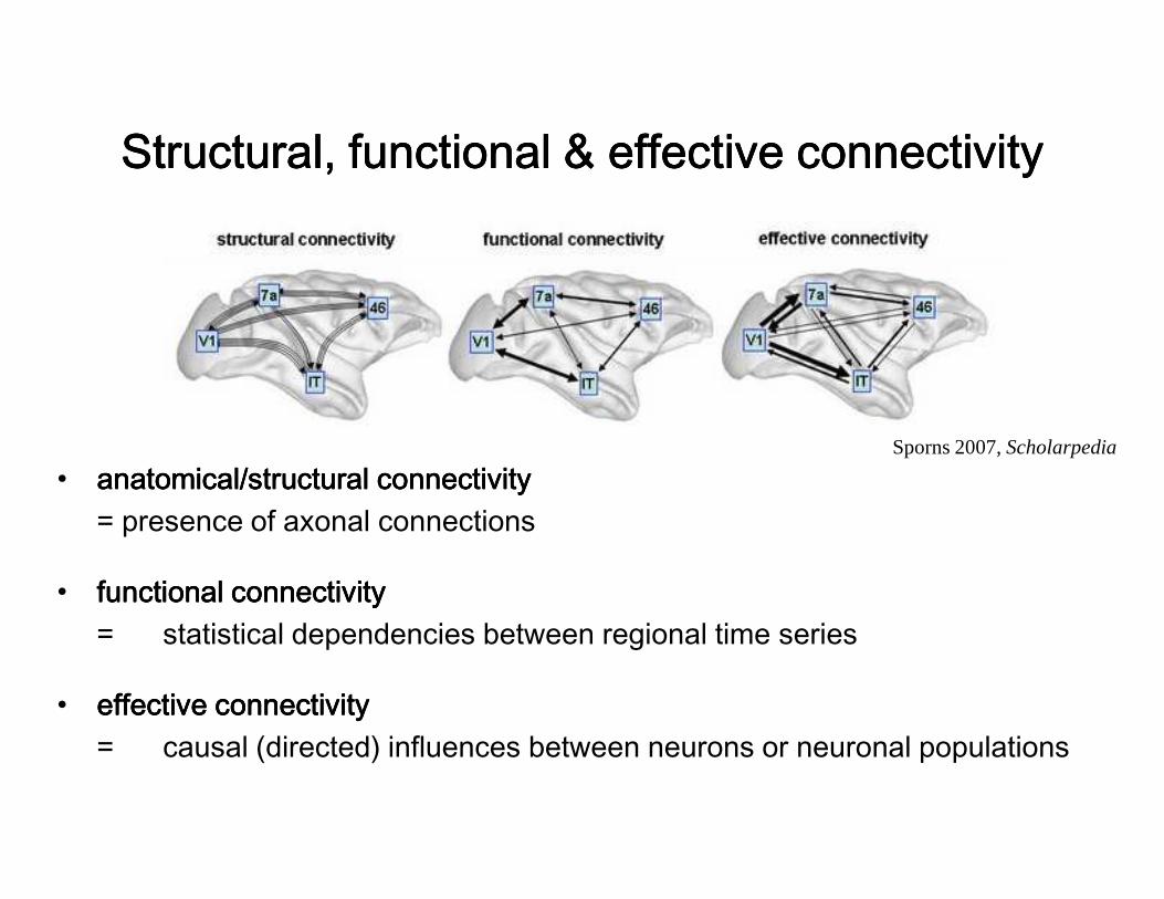
Structural, functional & effective connectivityStructural, functional & effective connectivityStructural, functional & effective connectivityStructural, functional & effective connectivity
• anatomical/structural connectivityanatomical/structural connectivityanatomical/structural connectivityanatomical/structural connectivity= presence of axonal connections
• functional connectivity functional connectivity functional connectivity functional connectivity = statistical dependencies between regional time series
• effective connectivity effective connectivity effective connectivity effective connectivity = causal (directed) influences between neurons or neuronal populations
Structural, functional & effective connectivityStructural, functional & effective connectivityStructural, functional & effective connectivityStructural, functional & effective connectivity
Sporns 2007, Scholarpedia
statistical dependencies between regional time series
causal (directed) influences between neurons or neuronal populations
Sporns 2007, Scholarpedia

Anatomical connectivityAnatomical connectivityAnatomical connectivityAnatomical connectivity
Definition: presence of axonal connections
• neuronal communication via synaptic contacts
• Measured with
– tracing techniques
– diffusion tensor imaging (DTI)
Anatomical connectivityAnatomical connectivityAnatomical connectivityAnatomical connectivity

Knowing Knowing Knowing Knowing anatomical connectivity is not enough...anatomical connectivity is not enough...anatomical connectivity is not enough...anatomical connectivity is not enough...
• Context-dependent recruiting of connections :– Local functions depend on network activity
• Connections show synaptic plasticity– change in the structure and transmission – change in the structure and transmission
properties of a synapse– even at short timescales
�Look at functional and effective connectivity
anatomical connectivity is not enough...anatomical connectivity is not enough...anatomical connectivity is not enough...anatomical connectivity is not enough...
Local functions depend on network activity
Connections show synaptic plasticitychange in the structure and transmission change in the structure and transmission
Look at functional and effective

Definition: statistical dependencies between regional time series
• Seed voxel correlation analysis
• Coherence analysis
Functional connectivityFunctional connectivityFunctional connectivityFunctional connectivity
• Coherence analysis
• Eigen-decomposition (PCA, SVD)
• Independent component analysis (ICA)
• any technique describing statistical dependencies amongst regional time series
Definition: statistical dependencies between regional time series
Seed voxel correlation analysis
Functional connectivityFunctional connectivityFunctional connectivityFunctional connectivity
decomposition (PCA, SVD)
Independent component analysis (ICA)
any technique describing statistical dependencies amongst

SeedSeedSeedSeed----voxel correlation analysesvoxel correlation analysesvoxel correlation analysesvoxel correlation analyses
• hypothesis-driven choice of a seed voxel
• extract reference time seriestime series
• voxel-wise correlation with time series from all other voxels in the brain
voxel correlation analysesvoxel correlation analysesvoxel correlation analysesvoxel correlation analyses
seed voxelseed voxelseed voxelseed voxel

SVCA example: SVCA example: SVCA example: SVCA example: TaskTaskTaskTask----induced changes in functional connectivityinduced changes in functional connectivityinduced changes in functional connectivityinduced changes in functional connectivity
2 bimanual finger2 bimanual finger2 bimanual finger2 bimanual finger----tapping tasks:tapping tasks:tapping tasks:tapping tasks:
During task that required more bimanual coordination, SMA, PPC, M1 and PM showed PPC, M1 and PM showed increased functional connectivity (p<0.001) with left M1
� No difference in SPMs!
Sun et al. 2003, Neuroimage
SVCA example: SVCA example: SVCA example: SVCA example: induced changes in functional connectivityinduced changes in functional connectivityinduced changes in functional connectivityinduced changes in functional connectivity

Does functional connectivity not simply Does functional connectivity not simply Does functional connectivity not simply Does functional connectivity not simply correspond to cocorrespond to cocorrespond to cocorrespond to co----activation in SPMs?activation in SPMs?activation in SPMs?activation in SPMs?
No
Here both areas A1 and A2are correlated identically to
regional regional regional regional response Aresponse Aresponse Aresponse A
are correlated identically to task T, yet they have zero correlation among themselves:
r(A1,T) = r(A2,T) = 0.71butr(A1,A2) = 0 !
Does functional connectivity not simply Does functional connectivity not simply Does functional connectivity not simply Does functional connectivity not simply activation in SPMs?activation in SPMs?activation in SPMs?activation in SPMs?
task Ttask Ttask Ttask T regional response Aregional response Aregional response Aregional response A2222response Aresponse Aresponse Aresponse A1111
Stephan 2004, J. Anat.

Pros & Cons of functional connectivity analysis Pros & Cons of functional connectivity analysis Pros & Cons of functional connectivity analysis Pros & Cons of functional connectivity analysis
• Pros:– useful when we have no experimental control over
the system of interest and no model of what caused the data (e.g. sleep, hallucinations, etc.)
• Cons:• Cons:– interpretation of resulting patterns is difficult / arbitrary – no mechanistic insight– usually suboptimal for situations where we have a
priori knowledge / experimental control
�Effective connectivity
Pros & Cons of functional connectivity analysis Pros & Cons of functional connectivity analysis Pros & Cons of functional connectivity analysis Pros & Cons of functional connectivity analysis
useful when we have no experimental control over the system of interest and no model of what caused the data (e.g. sleep, hallucinations, etc.)
interpretation of resulting patterns is difficult / arbitrary
usually suboptimal for situations where we have a priori knowledge / experimental control

Effective connectivityEffective connectivityEffective connectivityEffective connectivityDefinition: causal causal causal causal (directed) influences between neurons or
neuronal populations
• In vivo and in vitro stimulation and recording••••• Models of causal interactions among neuronal populations
– explain regional effects in terms of
Effective connectivityEffective connectivityEffective connectivityEffective connectivity(directed) influences between neurons or neuronal populations
stimulation and recording
among neuronal populationsin terms of interregional connectivity

Some models for computing effective connectivity Some models for computing effective connectivity Some models for computing effective connectivity Some models for computing effective connectivity from fMRI datafrom fMRI datafrom fMRI datafrom fMRI data
• Structural Equation Modelling (SEM) McIntosh et al. 1991, 1994; Büchel & Friston 1997; Bullmore et al. 2000
• regression models (e.g. psycho-physiological interactions, PPIs)Friston et al. 1997Friston et al. 1997
• Volterra kernels Friston & Büchel 2000
• Time series models (e.g. MAR, Granger causality)Harrison et al. 2003, Goebel et al. 2003
• Dynamic Causal Modelling (DCM)bilinear: Friston et al. 2003; nonlinear: Stephan et al. 2008
Some models for computing effective connectivity Some models for computing effective connectivity Some models for computing effective connectivity Some models for computing effective connectivity from fMRI datafrom fMRI datafrom fMRI datafrom fMRI data
Structural Equation Modelling (SEM) McIntosh et al. 1991, 1994; Büchel & Friston 1997; Bullmore et al. 2000
physiological interactions, PPIs)
Time series models (e.g. MAR, Granger causality)
Dynamic Causal Modelling (DCM)Stephan et al. 2008

PsychoPsychoPsychoPsycho----physiological interaction (PPI)physiological interaction (PPI)physiological interaction (PPI)physiological interaction (PPI)
• bilinear model of how the psychological context the influence of area B on area
B x A → CB x A → C
• A PPI corresponds to differences in regression slopes for different contexts.
physiological interaction (PPI)physiological interaction (PPI)physiological interaction (PPI)physiological interaction (PPI)
bilinear model of how the psychological context A changes on area C :
A PPI corresponds to differences in regression slopes

PsychoPsychoPsychoPsycho----physiological interaction (PPI)physiological interaction (PPI)physiological interaction (PPI)physiological interaction (PPI)Task factor
Task A Task B
Stim
1St
im 2
Stim
ulus
fact
or
A1 B1
A2 B2
We can replace one main effect in the GLM by the time series of an area that shows this main effect.
Stim
2
Stim
ulus
fact
or
Friston et al. 1997, NeuroImage
physiological interaction (PPI)physiological interaction (PPI)physiological interaction (PPI)physiological interaction (PPI)
e
βSSTT
βSS
TT y
BA
BA
+−−+
−+−=
321
221
1
)( )(
)(
)( β
GLM of a 2x2 factorial design:
main effectof task
main effectof stim. type
interaction
We can replace one main effect in
e
βVTT
βV
TT y
BA
BA
+−+
+−=
3
2
1
1 )(
1
)( β
e+
main effectof task
V1 time series ≈ main effectof stim. typepsycho-physiologicalinteraction

V1V1 V5V5
AttentionAttentionAttentionAttention
Example PPI: Attentional modulation of V1Example PPI: Attentional modulation of V1Example PPI: Attentional modulation of V1Example PPI: Attentional modulation of V1
Friston et al. 1997, NeuroImageBüchel & Friston 1997, Cereb. Cortex
V1 x Att.V1 x Att.
====
V5V5
SPM{Z}
V5 a
ctiv
ity
Example PPI: Attentional modulation of V1Example PPI: Attentional modulation of V1Example PPI: Attentional modulation of V1Example PPI: Attentional modulation of V1→V5→V5→V5→V5
attentionattentionattentionattention
no attentionno attentionno attentionno attention
V1 activity
V5 a
ctiv
ity
time
Pros & Cons of PPIsPros & Cons of PPIsPros & Cons of PPIsPros & Cons of PPIs• Pros:
– given a single source region, we can test for its contextconnectivity across the entire brain
– easy to implement
• Cons:– only allows to model contributions from a single area – only allows to model contributions from a single area – operates at the level of BOLD time series– ignores time-series properties of the data
Dynamic Causal Models
Pros & Cons of PPIsPros & Cons of PPIsPros & Cons of PPIsPros & Cons of PPIs
given a single source region, we can test for its context-dependent connectivity across the entire brain
only allows to model contributions from a single area only allows to model contributions from a single area operates at the level of BOLD time series
series properties of the data
Dynamic Causal Models

OverviewOverviewOverviewOverview
• Brain connectivity: types & definitions
• Functional connectivity
• Psycho-physiological interactions (PPI)
• Dynamic causal models (DCMs)• Dynamic causal models (DCMs)– Basic idea– Neural level– Hemodynamic level– Parameter estimation, priors & inference
• Applications of DCM to fMRI data
OverviewOverviewOverviewOverview
Brain connectivity: types & definitions
physiological interactions (PPI)
Dynamic causal models (DCMs)Dynamic causal models (DCMs)
Parameter estimation, priors & inference
Applications of DCM to fMRI data
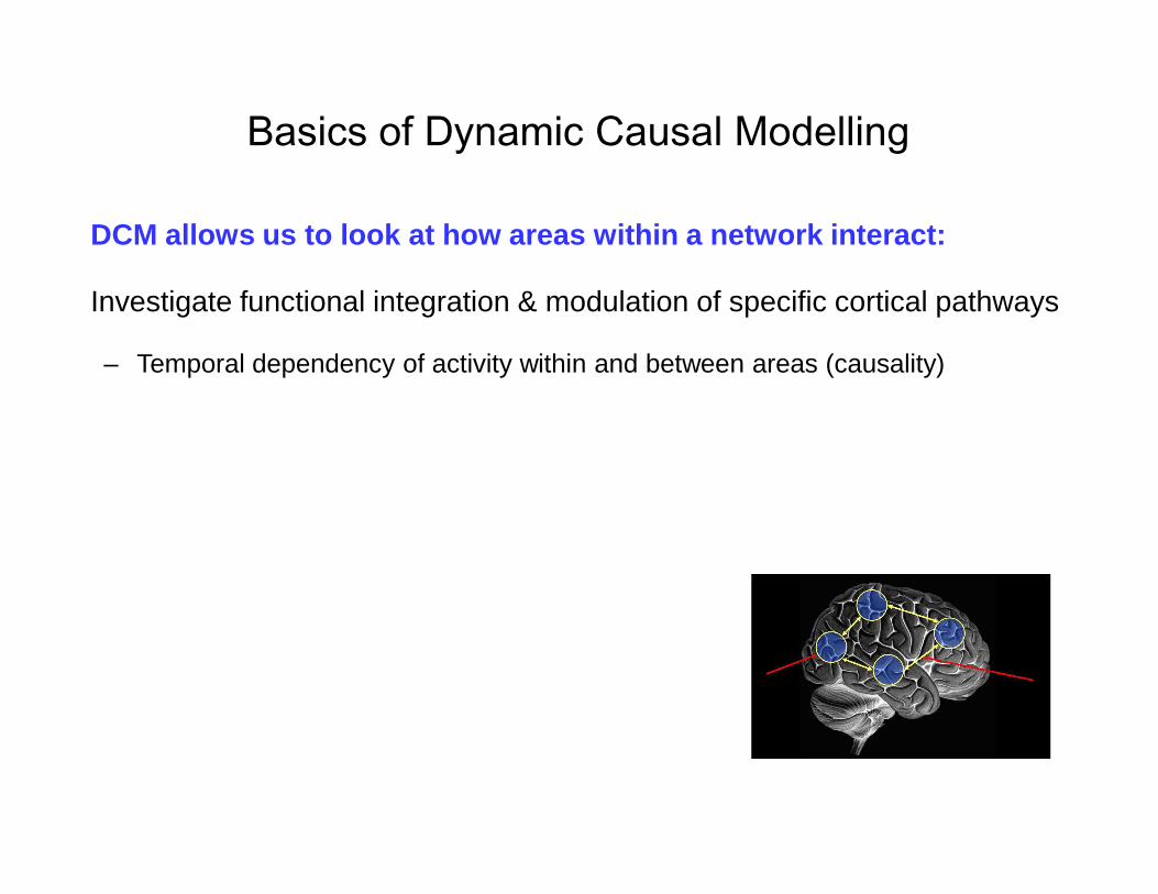
Basics of Dynamic Causal Modelling
DCM allows us to look at how areas within a network interact:
Investigate functional integration & modulation of specific cortical pathways
– Temporal dependency of activity within and between areas (causality)
Basics of Dynamic Causal Modelling
DCM allows us to look at how areas within a network interact:
Investigate functional integration & modulation of specific cortical pathways
Temporal dependency of activity within and between areas (causality)

Temporal dependence and causal relations
Seed voxel approach, PPI etc.
timeseries (neuronal activity)
Temporal dependence and causal relations
Dynamic Causal Models
timeseries (neuronal activity)

Basics of Dynamic Causal Modelling
DCM allows us to look at how areas within a network interact:
Investigate functional integration & modulation of specific cortical pathways
– Temporal dependency of activity within and between areas (causality)
– Separate neuronal activity from observed BOLD responses
Basics of Dynamic Causal Modelling
DCM allows us to look at how areas within a network interact:
Investigate functional integration & modulation of specific cortical pathways
Temporal dependency of activity within and between areas (causality)
Separate neuronal activity from observed BOLD responses

• Cognitive system is modelled at its underlying neuronal level (not directly accessible for
• The modelled neuronal dynamics (x) are transformed into area-specific BOLD signals (a hemodynamic model (λλλλ).
Basics of DCM: Basics of DCM: Basics of DCM: Basics of DCM: Neuronal and BOLD levelNeuronal and BOLD levelNeuronal and BOLD levelNeuronal and BOLD level
a hemodynamic model (λλλλ).
The aim of DCM is to estimate parameters at the neuronal level such that the modelled and measured BOLD signals are maximally* similar.
Cognitive system is modelled at its underlying (not directly accessible for fMRI).
) are specific BOLD signals (y) by
x
Basics of DCM: Basics of DCM: Basics of DCM: Basics of DCM: Neuronal and BOLD levelNeuronal and BOLD levelNeuronal and BOLD levelNeuronal and BOLD level
λ
y
parameters such that the modelled

DCM: Linear ModelDCM: Linear ModelDCM: Linear ModelDCM: Linear Model
3232221212
1112121111
xaxaxax
ucxaxax
+=++=++=
&
&
X1X1X1X1 X2X2X2X2 X3X3X3X3u1u1u1u1
3332323 xaxax +=&
=
3
2
1
3332
232221
1211
3
2
1
0
0
x
x
x
aa
aaa
aa
x
x
x
&
&
&
effectiveeffectiveeffectiveeffectiveconnectivityconnectivityconnectivityconnectivity
state state state state changeschangeschangeschanges
systemsystemsystemsystemstatestatestatestate
DCM: Linear ModelDCM: Linear ModelDCM: Linear ModelDCM: Linear Model
{ }CA
CuAxx
,=+=
θ&
+
3
2
111
000
000
00
u
u
uc
externalexternalexternalexternalinputsinputsinputsinputs
inputinputinputinputparametersparametersparametersparameters
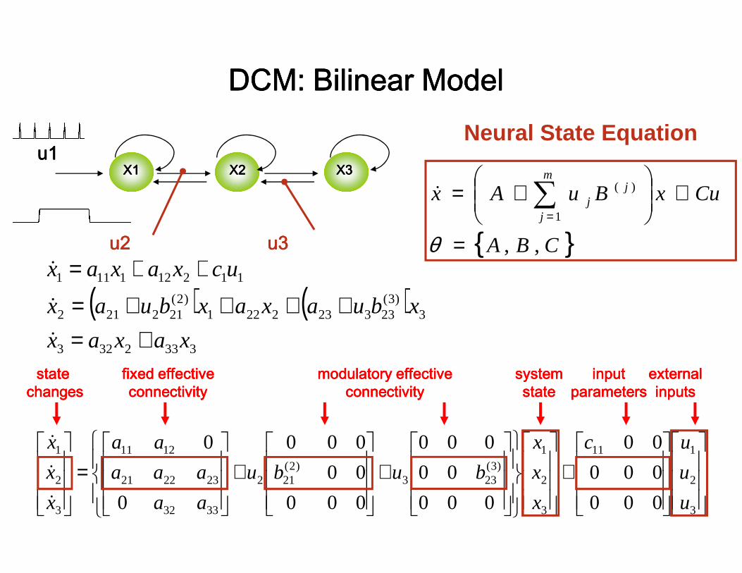
DCM: Bilinear ModelDCM: Bilinear ModelDCM: Bilinear ModelDCM: Bilinear Model
( ) (112121111 ucxaxax ++=&
X1X1X1X1 X2X2X2X2 X3X3X3X3u1u1u1u1
u2u2u2u2 u3u3u3u3
+
=
)2(
212
3332
232221
1211
3
2
1
000
00
000
0
0
bu
aa
aaa
aa
x
x
x
&
&
&
( ) (3332323
3232221)2(
212212
xaxax
buaxaxbuax
+=++++=
&
&
fixed effectivefixed effectivefixed effectivefixed effectiveconnectivityconnectivityconnectivityconnectivity
state state state state changeschangeschangeschanges
modulatory effectivemodulatory effectivemodulatory effectivemodulatory effectiveconnectivityconnectivityconnectivityconnectivity
DCM: Bilinear ModelDCM: Bilinear ModelDCM: Bilinear ModelDCM: Bilinear Model
{ }CBA
CuxBuAxm
j
jj
,,
1
)(
=
+
+= ∑
=
θ
&
Neural State Equation
)
+
+
3
2
111
3
2
1)3(
233
000
000
00
000
00
000
u
u
uc
x
x
x
bu
) 3)3(
23 xb
systemsystemsystemsystemstatestatestatestate
inputinputinputinputparametersparametersparametersparameters
externalexternalexternalexternalinputsinputsinputsinputs
modulatory effectivemodulatory effectivemodulatory effectivemodulatory effectiveconnectivityconnectivityconnectivityconnectivity

• Cognitive system is modelled at its underlying neuronal level (not directly accessible for
• The modelled neuronal dynamics (x) are transformed into area-specific BOLD signals (a hemodynamic model (λ).
Basics of DCM: Basics of DCM: Basics of DCM: Basics of DCM: Neuronal and BOLD levelNeuronal and BOLD levelNeuronal and BOLD levelNeuronal and BOLD level
a hemodynamic model (λ).
Cognitive system is modelled at its underlying (not directly accessible for fMRI).
) are specific BOLD signals (y) by
x
Basics of DCM: Basics of DCM: Basics of DCM: Basics of DCM: Neuronal and BOLD levelNeuronal and BOLD levelNeuronal and BOLD levelNeuronal and BOLD level
λ
y

important for model fitting, but of no interest for statistical inference
The hThe hThe hThe hemodynamic modelemodynamic modelemodynamic modelemodynamic model• 6 hemodynamic
parameters:
of no interest for statistical inference
• Computed separately for each area → region-specific HRFs!
Friston et al. 2000, NeuroImageStephan et al. 2007, NeuroImage
emodynamic modelemodynamic modelemodynamic modelemodynamic model
)(
activity
tx
sf
)1(
−−−= fγsxs
signalryvasodilato
κ&s
stimulus functionsstimulus functionsstimulus functionsstimulus functionsut
neural state equationneural state equationneural state equationneural state equation
hemodynamic state hemodynamic state hemodynamic state hemodynamic state
( ) ,)(
signal BOLD
qvty λ=
sf
tionflow induc
=& (rCBF)
v
v
q q/vvEf,EEfqτ /α
dHbchanges in
100)( −=&/αvfvτ
volumechanges in
1−=&q
f
hemodynamic state hemodynamic state hemodynamic state hemodynamic state equationsequationsequationsequations
Estimated BOLD Estimated BOLD Estimated BOLD Estimated BOLD responseresponseresponseresponse

Measured vs Modelled BOLD signalMeasured vs Modelled BOLD signalMeasured vs Modelled BOLD signalMeasured vs Modelled BOLD signalRecapRecapRecapRecapThe aim of DCM is to estimate- neural parameters {A, B, C}- hemodynamic parameters such that the modelled modelled modelled modelled and measured measured measured measured BOLD signals are maximally similar
u1u1u1u1u1u1u1u1
Measured vs Modelled BOLD signalMeasured vs Modelled BOLD signalMeasured vs Modelled BOLD signalMeasured vs Modelled BOLD signal
BOLD signals are maximally similar.
X1X1X1X1 X2X2X2X2 X3X3X3X3
u2u2u2u2 u3u3u3u3
yyy
activityx1(t)
activityx2(t) activity
x3(t)
neuronalstates
modulatoryinput u2(t)
endogenous connectivity
direct inputs
modulation ofconnectivity
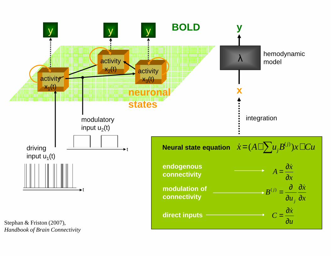
Neural state equation
t
drivinginput u1(t)
input u2(t)
t
Stephan & Friston (2007),Handbook of Brain Connectivity
hemodynamicmodelλ
x
y
integration
BOLD
neuronal
endogenous connectivity
direct inputs
modulation ofconnectivity
Neural state equation CuxBuAx jj ++= ∑ )( )(
&
u
xC
x
x
uB
x
xA
j
j
∂∂=
∂∂
∂∂=
∂∂=
&
&
&
)(

OverviewOverviewOverviewOverview
• Brain connectivity: types & definitions
• Functional connectivity
• Psycho-physiological interactions (PPI)
• Dynamic causal models (DCMs)• Dynamic causal models (DCMs)– Basic idea– Neural level– Hemodynamic level– Parameter estimation, priors & inference
• Applications of DCM to fMRI data
OverviewOverviewOverviewOverview
Brain connectivity: types & definitions
physiological interactions (PPI)
Dynamic causal models (DCMs)Dynamic causal models (DCMs)
Parameter estimation, priors & inference
Applications of DCM to fMRI data

DCM parameters = rate constantsDCM parameters = rate constantsDCM parameters = rate constantsDCM parameters = rate constants
dxax
dt= 0( ) exp( )x t x at=
The coupling parameter a determines
Integration of a first-order linear differential equation gives anexponential function:
The coupling parameter a determines the half life of x(t), and thus describes the speed of the exponential change
If AIf AIf AIf A����B is 0.10 sB is 0.10 sB is 0.10 sB is 0.10 s----1111 this means that, this means that, this means that, this means that, activity in B corresponds to 10% of the activity in Aactivity in B corresponds to 10% of the activity in Aactivity in B corresponds to 10% of the activity in Aactivity in B corresponds to 10% of the activity in A
DCM parameters = rate constantsDCM parameters = rate constantsDCM parameters = rate constantsDCM parameters = rate constants
( ) exp( )x t x at
order linear differential equation gives an
0.5x00.5x
a/2ln=τ
this means that, this means that, this means that, this means that, per unit time, the increase in per unit time, the increase in per unit time, the increase in per unit time, the increase in activity in B corresponds to 10% of the activity in Aactivity in B corresponds to 10% of the activity in Aactivity in B corresponds to 10% of the activity in Aactivity in B corresponds to 10% of the activity in A
stimuliu1
contextu2
x1
-
-+
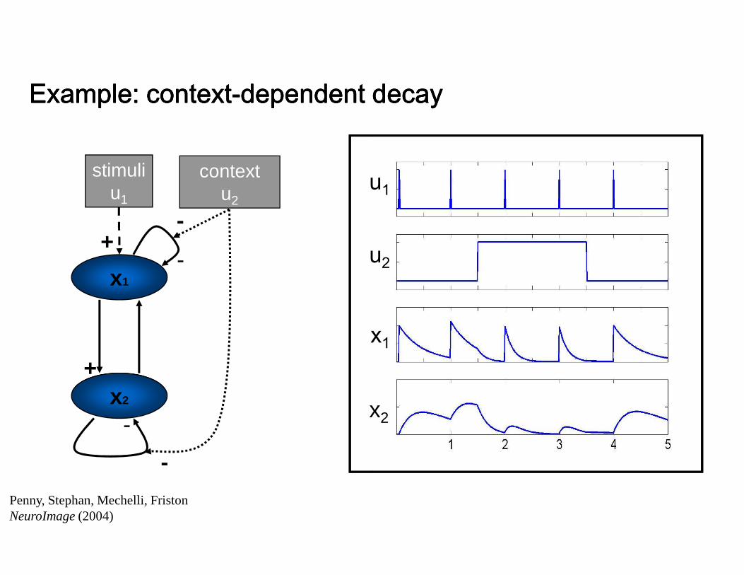
Example: contextExample: contextExample: contextExample: context----dependent decaydependent decaydependent decaydependent decay
u1
Z1
u2
u
u
-
x2
x1
+
+
-
Z1
Z2
x
x
Penny, Stephan, Mechelli, Friston NeuroImage (2004)
dependent decaydependent decaydependent decaydependent decay
u1
Z1
u2
u1
u2Z1
Z2
x2
x1

Conceptual overviewConceptual overviewConceptual overviewConceptual overview
Neuronal states
cccc2222
cccc1111
Driving inputDriving inputDriving inputDriving input(e.g. sensory stim
Modulatory inputModulatory inputModulatory inputModulatory input(e.g. context/learning/drugs)
bbbb12121212
yy
activityx1(t) aaaa12121212 activity
x2(t)
BOLD Response
Conceptual overviewConceptual overviewConceptual overviewConceptual overview
sensory stim) Parameters are optimised
so that the predicted
matches the measured
BOLD responseBOLD response
�How confident are we
about these parameters?

Bayesian statisticsBayesian statisticsBayesian statisticsBayesian statistics
posterior posterior posterior posterior ∝∝∝∝ likelihood likelihood likelihood likelihood ∙ ∙ ∙ ∙ priorpriorpriorprior
Express our prior knowledgeprior knowledgeprior knowledgeprior knowledge or “belief” about parameters of the model
new datanew datanew datanew data prior knowledgeprior knowledgeprior knowledgeprior knowledge
posterior posterior posterior posterior ∝∝∝∝ likelihood likelihood likelihood likelihood ∙ ∙ ∙ ∙ priorpriorpriorprior
Bayesian statisticsBayesian statisticsBayesian statisticsBayesian statisticsor “belief” about parameters of the model
Parameters governing• Hemodynamics in a single region• Neuronal interactions
Constraints (priors) onConstraints (priors) on• Hemodynamic parameters
- empirical
• Self connections-principled
• Other connections- shrinkage

Inference about DCM parametersInference about DCM parametersInference about DCM parametersInference about DCM parameters
Bayesian single subject analysis
• The model parameters are distributions that have a mean ηθ|yand covariance Cθ|y.
– Use of the cumulative normal distribution to test the probability distribution to test the probability that a certain parameter is above a chosen threshold γ:
γ ηθ|y
Inference about DCM parametersInference about DCM parametersInference about DCM parametersInference about DCM parameters
Classical frequentist test across Ss
• Test summary statistic: mean ηθ|y
– One-sample t-test: Parameter > 0?
– Paired t-test:parameter 1 > parameter 2?
– Paired t-test:parameter 1 > parameter 2?
– rmANOVA: e.g. in case of multiple sessions per subject
Bayesian model averaging

Inference about model spaceInference about model spaceInference about model spaceInference about model space
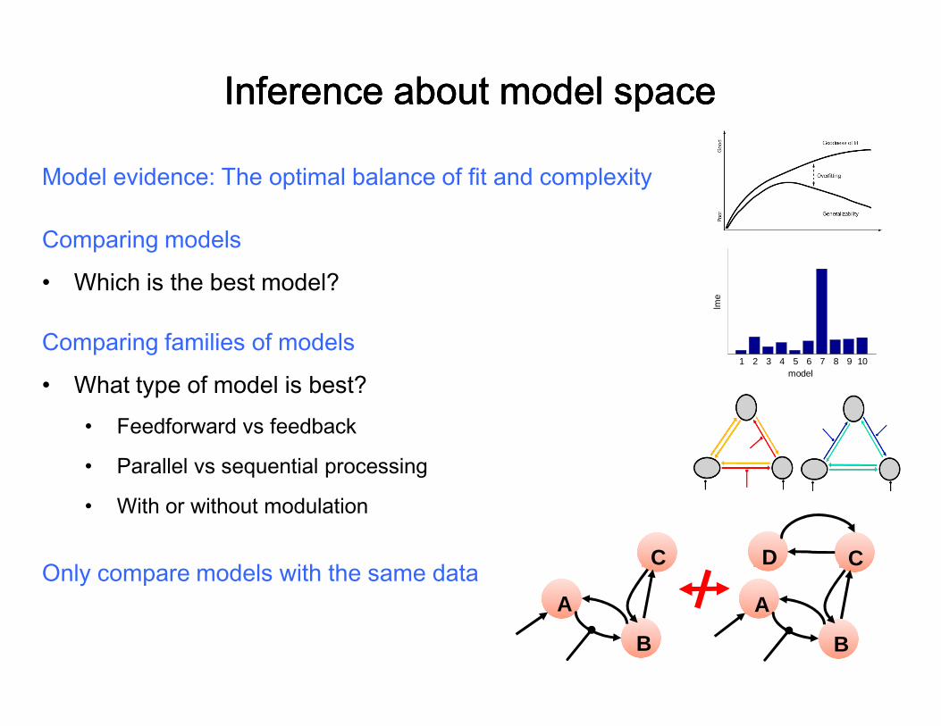
Model evidence: The optimal balance of fit and complexity
Inference about model spaceInference about model spaceInference about model spaceInference about model space
Model evidence: The optimal balance of fit and complexity
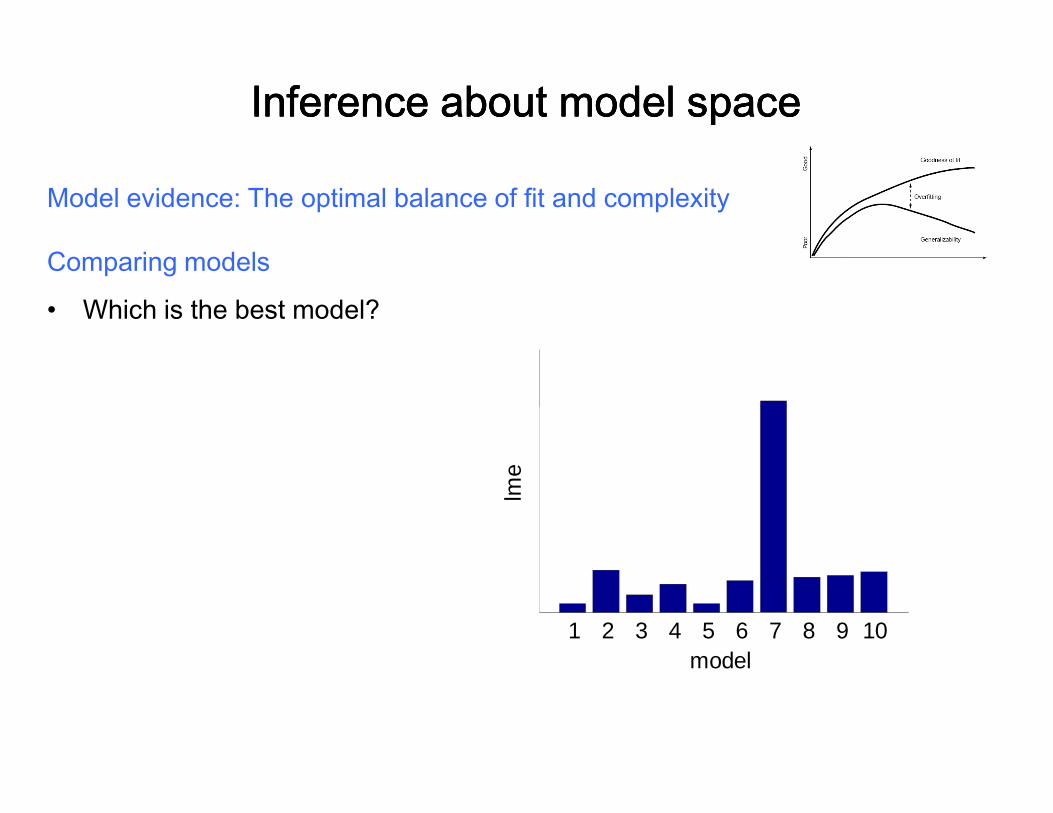
Inference about model spaceInference about model spaceInference about model spaceInference about model space
Model evidence: The optimal balance of fit and complexity
Comparing models
• Which is the best model?
lme
Inference about model spaceInference about model spaceInference about model spaceInference about model space
Model evidence: The optimal balance of fit and complexity
1 2 3 4 5 6 7 8 9 10model
Inference about model spaceInference about model spaceInference about model spaceInference about model space
Model evidence: The optimal balance of fit and complexity
Comparing models
• Which is the best model?
Comparing families of models
• What type of model is best?• Feedforward vs feedback
• Parallel vs sequential processing
• With or without modulation
Inference about model spaceInference about model spaceInference about model spaceInference about model space
Model evidence: The optimal balance of fit and complexity
1 2 3 4 5 6 7 8 9 10
lme
1 2 3 4 5 6 7 8 9 10model
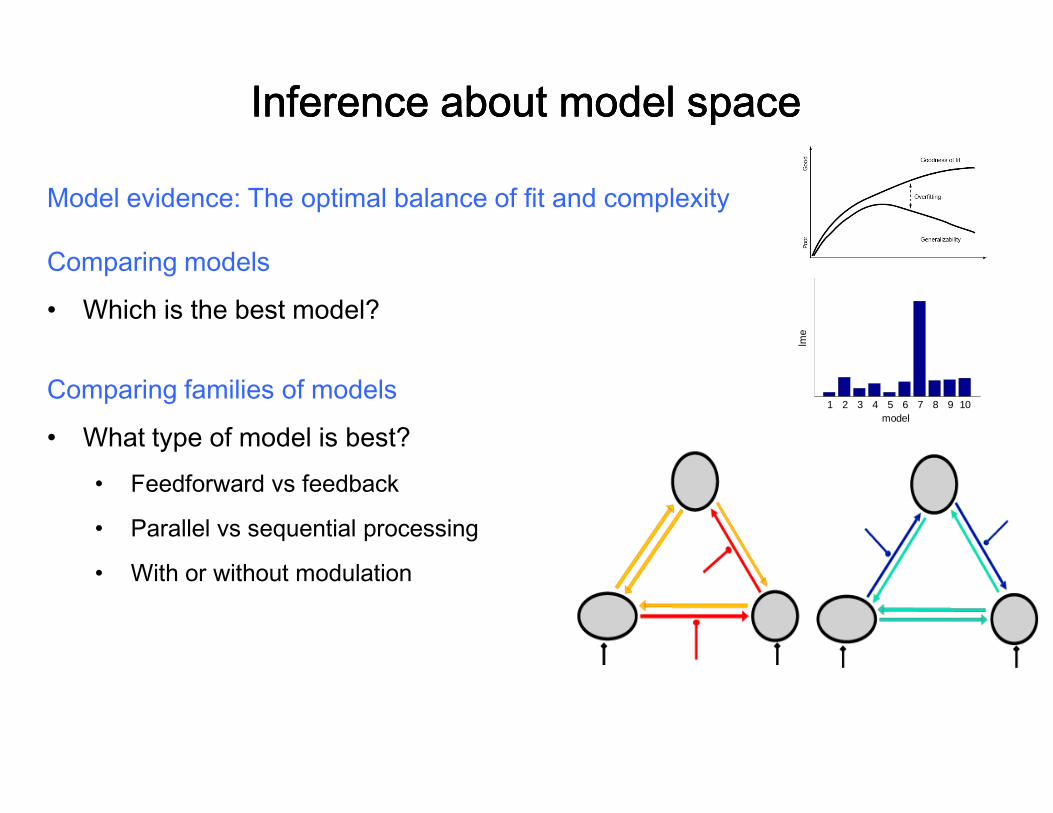
Inference about model spaceInference about model spaceInference about model spaceInference about model space
Model evidence: The optimal balance of fit and complexity
Comparing models
• Which is the best model?
Comparing families of models
• What type of model is best?• Feedforward vs feedback
• Parallel vs sequential processing
• With or without modulation
Only compare models with the same data
Inference about model spaceInference about model spaceInference about model spaceInference about model space
Model evidence: The optimal balance of fit and complexity
1 2 3 4 5 6 7 8 9 10
lme
Only compare models with the same data
1 2 3 4 5 6 7 8 9 10model
A
D
B
C
A
B
C

OverviewOverviewOverviewOverview
• Brain connectivity: types & definitions
• Functional connectivity
• Psycho-physiological interactions (PPI)
• Dynamic causal models (DCMs)• Dynamic causal models (DCMs)
• Applications of DCM to fMRI data– Design of experiments and models– Generating data
OverviewOverviewOverviewOverview
Brain connectivity: types & definitions
physiological interactions (PPI)
Dynamic causal models (DCMs)Dynamic causal models (DCMs)
Applications of DCM to fMRI dataDesign of experiments and models

Planning a DCMPlanning a DCMPlanning a DCMPlanning a DCM----
• Suitable experimental design:– any design that is suitable for a GLM – preferably multi-factorial (e.g. 2 x 2)
• e.g. one factor that varies the driving• and one factor that varies the contextual
• Hypothesis and model:– Define specific a priori hypothesis– Which parameters are relevant to test this hypothesis?– If you want to verify that intended model is suitable to test this hypothesis,
then use simulations– Define criteria for inference– What are the alternative models to test?
----compatible studycompatible studycompatible studycompatible study
any design that is suitable for a GLM factorial (e.g. 2 x 2)
driving (sensory) inputcontextual input
Which parameters are relevant to test this hypothesis?If you want to verify that intended model is suitable to test this hypothesis,
What are the alternative models to test?

Multifactorial design: Multifactorial design: Multifactorial design: Multifactorial design: explaining interactions with DCMexplaining interactions with DCMexplaining interactions with DCMexplaining interactions with DCM
Task factorTask A Task B
Stim
1St
im 2
Stim
ulus
fact
or
A1 B1
Stim
2St
imul
us fa
ctor
A2 B2
Let’s assume that an SPM analysis shows a main effect of stimulus in X1 and a stimulus × task interaction in X2.
How do we model this using DCM?
Multifactorial design: Multifactorial design: Multifactorial design: Multifactorial design: explaining interactions with DCMexplaining interactions with DCMexplaining interactions with DCMexplaining interactions with DCM
XXXX1111 XXXX2222
Stim2/Stim2/Stim2/Stim2/Task ATask ATask ATask A
Stim1/Stim1/Stim1/Stim1/Task ATask ATask ATask A
GLMGLMGLMGLM
Stim 1/Stim 1/Stim 1/Stim 1/Task BTask BTask BTask B
Stim 2/Stim 2/Stim 2/Stim 2/Task BTask BTask BTask B
XXXX1111 XXXX2222
Stim2Stim2Stim2Stim2
Stim1Stim1Stim1Stim1
Task ATask ATask ATask A Task BTask BTask BTask B
DCMDCMDCMDCM

X1X1X1X1 X2X2X2X2
Stim1Stim1Stim1Stim1
Simulated dataSimulated dataSimulated dataSimulated data
++++++++++++
++++
++++++++++++X1X1X1X1 X2X2X2X2
Stim2Stim2Stim2Stim2Task ATask ATask ATask A Task BTask BTask BTask B
++++++++++++++++++++
++++++++++++Stim 1Stim 1Stim 1Stim 1Task ATask ATask ATask A
Stim 2Stim 2Stim 2Stim 2Task ATask ATask ATask A
Stim 1Stim 1Stim 1Stim 1Task BTask BTask BTask B
Stim 2Stim 2Stim 2Stim 2Task BTask BTask BTask B
X1X1X1X1
Task ATask ATask ATask A Task ATask ATask ATask A Task BTask BTask BTask B Task BTask BTask BTask B
X2X2X2X2

Stim 1Stim 1Stim 1Stim 1Task ATask ATask ATask A
Stim 2Stim 2Stim 2Stim 2Task ATask ATask ATask A
Stim 1Stim 1Stim 1Stim 1Task BTask BTask BTask B
Stim 2Stim 2Stim 2Stim 2Task BTask BTask BTask B
XXXX1111
Task ATask ATask ATask A Task ATask ATask ATask A Task BTask BTask BTask B Task BTask BTask BTask B
plus added noise (SNR=1)plus added noise (SNR=1)plus added noise (SNR=1)plus added noise (SNR=1)
XXXX2222
plus added noise (SNR=1)plus added noise (SNR=1)plus added noise (SNR=1)plus added noise (SNR=1)

DCM roadmapDCM roadmapDCM roadmapDCM roadmap
Neuronal dynamics
State space Model
fMRI data
Bayesian Model inversion
Model
Priors
DCM roadmapDCM roadmapDCM roadmapDCM roadmap
Haemodynamics
State space Model
Posterior densities of parameters
Model comparison
Bayesian Model inversion
Model
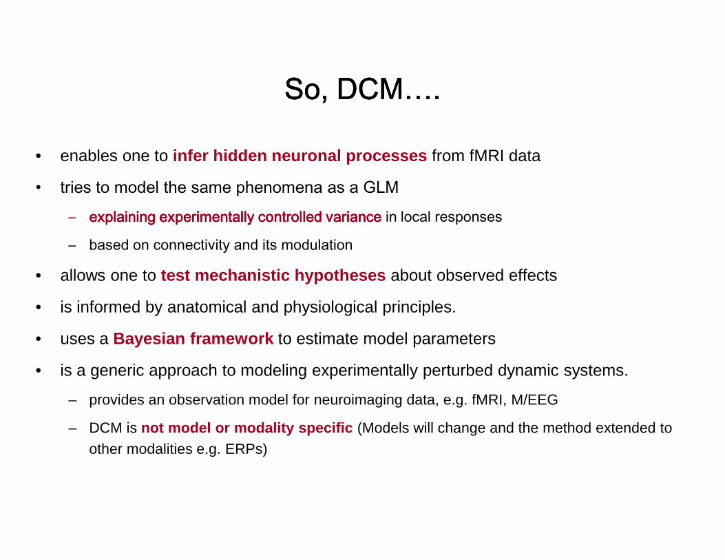
So, DCM….So, DCM….So, DCM….So, DCM….
• enables one to infer hidden neuronal processes
• tries to model the same phenomena as a GLM– explaining experimentally controlled varianceexplaining experimentally controlled varianceexplaining experimentally controlled varianceexplaining experimentally controlled variance
– based on connectivity and its modulation
• allows one to test mechanistic hypotheses • allows one to test mechanistic hypotheses
• is informed by anatomical and physiological principles.
• uses a Bayesian framework to estimate model parameters
• is a generic approach to modeling experimentally perturbed dynamic systems.
– provides an observation model for neuroimaging data, e.g. fMRI, M/EEG
– DCM is not model or modality specific (Models will change and the method extended to other modalities e.g. ERPs)
So, DCM….So, DCM….So, DCM….So, DCM….
infer hidden neuronal processes from fMRI data
tries to model the same phenomena as a GLMexplaining experimentally controlled varianceexplaining experimentally controlled varianceexplaining experimentally controlled varianceexplaining experimentally controlled variance in local responses
test mechanistic hypotheses about observed effectstest mechanistic hypotheses about observed effects
is informed by anatomical and physiological principles.
to estimate model parameters
is a generic approach to modeling experimentally perturbed dynamic systems.
provides an observation model for neuroimaging data, e.g. fMRI, M/EEG
(Models will change and the method extended to

Some useful referencesSome useful referencesSome useful referencesSome useful references• The first DCM paper: Dynamic Causal Modelling (2003). Friston et al.
NeuroImage 19:1273-1302.
• Physiological validation of DCM for fMRI:functional MRI: an electrophysiological validation (2008). David et al. Biol. 6 2683–2697
• Hemodynamic model: Comparing hemodynamic models with DCM (2007). Stephan et al. NeuroImage 38:387-401Stephan et al. NeuroImage 38:387-401
• Nonlinear DCMs: Nonlinear Dynamic Causal Models for FMRI (2008). Stephan et al. NeuroImage 42:649-662
• Two-state model: Dynamic causal modelling for fMRI: A two(2008). Marreiros et al. NeuroImage 39:269
• Group Bayesian model comparison:studies (2009). Stephan et al. NeuroImage
• 10 Simple Rules for DCM (2010). Stephan et al
Some useful referencesSome useful referencesSome useful referencesSome useful referencesDynamic Causal Modelling (2003). Friston et al.
Physiological validation of DCM for fMRI: Identifying neural drivers with functional MRI: an electrophysiological validation (2008). David et al. PLoS
Comparing hemodynamic models with DCM (2007). 401401
Nonlinear Dynamic Causal Models for FMRI (2008). Stephan
Dynamic causal modelling for fMRI: A two-state model 39:269-278
Bayesian model selection for group NeuroImage 46:1004-10174
(2010). Stephan et al. NeuroImage 52.

Thank youThank youThank youThank youThank youThank youThank youThank you

Time to do a DCM!Time to do a DCM!Time to do a DCM!Time to do a DCM!Time to do a DCM!Time to do a DCM!Time to do a DCM!Time to do a DCM!

Dynamic Causal ModellingPRACTICAL
Andre Marreiros
Functional Imaging Laboratory (FIL)Wellcome Trust Centre for NeuroimagingWellcome Trust Centre for NeuroimagingUniversity College London
Hanneke den Ouden
Donders Centre for Cognitive NeuroimagingRadboud University Nijmegen
Dynamic Causal ModellingPRACTICAL
SPM Course, London13-15 May 2010
Donders Centre for Cognitive Neuroimaging

DCM – Attention to MotionParadigm Stimuli 250 radially moving dots at 4.7 degrees/s
Pre-Scanning5 x 30s trials with 5 speed changes (reducing to 1%)Task - detect change in radial velocity
Scanning (no speed changes)F A F N F A F N S ….
Attention to Motion in the visual system
Parameters - blocks of 10 scans - 360 scans total- TR = 3.22 seconds
F A F N F A F N S ….F - fixation S - observe static dotsN - observe moving dotsA - attend moving dots
Attention to Motion250 radially moving dots at 4.7 degrees/s
5 x 30s trials with 5 speed changes (reducing to 1%)detect change in radial velocity
(no speed changes)F A F N F A F N S ….
Attention to Motion in the visual system
blocks of 10 scans 360 scans totalTR = 3.22 seconds
F A F N F A F N S ….fixation observe static dots + photicobserve moving dots + motionattend moving dots + attention
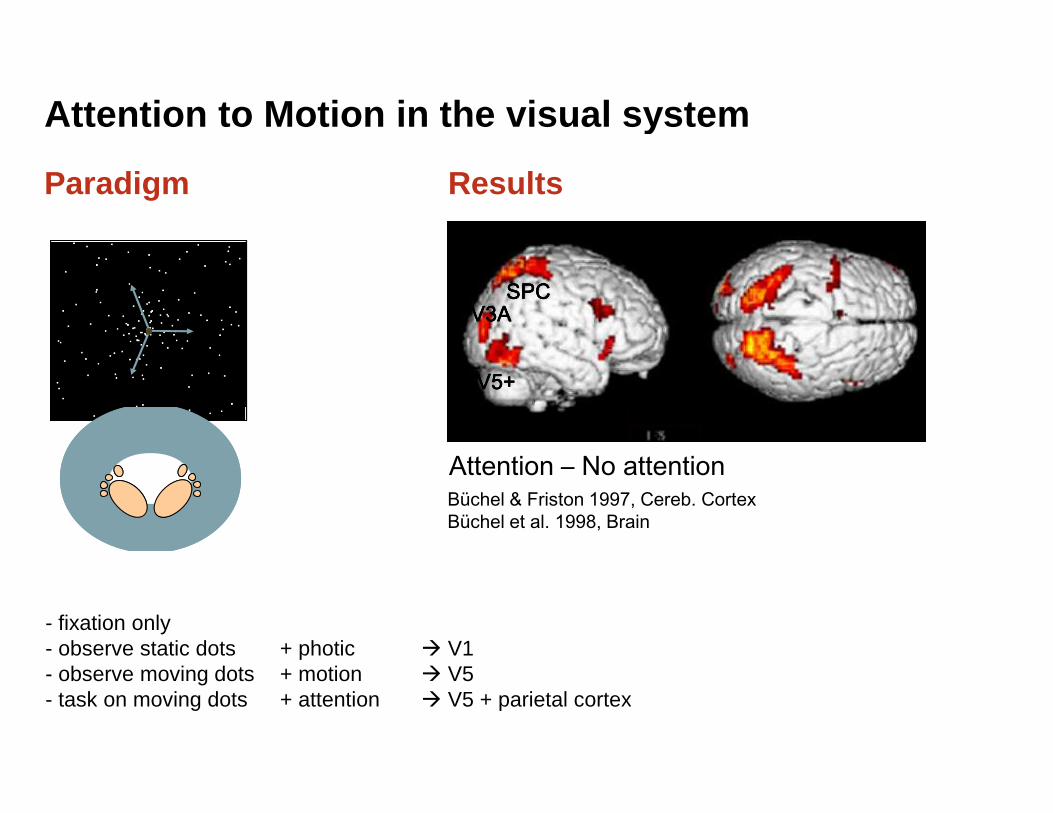
Results
V5+V5+V5+V5+
SPCSPCSPCSPCV3AV3AV3AV3A
Attention to Motion in the visual system
Paradigm
Büchel & Friston 1997, Cereb. CortexBüchel et al.
Attention
- fixation only- observe static dots + photic � V1- observe moving dots + motion � V5- task on moving dots + attention � V5 + parietal cortex
Results
SPCSPCSPCSPC
Attention to Motion in the visual system
chel & Friston 1997, Cereb. Cortexchel et al. 1998, Brain
Attention – No attention
V5 + parietal cortex

SPCSPCSPCSPCPhotic Photic
Model 1Model 1Model 1Model 1attentional modulationof V1→V5: forward
Model 2Model 2Model 2Model 2attentional modulationof SPC→V5: backward
DCM: comparison of 2 models
V1V1V1V1
V5V5V5V5
MotionAttention
Photic
Bayesian model selection: Which model is optimal?Bayesian model selection: Which model is optimal?Bayesian model selection: Which model is optimal?Bayesian model selection: Which model is optimal?
SPCSPCSPCSPCPhoticAttention
Model 2Model 2Model 2Model 2attentional modulationof SPC→V5: backward
DCM: comparison of 2 models
V1V1V1V1
V5V5V5V5
SPCSPCSPCSPC
Motion
Photic
Bayesian model selection: Which model is optimal?Bayesian model selection: Which model is optimal?Bayesian model selection: Which model is optimal?Bayesian model selection: Which model is optimal?
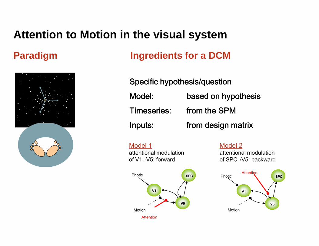
Ingredients for a DCM
Specific hypothesis/questionSpecific hypothesis/questionSpecific hypothesis/questionSpecific hypothesis/question
Model: Model: Model: Model:
Timeseries: Timeseries: Timeseries: Timeseries:
Inputs: Inputs: Inputs: Inputs:
Attention to Motion in the visual system
Paradigm
Inputs: Inputs: Inputs: Inputs:
V1V1V1V1
Motion
Photic
Attention
Model 1attentional modulationof V1→V5: forward
Ingredients for a DCM
Specific hypothesis/questionSpecific hypothesis/questionSpecific hypothesis/questionSpecific hypothesis/question
based on hypothesisbased on hypothesisbased on hypothesisbased on hypothesis
Timeseries: Timeseries: Timeseries: Timeseries: from the SPMfrom the SPMfrom the SPMfrom the SPM
from design matrixfrom design matrixfrom design matrixfrom design matrix
Attention to Motion in the visual system
from design matrixfrom design matrixfrom design matrixfrom design matrix
V5V5V5V5
SPCSPCSPCSPC
V1V1V1V1
V5V5V5V5
SPCSPCSPCSPC
Motion
PhoticAttention
attentional modulationof V1→V5: forward
Model 2attentional modulationof SPC→V5: backward

DCM – GUI basic steps
1 – Extract the time series (from all regions of interest)
2 – Specify the model
Attention to Motion in the visual system
3 – Estimate the model
4 – Review the estimated model
5 – Repeat steps 2 and 3 for all models in model space
6 – Compare models
Extract the time series (from all regions of interest)
Attention to Motion in the visual system
Repeat steps 2 and 3 for all models in model space


![Bayesian Causal Inference - uni-muenchen.de...from causal inference have been attracting much interest recently. [HHH18] propose that causal [HHH18] propose that causal inference stands](https://img.dokumen.tips/doc/110x75/5ec457b21b32702dbe2c9d4c/bayesian-causal-inference-uni-from-causal-inference-have-been-attracting.jpg)


![Comparing Dynamic Causal Modelsweb.mit.edu/swg/ImagingPubs/connectivity/Penny.DCM.2004.pdfmodel. A classic example is the study by Buchel and Friston [8] who used Structural Equation](https://img.dokumen.tips/doc/110x75/600f3a4c6926a4771f5a089b/comparing-dynamic-causal-model-a-classic-example-is-the-study-by-buchel-and-friston.jpg)