Models of Dependencies for Assessing Solvency

Workshop Internacional de Solvencia e Supervisao baseada em Risco

Emiliano A. Valdez, Ph.D., F.S.A.

8 January 2009, Sao Paulo, Brazil

Inte

rnati

onalW

ork

shop

on

Solv

ency

-São

Paulo Solvency defined

Valdez, E.A. – 2 / 46

Solvency status of a company is assessed at a particular periodrequiring sufficient capital is held to cover expected liabilities over afixed time horizon, with a high degree of probability confidence.

Technically, if S is the aggregated random loss over the time horizon,the solvency capital requirement (SCR), term used in Sandstrom(2006), is

SCRS = ρ(S) − E(S),

where ρ is a risk measure defined to be a mapping from set Γ ofreal-valued random variables defined on a probability space (Ω,F ,P)to the real line R:

ρ : Γ → R : S ∈ Γ → ρ(S).

Risk measures - Artzner (1999).

Inte

rnati

onalW

ork

shop

on

Solv

ency

-São

Paulo The aggregation of risks

Valdez, E.A. – 3 / 46

The company’s random loss S is usually the sum of severalcomponents

S = X1 +X2 + · · · +Xn,

where the components X1, X2, . . . , Xn can be interpreted as:

• the individual losses corresponding to the losses of the severalbusiness units within the company;

• the individual losses arising from the different policies within thecompany’s portfolio of policies; or

• the individual losses arising from various categories of risks suchas the underwriting, credit, market and operational risks.

Inte

rnati

onalW

ork

shop

on

Solv

ency

-São

Paulo Popular risk measures

Valdez, E.A. – 4 / 46

Premium principles are clear examples of risk measures. Goovaerts(1984).

Risk measures must be practically simple to calculate and easilyunderstood.

Two widely known and used risk measures are:

• Value-at-Risk (VaR): For 0 < q < 1, the q-th quantile riskmeasure is defined to be

VaRq(S) = inf(s|FS(s) ≥ q).

• Tail Value-at-risk: The Tail VaR is defined to be

TVaRq(S) = E(S|S > VaRq(S)).

Both risk measures are used in several regulatory regimes as well asby rating agencies such as Standard & Poor’s.

Inte

rnati

onalW

ork

shop

on

Solv

ency

-São

Paulo Possible effect of risk interactions

Valdez, E.A. – 5 / 46

To determine solvency capital, convention is:

• first identify various sources of risks;

• quantify these risks (with probabilistic models);

• determine separate amount of capital needed for each risk; and

• account for possible interaction of risks which may lead topossible diversification effect.

Typically, diversification is interpreted so that this leads to some formof a benefit:

SCRS ≤ SCRX1+ · · · + SCRXn

.

Because expectation is a linear operator, this leads us to a choice ofa subadditive risk measure:

ρ(S) ≤ ρ(X1) + · · · + ρ(Xn).

Inte

rnati

onalW

ork

shop

on

Solv

ency

-São

Paulo The classification of risks

Valdez, E.A. – 6 / 46

A typical insurer would classify risks according to:

• Asset default risk - potential losses arising from investmentdefault.

• Interest rate risk - risk of losses because of changes in the levelof interest rates causing a mismatch in asset and liability cashflows.

• Credit risk - risk arising from inability to recover from reinsurersor other sources of risk transfer arrangements.

• Underwriting risk - risk of losses arising from excess claims(pure random fluctuations or prediction inaccuracies).

• Other business risk - the “catch-all-else” category including e.g.operational losses.

Inte

rnati

onalW

ork

shop

on

Solv

ency

-São

Paulo Risk-based capital models

Valdez, E.A. – 7 / 46

Most risk-based capital (RBC) models attempt to quantify capitalrequirements according to the company’s exposure to risks.

• These are formula-based in the sense that for each sources of“quantifiable” risk, a set of factors (or percentages) arerecommended to establish a set of Minimum Capital

Requirements.

• This approach has been recommended by the NationalAssociation of Insurance Commissioners (NAIC) in the UnitedStates since the 1990’s, and has been the model followed eventill today.

• The NAIC formula-based capital requirement has been similarlyadopted by rating agencies such as:

• Standard & Poor’s; and

• A.M. Best.

Inte

rnati

onalW

ork

shop

on

Solv

ency

-São

Paulo Comparing risk-based capital charges

Valdez, E.A. – 8 / 46

The case of general insurersRisk categories NAIC S & P A.M. Best

Asset risk charges:BondsCommon StockReal Estate

0 - 30%20 - 43%18 - 29%

0 - 30%15%10%

0 - 30%15%20%

Credit risk charges:Reinsurance recoverables 10%

vary byreinsurer’s rating

vary byreinsurer’s rating

Written premium risk charges:HomeownersOther liability occurrenceCMPPersonal autoProperty

vary by line ofbusiness with initial

industry factoradjusted for company

experience

21 - 35%30 - 49%13 - 21%9 - 14%9 - 14%

37 - 54%32 - 40%29 - 37%25 - 40%33 - 51%

Reserve risk charges:HomeownersOther liability occurrenceCMPPersonal autoProperty

vary by line ofbusiness with initial

industry factoradjusted for company

experience

11 - 19%14 - 23%5 - 9%

10 - 16%28 - 46%

19 - 39%26 - 48%25 - 45%20 - 48%26 - 47%

Source: M. Carrier, Deloitte Consulting LLP, Risk-Based Capital: So Many Models, presentation slides at the CASAnnual Meeting 2007.

Inte

rnati

onalW

ork

shop

on

Solv

ency

-São

Paulo Solvency II

Valdez, E.A. – 9 / 46

Solvency II is a by-product of the European Commission to developnew solvency system of regulatory requirements for insurers tooperate in the European Union.

• Framework somewhat patterned after the New Basel CapitalAccord (Basel II) on banking supervision.

• To achieve some sort of uniformity in regulations forestablishing capital.

• Based on broad “risk-based” principles in the measurement ofassets and liabilities.

• The primary aims are:

• to reduce the probability of insolvency; and

• if it does occur, to reduce the financial and economicimpact to affected policyholders.

Inte

rnati

onalW

ork

shop

on

Solv

ency

-São

Paulo Solvency II framework

Valdez, E.A. – 10 / 46

Solvency II framework consists of 3 pillars.

• Pillar 1 - consists of identifying the risks and quantifying theamount of capital required.

• fair valuation of assets/liabilities;

• some prescription of factor-based methods to calculateminimum capital; but

• use of internal models allowed, provided justified.

• Pillar 2 - prescribes requirement for effective risk managementsystems and processes with steps towards effective supervisoryreview and examination.

• Pillar 3 - focuses on a more discipline in the market includingfair disclosure and more transparency.

Additional details can be found in: www.fsa.gov.uk

Inte

rnati

onalW

ork

shop

on

Solv

ency

-São

Paulo The case of Brazil

Valdez, E.A. – 11 / 46

We are seeing some significant changes in the insurance market e.g.reinsurance introduced, concurrent development in insurancesupervision and regulation.

• Inspired by the Solvency II framework, new capitalrequirements, effective early 2008, for the insurance industrywere being established and implemented.

• New requirements were released as two guidelines (ResolutionsNo. 155 and 158), developed by the National Private InsuranceCouncil (CNSP - Conselho Nacional de Seguros Privados), agoverning body responsible for insurance policies in Brazil, andits executive body, the Superintendent of Private Insurance(SUSEP).

Inte

rnati

onalW

ork

shop

on

Solv

ency

-São

Paulo Old vs new requirements

Valdez, E.A. – 12 / 46

Old and new requirements:

• Old requirement: determined according to the company’s mixof product lines and according to the geographical regions inwhich the company is authorized to conduct business.

• New requirement: the minimum capital to be based on the sumof a “base capital” and an “additional capital”, which have tobe continually maintained to be allowed to continue operatingas an insurer.

Inte

rnati

onalW

ork

shop

on

Solv

ency

-São

Paulo Resolutions 155 and 158

Valdez, E.A. – 13 / 46

Resolution 155:

• Establishes definition of the “base capital” (a fixed amountaccording to region), and the “additional capital” (a variablecomponent reflecting the risks categorized according to credit,market, underwriting, legal and operational risks).

• Gives further details of the required action should there becapital inadequacy.

Resolution 158:

• Inspired by Solvency II, permits insurers to develop own internalcapital models which could allow holding lower capital.

• Must demonstrate compliance; required to submit balance sheetstatements to SUSEP every 6 months and depending on degreeof non-compliance, penalties imposed.

Additional details can be found in Sommer (May 2007) and Sommer(March 2008).

Inte

rnati

onalW

ork

shop

on

Solv

ency

-São

Paulo Notions of multivariate modeling

Valdez, E.A. – 14 / 46

Let X = (X1, . . . , Xn)′ be an n-dimensional random vector.

Joint distribution. Its joint distribution function is

F (x) = F (x1, . . . , xn) = P(X1 ≤ x1, . . . , Xn ≤ xn).

Marginals. The marginals of the individual components are

Fi(xi) = P(Xi ≤ xi) = F (∞, . . . ,∞, xi,∞, . . . ,∞).

Densities. If the density exist, it can be derived from

f(x1, . . . , xn) =∂nF (x1, . . . , xn)

∂x1 · · · ∂xn

and is related to the joint distribution by

F (x1, . . . , xn) =

∫ x1

−∞

· · ·∫ xn

−∞

f(u1, . . . , un)du1 · · · dun.

Inte

rnati

onalW

ork

shop

on

Solv

ency

-São

Paulo Covariance and correlation

Valdez, E.A. – 15 / 46

For a random vector X, the covariance matrix is defined by

Cov(X) = E((X − E(X))(X − E(X))′),

assuming they exist.Often, we write Σ to denote this covariance matrix with the (i, j)thelement expressed as

σij = Cov(Xi, Xj) = E(XiXj) − E(Xi)E(Xj).

The correlation matrix, denote it by R, has (i, j)th element equal to

ρij =σij√σiiσjj

,

the ordinary pairwise linear correlation of Xi and Xj . If we write∆ = diag(

√σ11, . . . ,

√σnn), then we have R = ∆−1Σ∆−1.

Inte

rnati

onalW

ork

shop

on

Solv

ency

-São

Paulo Some important properties

Valdez, E.A. – 16 / 46

Given a matrix A ∈ Rm×n and vector a ∈ R

m, covariance is

Cov(AX + a) = ACov(X)A′.

For linear combinations of the components of X, we therefore findthat

Var(a′X) = a

′Σa,

for any vector a ∈ Rn. It follows that this variance is usually

non-negative because covariance matrices must be positivesemi-definite.

Inte

rnati

onalW

ork

shop

on

Solv

ency

-São

Paulo Independence

Valdez, E.A. – 17 / 46

The components of X are mutually independent if and only if

F (x) =n

∏

k=1

Fk(xk), for all x ∈ Rn,

or, if the densities exist, if and only if

f(x) =

n∏

k=1

fk(xk), for all x ∈ Rn.

Correlation and independence. Independence implies zerocovariance and hence zero correlation, but the converse is notnecessarily true.

However, the converse is true for the case of multivariate normaldistributions.

Inte

rnati

onalW

ork

shop

on

Solv

ency

-São

Paulo The multivariate Normal distribution

Valdez, E.A. – 18 / 46

X ∼ Nn(µ,Σ) if its joint density is

f(x) = (2π)−n/2|Σ|−1/2 exp

[

−1

2(x − µ)′Σ−1(x − µ)

]

.

Mean vector is µ and covariance matrix is Σ.

The components of X are mutually independent if and only if thecovariance is a diagonal matrix.

The standard multivariate normal is the case where X ∼ Nn(0, I)where I is an n× n identity matrix.

We often write the vector Z to denote standard multivariate normal.

Inte

rnati

onalW

ork

shop

on

Solv

ency

-São

Paulo Some problems with multivariate normal

Valdez, E.A. – 19 / 46

Some believe that there are deficiencies of the normal for multivariatemodeling in finance/insurance:

• The tails of the margins may be too thin, and hence fail togenerate some extreme values.

• As a consequence, in the multivariate sense, it fails to capturephenomenon of joint extreme movements. Simultaneous largevalues may be relatively infrequent - generally believed to lacktail dependence.

• Too much symmetry - lack of presence of skewness. Somefinancial/insurance data exhibits long tails.

Inte

rnati

onalW

ork

shop

on

Solv

ency

-São

Paulo The multivariate t distribution

Valdez, E.A. – 20 / 46

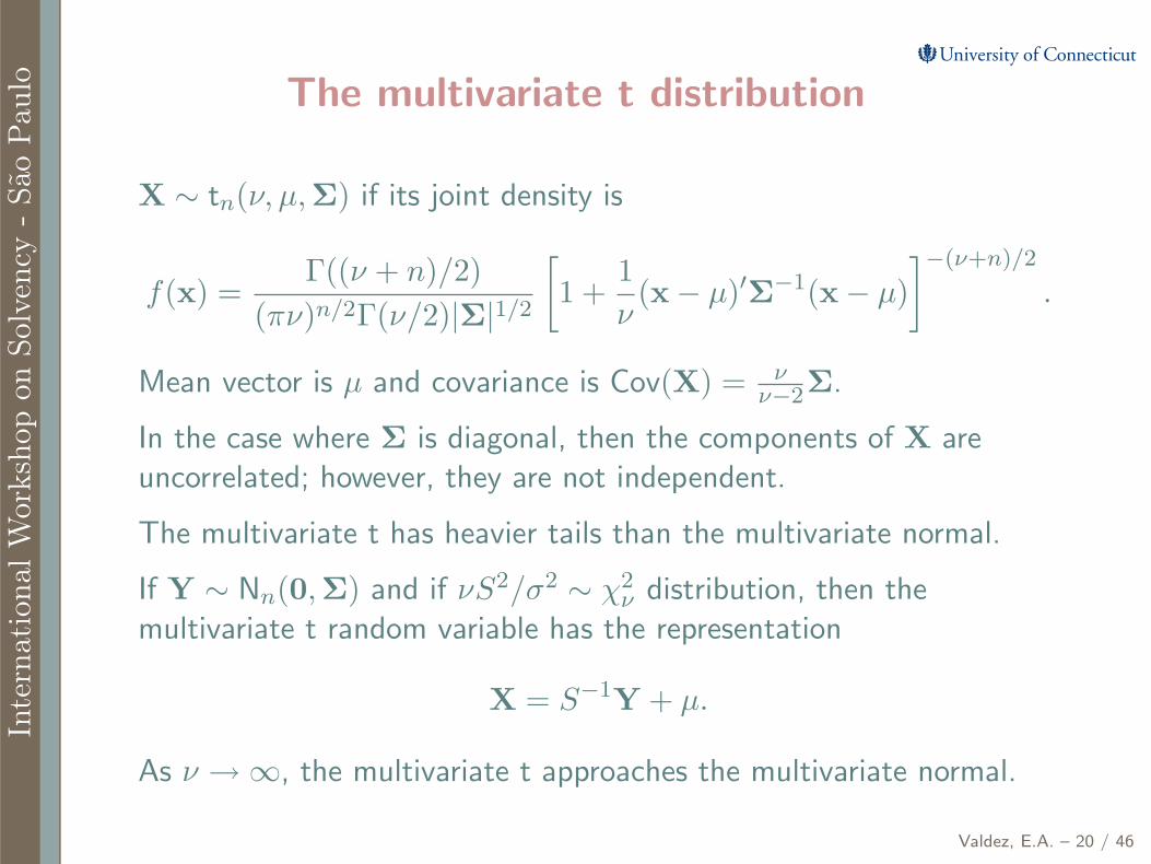
X ∼ tn(ν, µ,Σ) if its joint density is

f(x) =Γ((ν + n)/2)

(πν)n/2Γ(ν/2)|Σ|1/2

[

1 +1

ν(x − µ)′Σ−1(x − µ)

]−(ν+n)/2

.

Mean vector is µ and covariance is Cov(X) = νν−2Σ.

In the case where Σ is diagonal, then the components of X areuncorrelated; however, they are not independent.

The multivariate t has heavier tails than the multivariate normal.

If Y ∼ Nn(0,Σ) and if νS2/σ2 ∼ χ2ν distribution, then the

multivariate t random variable has the representation

X = S−1Y + µ.

As ν → ∞, the multivariate t approaches the multivariate normal.

Inte

rnati

onalW

ork

shop

on

Solv

ency

-São

Paulo Multivariate distribution function

Valdez, E.A. – 21 / 46

A function F : Rn → [0, 1] is a multivariate distribution function if it

satisfies:

• right-continuity;

• limxi→−∞ F (x1, . . . , xn) = 0 for i = 1, . . . , n;

• limxi→∞,∀i F (x1, . . . , xn) = 1; and

• rectangle inequality holds: for all (a1, . . . , an) and (b1, . . . , bn)with ai ≤ bi for i = 1, . . . , n, we have

2∑

i1=1

· · ·2

∑

in=1

(−1)i1+···+inF (x1i1 , . . . , xnin) ≥ 0,

where xi1 = ai and xi2 = bi.

Inte

rnati

onalW

ork

shop

on

Solv

ency

-São

Paulo Copula defined

Valdez, E.A. – 22 / 46

A copula C : [0, 1]n → [0, 1] is a multivariate distribution functionwhose univariate marginals are Uniform(0, 1).

Properties of a copula:

• C(u1, . . . , un) must be increasing in each component ui.

• C(u1, . . . , uk−1, 0, uk+1, . . . , un) = 0.

• C(1, . . . , 1, uk, 1, . . . , 1) = uk.

• the rectangle inequality leads us to

2∑

i1=1

· · ·2

∑

in=1

(−1)i1+···+inC(u1i1 , . . . , unin) ≥ 0

for all ui ∈ [0, 1], (a1, . . . , an) and (b1, . . . , bn) with ai ≤ bi,and ui1 = ai and ui2 = bi.

Inte

rnati

onalW

ork

shop

on

Solv

ency

-São

Paulo Sklar’s representation theorem

Valdez, E.A. – 23 / 46

Sklar (1959): There exists a copula function C such that

F (x1, . . . , xn) = C(F1(x1), . . . , Fn(xn))

where Fi is the marginal for Xi, i = 1, . . . , n.

Equivalently, we write

P(X1 ≤ x1, . . . , Xn ≤ xn) = C(P(X1 ≤ x1), . . . ,P(Xn ≤ xn)).

C need not be unique, but it is unique for continuous marginals.Else, C is uniquely determined on RanF1 × . . .× RanFn.

In the continuous case, this unique copula can be expressed as

C(u1, . . . , un) = F (F−11 (u1), . . . , F

−1n (un)),

where F−1i are the respective quantile functions.

Inte

rnati

onalW

ork

shop

on

Solv

ency

-São

Paulo Some examples

Valdez, E.A. – 24 / 46

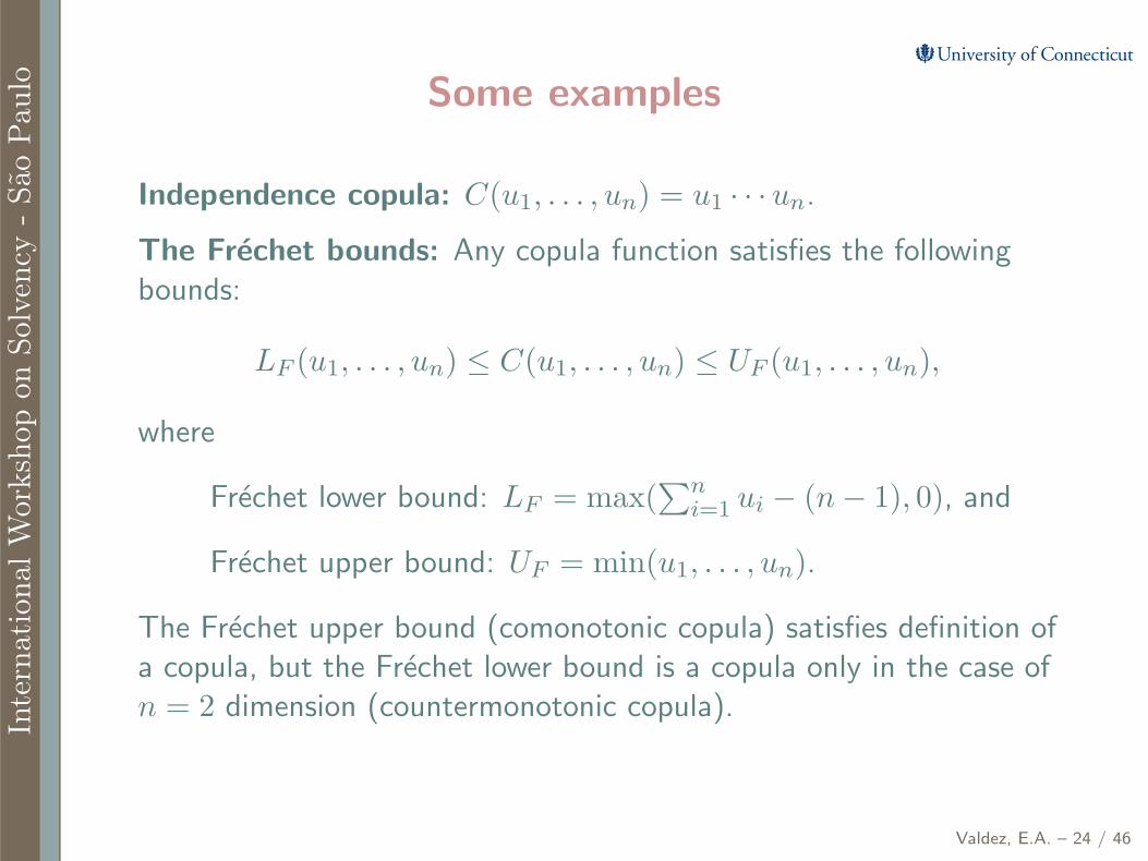
Independence copula: C(u1, . . . , un) = u1 · · ·un.

The Frechet bounds: Any copula function satisfies the followingbounds:

LF (u1, . . . , un) ≤ C(u1, . . . , un) ≤ UF (u1, . . . , un),

where

Frechet lower bound: LF = max(∑n

i=1 ui − (n− 1), 0), and

Frechet upper bound: UF = min(u1, . . . , un).

The Frechet upper bound (comonotonic copula) satisfies definition ofa copula, but the Frechet lower bound is a copula only in the case ofn = 2 dimension (countermonotonic copula).

Inte

rnati

onalW

ork

shop

on

Solv

ency

-São

Paulo The comonotonic copula

Valdez, E.A. – 25 / 46

Define the comonotonic copula CU = min(u1, . . . , un).

It can be shown that if F1, . . . , Fn are univariate marginal distributionfunctions, then CU is the distribution function of the random vector

(F−11 (U), . . . , F−1

n (U)),

where F−1i are the usual quantile functions.

Comonotonicity is indeed a very strong positive dependency structure- results in very strong positive comovements. The higher the value ofone component Xi, the higher the value of any other component Xj .

Studied by: Dhaene, et al. (2002a, 2002b). Very useful for findingbounds of functions of components of a random vector.

Inte

rnati

onalW

ork

shop

on

Solv

ency

-São

Paulo Invariance property

Valdez, E.A. – 26 / 46

Suppose random vector X has copula C and suppose T1, . . . , Tn arenon-decreasing continuous functions of X1, . . . , Xn , respectively.

The random vector defined by (T1(X1), . . . , Tn(Xn)) has the samecopula C.

The usefulness of this property can be illustrated in many ways. Ifyou have a copula describing joint distribution of insurance losses ofvarious types, and you decide the quantity of interest is atransformation (e.g. logarithm) of these losses, then the multivariatedistribution structure does not change.

Hence, the dependency structure is preserved. However, themarginals do change.

Inte

rnati

onalW

ork

shop

on

Solv

ency

-São

Paulo Examples of (implicit) copulas

Valdez, E.A. – 27 / 46

Normal copula:

CnR(u) = ΦR(Φ−1(u1), . . . ,Φ

−1(un)),

where Φ is the cdf of standard univariate normal, ΦR is the joint cdfof X ∼ Nn(0,R) with R, the correlation matrix.

The case where R = In results in independence, and R = Jn givescomonotonicity.

t copula:Cn

ν,R(u) = tν,R(t−1ν (u1), . . . , t

−1ν (un)),

where tν is the cdf of standard univariate t, tν,R is the joint cdf ofX ∼ tn(ν,0,R) with R, the correlation matrix.

The case where R = Jn gives comonotonicity, but R = In does notresult in independence.

Inte

rnati

onalW

ork

shop

on

Solv

ency

-São

Paulo Simulating normal and t copulas

Valdez, E.A. – 28 / 46

Although implicit in forms, these copulas are easy to simulate from.

Simulating from normal copula:

1. simulate X ∼ Nn(0,R);

2. set U = (Φ(X1), . . . ,Φ(Xn))′.

Simulating from t copula:

1. simulate X ∼ tn(ν,0,R);

2. set U = (tν(X1), . . . , tν(Xn))′.

Inte

rnati

onalW

ork

shop

on

Solv

ency

-São

Paulo Simulation - normal vs t copula

Valdez, E.A. – 29 / 46

0.0 0.2 0.4 0.6 0.8 1.0

0.00.2

0.40.6

0.81.0

Normal copula (rho=−0.90)

u1

u2

0.0 0.2 0.4 0.6 0.8 1.0

0.00.2

0.40.6

0.81.0

Normal copula (rho=0.20)

u1

u2

0.0 0.2 0.4 0.6 0.8 1.0

0.00.2

0.40.6

0.81.0

t3 copula (rho=−0.90)

u1

u2

0.0 0.2 0.4 0.6 0.8 1.0

0.00.2

0.40.6

0.81.0

t3 copula (rho=0.20)

u1

u2

Inte

rnati

onalW

ork

shop

on

Solv

ency

-São

Paulo Special class: Archimedean copulas

Valdez, E.A. – 30 / 46

C is an Archimedean if it has the form

C(u1, . . . , un) = ψ−1(ψ(u1) + · · · + ψ(un)),

for some function ψ (called the generator) satisfying:

• ψ(1) = 0;

• ψ is decreasing; and

• ψ is convex.

To ensure you get a legitimate copula for higher dimensions, ψ−1

must be completely monotonic, i.e. its derivatives alternate in signs.

An important source of Archimedean generators is the inverses of theLaplace transforms of distribution functions.

Feller (1971): A function ϕ on [0,∞] is the Laplace transform of acdf F if and only if ϕ is completely monotonic with ϕ(0) = 1.

Inte

rnati

onalW

ork

shop

on

Solv

ency

-São

Paulo Archimedean copulas and their generators

Valdez, E.A. – 31 / 46

Family Generator ψ(t) Range of α C(u)

Independence − log(t) nan∏

i=1ui

Clayton t−α − 1 α > 0

[

n∑

i=1u−α

i − n+ 1

]−1/α

Gumbel-Hougaard (− log t)α α ≥ 1 exp

−[

n∑

i=1(− log ui)

α

]1/α

Frank − log

(

e−αt − 1

e−α − 1

)

α > 0 − 1

αlog

1 +

n∏

i=1(e−αui − 1)

(e−α − 1)n−1

Inte

rnati

onalW

ork

shop

on

Solv

ency

-São

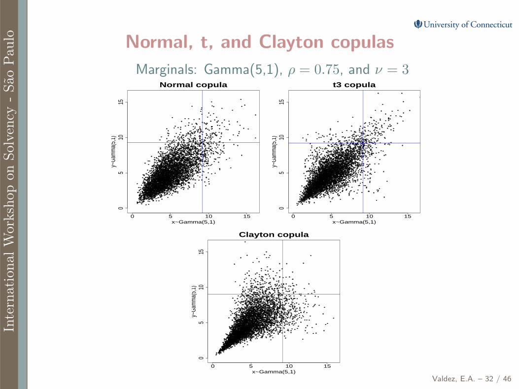
Paulo Normal, t, and Clayton copulas

Valdez, E.A. – 32 / 46

Marginals: Gamma(5,1), ρ = 0.75, and ν = 3

0 5 10 15

05

1015

Normal copula

x~Gamma(5,1)

y~Ga

mm

a(5,

1)

0 5 10 15

05

1015

t3 copula

x~Gamma(5,1)

y~Ga

mm

a(5,

1)

0 5 10 15

05

1015

Clayton copula

x~Gamma(5,1)

y~Ga

mm

a(5,

1)

Inte

rnati

onalW

ork

shop

on

Solv

ency

-São

Paulo Calibrating copula models

Valdez, E.A. – 33 / 46

In demonstrating how to calibrate copula models, we considerempirical data with:

• Danish fire data provided by Mette Rytgaard.

• The data consists of 2,167 fire losses in Denmark for the period1980-1990.

• The loss amounts vary according to:

• buildings X1

• contents X2

• loss of profits X3

• This same dataset has been used by Blum, Dias and Embrechts(2002), “The ART of Dependence Modelling”, appearing inAlternative Risk Strategies, ed. M. Lane.

Inte

rnati

onalW

ork

shop

on

Solv

ency

-São

Paulo The first 10 observed values

Valdez, E.A. – 34 / 46

building contents loss of profit total

1.09809663 0.58565150 0.00000000 1.6837481.75695461 0.33674960 0.00000000 2.0937041.73258126 0.00000000 0.00000000 1.7325810.00000000 1.30537600 0.47437775 1.7797541.24450952 3.36749600 0.00000000 4.6120064.45203953 4.27323400 0.00000000 8.7252742.49487555 3.54319200 1.86090776 7.8989750.77568960 0.99311710 0.43923865 2.2080450.81259151 0.67349930 0.00000000 1.4860912.37157394 0.16837480 0.25622255 2.796171

Inte

rnati

onalW

ork

shop

on

Solv

ency

-São

Paulo Some summary statistics

Valdez, E.A. – 35 / 46

type of lossbuilding contents loss of profit total

zero counts 177 488 1,551(non-zero) count 1,990 1,679 616 2,167mean 1,986,679 1,701,778 851,799 3,385,088median 1,320,132 575,699 266,193 1,778,154std dev 4,514,998 5,347,536 2,947,029 8,507,451minimum 23,191 825 4,084 1,000,000maximum 152,413,209 132,013,200 61,932,650 263,250,32425th percentile 966,175 290,004 100,111 1,321,11875th percentile 1,978,604 1,446,480 679,293 2,967,023

Inte

rnati

onalW

ork

shop

on

Solv

ency

-São

Paulo Marginal density plots

Valdez, E.A. – 36 / 46

5 10 15 20

0.00.2

0.40.6

0.8

Densities of logarithm of losses

log of loss

Densi

ty

building

contents

profits

Inte

rnati

onalW

ork

shop

on

Solv

ency

-São

Paulo Q-Q plots of the logarithms

Valdez, E.A. – 37 / 46

−3 −2 −1 0 1 2 3

−4−2

02

4

building

Theoretical Quantiles

Sam

ple Q

uant

iles

−3 −2 −1 0 1 2 3

−6−4

−20

24

contents

Theoretical Quantiles

Sam

ple Q

uant

iles

−3 −2 −1 0 1 2 3

−4−2

02

4

contents

Theoretical Quantiles

Sam

ple Q

uant

iles

Inte

rnati

onalW

ork

shop

on

Solv

ency

-São

Paulo Fitting the marginals

Valdez, E.A. – 38 / 46

To accomodate the large number of zeroes in each type of loss, weuse a mixture model of the form:

fk(x) =

pk, for x = 0(1 − pk)fLN,k(x), for x > 0

,

where k = 1, 2, 3 refers to the building, contents, and profits,respectively.

LN refers to the log-normal distribution with parameters µ and σ.

It is also easy to prove that the marginal CDF for the mixture is:

Fk(x) = pk + (1 − pk)FLN,k(x), for k = 1, 2, 3.

Inte

rnati

onalW

ork

shop

on

Solv

ency

-São

Paulo Marginal parameter estimates

Valdez, E.A. – 39 / 46

Estimation used: Inference for Margins (IFM) method

Parameter Building (X1) Contents (X2) Profits (X3)

p 0.0817 0.2253 0.7156(s.e.) (0.0059) (0.0090) (0.0097)µ 0.3384 -0.4257 -1.2802

(s.e.) (0.0167) (0.0310) (0.0570)σ 0.7438 1.2705 1.4153

(s.e.) (0.0118) (0.0219) (0.0403)

Inte

rnati

onalW

ork

shop

on

Solv

ency

-São

Paulo Copula dependence parameter estimates

Valdez, E.A. – 40 / 46

Parameter Clayton copula Normal copula t-copula

α 0.0162(s.e.) (0.0128)

ρBC 0.3218 0.3194(s.e.) (0.0056) (0.0017)ρBP 0.2862 0.3005(s.e.) (0.0022) (0.0059)ρCP 0.2825 0.2864(s.e.) (0.0089) (0.0073)ν 2.9974

(s.e.) (0.1736)

log-likelihood -8,291.897 -8,188.390 -8,235.523numb. of parms. 1 3 4

AIC 16,585.79 16,382.78 16,479.05

Inte

rnati

onalW

ork

shop

on

Solv

ency

-São

Paulo Approaches to aggregating risks

Valdez, E.A. – 41 / 46

• Standard methodology - based on the following assumptions:

(i) X = (X1, . . . , Xn)′ follows a multivariate normal withmean µ = (µ1, . . . , µn)′ and covariance Σ = (σij); and

(ii) The risk measure used is the quantile risk measure or VaR.

• Extension to the standard methodology - based on the followingassumptions:

(i) Each Xi belongs to a location-scale family of distributions:

Xi = µi + σiZ, for i = 1, . . . , n.

(ii) S also belongs to same location-scale family:S = µS + σSZ; and

(iii) Risk measure used is conditional tail expectation or TVaR.

• Numerical simulations with copulas.

Inte

rnati

onalW

ork

shop

on

Solv

ency

-São

Paulo The standard methodology

Valdez, E.A. – 42 / 46

S has a normal distribution with mean E(S) =∑n

i=1 µi and varianceVar(S) = 1

′Σ1, where 1 = (1, 1, . . . , 1)′.

Thus, we haveSCRS = VaRq(S) − E(S),

where, using the property of normal distribution, we have

VaRq(S) = Φ−1(q)σS + E(S),

and hence,

SCRS = Φ−1(q)σS = Φ−1(q)√

Var(S) = Φ−1(q)√

1′Σ1.

Φ−1 denotes the quantile function of a standard normal and σS is thestandard deviation of S.

Inte

rnati

onalW

ork

shop

on

Solv

ency

-São

Paulo The standard methodology - continued

Valdez, E.A. – 43 / 46

Note that

1′Σ1 =

n∑

i=1

n∑

j=1

Cov(Xi, Xj) =n

∑

i=1

n∑

j=1

σiσjρij

=1

[Φ−1(q)]2

n∑

i=1

n∑

j=1

SCRiSCRjρij =1

[Φ−1(q)]2SCR′

Σ SCR,

whereSCR = (SCRX1

, . . . ,SCRXn)′,

the vector of stand-alone solvency capitals SCRXifor each risk i.

This proof has appeared in Dhaene (2005). It immediately followsthat

SCRS =√

SCR′Σ SCR.

The stand-alone capitals can indeed be written as

SCRXi= Φ−1(q)σXi

= Φ−1(q)√

Var(Xi).

Inte

rnati

onalW

ork

shop

on

Solv

ency

-São

Paulo Extension to the standard methodology

Valdez, E.A. – 44 / 46

For stand-alone losses Xi, we have

TVaRq(Xi) = E(Xi|Xi > VaRq(Xi))

= µi + σiE(Z|Z > VaRq(Z))

= µi + σiTVaRq(Z).

Similarly, we have TVaRq(S) = µS + σSTVaRq(Z).

From here, we find that

1′Σ1 =

1

[TVaRq(Z)]2

n∑

i=1

n∑

j=1

(TVaRq(Xi) − µi)ρij(TVaRq(Xj) − µj)

=1

[TVaRq(Z)]2(TVaRq(X) − µ)′Σ(TVaRq(X) − µ).

where TVaRq(X) = (TVaRq(X1), . . . ,TVaRq(Xn))′, the vector ofstand-alone solvency capitals TVaRq(Xi) for each risk i.

Inte

rnati

onalW

ork

shop

on

Solv

ency

-São

Paulo Extension - continued

Valdez, E.A. – 45 / 46

It follows that

SCRS = µS +√

(TVaRq(X) − µ)′ Σ (TVaRq(X) − µ).

A similar form to the standard methodology can be found in this case:

SCRS = µS +√

SCR′Σ SCR.

Indeed, Dhaene (2005) provides a further extension to the class ofdistortion risk measures for which the Tail VaR is a special case.

This class of risk measures was introduced by Wang (1996).

Inte

rnati

onalW

ork

shop

on

Solv

ency

-São

Paulo Some useful references

Valdez, E.A. – 46 / 46

Dhaene, J., Goovaerts, M.J., Lundin, M. and S. Vanduffel, 2005,Aggregating economic capital, Belgian Actuarial Bulletin, 5: 14-25.

Frees, E.W. and E.A. Valdez, 1998, Understanding relationships usingcopulas, North American Actuarial Journal, 2: 1-25.

Joe, H., 1997, Multivariate models and dependence concepts, NewYork: Chapman & Hall.

McNeil, A.J., Frey, R. and P. Embrechts, 2005, Quantitative risk

management: concepts, techniques and tools, Princeton, N.J.:Princeton University Press.

McNeil, A.J., 2007, Lecture slides on modelling dependent financialrisks: non-gaussian models and copulas, Maresias, Brazil.

Sandstrom, A., 2006, Solvency: models, assessment and regulation,Boca Raton, FL: Chapman & Hall/CRC.