Models of complexity growthand random quantum circuits

Nick Hunter-Jones

Perimeter Institute

June 25, 2019Yukawa Institute for Theoretical Physics

Based on:[Kueng, NHJ, Chemissany, Brandao, Preskill], 1907.hopefully soon[NHJ], 1905.12053

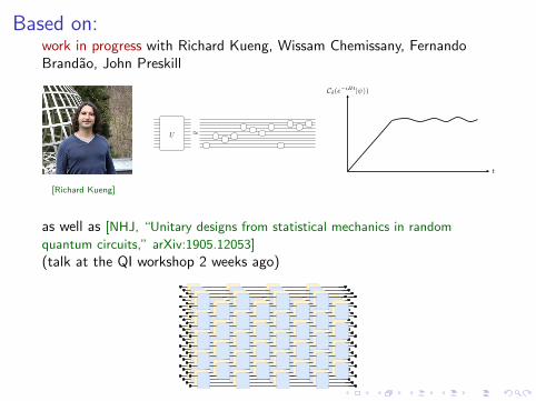
Based on:work in progress with Richard Kueng, Wissam Chemissany, FernandoBrandao, John Preskill

U ⇡

1

C�(e�iHt| i)

t

[Richard Kueng]

as well as [NHJ, “Unitary designs from statistical mechanics in random

quantum circuits,” arXiv:1905.12053]

(talk at the QI workshop 2 weeks ago)

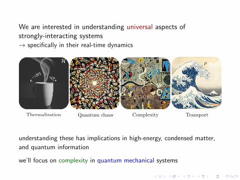
We are interested in understanding universal aspects ofstrongly-interacting systems→ specifically in their real-time dynamics

Thermalization Transport

⇢

Quantum chaos

R2

Complexity

C�(| i)

understanding these has implications in high-energy, condensed matter,

and quantum information

we’ll focus on complexity in quantum mechanical systems

Complexitysome intuition

Complexity is a somewhat intuitive notion

The traditional definition involves building a circuit with gatesdrawn from a universal gate set, which implements the state orunitary to within some tolerance

U ≈

We are interested in the minimal size of a circuit that achieves this

Complexitya panoply of references

we’ve heard a lot about complexity growth already in this workshope.g. talks by Rob Myers, Vijay Balasubramanian, and Thom Bohdanowicz;

in talks later today/this week by Bartek Czech, Gabor Sarosi, Shira Chapman; and in many posters

and much progress has been made in studying complexity growthin holographic systems[Susskind], [Stanford, Susskind], [Brown, Roberts, Susskind, Swingle, Zhao], [Susskind, Zhao], [Couch, Fischler,

Nguyen], [Carmi, Myers, Rath], [Brown, Susskind], [Caputa, Magan], [Alishahiha], [Chapman, Marrochio, Myers],

[Carmi, Chapman, Marrochio, Myers, Sugishita], [Caputa, Kundu, Miyaji, Takayanagi, Watanabe], [Brown,

Susskind, Zhao], [Agon, Headrick, Swingle], . . .

as well as extending definitions to understand a notion ofcomplexity in QFT[Chapman, Heller, Marrochio, Pastawski], [Jefferson, Myers], [Hackl, Myers], [Yang], [Chapman, Eisert, Hackl,

Heller, Jefferson, Marrochio, Myers], [Guo, Hernandez, Myers, Ruan], . . .

Complexitysome expectations

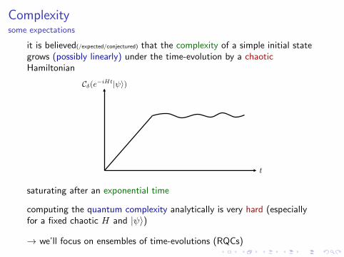
it is believed(/expected/conjectured) that the complexity of a simple initial stategrows (possibly linearly) under the time-evolution by a chaoticHamiltonian

C�(e�iHt| i)

t

saturating after an exponential time

computing the quantum complexity analytically is very hard (especiallyfor a fixed chaotic H and |ψ〉)

→ we’ll focus on ensembles of time-evolutions (RQCs)

Our goal

Consider random quantum circuits, a solvable model of chaotic dynamics

we take local RQCs on n qudits of local dimension q, with gates drawnrandomly from a universal gate set G

t

and try to derive exact results for the growth of complexity

Overview

I Define complexity

I Complexity by design

I Complexity in local random circuits

I Solving random circuits

I (complexity from measurements)

State complexitymore serious version

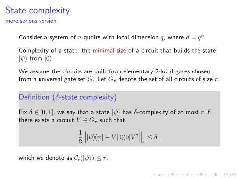
Consider a system of n qudits with local dimension q, where d = qn

Complexity of a state: the minimal size of a circuit that builds the state|ψ〉 from |0〉

We assume the circuits are built from elementary 2-local gates chosenfrom a universal gate set G. Let Gr denote the set of all circuits of size r.

Definition (δ-state complexity)

Fix δ ∈ [0, 1], we say that a state |ψ〉 has δ-complexity of at most r ifthere exists a circuit V ∈ Gr such that

1

2

∥∥∥|ψ〉〈ψ| − V |0〉〈0|V †∥∥∥1≤ δ ,

which we denote as Cδ(|ψ〉) ≤ r.

Unitary complexitymore serious version

Consider a system of n qudits with local dimension q, where d = qn

Complexity of a unitary: the minimal size of a circuit, built from a 2-localgates from G, that approximates the unitary U

Definition (δ-unitary complexity)

We say that a unitary U ∈ U(d) has δ-complexity of at most r if thereexists a circuit V ∈ Gr such that

1

2

∥∥U − V∥∥� ≤ δ ,where U = U(ρ)U† and V = V (ρ)V † ,

which we denote as Cδ(U) ≤ r.

Complexity by design

We start with some general statements about the complexity ofunitary k-designs

related ideas were presented in [Roberts, Yoshida] relating the frame potential

to the average complexity of an ensemble

But first, we need to define the notion of a unitary design

Unitary k-designs

Haar: (unique L/R invariant) measure on the unitary group U(d)

The k-fold channel, with respect to the Haar measure, of an operator Oacting on H⊗k is

Φ(k)Haar(O) ≡

∫Haar

dU U⊗k(O)U†⊗k

For an ensemble of unitaries E = {pi, Ui}, the k-fold channel of anoperator O acting on H⊗k is

Φ(k)E (O) ≡

∑i

piU⊗ki (O)U†i

⊗k

An ensemble of unitaries E is an exact k-design if

Φ(k)E (O) = Φ

(k)Haar(O)

e.g. k = 1 and Paulis, k = 2, 3 and the Clifford group

Unitary k-designs

Haar: (unique L/R invariant) measure on the unitary group U(d)

k-fold channel: Φ(k)E (O) ≡∑i piU

⊗ki (O)U †i

⊗k

exact k-design: Φ(k)E (O) = Φ

(k)Haar(O)

but for general k, few exact constructions are known

Definition (Approximate k-design)

For ε > 0, an ensemble E is an ε-approximate k-design if the k-foldchannel obeys ∥∥∥Φ

(k)E − Φ

(k)Haar

∥∥∥�≤ ε

→ designs are powerful

Intuition for k-designs(eschewing rigor)

How random is the time-evolution of a system compared to the fullunitary group U(d)?

Consider an ensemble of time-evolutions at a fixed time t: Et = {Ut}e.g. RQCs, Brownian circuits, or {e−iHt, H ∈ EH} generated by

disordered Hamiltonians

U(d)

1•Ut

quantify randomness:when does Et form a k-design?(approximating moments of U(d))

Complexity by designan exercise in enumeration

Consider a discrete approximate unitary design E = {pi, Ui}.

Can we say anything about the complexity of Ui’s?

The structure of a design is sufficiently restrictive, can count thenumber of unitaries of a specific complexity

Theorem (Complexity for unitary designs)

For δ > 0, an ε-approximate unitary k-design contains at least

M ≥ d2k

k!

1

(1 + ε′)− nr|G|r

(1− δ2)k

unitaries U with Cδ(U) > r.

This is essentially ≈ (d2/k)k for r . kn (exp growth in design k)

Random quantum circuits

Consider G-local RQCs on n qudits of local dimension q, evolved withstaggered layers of 2-site unitaries, each drawn randomly from a universalgate set G

t

where evolution to time t is given by Ut = U (t) . . . U (1)

RQCs and randomness

Now we need a powerful result from [Brandao, Harrow, Horodecki]

Theorem (G-local random circuits form approximate designs)

For ε > 0, the set of all G-local random quantum circuits of size Tforms an ε-approximate unitary k-design if

T ≥ cndlog ke2k10(n+ log(1/ε))

where c is a (potentially large) constant depending on the universalgate set G.

Less rigorous version: RQCs of size T ∼ n2k10 form k-designs

Complexity by designcurbing collisions

Now we can combine these two results to say something about thecomplexity of states generated by G-local random circuits

Fix some initial state |ψ0〉, and consider the set of states generated byG-local RQCs: {Ui |ψ0〉 , Ui ∈ EG-local RQC}

Obviously, at early times: Cδ(|ψ〉) ≈ T

but we must account for collisions: U1 |ψ0〉 ≈ U2 |ψ0〉

and collisions must dominate at exponential times as the complexitysaturates

but the definition of an ε-approximate design restricts the number ofpotential collisions→ allows us to count the # of distinct states

Complexity by designcurbing collisions

Now we can combine these two results to say something about thecomplexity of states generated by G-local random circuits

Fix some initial state |ψ0〉, and consider the set of states generated byG-local RQCs: {Ui |ψ0〉 , Ui ∈ EG-local RQC}

For r ≤√d, G-local RQCs of size T , where T ≥ c n2(r/n)10, generate at

leastM & c′er logn

distinct states with Cδ(|ψ〉) > r.

This establishes a polynomial relation between the growth of complexityand size of the circuit up to r ≤

√d

→ but what we really want is linear growth

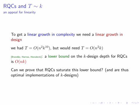
RQCs and T ∼ kan appeal for linearity

To get a linear growth in complexity we need a linear growth indesign

we had T = O(n2k10), but would need T = O(n2k)

[Brandao, Harrow, Horodecki]: a lower bound on the k-design depth for RQCsis O(nk)

Can we prove that RQCs saturate this lower bound? (and are thusoptimal implementations of k-designs)

k-designs from stat-mech in RQCs

I’ll now briefly summarize the result mentioned two weeks ago

using an exact stat-mech mapping, we can show that RQCs formk-designs in O(nk) depth in the limit of large local dimension

this was for local Haar-random gates, but we believe it shouldextend to G-local circuits with any local dimension q

Random quantum circuits

Consider local RQCs on n qudits of local dimension q, evolved withstaggered layers of 2-site unitaries, each drawn randomly from the Haarmeasure on U(q2)

t

where evolution to time t is given by Ut = U (t) . . . U (1)

Study the convergence of random quantum circuits to unitary k-designs,i.e. depth where we start approximating moments of the unitary group

Our approach

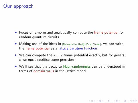
I Focus on 2-norm and analytically compute the frame potential forrandom quantum circuits

I Making use of the ideas in [Nahum, Vijay, Haah], [Zhou, Nahum], we can writethe frame potential as a lattice partition function

I We can compute the k = 2 frame potential exactly, but for generalk we must sacrifice some precision

I We’ll see that the decay to Haar-randomness can be understood interms of domain walls in the lattice model

Frame potential

The frame potential is a tractable measure of Haar randomness,defined for an ensemble of unitaries E as [Gross, Audenaert, Eisert], [Scott]

k-th frame potential : F (k)E =

∫U,V ∈E

dUdV∣∣Tr(U †V )

∣∣2kFor any ensemble E , the frame potential is lower bounded as

F (k)E ≥ F (k)

Haar and F (k)Haar = k! (for k ≤ d)

with = if and only if E is a k-design.

Related to ε-approximate k-design as∥∥∥Φ(k)E − Φ

(k)Haar

∥∥∥2�≤ d2k

(F (k)E −F

(k)Haar

)

Frame potential for RQCs

The goal is to compute the FP for RQCs evolved to time t:

F (k)RQC =

∫Ut,Vt∈RQC

dUdV∣∣Tr(U†t Vt)

∣∣2kConsider the k-th moments of RQCs, k copies of the circuit and itsconjugate:

Lattice mappings for RQCs

Haar averaging the 2-site unitaries allows us to exactly write the framepotential as a partition function on a triangular lattice.

The result is then that we can write the k-th frame potential as

F (k)RQC =

∑{σ}

∏/

Jσ1σ2σ3

=∑{σ}

with σ ∈ Sk, width ng = bn/2c, depth 2(t− 1), and pbc in time.

The plaquettes are functions of three σ ∈ Sk, written explicitly as

Jσ1σ2σ3

= σ1

σ2

σ3

=∑τ∈Sk

Wg(σ−11 τ, q2)q`(τ−1σ2)q`(τ

−1σ3) .

Lattice mappings for RQCs

Haar averaging the 2-site unitaries allows us to exactly write the framepotential as a partition function on a triangular lattice.

The result is then that we can write the k-th frame potential as

F (k)RQC =

∑{σ}

∏/

Jσ1σ2σ3

=∑{σ}

with σ ∈ Sk, width ng = bn/2c, depth 2(t− 1), and pbc in time.

We can show that Jσσσ = 1, and thus the minimal Haar value of theframe potential comes from the k! ground states of the lattice model

F (k)RQC = k! + . . .

RQC domain walls

all non-zero contributions to F (k)RQC are domain walls

(which must wrap the circuit)

e.g. for k = 2 we have

a single domain wallconfiguration:

a double domain wallconfiguration:

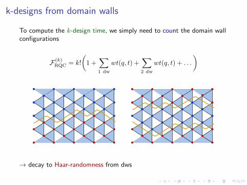
k-designs from domain walls

To compute the k-design time, we simply need to count the domain wallconfigurations

F (k)RQC = k!

(1 +

∑1 dw

wt(q, t) +∑2 dw

wt(q, t) + . . .

)

→ decay to Haar-randomness from dws

RQC 2-design time

We have the k = 2 frame potential for random circuits

F (2)RQC ≤ 2

(1 +

(2q

q2 + 1

)2(t−1))ng−1

and recalling that∥∥Φ

(2)RQC − Φ

(2)Haar

∥∥2� ≤ d4

(F (2)

RQC −F(2)Haar

),

the circuit depth at which we form an ε-approximate 2-design is then

t2 ≥ C(2n log q + log n+ log 1/ε

)with C =

(log

q2 + 1

2q

)−1and where for q = 2 we have t2 ≈ 6.2n, and in the limit q →∞ we findt2 ≈ 2n

k-designs in RQCs

For general k, we then have the contribution from the ground states andsingle domain wall sector, plus higher order contributions

F (k)RQC ≤ k!

(1 + (ng − 1)

(k

2

)(2(t− 1)

t− 1

)( q

q2 + 1

)2(t−1)+ . . .

)

Moreover, the multi-domain wall terms are heavily suppressed and higherorder interactions are subleading in 1/q as

∼ 1

qp

In the large q limit, the single domain wall sector gives the ε-approximatek-design time: tk ≥ C(2nk log q + k log k + log(1/ε)), which is

tk = O(nk)

k-designs in RQCs

For general k, we then have the contribution from the ground states andsingle domain wall sector, plus higher order contributions

F (k)RQC ≤ k!

(1 + (ng − 1)

(k

2

)(2(t− 1)

t− 1

)( q

q2 + 1

)2(t−1)+ . . .

)

Moreover, the multi-domain wall terms are heavily suppressed and higherorder interactions are subleading in 1/q as

∼ 1

qp

In the large q limit, the single domain wall sector gives the ε-approximatek-design time: tk ≥ C(2nk log q + k log k + log(1/ε)), which is

tk = O(nk)

k-designs from stat-mech

RQCs form k-designs in O(nk) depth

we showed this in the large q limit, but this limit is likely not necessary

Conjecture: The single domain wall sector of the lattice partitionfunction dominates the multi-domain wall sectors for highermoments k and any local dimension q.

As the lower bound on the design depth is O(nk), RQCs are thenoptimal implementations of randomness

Back to complexity

We’ll now end on a much more speculative note

If this result holds for G-local random circuits, and for any localdimension q, then the circuits of size T = O(n2k) form approx unitaryk-designs

Therefore, G-local RQCs of size T generate at least M ≥ (d/k)k distinctstates with complexity Cδ(|ψ〉) ≈ T . For k ≤

√d, we have

M & eT logn

This would then realize a conjecture by [Brown, Susskind] in an explicitexample:

the # of states with Cδ(UT |ψ0〉) ≈ T , generated by time-evolution totime T (in this case RQCs of size T ), scales exponentially in T

Future science

I Can we prove anything about Cδ(e−iHt |ψ〉) for a fixedHamiltonian?

I Can we rigorously bound the higher order terms in F (k)RQC at

small q? and then extend the result to G-local RQCs

I Explore the implications of an operational definition ofcomplexity (in terms of a distinguishing measurement). Moresuited for holography?

Thanks!

(ご清聴ありがとうございました)