Embed Size (px)
Citation preview

Models of collective inference
Laurent Massoulié (Microsoft Research-Inria Joint Centre)Mesrob I. Ohannessian (University of California, San Diego)Alexandre Proutière (KTH Royal Institute of Technology)Kuang Xu (Stanford)

Outline Spreading news to interested usersHow to jointly achieve news
-categorization by users, and -dissemination to interested users
[LM, M.Ohanessian, A. Proutière, Sigmetrics 15]
Information-processing systemsTreatment of inference tasks by pool of agents with limited capacities (ex: crowdsourcing)
[LM, K. Xu 15]
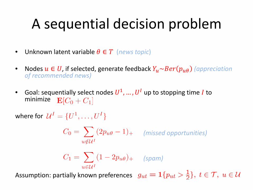
A sequential decision problem
• Unknown latent variable 𝜃𝜃 ∈ 𝑇𝑇 (news topic)
• Nodes 𝑢𝑢 ∈ 𝑈𝑈, if selected, generate feedback 𝑌𝑌𝑢𝑢~𝐵𝐵𝐵𝐵𝐵𝐵 𝑝𝑝𝑢𝑢𝑢𝑢 (appreciationof recommended news)
• Goal: sequentially select nodes 𝑈𝑈1, … ,𝑈𝑈𝐼𝐼 up to stopping time 𝐼𝐼 to minimize
where for
(missed opportunities)
(spam)
Assumption: partially known preferences

Related Work
• Multi-Armed Bandits (MAB):– Contextual [Li et al. 2010]– Infinitely many arms [Berry et al. 1997]– Secretary problem [Ferguson 1989]– Best arm identification [Kaufmann et al. 2014]
• Distinguishing features:– Partial information on parameters– Finitely many, exhaustible arms– Stopping time, trades off two regrets– Find all good arms, not the best
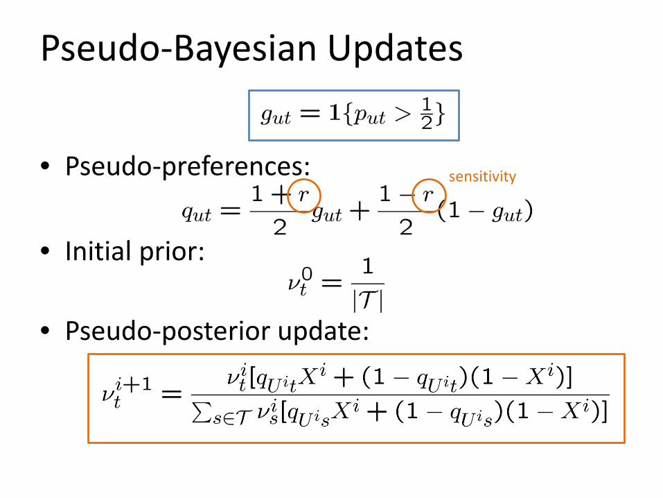
Pseudo-Bayesian Updates
• Pseudo-preferences:
• Initial prior:
• Pseudo-posterior update:
sensitivity

Greedy-Bayes Algorithm
– Initialize pseudo-preferences and prior– At each step i
• Make greedy selection
• Based on response ,update pseudo-posterior
• Stop ifthreshold
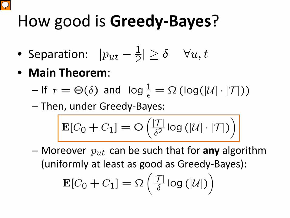
How good is Greedy-Bayes?
• Separation:• Main Theorem:
– If and ,– Then, under Greedy-Bayes:
– Moreover can be such that for any algorithm (uniformly at least as good as Greedy-Bayes):

The tool: Bernstein’s inequality for martingales
[Freedman’75]
Martingale 𝑀𝑀𝑖𝑖𝑖𝑖≥1 with compensator 𝑀𝑀 𝑖𝑖 and
increments bounded by 𝐵𝐵 satisfies for any stoppingtime 𝐼𝐼

Proof sketchbound on spamming regret 𝐶𝐶1
Key quantity:
Goal:

Proof sketchbound on spamming regret 𝐶𝐶1
Martingale analysis of 𝑅𝑅𝑖𝑖 : 𝑅𝑅𝑖𝑖= 𝐴𝐴𝑖𝑖 + 𝑀𝑀𝑖𝑖 where 𝑀𝑀𝑖𝑖 martingale with increments bounded by O 𝛿𝛿 , and for some �𝑍𝑍𝑖𝑖 ≥ 𝑍𝑍𝑖𝑖:
Hence:
then apply Freedman’s inequality

Lower regret with extra structure• Topic that many like who dislike other topics
(*)
• Theorem: Under (*), if then for topic 𝜃𝜃
Greedy-Bayes has regret
• Moreover can be such that
for any algorithm (uniformly at least as good as Greedy-Bayes)
• Other conditions give log|T| instead of |T|
Constant in |U|

Greedy-Bayes Algorithm
• Given matrix :– Initialize pseudo-preferences and prior.– At each step i
• Make a greedy selection:
• Observe the response • Update the pseudo-posterior:
– Stop if:
Thompson sampling Algorithm
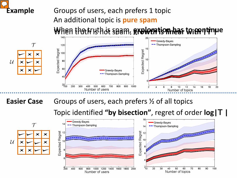
When truth is not spam, growth is linear with |T |
Example Groups of users, each prefers 1 topic
Easier Case Groups of users, each prefers ½ of all topics
When the truth is spam, exploration has to continue
Topic identified “by bisection”, regret of order log|T |
An additional topic is pure spam

Summary
• Push-based news dissemination• Extension of multi-armed bandit ideas• Greedy-Bayes algorithm
– Simple yet provably order-optimal– Robust, uses only partial preference information– Adaptive to structure
• Implications– Benchmark for push-pull decentralization– Importance of leveraging negative feedback

Open questions• Is there a simple characterization in terms of
of the optimal regret?
• Is Greedy-Bayes (or Thompson Sampling) order-optimal under more general conditions?
partial answers:Toy examples where greed fails to probe highly informative nodes with high expected contribution to regretHope for somewhat general conditions under which GreedyBayes performs near-bisection

Systems that perform inference/categorization tasks, based on queries to resource-limited agents
Crowd sourcing Human experts Machine learning (e.g., clustering) Cloud clusters Medical lab diagnostics Specialized lab machines
Output based on large number of noisy inspections
Goal: identify efficient processing which uses minimum amount of resources
Capacity of Information Processing Systems
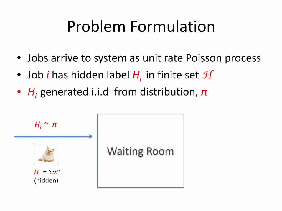
Problem Formulation
• Jobs arrive to system as unit rate Poisson process• Job i has hidden label Hi in finite set H• Hi generated i.i.d from distribution, π
Waiting Room
Hi = ‘cat’(hidden)
Hi ~ π

Problem Formulation
• Goal: output estimated label, H’i, s.t.
Waiting Room
Hi = ‘cat’(hidden)
Hi ~ π
if H’i = ‘cat’
if H’i = ‘dog’

System resources• m experts of which rk fraction is type-k
• Type-k expert when inspecting type h- job produces random response X:
for distributions { f(h,k,*) } assumed known
• Single job inspection occupies an expert for time Exp(1)
Based on inspection history (x1, k1), (x2,k2), …. (xn,kn), Could tag job with ML estimator

Learning System
Waiting Room
Hi = ‘cat’(hidden)
Hi ~ π
H’i
1 1 2 2 2 K K
m*r2
(x,1)

Inspection Policy
• An inspection policy, ϕ, decides
1. Which experts to inspect which jobs - based on past history
2. When a job will be allowed to depart from the system
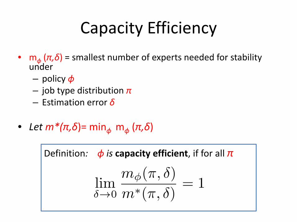
Definition: ϕ is capacity efficient, if for all π
Capacity Efficiency• mϕ (π,δ) = smallest number of experts needed for stability
under– policy ϕ– job type distribution π– Estimation error δ
• Let m*(π,δ)= minϕ mϕ (π,δ)

Main Result
Theorem
1. There exists a capacity efficient policy ϕ, s.t.
2. The policy ϕ does not require knowledge of π

Main Result (cont.)
• Makes no restrictions on response distributions {f(h,k,*)}
• Distribution π may be unknown and change over time
advantageous to have– Upper bound independent of π– π-oblivious inspection policy
• Constant c is explicit (but messy), and is proportional to – 1/ (mink rk)– total number of labels– Ratio between KL-divergences among distributions of inspection
results

Related Work• Classical sequential hypothesis testing
– Single expert by Wald 1945, Multi-expert model by Chernoff 1959
– Costs measured by sample complexity– Does not involve finite resource constraint or simultaneous
processing of multiple jobs
• Max-Weight policy in network resource allocation– Policy contains a variant of Max-Weight policy as a sub-
module– Need to work with approximate labels and resolve
synchronicity issues

Proof OutlineMain Steps:
1. Translate estimation accuracy into service requirements
2. Design processing architecture to balance contention for services among different job labels
Technical ingredients:
1. ``Min-weight” adaptive policy using noisy job labels2. Fluid model to prove stability over multiple stages

From Statistics to Services• Consider single job i• Suppose i leaves system upon receiving N inspections, with history
• Write
• Define likelihood ratio:

From Statistics to Services
Lemma (Sufficiency of a Likelihood Ratio Test)Define event
Then
Lemma (Necessity)
If decision rule yields error < δ then it must be that

From Statistics to Services• For true job type Hi=h , “service requirement” of job i: For all 𝑙𝑙 ≠ ℎ need to inspect job i until S(h,l) reaches ln(1/δ)
Job i arrives with vector of “workloads” with initial level = ln(1/δ) for all coordinates 𝑙𝑙 ≠ ℎ
• Job of true type h when inspected by type-k expertreceives ``service”
Expected service amount: KL-divergence

Lower bound on performance• If we knew true labels of all jobs and label distribution π, we would
need m as large as solution �𝑚𝑚(𝜋𝜋, 𝛿𝛿) of LP:
Where nh,k : Number of inspections of h-labeled job by type-k expert
Solution of LP, �𝑚𝑚 𝜋𝜋, 𝛿𝛿 = C ln(1𝛿𝛿
) : lower bound on optimal capacity requirement

Processing Architecture
• Preparation stage: crude estimates of types from randomized inspections
• Adaptive stage: use crude estimates to ``boot-strap’’ adaptiveallocation policy for bulk of inspections and refinement of type estimates
– Generate approximately optimal nh,k as in LP
• Residual stage: fix poorly learned labels from AdaptiveStage with randomized inspections
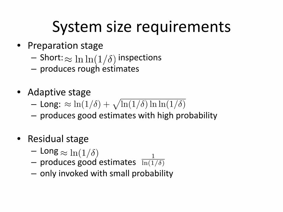
System size requirements• Preparation stage
– Short: inspections– produces rough estimates
• Adaptive stage – Long:– produces good estimates with high probability
• Residual stage– Long – produces good estimates– only invoked with small probability

System size requirements
• Total overhead compared to m*

Conclusions
• Considered resource allocation issues for “learning systems”
• Leads to unusual combination of sequential hypothesis testing with network resource scheduling
• Outlook– Simpler solutions with better performance?– Impact of number of types, and structure of
expertise?