Models of Choice

Agenda

• Administrivia– Readings– Programming– Auditing– Late HW– Saturated– HW 1

• Models of Choice– Thurstonian scaling– Luce choice theory– Restle choice theory

• Quantitative vs. qualitative tests of models.• Rumelhart & Greeno (1971)• Conditioning…• Next assignment

Choice

• The same choice is not always made in the “same” situation.

• Main assumption: Choice alternatives have choice probabilities.

Overview of 3 Models

• Thurstone & Luce– Responses have an associated ‘strength’.– Choice probability results from the

strengths of the choice alternatives.

• Restle– The factors in the probability of a choice

cannot be combined into a simple strength, but must be assessed individually.

Thurstone Scaling

• Assumptions– The strongest of a set of alternatives will

be selected.– All alternatives gives rise to a probabilistic

distribution (discriminal dispersions) of strengths.

Thurstone Scaling

• Let xj denote the discriminal process produced by stimulus j.

• The probability that Object k is preferred to Stimulus j is given by – P(xk > xj) = P(xk - xj > 0)

Thurstone Scaling

• Assume xj & xk are normally distributed with means j & k, variances j & k, and correlation rjk.

• Then the distribution of xk - xj is normal with – mean k - j

– variance j2 + k

2 - 2 rjkjk = jk2

€

P(xk > x j )

= P(xk − x j > 0)

= N(μ k −μ j ,σ jk2 )

0

∞

∫

Thurstone Scaling

€

P(xk > x j )

= P(xk − x j > 0)

= N(μ k −μ j ,σ jk2 )

0

∞

∫

= N(0,1)−zkj

∞

∫ €

zkj =μ k −μ jσ jk

μ k −μ j = zkj ⋅σ jk

Thurstone Scaling

• Special cases:– Case III: r = 0

• If n stimuli, n means, n variances, 2n parameters.

– Case V: r = 0, j2 = k

2

• If n stimuli, n means, n parameters.

Luce’s Choice Theory

• Classical strength theory explains variability in choices by assuming that response strengths oscillate.

• Luce assumed that response strengths are constant, but that there is variability in the process of choosing.– The probability of each response is

proportional to the strength of that response.

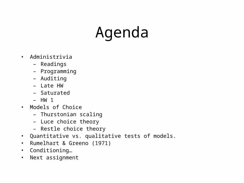
A Problem with Thurstone Scaling

• Works well for 2 alternatives, not more.

Luce’s Choice Theory

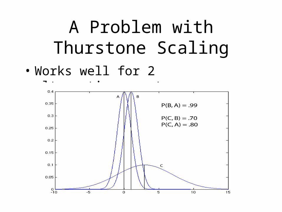
• For Thurstone with 3 or more alternatives, it can be difficult to predict how often B will be selected over A. The probabilities of choice may depend on what other alternatives are available.

• Luce is based on the assumption that the relative frequency of choices of B over C should not change with the mere availability of other choices.

Luce’s Choice Axiom

• Mathematical probability theory cannot extend from one set of alternatives to another. For example, it might be possible for:– T1 = {ice cream, sausages}

• P(ice cream) > P(sausage)

– T2 = {ice cream, sausages, sauerkraut}• P(sausage) > P(ice cream)

• Need a psychological theory.

Luce’s Choice Axiom

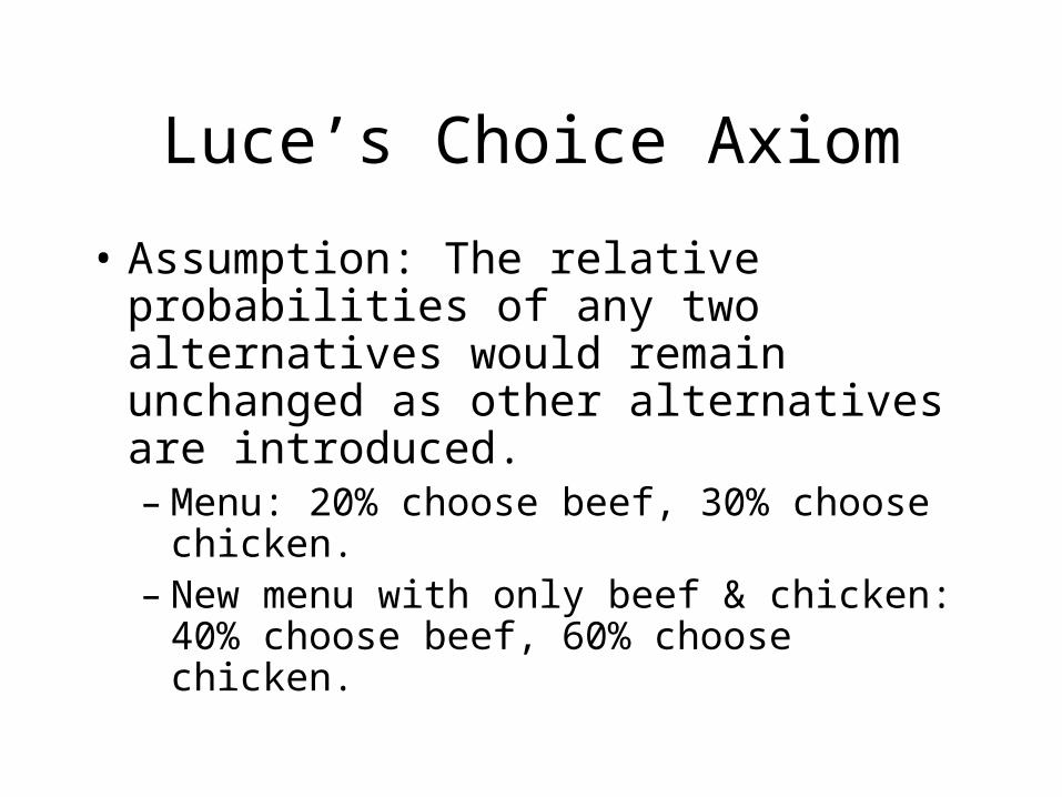
• Assumption: The relative probabilities of any two alternatives would remain unchanged as other alternatives are introduced.– Menu: 20% choose beef, 30% choose

chicken.– New menu with only beef & chicken: 40%

choose beef, 60% choose chicken.

Luce’s Choice Axiom

• PT(S) is the probability of choosing any element of S given a choice from T.– P{chicken, beef, pork, veggies}(chicken, pork)

Luce’s Choice Axiom

• Let T be a finite subset of U such that, for every S T, Ps is defined, Then:– (i) If P(x, y) 0, 1 for all x, y T, then for

R S T, PT(R) = PS(R) PT(S)

– (ii) If P(x, y) = 0 for some x, y in T, then for every S T, PT(S) = PT-{x}(S-{x})

Luce’s Choice Axiom

S

R

T

(i) If P(x, y) 0, 1 for all x, y T, then for R S T, PT(R) = PS(R) PT(S)

Luce’s Choice Axiom•(ii) If P(x, y) = 0 for some x, y in T, then for every S T, PT(S) = PT-{x}(S-{x})

•Why? If x is dominated by any element in T, it is dominated by all elements. Causes division problems.

S

T

X

Luce’s Choice Theorem

• Theorem: There exists a positive real-valued function v on T, which is unique up to multiplication by a positive constant, such that for every S T,

€

PS (x) =v(x)

v(y)y∈S

∑

Luce’s Choice Theorem

• Proof: Define v(x) = kPT(x), for k > 0. Then, by the choice axiom (proof of uniqueness left to reader),

€

PS (x) =PT (x)

PT (S)

=kPT (x)

kPT (x)y∈s

∑

=v(x)

v(y)y∈s

∑

Thurstone & Luce

• Thurstone's Case V model becomes equivalent to the Choice Axiom if its discriminal processes are assumed to be independent double exponential random variables– This is true for 2 and 3 choice situations.– For 2 choice situations, other discriminal

processes will work.

Restle

• A choice between 2 complex and overlapping choices depends not on their common elements, but on their differential elements.– $10 + an apple– $10

XXX X

XXX

P($10+A, $10) = (4 - 3)/(4 - 3 + 3 - 3) = 1

Quantitative vs. Qualitative Tests

Dimensions

Stimulus Legs Eye Head Body

A1 1 1 1 0

A2 1 0 1 0

A3 1 0 1 1

A4 1 1 0 1

A5 0 1 1 1

B1 1 1 0 0

B2 0 1 1 0

B3 0 0 0 1

B4 0 0 0 0

Quantitative vs. Qualitative Tests

Dimensions

Stimulus Legs Eye Head Body

A1 1 1 1 0

A2 1 0 1 0

A3 1 0 1 1

A4 1 1 0 1

A5 0 1 1 1

B1 1 1 0 0

B2 0 1 1 0

B3 0 0 0 1

B4 0 0 0 0

Prototype vs.ExemplarTheories

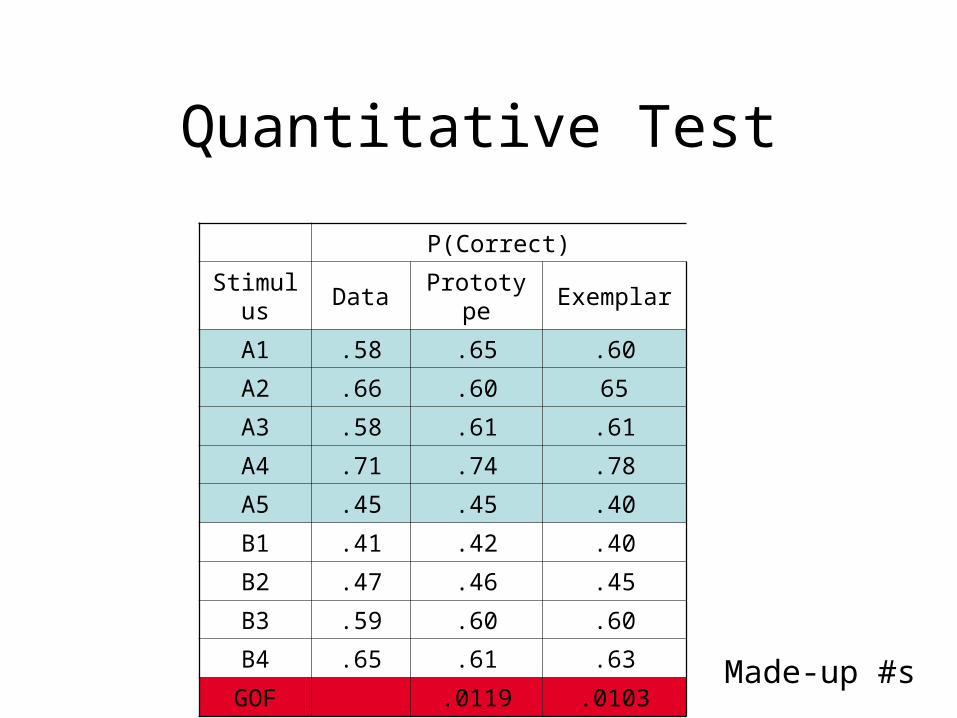
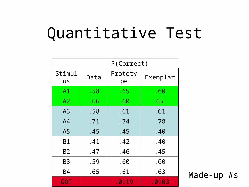
Quantitative Test

P(Correct)

Stimulus Data Prototype Exemplar

A1 .58 .65 .60

A2 .66 .60 65

A3 .58 .61 .61

A4 .71 .74 .78

A5 .45 .45 .40

B1 .41 .42 .40

B2 .47 .46 .45

B3 .59 .60 .60

B4 .65 .61 .63

GOF .0119 .0103 Made-up #s

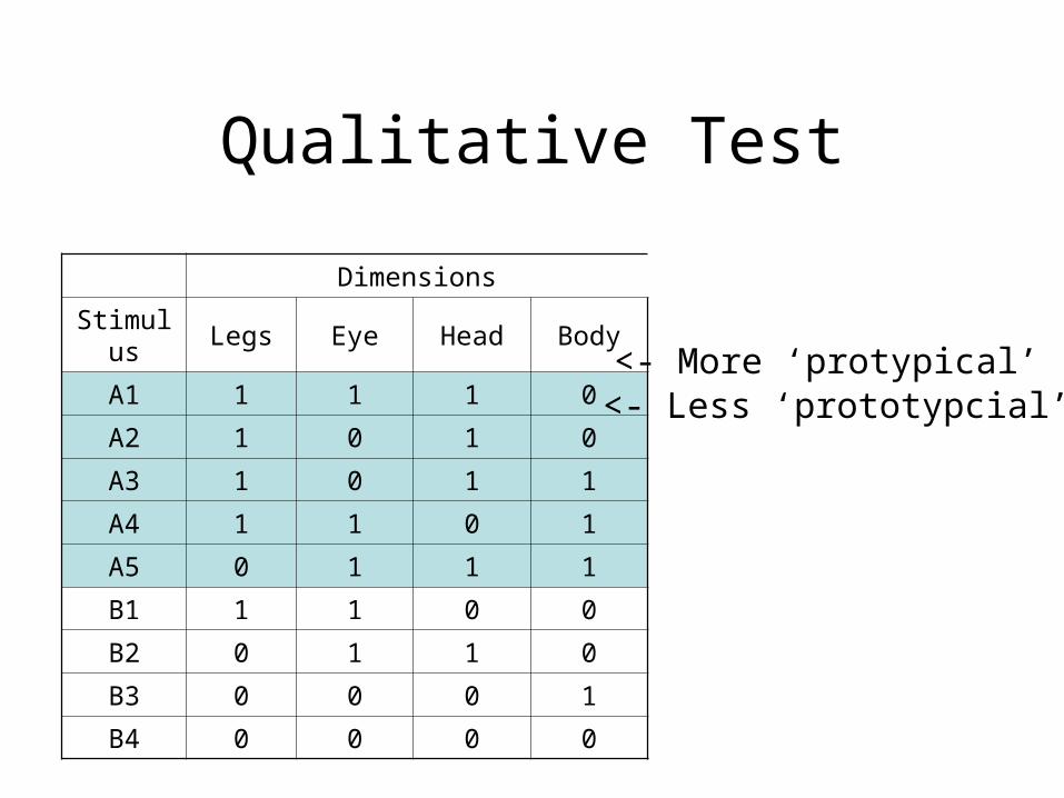
Qualitative Test

Dimensions

Stimulus Legs Eye Head Body

A1 1 1 1 0

A2 1 0 1 0

A3 1 0 1 1

A4 1 1 0 1

A5 0 1 1 1

B1 1 1 0 0

B2 0 1 1 0

B3 0 0 0 1

B4 0 0 0 0

<- More ‘protypical’<- Less ‘prototypcial’

Qualitative Test

Dimensions

Stimulus Legs Eye Head Body

A1 1 1 1 0

A2 1 0 1 0

A3 1 0 1 1

A4 1 1 0 1

A5 0 1 1 1

B1 1 1 0 0

B2 0 1 1 0

B3 0 0 0 1

B4 0 0 0 0

<- Similar to A1, A3<- Similar to A2, B6, B7

Prototype: A1>A2Exemplar: A2>A1

Quantitative Test

P(Correct)

Stimulus Data Prototype Exemplar

A1 .58 .65 .60

A2 .66 .60 65

A3 .58 .61 .61

A4 .71 .74 .78

A5 .45 .45 .40

B1 .41 .42 .40

B2 .47 .46 .45

B3 .59 .60 .60

B4 .65 .61 .63

GOF .0119 .0103 Made-up #s

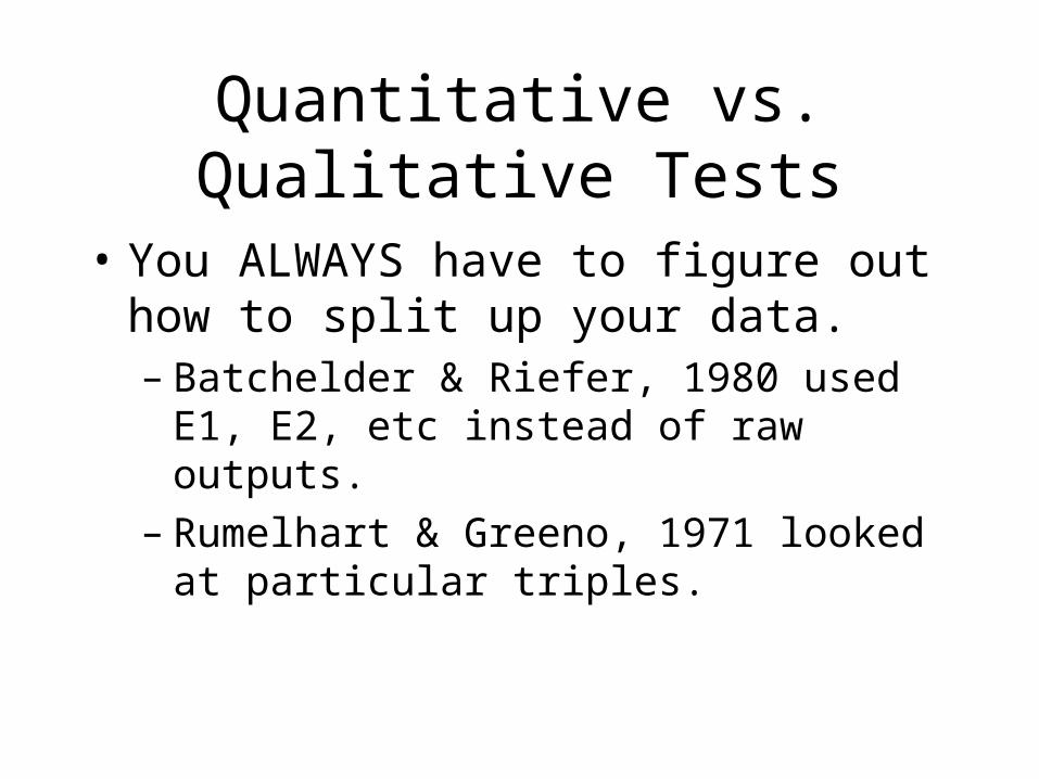
Quantitative vs. Qualitative Tests

• You ALWAYS have to figure out how to split up your data.– Batchelder & Riefer, 1980 used E1, E2, etc

instead of raw outputs.– Rumelhart & Greeno, 1971 looked at

particular triples.

Caveat

• Qualitative tests are much more compelling and, if used properly, telling, but– qualitative tests can be viewed as

specialized quantitative tests, i.e., on a subset of the data.

– “qualitative” tests often rely on quantitative comparisons.