Embed Size (px)
Citation preview
INFRASTRUCTURE
MINING & METALS
NUCLEAR, SECURITY & ENVIRONMENTAL
OIL, GAS & CHEMICALS
Models for Multi-Phase & Single-Phase Flow in Pressure Relieving System Using Bernoulli Integration
About Bechtel Bechtel is among the most respected engineering, project management, and construction companies in the world. We stand apart for our ability to get the job done right—no matter how big, how complex, or how remote. Bechtel operates through four global business units that specialize in infrastructure; mining and metals; nuclear, security and environmental; and oil, gas, and chemicals. Since its founding in 1898, Bechtel has worked on more than 25,000 projects in 160 countries on all seven continents. Today, our 58,000 colleagues team with customers, partners, and suppliers on diverse projects in nearly 40 countries.

GCPS 2015 __________________________________________________________________________
Models for Multi-Phase & Single-Phase Flow in Pressure Relieving System Using Bernoulli Integration
Freeman Self ([email protected]) Sanjay Ganjam ([email protected])
Bechtel Oil, Gas and Chemicals, Inc.
Gerald Jacobs ([email protected]) Virtual Materials Group
Prepared for Presentation at American Institute of Chemical Engineers
2015 Spring Meeting 11th Global Congress on Process Safety
Austin, Texas April 27-29, 2015
Session
DIERS T1G00 Practical Methods for Two-Phase Flow
UNPUBLISHED
AIChE shall not be responsible for statements or opinions contained in papers or printed in its publications

GCPS 2015 __________________________________________________________________________
2
Models for Multi-Phase & Single-Phase Flow in Pressure Relieving System Using Bernoulli Integration
Freeman Self ([email protected]) Sanjay Ganjam ([email protected])
Bechtel Oil, Gas and Chemicals, Inc.
Gerald Jacobs ([email protected]) Virtual Materials Group
Keywords: pressure relief valve, safety valve, orifice, control valve, Bernoulli equation, numerical integration, homogeneous equilibrium
Abstract The Bernoulli (mechanical energy) equation is very important in fluid flow, particularly since it describes how mechanical energy is transformed into other forms of energy. But complications occur in compressible flow since the density changes with pressure. The traditional tool is the analytical solution of the Bernoulli equation. However, to characterize density as a function of pressure for compressible fluid, simplifying assumptions are needed that limit the application. As an alternative, it is becoming more prevalent to use integral methods to numerically solve the Bernoulli equation in compressible flow. This paper will outline the use of numerical integration for several common situations: orifices, relief valves, and control valves. Explanations and derivations will be provided to illustrate how these models can be used for choked / non-choked, single and multi-phase systems.

GCPS 2015 __________________________________________________________________________
3
1. Introduction The Bernoulli (mechanical energy) equation is very important in fluid flow, particularly since it describes how mechanical energy is transformed into other forms of energy. But complications occur in compressible flow since the density changes with pressure. However, to characterize density as a function of pressure for compressible fluid, simplifying assumptions are needed that limit the application. Among them are the assumption of an ideal gas, constant heat capacity and the characterization of density changes with pressure. Despite these limitations, analytical equations are the traditional method but are sometimes used inappropriately. For example, they are used for high-pressure gases which do not exhibit ideal gas behavior. As an alternative, it is becoming more prevalent to use numerical integration to solve the Bernoulli equation in compressible flow. Integral methods are of course not new; the power industry has used them for years for single and two-phase flow of steam and water [Benjamin and Miller-1942]. With increasing computational power, excellent thermodynamic and physical property databases, integral methods may provide good solutions. Furthermore, integral methods lend themselves for use in multi-phases models. 2. General Formulation The general formulation for numerical integration is written as a mass flux [mass/time-area] time the area plus a coefficient.
W [mass/time] = { A0 Kd } { G } G = mass flux [mass/time-area] from either numerical integration or analytical solution A0 = area based at the throat [area] Kd = flow coefficient [dimensionless]
When the mass flux is found by numerical integration it is commonly known as the “direct integration” model. Examples of calculating the integration are provided in several publications [Simpson 1991, Darby 2001, Darby 2002, API-520-I-2014]. For two-phase flow equilibrium (phase, heat and momentum) with the properties described as homogeneous, then the model is additionally called “homogeneous equilibrium model” (HEM). The integration method is thus called “homogeneous direct integration” (HDI). If not at equilibrium, a variety of models have been proposed include “homogeneous non-equilibrium model” and the “frozen equilibrium model”. The integration method may be called “homogeneous non-equilibrium direct integration”, which may be modified to account for fluid slip and phase non-equilibrium provided the appropriate data is available.
2-01

GCPS 2015 __________________________________________________________________________
4
2.1 Mass Flux The mass flux at the vena contracta is evaluated from the integral starting at the initial pressure. Since the flow from the inlet to the vena contracta is essentially frictionless, and the flow distance is short so heat transfer is minimal, the flow may be considered a constant entropy process. The mass flow is then determined from the area at the vena contracta and mass flux. The integral method is especially beneficial since it rigorously evaluates the mass flux for variable densities. Additionally, if the fluid chokes at the vena contracta, the choke pressure and conditions are determined directly. The implementation of the integral method used throughout this study is from the software, VMGSim. [Virtual Materials Group - 2015]. VMG’s APR (Advanced Peng Robinson Equation of State) is used for thermodynamic and physical properties. 2.2 Coefficients The area and flow coefficient, depending on the application, may be calculated separately or combined into a lumped parameter (e.g. control valves). There are two coefficients that are commonly employed. (β2 = A0/A1) The term Cd is generally labelled “coefficient of discharge” or “coefficient of discharge without velocity of approach factor”. When Cd is combined with the “velocity of approach factor”, the term Kd is called the “flow coefficient” or “coefficient of discharge with velocity of approach factor”. Kd is used to simplify the parameter, or used when it is not convenient to calculate beta ratio (e.g. relief valves or control valves). Since the literature uses an inconsistence mix of parameters labelled either C or K, it is important to understand the definition. For example, relief valve vendors call Kd a “discharge coefficient” by truncating the term “with velocity of approach factor”. The coefficient of discharge Cd is used to adjust the theoretical model to match experimental data. The discharge coefficient will differ depending on the model and its assumptions and the quality of the experimental data. Thus discharge coefficients between different models can only be compared qualitatively. It is defined from mass flow W or mass flux G. Cd = Wexperimental / WModel = Gexperimental / GModel
2-03
Kd = Cd / ( 1 – β4 ) 1/2
2-02

GCPS 2015 __________________________________________________________________________
5
3. Flow Orifices (square-edge) 3.1 Overview of Flow Orifices Flow orifices are used for flow measurement and flow restrictions. The application may be complicated due to the variations in configurations, standards, and flow characteristics. This paper will separate the discussion into two main categories: thin orifices and thick orifices. Thin orifices will not choke, while thick orifice will choke depending on the pressure difference. 3.2 Mass Flow Relation (British Standard Units) W [mass/time] = A0 [area] Kd G [mass/time-area] The schematic illustrates the flow streamlines. 3.3 Discharge Coefficients - Thick Orifices – Choking and Non-Choking Flow 3.3.1. Overview of Thick Orifices Thick orifices in gas, flashing liquid, and two-phase flow will choke with sufficient pressure drop. Thus they are also known in the trade as “critical orifices”. Generally for the orifice to choke, the orifice is required to have a certain thickness relative to the orifice hole. Thick orifices, manufactured with square edges, will choke in compressible
3-01
3-02
3-03
Figure 1
Position 1 Position 2 Vena
Contracta
Position 0 Plate
Throat
Fluid streamlines
Position 3 Full
Recovery
W [lb/hr] = A0 [in2] Kd 2407 ρ2 [lb/ft3]
1/2
( 1/ρ) dP P1
P2
∫ P2
where Kd = Cd / ( 1 – β4 ) 1/2 and β2 = (A0 / A1)

GCPS 2015 __________________________________________________________________________
6
flow if the thickness / diameters are approximately greater than 1.0. [Ward-Smith-1979]. Simplistically, choking occurs since the flow remains attached to the lagging edge of the orifice, thus creating a rapid volume expansion at the discharge. The description of flow coefficients in choking flow are complicated since Kds appear to be a function the type of phase during choking (gas or flashing liquid), the number of phases (single or two-phase), the quality (vapor percent) in two-phase flow, equilibrium (phase, thermal or slip), and the plate thickness ratios (thickness / diameter). 3.3.2 Flow Coefficient (Kd) for Choking in Thick Orifices – Data Evaluated Compressible flows in thick orifices under choking conditions were determined by Richardson [Richardson-2006]. The flow coefficient Kd is used since the beta (area ratio) cannot be positively confirmed from the article, although the beta has been roughly estimated as approximately 0.5. The flange-tapped square edge orifices as defined in BS1042. The thickness to diameter ratio was provided only for an 8 mm orifice with a 15 mm plate. There are four basic regimes are discussed. (1) Liquids which are not flashing and not choking. These were not part of the experimental data but have been included for reference, with a nominal Kd of approximately 0.6. (2) Liquid propane, which is flashing and choking at the bubblepoint at it flows through the orifice. This is discussed in Section 3.3.5. (3) Single-phase gas. This includes both natural gas and natural gas+propane, which are single-phase into the orifice. This is discussed in Section 3.3.3. (4) Two-phase gas. This includes only natural gas+propane, which are two-phase into the orifice. This is discussed in Section 3.3.4.
Figure 2 -A
Two-Phase (Natural
Gas+Propane)
Liquid (non-flashing)
Nominal value of Kd
Liquid Propane (flashing)
Note 1
Single Phase (Natural Gas or
Nat Gas+Propane)
Note 1- ΔP/P1 is inlet pressure minus bubblepoint pressure at inlet temperature divided by inlet pressure

GCPS 2015 __________________________________________________________________________
7
3.3.3 Flow Coefficient (Kd) for Choking in Thick Orifices - Single-Phase Natural Gas with Propane Several sets of hydrocarbon data were evaluated. • Natural Gas (100%). The phase inlet to the orifice was gas to the right of the phase
envelope and the flows choked before condensing at the phase envelope. • Natural Gas plus Propane. The phase inlet to the orifice was gas to the right of the
phase envelope. However, small amounts of gas were condensed at the choke point (for all points and less than 8% mass).
For single-phase fluids, the flow coefficient Kd was approximately 0.90. The introduction of propane even with slight condensing had little effect on the discharge coefficient. Both direct numerical integration and Richardson integration gave similar results. These flow coefficients are slightly higher than the air data (Figure 4) for thick orifices. 3.3.4 Flow Coefficient (Kd) for Choking in Thick Orifices - Two-Phase Natural Gas+Propane Natural gas plus propane, in different proportions but approximately 50%-50% were studied for two-phase flow. (Richardson also had a case with condensate added but the results were similar.) The phase inlet to the orifice was two-phase.
Figure 2 -B
Figure 2 -C

GCPS 2015 __________________________________________________________________________
8
Two-phase fluids exhibited slightly higher Kds approximately 0.95. This may be attributed to slip [Giacchette-2014]. When condensate is added to the mixture, the average Kd remains the same although the range increases. Both direct numerical integration and Richardson integration gave similar results. Single phase flow is also shown for comparison; flow coefficients Kd were approximately 0.90. 3.3.5 Flow Coefficient (Kd) for Choking in Thick Orifices - Flashing Propane Liquid Plotted are data for propane which is liquid inlet to the orifice, and which flashes and chokes sharply at the bubble-point. The bubble-points for all points were approximately 90 psia. Propane resembled an incompressible liquid at higher pressures resulting in large mass fluxes and Kds starting at 0.63. At low pressure drops, the propane was slightly more compressible with lower mass fluxes and high Kds. Richardson’s coefficients are approximately 0.6 since Richardson modeled flashing propane as a liquid. However, when using the inlet pressures and choke points calculated from numerical integration, the results followed the same pattern as the plot with variable Kds. (Four points from the data set were not plotted. These had pressures a few pounds above the bubblepoint, choked in the two-phase region, and all had calculated Kds of approximately 2.6.)
Figure 4
Choked at Vena Contracta (Kd nearly constant)
Not-Choked Choked Orifice Exit
β ~ 0
Figure 3
995 psia
126 psia
Bubblepoint ~ 90 psia
1.0
0.9
0.8
0.7
0.6
Kd

GCPS 2015 __________________________________________________________________________
9
3.3.6 Flow Coefficient (Kd) as Function of Plate Thickness for Choking Flow in Thick Orifices using Air The previous data are based on thick orifices with plate thickness /diameter ratio of approximately two (2) and beta of zero. However, it has been found the flow coefficient for thick orifices is constant over a range of plate thickness ratios (thickness / diameter) approximately from 1.0 to 7.0 [Ward-Smith-1979]. For thicker plates, friction is important and the Kds decrease with increasing thickness. 3.4 Discharge Coefficients - Thin Orifices – Not Choking 3.4.1. Overview of Thin Orifices This section has been included to complete the overview of discharge coefficients. When one thinks of flow orifices as measurement devices, it is generally the thin orifices outlined in standards such as ISO-5167, ASME MFC-3M or BS-1042. Unlike thick orifices, the defining characteristic of a thin orifice is that it does not choke. (The standards are limited to low pressure ratios where P2 discharge is 0.8 times P1 inlet or more, although that is sometimes extended to 0.4.) The mass flux always increases with pressure difference; the mass flux does not ever reach a maximum value regardless of the pressure drop. Simplistically, a thin orifice offers little surface for flow attachment and the fluid “jets” through the orifice without forming a deep vena contracta. 3.4.2. Flow Calculations Flow through orifices is calculated with analytical Bernoulli models. The discharge coefficient to be used in the Bernoulli models are given by corresponding fitted equations. The equation coefficient is determined from data for non-choking flow. Standards such as ISO-5167, ASME MFC-3M or BS-1042 provide the equations, which are specific to each type of orifice, and generally provide similar results, although the standards have been frequently modified over the years. In general, limitations include single phase, non-choking, non-pulsating flow, specific location for pressure taps and minimum Reynolds numbers. Refer to each standard for more detailed information.
Engineering handbooks also provide the equations, generally based on one of the above standards. One must be careful since the nomenclature will differ between standards and handbooks. Three correlations are plotted in Figure 6.
Permission to copy is granted under the terms of the GNU Free Documentation License
Figure 5

GCPS 2015 __________________________________________________________________________
10
• Miller-1996 provides a pre-1996 discussion of the standards. The handbook also provides graphs and equations for discharge coefficients. • Crane-2009. Several editions are available but with different formulations and Reynolds number dependencies for discharge coefficients.
3.4.3. Use As a “Loss Coefficient” K Often the pressure drop due to friction in the orifice is required. This may be calculated using the traditional loss coefficient K, which is familiar to engineering applications. Pressure Drop (psi) = K ( ρ v2 / 9278 )
( with density ρ [lb/ft3], velocity v [ft/sec] and includes gc [as 32.2 lb-ft/sec2] )
Many handbooks present variations on the equations to relate K, the loss coefficient, to Cd the discharge coefficient for thin orifices based on pipe velocity. Following are two examples. (β2 = A0/A1) 3.4.4. Coefficient of Discharge To utilize the flow equations and loss coefficient K, the discharge coefficient is needed. Coefficients of discharge are the same for both vapor and liquid. Shown are discharge coefficients Cd calculated from various sources for a beta of 0.5 [Hollinghead-2012, Miller-1996, Crane-2009]. Discharge coefficients used in the standards are calculated
Cd2 β4
( 1 - β4) (1 – β2 ) K ~
[Darby-2001, Eq 10-22]
Cd β2
[ 1 - β4(1 – Cd2)]0.5
K =
-1
[Crane-2009, Eq 4-2]
2
Figure 6
β = 0.5
GCPS 2015 __________________________________________________________________________
11
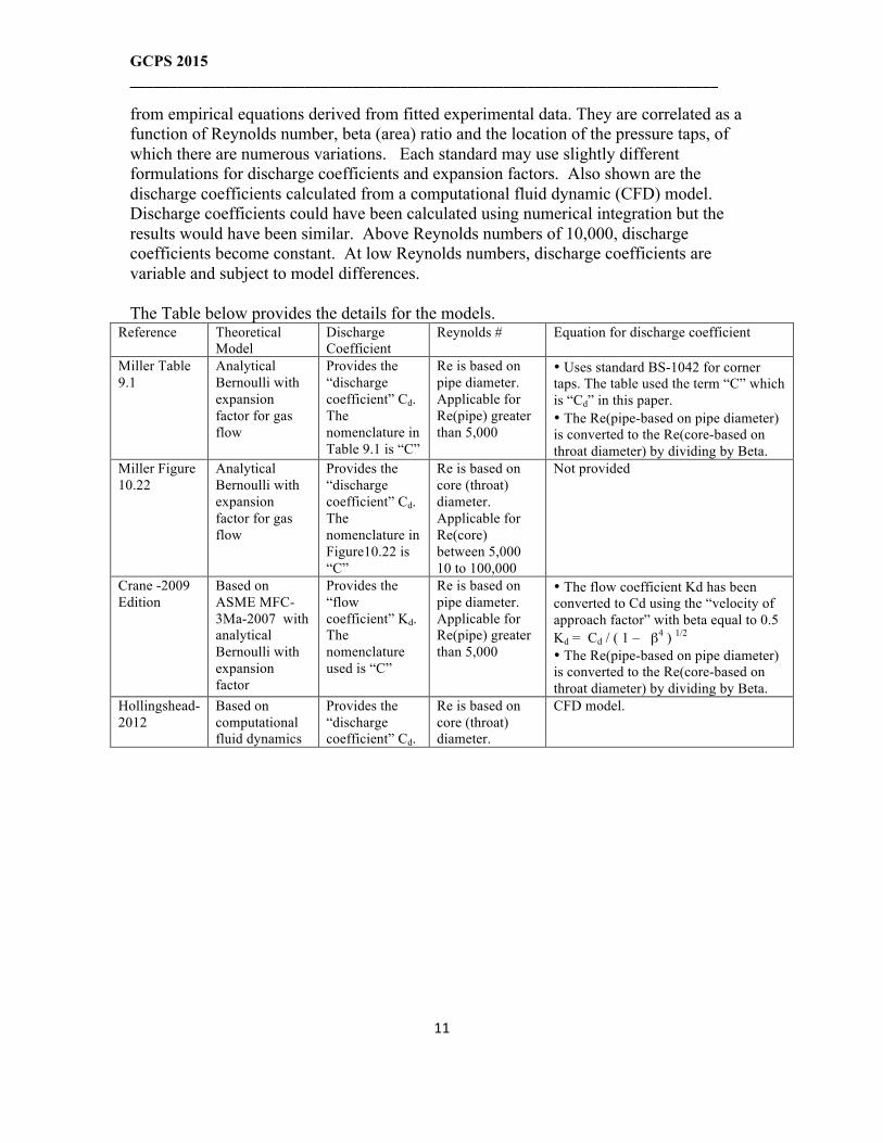
from empirical equations derived from fitted experimental data. They are correlated as a function of Reynolds number, beta (area) ratio and the location of the pressure taps, of which there are numerous variations. Each standard may use slightly different formulations for discharge coefficients and expansion factors. Also shown are the discharge coefficients calculated from a computational fluid dynamic (CFD) model. Discharge coefficients could have been calculated using numerical integration but the results would have been similar. Above Reynolds numbers of 10,000, discharge coefficients become constant. At low Reynolds numbers, discharge coefficients are variable and subject to model differences. The Table below provides the details for the models.
Reference Theoretical Model
Discharge Coefficient
Reynolds # Equation for discharge coefficient
Miller Table 9.1
Analytical Bernoulli with expansion factor for gas flow
Provides the “discharge coefficient” Cd. The nomenclature in Table 9.1 is “C”
Re is based on pipe diameter. Applicable for Re(pipe) greater than 5,000
• Uses standard BS-1042 for corner taps. The table used the term “C” which is “Cd” in this paper. • The Re(pipe-based on pipe diameter) is converted to the Re(core-based on throat diameter) by dividing by Beta.
Miller Figure 10.22
Analytical Bernoulli with expansion factor for gas flow
Provides the “discharge coefficient” Cd. The nomenclature in Figure10.22 is “C”
Re is based on core (throat) diameter. Applicable for Re(core) between 5,000 10 to 100,000
Not provided
Crane -2009 Edition
Based on ASME MFC-3Ma-2007 with analytical Bernoulli with expansion factor
Provides the “flow coefficient” Kd. The nomenclature used is “C”
Re is based on pipe diameter. Applicable for Re(pipe) greater than 5,000
• The flow coefficient Kd has been converted to Cd using the “velocity of approach factor” with beta equal to 0.5 Kd = Cd / ( 1 – β4 ) 1/2 • The Re(pipe-based on pipe diameter) is converted to the Re(core-based on throat diameter) by dividing by Beta.
Hollingshead-2012
Based on computational fluid dynamics
Provides the “discharge coefficient” Cd.
Re is based on core (throat) diameter.
CFD model.

GCPS 2015 __________________________________________________________________________
12
4. Control Valves 4.1 Overview of Control Valve Flow Control valve design exhibits several unusual features. First, the coefficients of discharge for gases and liquids are not dimensionless but have units of measure. As a result, the area and flow coefficient are lumped together as one parameter. Additionally, although control valve equations are generally treated as orifice equations, the flow is calculated based on the service pressure drop (inlet minus discharge pressure) rather than the pressure drop that produces flow, or the difference between the inlet pressure and the vena contracta. This requires accounting for pressure recovery in the valve outlet body. 4.2 Mass Flow Relation The traditional mass flow relationship is utilized. Due to the historical development of control valve sizing, the area and flow coefficient are combined into one parameter, an area-loss coefficient parameter.
W [mass/time] = { A Kd } { G }
The mass flux G is in units of lb/hr-in2, area is in inch2 and pressure in psi. 4.3 Flow Coefficient The area-flow coefficient parameter { A Kd }group is found by equating the ISA control valve equations to traditional orifice equations. For discussion, the original Fisher derivation is easier to physically understand. Refer to Appendix 4 for full derivations including Fisher and ISA-75.01.01. ISA-75.01.01 presents tables for conversion into various units. 4.3.1 Incompressible fluids { A Kd } = { ( FL Cv ) / 38 }, which is a well known relation. The parameter FL is the liquid recovery factor and used to relate the downstream pressure to the vena contracta pressure. Without this conversion, the value of Cv will overstate the flow rate. The liquid discharge coefficient Cv has British Standard units in gallons / minutes -psi1/2.
W [lb/hr] = A Kd 2407 ρT
1/2
( 1/ρ) dP P1
P2
∫ P2
5-01
5-02
5-03

GCPS 2015 __________________________________________________________________________
13
4.3.2 Compressible fluids, • using ISA parameters • { A Kd } = 12.873 [ Cv / Cγ] [(XT Fγ) ½ ] or rearranged • { A Kd } = [ ( Cv / 38)] [ 489.174 (XT Fγ) ½ / Cγ ]
• Fisher parameter Cg
• { A Kd } = [ Cg / 1100 ] or rearranged • { A Kd } = [ Cv * C1 / 1100 ] or rearranged • { A Kd } = [ Cv / 38 ] [ C1 / 28.9 ]
XT is the choking pressure ratio. Fγ is used to adjust heat capacity ratio from air and Cγ is a consolidation of terms that are functions only of the ideal heat capacity ratio. .
4.4. Compressible Ideal Gas - Low Pressure Drop The data is for pressure drops less than 100 psi using air and water. [Buresh & Schuder-1964] In this situation, air is similar to an ideal gas, as judged by the criteria in ISA-75.01.01 Section 7.3, so the ISA equations are applicable. 4.4.1 Adjusting for Pressure at the Vena Contracta – Definition of Gas Pressure Adjustement Coefficient FG The numerical integration model uses the pressure drop that controls the flow (inlet minus vena contracta). On the other hand, the flow rate is experimentally measured based on the service pressure drop (inlet minus discharge), which must be adjusted for use with numerical integration. A “gas pressure-adjustment coefficient” is defined FG and is formulated similar to the “liquid-pressure recovery coefficient” FL (refer to Appendix 4). The parameter FG is called an “adjustment” parameter, since unlike the “liquid-pressure recovery coefficient” FL, the value may be greater than one as well as less than one. A value greater than one large service pressure drops.
• For high-recovery control valves (low C1 and XT), The value of FG is less than one and the choking pressure drop at the vena contracta (P1-Pvc) is greater than the service pressure drop (P1-P2).
5-04 5-05
5-06 5-07 5-08
5-09 FG2 = ( P1 – P2 ) / (P1 – Pvc )
FL (P1 – Pvc )0.5 = ( P1 – P2 )0.5
Figure 7-A
P1 - Pvc P1
Pvc
P2 for high-recovery valves
P1 – P2 “service pressure drop”
P1
P2 for valves with high discharge pressure drops

GCPS 2015 __________________________________________________________________________
14
• For zero-recovery control valves (C1 ~ 29 and XT ~ 0.5), the value of FG is equal to one and the choking pressure drop at the vena contracta is the same value as the service pressure drop (i.e. Pvc = P2). • For large-pressure drop control valves (C1 ~ 35 and XT ~ 0.8), the value of FG is greater than one and the choking pressure drop at the vena contracta (P1-Pvc) is the less than the service pressure drop (P1-P2). This phenomenon is due to large pressure drops at the discharge of the control valve. Double-ported globe valves are examples.
4.4.2 Examples of Converting Pressure Drops To compare, the service pressure drop (used for experimental data and ISA-75.01.01 equations) and flow pressure drop used in numerical integration must be made consistent.
Converting service pressure (such as used in ISA-75.01.01 equation or experimental data) to Flow Pressure Drop, the service pressure drop is adjusted using FG.
(P1-Pvc) = (P1-P2) / FG2 where P1-Pvc is used in numerical integration
Similarly, if numerical integration is used to develop a control valve size, the flow pressure drop from numerical integration is converted to the service pressure drop: (P1-P2) = (P1-Pvc) * FG
2 4.4.3 Value of FG To determine the value of gas pressure-adjustment coefficient FG, the (A KG ) area-flow coefficient parameter is assumed constant. This is a good assumption if the Reynolds number, based on the upstream flow area, is greater than 100,000.
• At choke pressure, the gas area-flow coefficient parameter is:
A * KG-choke = Cg / 1100 = (Cv / 38) * (C1/ 28.9) • At low pressure drops, the gas area-flow coefficient parameter is:
A * KG-low pressure = (Cv / 38) (FG ) • Equating yields an expression for the gas pressure-adjustment coefficient FG. FG, similar to C1 and XT, indicates the degree of pressure recovery.
FG = C1 / 28.9 (Fisher parameters) or FG = ( 490 / Cγ) ( Fγ XT )0.5 = ( 1.38 / C2) ( Fγ XT )0.5
Figure 7-B
A * KG-choke = Cg / 1100 A * KG-choke = (Cv / 38) * (C1/ 28.9)
A * KG-low pressure = (Cv / 38) (FG )
Pressure Drop
Flow
Choke
Area-flow coefficient parameter is constant when: A * KG = (Cg / 1100) = (Cv / 38) (FG ) and FG = (C1/ 28.9)

GCPS 2015 __________________________________________________________________________
15
Since ( Cγ / C2) = 355.9 for all values of γ. (ISA-75-01.01)
4.4.4 Comparison of Fisher Air Data Figures 8 through 10 present six control valves with flow data (labelled “Fisher”) compared with ISA-75.01.01 (labelled “ISA) predictions and numerical direct integration (labelled HDI). The data matches quite well for all six control valves. The control valves include both high-recovery and low recovery valves. The pressure drop is (P1 – Pcv). 4.4.5 Choke Pressures The choke pressures from the data and ISA predictions are different from numerical integration. The integration choke points are calculated directly from the integral using densities. The ISA-75.01.01 choked points are “pseudo” choke pressures determined by the equation so that the expansion factor Y ix equal to 0.667 and are not expected to exactly match the actual choke point. The data choke points are taken from the graph in the article where the flow rate is a maximum, and are not expected to be accurately read especially since many plots are log scale. 4.5 Non-Ideal Gas The ISA-75.01.01 gas equations were developed from the ideal gas Bernoulli equation. The ISA criterion states the equations are valid when the specific heat ratio ranges between 1.08 and 1.65. For Figure 8
Figure 10

GCPS 2015 __________________________________________________________________________
16
specific heat ratios above 1.65, numerical integration should provide reasonable accuracy, since the mass flux is determined using actual densities and thus is appropriate for high-pressure gases. In contrast, Marc Riveland [Riveland-2012 and Riveland-2014] has explored non-ideal gas flow using the ISA concept. He has proposed a non-linear modification to the factor Fγ to account for non-ideal gas behavior so that the ISA-75.01.01 equations may be used directly. His modification agrees well with an analytical model that uses the isentropic exponent ratio rather than the specific heat ratio. 4.6 Incompressible Liquid As expected, numerical integration matches the ISA-75.01.01 equations well. 4.7 Flashing Liquid Completely incompressible liquids do not choke since the velocity of a sound wave in the liquid is higher than the velocity of the liquid flow. However, if a liquid containing gas flashes, then the mixture density decreases, such that choking may occur. This phenomenon is often called off-gassing or out-gassing. An example in amine system is the flashing of the rich amine from the bottom of the absorber through the liquid level control valve. The calculation of the pressure at which the flows choke, due to flashing gas, is important for the control valve sizing. The traditional method Figure 9
GCPS 2015 __________________________________________________________________________
17
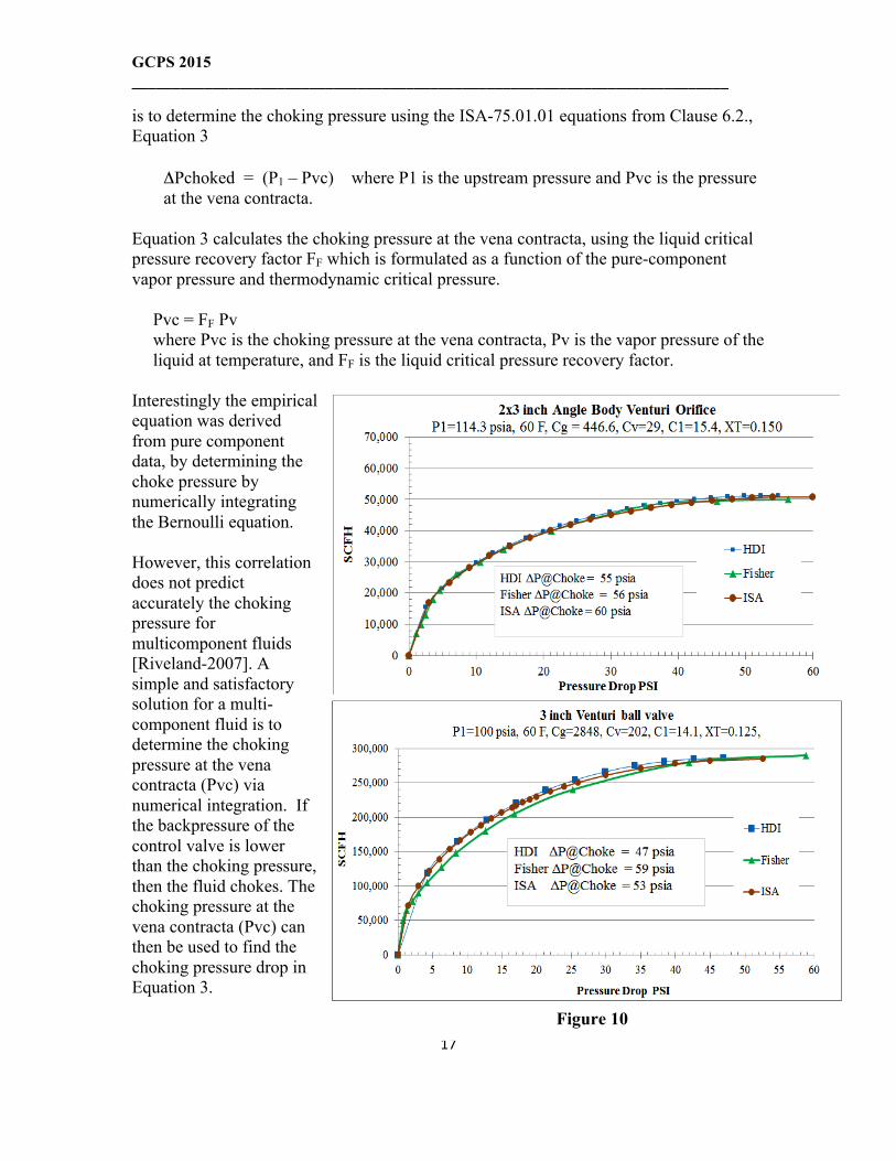
is to determine the choking pressure using the ISA-75.01.01 equations from Clause 6.2., Equation 3
ΔPchoked = (P1 – Pvc) where P1 is the upstream pressure and Pvc is the pressure at the vena contracta.
Equation 3 calculates the choking pressure at the vena contracta, using the liquid critical pressure recovery factor FF which is formulated as a function of the pure-component vapor pressure and thermodynamic critical pressure.
Pvc = FF Pv where Pvc is the choking pressure at the vena contracta, Pv is the vapor pressure of the liquid at temperature, and FF is the liquid critical pressure recovery factor.
Interestingly the empirical equation was derived from pure component data, by determining the choke pressure by numerically integrating the Bernoulli equation. However, this correlation does not predict accurately the choking pressure for multicomponent fluids [Riveland-2007]. A simple and satisfactory solution for a multi-component fluid is to determine the choking pressure at the vena contracta (Pvc) via numerical integration. If the backpressure of the control valve is lower than the choking pressure, then the fluid chokes. The choking pressure at the vena contracta (Pvc) can then be used to find the choking pressure drop in Equation 3.
5-03
Figure 10

GCPS 2015 __________________________________________________________________________
18
4.8 Two-Phase Flow Two-phase flow is not covered by IS-75.01.01. However, numerical integration provides a platform for predicting two-phase flow. But, there are several issues to address. • A common description of mixed density is 1/ρT = x/ρG + (1-x)/ρL where x is the vapor mass fraction and ρT, ρG, amd ρL are the densities for mixed, gas and liquid respectively • Equilibrium and non-equilibrium may be incorporated into numerical integration, provided non-equilibrium data is available • A flow coefficient relationship is needed. Based on typical values for a variety of control valves, the flow coefficient for gas (Kd-G) and the flow coefficient for liquids (Kd-L) may be obtained from parameters in Table D-2, ISA-75.01.01. High-recovery valves such as venturi valves have ratios approaching 1.0. Low-recovery valves have high ratios. Refer to Figure 11. • Liquids: { A * Kd-L } = (Cv / 38) (FL ) • Gases: { A * Kd-G } = [ Cv / 38 ] [ C1 / 28.9 ] • Then the ratio ( Kd-G / Kd-L ) = C1 / (28.9 FL)
4.9 Multi-Stage Control Valves Multi-stage control valves have trims with several stages separated by a gap. The trim may have single or multiple flow passages. The valves are used to create large pressure drops and to reduce noise by lowering the velocities in the valve. Since friction is high, flow coefficients need to be reformulated with a friction component. ISA-75.01.01 (Annex B) provides a method for compressible flow through multistage control valves consistent with the equations for single-stage valves. These valves will not be considered at this time.
Figure 11
high-recovery
low-recovery

GCPS 2015 __________________________________________________________________________
19
5. Pressure Relief Valves 5.1 Overview of Relief Valve Flow The use of numerical integration has been most often applied to relief valves, rather than orifices and control valves. The integral method has proven successful for relief valves under a full range of fluids and conditions, including flashing liquids, high-pressure gases, dense-phase fluids and multi-phase fluids for both choking and non-choking conditions. Additionally the equation may be easily arranged to account for fluid slip between gas and liquid phases (i.e. the velocity of the phases are not equal) and phase non-equilibrium if appropriate data are available. 5.2 Mass Flow Relation The mass flow relation will be written in terms of mass flux G [mass/time-area] and area A. 5.3 Discharge Coefficient The discharge coefficients for industrial relief valves may be obtained either from the National Board Pressure Relief Device Certifications NB-18 (“Redbook”), or API Standard 526 “Flanged Steel Pressure Relief Valves”, which provides a standard framework for valve physical size and discharge coefficients. Relief valve vendors have configured their designs such that either NB-18 or API-526 discharge coefficients and areas can be utilized. To meet the requirements of ASME Boiler & Pressure Vessel Code, the parameters have been selected such that the following relationship is applicable. As such, it should be emphasized that parameters from NB-18 should not be comingled with parameters from API-526.
{ Kd * Area }-based on NB-18 < { Kd * Area }-based on API-526 API-526 was developed to facilitate engineering projects and it is commonly used since the parameters are almost all standard regardless of the vendor.
• For gases, Kd is 0.975 for many major vendors based on API Standard 526 “Flanged Steel Pressure Relief Valves”. • For liquids, Kd varies between vendors but is on the order of 0.75 based on API-526 values. • For multi-phase flow, there are several methods to obtain the mixed discharge coefficient. • Average the liquid and gas Kds based on the volume-weighted average of the gas and liquid flows
4-01 W [lb/hr] = A0 Kd 2407 ρT
1/2
( 1/ρ) dP P1
P2
∫ P2

GCPS 2015 __________________________________________________________________________
20
• Average with the volume-weighted flows, where each phase is calculated with the respective Kd • Kds are chosen depending on whether the flow chokes
5.4. Incompressible Fluids Numerical integration and analytical equations provide similar relief sizing results for constant density fluids. For fluids that may be have variable densities, such as those above the peak of a phase envelope (typically called critical or dense-phase fluids), numerical methods will provide more accurate representation of the mass flux than an incompressible analytical method. 5.5. Compressible Gas - Ideal and Non-Ideal Gas API Standard 520-Part I, section 5.6.1 suggests a criterion when it is appropriate to assume that the gas is ideal and relief valve sizing results are acceptable. • If the real compressibility factor Z is between 0.8 and 1.1 (generally low pressures and high temperatures), then ideal gas behavior may be assumed. • If the real compressibility factor Z is less than 0.8 or greater than 1.1, then the behavior may not be ideal and the use of analytical equations may not be appropriate. In this case, numerical integration may be used.
5.6. Two-Phase Flow Two-phase flow in relief valves provided the interest
Figure 12

GCPS 2015 __________________________________________________________________________
21
for development of methods other than ideal-gas or incompressible liquids. The subject is well covered in the literature, and the intent is to provide only a short summary. Although there are have been many models proposed, there are two primary methods covered by international standards. • API Standard 520-Part I (2014) discusses numerical integration and the Omega method, which is an analytical development for two-phase flow. Other references for the Omega methods include [Leung-2004, Diener-2004]. Since the Omega method is analytical method, it will not be considered in this paper. • ISO-4126-Part 10 (2010) discusses only the Omega method.
The summary of the numerical integration method is based on several articles by Ron Darby [Darby-2004, Darby-2005]. The references for the experimentally measured data are provided in the articles. The two examples show that numerical integration provides an adequate model of two-phase flow. The air-water data may be modeled assuming equilbrium. However, the data for team and water shows that a non-equilibrium model provides a better fit. The discharge coefficients are chosen depending on whether the flow chokes. [CCPS-1998]. This method accommodates compressible gas, multi-phase flow or choking liquids.
• If the flow chokes, only the inlet nozzle flow of the relief valves is involved and “gas” discharge coefficient is used • If the flow does not choke, both the inlet nozzle and body downstream of the vena contracta is involved and the “liquid” discharge coefficient is used.

GCPS 2015 __________________________________________________________________________
22
7. Conclusions We demonstrate the use of numerical integration for flow through orifice, control valves and relief valves. Numerical integration is a simple to apply, easily checked, and accurate method that is may be extended to non-ideal gases and multi-phase flow with and with-out equilibrium conditions. ● Orifices. Single-phase hydrocarbon flows through choking thick orifices exhibit flow coefficients Kd expected for gases. On the other hand, two-phase flow into the orifice of natural gas plus propane exhibited slightly higher flow coefficients, possibly due to non-equilibrium effects of the propane and methane. The experimental data for liquid propane, which chokes at the propane bubble point, displays variable flow coefficients, depending on the choking pressure drop. At high pressure drops, the flow coefficient is similar to a liquid; at low pressure drops, the flow coefficients resemble gas flow. ● Control Valves. Numerical integration is an elegant and accurate method to predict ideal gas flows. Since the mass flux is calculated from actual densities, numerical integration is also appropriate for non-ideal gases. Additionally, the method offers a conceptual basis for two-phase flow. ● Relief Valves. Numerical integration has proven successful for relief valves under a full range of fluids and conditions, including flashing liquids, high-pressure gases, dense-phase fluids and multi-phase fluids for both choking and non-choking conditions. Additionally the equation may be easily arranged to account for non-equilibrium conditions if appropriate data are available. 8. Nomenclature A area [length2] { A Kd } area-flow coefficient parameter for control valves C “discharge coefficient” used by some publications; same as Cd Cγ consolidation of terms that are functions only of the ideal heat capacity ratio k CC = A2 / A0 contraction coefficient = (A2/A1) / β2 since (A0 / A1) = β2. Cc2 = 1/α2 when velocity profile at position 2 is defined as α2 = (A0/A2)2 Cd “discharge coefficient” or “discharge coefficient without velocity of approach factor” (W experimental / W model) Cv flow coefficient for control valve [volume/time-pressure^0.5] Cg apparent gas discharge coefficient for choked gas flow C1 parameter representing pressure drop, defined by Cg = C1 Cv C2 consolidation of terms that are functions only of the heat capacity ratio and used to adjust data taken on air for different values of k. DH hydraulic diameter FL liquid pressure-recovery coefficient for control valves FG gas pressure-adjustment coefficient for control valves

GCPS 2015 __________________________________________________________________________
23
Fγ adjustment for ideal gas heat capacity ratio = γ / 1.4 ƒ Fanning friction factor gc constant for British Standard Units 32.174 ft-lb/sec2 K “loss coefficient” or “resistance coefficient” or “K factor” or “pressure loss coefficient” or “friction loss factor”, depending on publication Kd “flow coefficient” or “discharge coefficient with velocity of approach factor”, or “meter coefficient’ or “discharge coefficient” for relief valves, depending on publication L length of pipe M molecular weight P pressure [(mass*length / time2 ) / length2 ] or [mass / time2 – length] R the gas constant T temperature v velocity [length/time] W mass flow rate [mass/time] x vapor mass fraction XT critical pressure ratio for gas at choking Y “expansion factor” which accounts for density changes for a gas Z compressibility factor α velocity profile adjustment β area ratio ( A0/A1 )0.5
ρ density [mass/volume] γ ideal gas heat capacity ratio Subscripts 0 throat position 1 upstream position 2 vena contracta position 3 vena contracta position 3 downstream position T mixed phase G gas density L liquid density γ pertains to heat capacity ratio

GCPS 2015 __________________________________________________________________________
24
9. References 9.1 Articles • M.W. Benjamin and J.G. Miller, “The flow of a Flashing Mixture of Water and Steam Through Pipes”, Transactions of the American Society of Mechanical Engineers, Volume 64, October 1942 • J. F. Buresh and C.B. Schuder, “Development of a Universal Gas Sizing Equation for Control Valves”, ISA Transactions, Vol 3, 1964, pp 322-328 • R. Darby, Chemical Engineering Fluid Mechanics, 2nd Ed, CRC Press, 20001. • R. Darby, “On Two-Phase Frozen & Flashing Flows In Safety Relief Valves”, JLPPI, Vol 17, 2004, pp 255-259 • R. Darby, F. Self, and V. Edwards, “Properly Size Pressure Relief Valves For Two Phase Flow”, Chemical Engineering Magazine, June 2002, pp 68-74 • R. Darby, F. Self, and V. Edwards, “Methodology For Sizing Relief Devices For Two Phase (Liquid/Gas) Flow”, AIChE Spring National Meeting, Session T5a12 - Pressure Relief Systems, April 23-27, 2001 • R. Diener, and J. Schmidt, “Sizing of Throttling Device for Gas/Liquid Two-Phase Flow, Part 1: Safety Valves, Process Safety Progress, Vol 23(4), March 2004, pp335-344, • G. Giacchette, M. Leporini, B. Marchetti, and A. Terenzi, “Numerical Study of Choked Two-Phase Flow of Hydrocarbons Fluids Through Orifices”, Journal of Loss Prevention in the Process Industries, Vol 27 (2014), pp 13-20 • C. L. Hollingshead, “Discharge Coefficient Performance of Venturi, Standard Concentric Orifice Plate, V-Cone, and Wedge Flow Meters at Small Reynolds Numbers”, Graduate Thesis Paper 869, Utah State University, May 2011 <http://digitalcommons.usu.edu/etd/869> • J. C. Leung, J.C., “A theory on the discharge coefficient for safety relief valve”, JLPPI, Vol 17, 2004, pp 301-313 • S. M. Richardson, G. Saville, S. A. Fisher, A. J. Meredith and M. J. Dix, “Experimental Determination Of Two-Phase Flow Rates Of Hydrocarbons Through Restrictions”, Trans IChemE, Part B, Process Safety and Environmental Protection, 2006, Volume 84(B1) January 2006, pp 40–53 • M. Riveland, “Use of Control Valve Sizing Equations with Simulation Based Process Data”, Presented at ISA Automation Week 2012. • M. Riveland, “The Impact of non-Ideal Compressible Fluid Behavior on Process Control Valve Sizing and Selection”, Presented at Valve World Conference 2014. • M. Riveland and V. Mezzano, “Critical Service Control Valve Sizing and Selection for Hydrotreating”, presented at Emerson Global Users Exchange, 2007 • L. L. Simpson, “Estimate Two-Phase Flow in Safety Devices”, Chemical Engineering Magazine, August 1991, pp 98-102. • A.J. Ward-Smith, “Critical Flowmetering: The Characteristics of Cylindrical Nozzles with Sharp Upstream Edges”, International Journal Heat and Fluid Flow, Vol 1(3), September 1979, pp 123-132 • Virtual Materials Group, Inc. VMGSim Process Simulator, Version 9.0, Virtual Materials Group, Inc., Calgary, Alberta, Canada, 2015

GCPS 2015 __________________________________________________________________________
25
9.2 Books • CCPS. Guidelines for Pressure Relief and Effluent Handling Systems, Center for Chemical Process Safety (CCPS), American Institute of Chemical Engineers, New York, March 1998 • Crane, “Flow of Fluids” TP-410, 2009 Edition, 2013 • Richard W. Miller, Flow Measurement Engineering Handbook, 3rd Edition, McGraw-Hill, 1996 • National Board of Boiler Inspectors, Pressure Relief Device Certifications, (Http:/www.nationalboard.org/Redbook/Redbook.html) 9.3 Standards • API Standard 520-I (9th Edition, July 2014), “Sizing, Selection, and Installation of Pressure-Relieving Devices-Part I-Sizing & Selection”, Section 5.10 and Annex C, • API Standard 526 (6th Edition, July 2009), “Flanged Steel Pressure Relief Valves” • ASME MFC-3M-2004 “Measurement of Fluid flow in Pipes Using Orifices, Nozzles and Venturi”. • BS-1042-1-1.2-1989 “Measurement of fluid flow in closed conduits.” • IEC-60534-2-3 (2nd Edition march 2007), “Industrial-process control valves – Part 2-3: Flow capacity – Test procedures” • IEC-60534-2-1 (2nd Edition march 2011), “Industrial-process control valves – Part 2-1: Flow capacity – Sizing equations for fluid flow under installed conditions” • ISA-75.01.01 (1st Edition August 2012) (60534-2-1 MOD), “Industrial-Process Control Valves - Part 2-1: Flow capacity – Sizing equations for fluid flow under installed conditions” • ISO-4126.10.01 (1st Edition-Oct 2010), “Safety devices for protection against excessive pressure - Part 10: Sizing of safety valves for gas/liquid two-phase flow” • ISO 5167-2:2003 “Measurement of fluid flow by means of pressure differential devices inserted in circular cross-section conduits running full - Part 2: Orifice Plates, 2003

GCPS 2015 __________________________________________________________________________
26
Appendix 1 – Bernoulli Equation – General Form - Details of Derivations The mechanical energy steady-state balance illustrates how energy is transformed due to kinetic energy, potential energy, process work (free energy), mechanical work and friction loss. The balance is shown as flowing from Point 1 to Point 2; the signs of the terms reflect this convention. Please note that sign convention differs between authors so careful attention should be exercised. The terms are shown as energy per mass {[(length/time)2-mass] / mass}. The mechanical energy steady-state balance will account for errors due to the velocity profiles, friction estimates, and others, by introduction of three adjustable parameters.
• α are used to adjust for velocity profiles. For example, in turbulent flow with a flat velocity profile α = 1. • Cd is the “discharge coefficient”, or actually correlating parameter which accounts for deviations in assumptions. The discharge coefficient is used to calibrate the equation to flow data and is the ratio of the experimentally measured flowrate (or mass flux) to that calculated from the model. Thus the discharge coefficient will differ depending on the model and assumptions and the quality of the experimental data. Discharge coefficients between different models can only be compared qualitatively. Finally, the placement of the discharge coefficient within the equation is based on convenience and is not theoretically established.
Expanding above equation and adding the parameters, the following general equation is the starting point for the individual situations.
A1-01
A1-02
( 1/ρ) dP
P1
P2
∫ g (h1 – h2) + + - ∑ ( ½ v2 ƒ 4L/DH ) ∑ ( ½ v2 K ) - = 0 ½ v12
α1 α2 ½ v2
2 - Cd2
( 1/ρ) dP
P1
P2 ∫ Δ ½ v2 g Δ h W
s + + + -- ∑ ( ½ v2 ƒ 4L/DH ) ∑ ( ½ v2 K ) -- = 0
Kinetic energy –work to change the velocity of the fluid
Process work due to pressure changes
Friction loss or the irreversible conversion of friction into thermal energy for turbulent flow in straight pipe
Friction loss or the irreversible conversion of friction into thermal energy
Potential energy due to elevation
Work done by fluid to surrounding system (e.g. shaft of a machine)

GCPS 2015 __________________________________________________________________________
27
Appendix 2 – Flow Orifices (square-edge) - Details of Derivations 1. The general equation will now be modified to develop the basic equations for numerical integration. The order of the integral and signs must be carefully considered since different authors integrate in different orders. The relief valve is physically short in length so that wall friction as a function of straight pipe length is neglected. However other sources of friction are included. In this paper, the friction formulation K will be related to the inlet velocity. The K will take a different form if related to discharge velocity. If comparing to other forms in the literature, some authors assume the kinetic energy adjustment for the shape of the velocity profiles (alpha) is a multiplier, rather than a divisor. 2. The equation will be written at the vena contracta (position 2) since that is the position where choking occurs. Note the change in the signs.
3. The Bernoulli equation explains how energy is transformed. And together with the continuity equation, it can establish the mass flow. The kinetic energy term will be used since it contains the velocity term. 4. The mass flow is the same regardless W = W1 = W2 = W0
W = ρ1 v1 A1 = ρ2 v2 A2 or v1
2 = v2
2 [ρ2 A2 / ρ1 A1]2
v22 = W2 / [ ρ2
2 A22 ]
+ ∑ ( ½ v12 K ) + = ½ v1
2 α1 α2
½ v22 -- ( 1/ρ)
dP
P1
P2 ∫ Cd
2
(e.g. ( ½ v2 α ) rather than ( ½ v2 / α ) A2-01
A2-02
A2-03
A2-04
Figure 1
Position 1 Position 2 Vena
Contracta
Position 0 Plate
Throat
Fluid streamlines
Position 3 Full
Recovery
0 0
g (h1 – h2) + + - ∑ ( ½ v2 ƒ 4L/DH ) ∑ ( ½ v2 K ) - = 0 ½ v12
α1 α2 ½ v2
2 - Cd2 ( 1/ρ) dP
P1
P2 ∫

GCPS 2015 __________________________________________________________________________
28
5. We can rearrange into a typical form by rearranging terms and taking square root. The following is a common form of the equation. 6. The general equation can be made more specific for orifices or venturis.
• As usual, a Beta ratio is defined using A1 and A0 as (A0 / A1) = β2. • Since the throat is a known experimental parameter, it is convenient to write the equations for the throat (position 0). Thus we need to define a relationship between A0 and A2. Typically, a contraction coefficient is defined as follows. The relationship to the velocity profile is discussed later. A2 = A0 CC or CC = A2 / A0
• For venturi meters, A2 ~ A0 and CC ~ 1 • For orifices, the vena contracta (A2) is narrower than the orifice throat (A0). We can then combine the ratio of (A2/A1) as: (A2/A1) = β2CC. This will be substituted in the above. • Consolidate terms in the dominator and considering signs
7. One last expression will complete the general equation, which still includes a friction term. This form includes the Beta ratio in the denominator.
• At the discharge, the velocity profile for the orifice may be given by α2 = (A0/A2)2. This is an important assumption since it provides a method to quantify alpha α. Further, by assuming a profile for α2, then α2 may be eliminated and we only need a value for α1. As noted earlier for venture meters, A0 ~ A2 and the velocity profile results in α2 = 1.0. • Note that since the contraction coefficient is defined as Cc = A2 / A0
• With the above, then we can write an identity is Cc2 = 1/α2.
A2-05
A2-06 W =
( α2 )0.5 ρ2 A2 Cd
1/2
2 ( 1/ρ) dP
P1
P2 ∫
{ 1 – ( [Cc β2 (ρ2 /ρ1)]2 [ (α2 /α1 ) – (α2 K) ] ) } 1/2
W =
( α2 )0.5
{ 1 - ( [ α2 /α1 ][ ρ2 A2 / ρ1 A1] 2 )
+ ∑ ( [ K α2 ] [ ρ2 A2 / ρ1 A1] 2 ) } 1/2
ρ2 A2 Cd
1/2
2 ( 1/ρ) dP
P1
P2 ∫

GCPS 2015 __________________________________________________________________________
29
9. The value of α1 = 1.0, since the flow is turbulent at the inlet. If we assume that friction is considered sufficiently small to be included in the coefficient of discharge, then K ~ 0. Also β2 = (A0 / A1)
10. The discharge coefficient term may be rearranged depending on whether the fluid is a vapor or liquid or two-phase.
If the differences in densities between the inlet and discharge are sufficiently small, the error is included in the coefficient of discharge. In this form, the term discharge coefficient Cd is sometimes called “coefficient of discharge without velocity of approach factor”. [Crane-2009, Miller-1996] Similarly, the flow coefficient Kd is called the “coefficient of discharge with velocity of approach factor”.
A2-08
A2-09
A2-07
Kd = Cd / ( 1 – β4 ) 1/2
A2-10 Kd = Cd / (1 – [ β4 (ρ2 /ρ1) 2 ] ) 1/2
A2-11
W = ρ2 A0 Cd
1/2
2 ( 1/ρ) dP
P1
P2 ∫
{ 1 – ( [ β2 (ρ2 /ρ1) ]2 [ (1 /α1 ) – ( K) ] ) } 1/2
W =
ρ2 A0 Cd
1/2
2 ( 1/ρ) dP
P1
P2 ∫
{ 1 – [ β4 (ρ2 /ρ1) 2 ] } 1/2
W G = = ρ2
1/2
2 ( 1/ρ) dP
P1
P2 ∫
{ 1 – [β4 (ρ2 /ρ1)]2 ] } 1/2
A0 Cd

GCPS 2015 __________________________________________________________________________
30
Appendix 3 – Control Valves - Details of Derivations An expression for the term representing area and discharge coefficient is needed in terms of parameters utilized by the control valve industry. App 3.1 Area and Flow Coefficient For Choking Gas An expression for the area-gas discharge coefficient parameter for choking will be found by equating the analytical Bernoulli equation to the choking control valve gas equation.
• Bernoulli Equation for Choking Gas Flow. W = A * KGAS * Cγ * P1 * (M/TZ) ½
Where: • KGAS is the gas flow coefficient • Cγ is a consolidation of terms that are functions only of the heat capacity ratio γ=Cp/Cv. (For ideal gas, γ=Cp/ [Cp – R] where R is the gas constant ) • Cγ = 520 * [ γ * { [2/(γ+1)] ((γ+1)/(
γ-1)) } ] 0.5 (e.g. Cγ is 355.9 for air.)
• Fisher Equation for Gas Flow. The historical Fisher equation will be used since it is the traditional form. The equivalent ISA-75.01.01 is provided in a later section. From air data Fisher has defined the apparent gas discharge coefficient for choked gas flow as Cg, which is determined experimentally. Q = Cg C2 P1 [520 / (T SG)] ½ (refer to Buresh & Schuder eq 13) W = 0.3234 * Cg * C2 * P1 * (M/TZ) ½
Where: • SG is defined as M / 28.965 with the molecular weight of air being 28.965 • Q [scf/h] = W [lb/hr] * 379.49 [scf/mole] / M [lb/mol] at 14.696 psia & 60°F. • C2 = [ 2.0665 ] * [ { γ/(γ+1) } * { [2/(γ+1)] (2 / (
γ-1) } ] 0.5 where C2 is a
consolidation of terms that are functions only of the heat capacity ratio and used to adjust data taken on air for different values of k. (e.g. C2 is 1.00 for air)
• Area and Discharge Coefficient for Choking Gas Flow {A KGAS } – Fisher Formulation. When equated both equations { A KGAS } = Cg / 1100 = (Cv /38)(C1/28.95) Where:
• KGAS is the gas flow coefficient • ( Cγ / C2) = 355.9 for all values of γ. • C1 = Cg/Cv or Cg = C1*Cv by definition
A3-01
A3-02
A3-03

GCPS 2015 __________________________________________________________________________
31
App 3.2 Area and Flow Coefficient For Incompressible Liquid The expression for incompressible flow is found by equating Bernoulli equation with ISA-75.01.01 expression.
• Bernoulli equation. Analytical Bernoulli equivalent in terms of area and liquid discharge coefficient Q GPM = A * KLIQUID 38 ((P1 - PVC ) / G ) 0.5
where P1 is the upstream pressure and PVC is the pressure at the vena contracta. • ISA-75.01.01 Expression. For the liquid discharge coefficient Cv is defined. Q GPM = Cv ((P1 - P2 ) / G ) ½ Q GPM = ( FL * Cv ) ((P1 - PVC ) / G ) 0.5 where
• ( P1 - P2 ) is the “service pressure drop” • P1 is the upstream pressure • P2 is the downstream pressure located after the vena contracta. P2 will reflect any pressure recovery that occurs in the downstream valve body after the vena contracta. • An expression is needed to convert from downstream pressure to the vena contracta pressure. Without this conversion, the value of Cv will overstate the flow rate. The "liquid pressure recovery coefficient" FL is used.
• Area and Flow Coefficient for a Liquid {A*KLIQUID} When equated equations: { A * KLIQUID } = ( FL * Cv ) / 38
App 3.3 Appendix- ISA Form for {A*Kd} for Compressible Fluid Similarly, an expression may be derived using ISA-75.01.01 parameters.
• Bernoulli. W = A * KGAS * Cγ * P1 * (M/TZ) ½
• ISA 75.01.01-2012-Equation 06 W (lb/ hr) = 19.3 * Cv * Y * (Xsize) 0.5 * P1 * (M/T1Z1) 0.5 • Expansion Factor Y Y = 1.0 – (Xsize / 3 * Xchoked)
A3-05
A3-04
A3-06
P1 - Pvc P1
PV
C
P2
P1 – P2 “service pressure drop”
P1
FL2 = ( P1 – P2 ) / (P1 – Pvc )
FL (P1 – Pvc )0.5 = ( P1 – P2 )0.5

GCPS 2015 __________________________________________________________________________
32
Y is the “expansion factor” which accounts for density changes for a gas. • At lower pressures, Y has a maximum value 1.0 at zero pressure drops. • At choking, the value has been established at 0.667. The ISA parameter XT [IEC 60534-2-3] is experimentally measured to match 0.667. The value of 0.667 is approximately the value of Y that one may find for a typical flow.
• Pressure Ratio. The substitutions are:
• If Not Choked Xsize = ΔP / P1 = (P1 - P2 ) / P1 and Y if found from above equation • If Choked Xsize = Xchoked = Fγ XT = Fγ (P1 – PChoke ) / P1 and Y = 0.667
• Area and Flow Coefficient for Compressible Fluid {A KGAS } – ISA Formulation Equate equations: { A KGAS } = 12.873 (Cv / Cγ )( Fγ XT )0.5
Where: • Fγ = γ /1.4 and γ is the ratio of heat capacities Cp and Cv. The term Fγ is use to adjust the gas for heat capacity ratios other than 1.4. (Note air γ=1.40)
App 3.4 Relationship Between C1 and XT Equating A3-03 and A3-07,
C1 = ( 14,167/ Cγ)( Fγ XT )0.5 C1 = ( 39.807/ C2)( Fγ XT )0.5
( Fγ XT ) = (C1*C2)2 / 1,584.6 ( Fγ XT ) = (C1* Cγ)2 / (14,167)2
Since
• ( Cγ / C2) = 355.9 for all values of γ. • Cg = C1 Cv
A3-07
A3-08
A3-09
GCPS 2015 __________________________________________________________________________
33
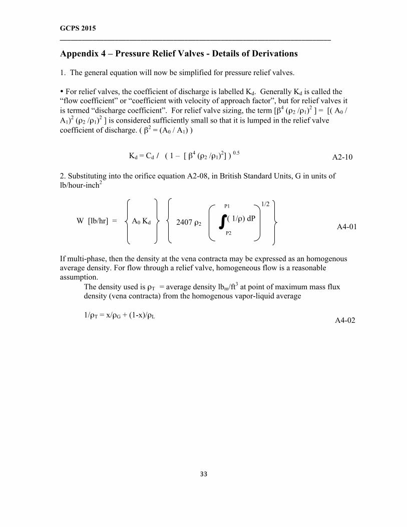
Appendix 4 – Pressure Relief Valves - Details of Derivations 1. The general equation will now be simplified for pressure relief valves. • For relief valves, the coefficient of discharge is labelled Kd. Generally Kd is called the “flow coefficient” or “coefficient with velocity of approach factor”, but for relief valves it is termed “discharge coefficient”. For relief valve sizing, the term [β4 (ρ2 /ρ1)2 ] = [( A0 / A1)2 (ρ2 /ρ1)2 ] is considered sufficiently small so that it is lumped in the relief valve coefficient of discharge. ( β2 = (A0 / A1) )
2. Substituting into the orifice equation A2-08, in British Standard Units, G in units of lb/hour-inch2
If multi-phase, then the density at the vena contracta may be expressed as an homogenous average density. For flow through a relief valve, homogeneous flow is a reasonable assumption.
The density used is ρT = average density lbm/ft3 at point of maximum mass flux density (vena contracta) from the homogenous vapor-liquid average 1/ρT = x/ρG + (1-x)/ρL
A2-10
A4-01
A4-02
( 1 – [ β4 (ρ2 /ρ1)2] ) 0.5
Kd = Cd /
W [lb/hr] = A0 Kd 2407 ρ2
1/2
( 1/ρ) dP P1
P2
∫ P2