Physica D 37 (1989) 270-287 North-Holland, Amsterdam

MODELLING TURBUI~NT MIXING BY RAYLEIGH-TAYLOR INSTABILITY

David L. YOUNGS Atomic Weapons Establishement, A idermaston, Berkshire, UK

Direct two-dimensional numerical simulation and experiments, in which small rocket motors accelerate a tank containing two fluids, have been used to investigate turbulent mixing by Rayleigh-Taylor instability at a wide range of density ratios. The experimental data obtained so far has been used to calibrate an empirical model of the mixing process which is needed to make predictions for complex applications. The model devised, which is a form of turbulence model, is based on the equations of multiphase flow. These equations describe velocity separation arising from the action of a pressure gradient on fluid fragments of different density. The dissipation arising from the drag between the fluid fragments is treated as a source of turbulence kinetic energy which is then used to define turbulent diffusion coefficients. Gradient diffusion processes are thereby included in the model.

1. Introduction

Rayleigh-Taylor instability occurs when a per- turbed interface between two fluids of different density is subjected to a normal pressure gradient, Taylor [1]. If the pressure is higher in the light fluid than in the dense fluid the differential accel- eration produced causes the two fluids to mix. For an overview of work published on Rayleigh- Taylor instability since [1] see the paper by Sharp I2]. One area of current interest is the effect of Rayleigh-Taylor instability on the performance of ~rnertially Confined Fusion capsules. A simple cap- sule might consist of a spherical glass shell with radius of order 100 /~m filled with a deuterium/tritium gas mixture. Laser radiation (or other types of beam energy) is used to implode the capsule. The aim is to obtain sufficiently high temperatures and densities in the DT mixture for thermonuclear reactions to take place. Rayleigh-Taylor instability may occur wherever the pressure-density gradient product Vv" V0 is negative. This will arise at the start c.f the implo- sion at the ablatic,n front between the heated and unheated glass or at the end of the implosion at the gas/glass interface. In either case instability growth tends to reduce capsule performance. Re-

cent work at AWE has investigated the latter case, mixing at fluid interfaces. Ablation front instabili- ties have been studied by many authors, see for example Emery et al. [3].

The term Rayleigh-Taylor instability is some- times limited to the case when the iraterface between the two fluids is subjected to a finite con- tinuous acceleration. A related process, Richtmyer- Meshkov instability [4, 5] occurs when a shock wave passes through a perturbed interface or a nfixed region between fluids of different density. Both processes are important in compressible problems such as the ICF capsule implosion. The present paper will concentrate on Rayleigh-Taylor ir~stability. The Richtmyer-Meshkov process is discussed in this volume by BrouiUette [6] and Besnard et al. [7].

2. Outline of the programme

In real situations the instability will evolve from a multiple wavelength initial perturbation and tur- bulent mixing will occur as suggested by Youngs [8]. Direct numerical simulation of this three- dimensional process is hnpractical except for very

0167-2789/89/$03.50 © Elsevier Science Publishers B.V. (North-Holland Pkysics Publishing Division)

D.L Youngs / Modelling turbulent mLring by Rayleigh- Taylor instabilio, 271

simple cases. Hence turbulence models need to be devised to make predictions for real flows. These models need to be calibrated against experimental results. Experimental studies form an essential part of the AWE programme on this topic.

The programme of work may be divided into three parts:

The computer code solves the incompressible Navier-Stokes equations (pressure-velocity for- mulation) plus an equation for the fraction by volume, fx, of the denser fluid 1:

at + div (flu) = O. (a)

(a) Direct computer simulation of the mixing processes in simple situations. At present 2D com- puter codes are being used. However, in future 3D calculations will be performed. Dir~ , computer simulation has proved to be a useful source of ideas and has played an essential role in planning the experimental programme. It also helps to un- derstand the experimental results.

(b) Experiments. Definitive data on the turbu- lent mixing phenomena come from experimental measurements. An extensive set of experiments on the mixing of incompr~::,;~,ible fluids by Rayleigh- Taylor instability is de~,cribed by Read [9], Read and Youngs [10], Burrow~, Smeeton and Youngs [11] and Smeeton and Youngs [12]. In future, experimental work at AWE will investigate the mixing of compressible gases in shock tube experi- ments.

(c) Turbulence models. The main objective of the programme is to develop turbulence models to represent the mixing processes. These models need to be calibrated against the experimental data. The turbulence models are then used to make predictions for real situations.

3. Direct numedcal simulation

Work began on this study of turbulent mixi~,g by Rayleigh-Taylor instability about ten years ago when a simple 2D finite difference incom- pressible code was written to calculate the growth oi" Rayleigh-Taylor instability ~. a plane bound- ary from a multiple wavelength initial perturba- tion.

The fluid density is then p=f~#~ +(1-f~)o2. Initially the fighter fluid 2 lies above the denser fluid 1, with a body force g per unit mass acting vertically upwards. The initial volume fraction dis- tribution is: fl = 0 for y > ~'(x) and fl = 1 for y < ~'(x) where ~" is the initial perturbation at the interface y = 0. This is given by

n ~ x = sY' .a . cos w

n

for rind frictionless wall at x = 0 and x = W,

o r

2n~rx 2nvx ) ~'(x) = S ~ a,cos - W - + b, sin --W-

for periodic boundary conditions in tile x-direction.

The a,, and b,, are random numbers chosen: from a Gaussian distribution. S is a scaling factor chosen to give the required value nf o = { (~ 2) }l/z. W is the width of the computational region in the x-direction.

The volume fraction transport equation (1) may be solved by a finite difference method which assumes a continuous variation of f~ with posi- tion. The method of van Leer [13] is used to minimise mixing by numerical diffusion. Alterna- tively a front tracking method, Youngs [141. may be used to preserve a sharp interface b :tween the two fluids. Other. more accurate, vorte~ methods for following Rayleigh-Taylor unstable interfaces are described by Tryggvason [15] and Kerr [16]. The front tracking method has been ased for sim~!~' situations such as the growth of t:~e insta- bility from a single wavOength initial :'erturba-

272 D.L. Youngs / Modelling turbulent mixing by Rayleigh- Taylor instability

(a) 2Oms

132 = 0 . 0 3 4

(b) 40 ms

. n r an t ! t m !l : !~t~ ::"-!t:! :!~:~li:~l~[!F!:.n,: : | ! i i | : t , : h t | : ~ i I: i ;] i t l : ~mm:i , t .n . t imi . iu

~(,, Fuiti|in|~fit~fi:3|ii~|milmui:.httt~.mur.tfi:ulutit~it=nl= i*, ~ ~ i i i i l !~ ! i:, F:I i! f l i ~ i ! i~ i i i l !~: !i :J:i:t i l ihil l l i tl :i i l i iit~ ii."l,ii, ' f!! ! i l ! l ! ; . ! ! i i i l l i ! i i l ! l l ! b.!il ~i!i i!, 't i i l i i~i~ l i i i i ;~ i ! i~ i r ih r:i.:.;i l;:i:/i:; l ; ~ l!!:",J !!;! i : i i l ; ;!t

(c) 60 ms

' : r"

I :=~l. i "

;~,n,i~! b..q~ a , r , i ~ ~ ~n n , :ran: :n ".,:t:u:u: :l u :,.: ~:[~llitlitliltilil~.'lililliiliiltlXl~tillillilliit:l=lill:ltllltillitiill

~iili ~lil~l$li$~iiiUi~l!l~i$i.i~i$ll$i$ili$~.iii.~}r~llli !~:i,hli~]=.~[:¢l:lih::l:tt.:,:'fihF.mi!uh~ut~tnih.hi:th*h!~lh=

(d) 70 ms

iiiii!!iii ii!i ii iii iliiii i iiiii iiiiliiliiiii!ii i i i Fig. 1. Two-dimensional simulation with multiple wavelength initial perturbation. Density ratio Pl/P2 = 20. Acceleration g = 0.15 m m / m s 2. Volume fraction contour levels fl = 0.2, 0.5, 0.8.

tion. It is not clear that it improves the accuracy if 1.0, a multiple wavelength initial perturbation is pres- ent. In this case fine-scale (sub-zone) nfixing should indeed occur due to the small scale eddies gener- ated in the turbulent mixing region, which cannot be represented on the computational mesh. Use of the van Leer method for the transport of volume

0 fraction and momentum introduces non-linear nu- -66 merical diffusion into the calculation which plays a similar role to the subgrid eddy viscosity used in large eddy simulation of turbulent flow. The mul- tiple wavelength calculations have used the van Leer method rather than the front tracking method.

An example is shown in fig. 1 which corre- sponds to the experiments described in section 4. The density ratio is Pl/P2 = 20. Periodic boundary, h 1 = a ~ conditions are used. The initial perturbation con- sists of modes with wavelength in the range W/25 to W/8. The width of the computational region is W = t50 mm. The initial perturbation has stan- dard deviation o = 0.025 ram. The size of the computational mesh is 150 x 200 zones.

The numerical simulation shows a short wave- length perturbation of wavelength ---W/25 appearing at early time. At the end of the calcula- tion, the dominant mode has wavelength W/2. Tiffs has evolved from the interaction between shorter wavelength modes. It was proposed by Youngs [8] and confirmed by the experiments of Read [9] that in such circumstances the growth of !he nfixing zone should tend to lose memory of the

1.0 ....... T' l - [ (a) 50 ms

0

height (ram)

(b) 70 ms

Lh2 ___~ " ~ . . . .

+133 -66 0 +133 height(mm)

Fig. 2. Volume fraction averaged over a horizontal layer ver- sus height, for m,qtiple wavelength calculation.

initial conditions and that the depth to which the . . . . . . . . should mi.xJng zone penetrates t_,,c uc:,_,~c,. ,qoid I

be given by

Pl - P2 Pl + P:

gt (2)

2D numerical simulation indicated a - 0.04 to 0.05, whereas experiments suggested a - 0.06 to 0.07;

Fig. 2 shows a plot of f l = ffl dx /W, i.e. the volume fraction averaged over a horizontal layer, versus height y, for the multiwavelength calcula- tion. Measurements of h I (bubble penetration) and h 2 (spike penetration) from these plots indi- cate a = 0.042 and h2/h 1 = 2.3 for this calcula- tion.

The variation of h2/h x with density ratio for the single wavelength perturbation case is shown in fig. 3. The interface tracking method is used. In

D.L Youngs / Modelling turbulent mixing by Ra.vleigh- Tavlor instability 273

(a ) Ol _ ~ - 3

.~-.~1 = 1.7 ~ = 2.9 I

(C) 01 _ 40

~--3.3

Fig. 3. Variation of h2/h I with density ratio. Two-dimen- sional numerical simulation with single wavelength initial per- turbation. Interface plots at nt = 6.

the absence of viscosity or other stabilising mecha- nisms, the growth in the linear regime of the amplitude, a, of a small perturbation of wave- length X is given by [1] / /= n2a, where

n2 2~rg Pt - P2 (3) "- ~k g . t + p 2 "

The initial amplitude used is a 0 = 0.02X. For the thr~e density ratios considered results are shown at times corresponding to the same number of exponer, tial growth periods, i.e. nt = 6. h2/h ~ is a slowly increasing function of #x/Oz. At O~/P2 = 20, h2/h 1 is 2.9, a little more than the value estimated from the multiwavelength calculation, figs. 1 and 2.

The two-dimensional simulatirns suggested that significant instability growth should arise from small random perturbations (via mode coupling) and that the results should fit into a simple pat- tern, h x given by eq. (2 and hz /h x a slowly increasing function of v,/P2. As a result of the numerical sim,..l,~tmns a~, experimental pro- gramme was set up to investigate the true three-dimensional behz:'~eu:. Tb.~ value of the nu- merical simulations lies in the fact that they are an important source of ideas and a stimulus to the experimental programme, rather than m their abil-

ity to make accurate predictions of the mixing phenomena.

4. Experimental results

Experiments on the mixing of two incompress- ible fluids have been performed at a wide range of density ratios using the apparatus described by Read [9]. This consists of an enclosed tank con- taining the two fluids, initially at rest with the lighter fluid 2 on top of the denser fluid 1. The tank is then driven downwards by one or two small rocket motors. The tank is attached to two guide rods which ensure that motion of the tank is vertical. Tank accelerations are in the range 15g0 to 70g o, high enough to ensure that the effects of surface tension and viscosity are small (go = 9.8 m/ s 2 denotes the acceleration due to gravity).

Most experiments have been carried out without any large imposed perturbations, i.e. the aim was to investigate instability growth from small ran- dom perturbations and to confirm tht: gt 2 growth law (2). Details of the experimental results are given in a set of three reports [10-12]. A wide range of fluid combinations has been used, for example:

Liquid/liquid: Nal solution/hexane NaI solution/water

pl//P2 = 3, P l / P 2 = 1.8.

Liquid~gas: alcohol/air (1 bar) pentane/SF 6 (up to 10 bar)

P l / P 2 - - 700,

pl//P2 " 8 tO 30.

Some of the latest experiments [12] used a com- bination of a liquid and a compressed dense gas, SF 6. This enabled density ratios in the ~an~e 8 to 30 to be used where computer sim~qation-see section 3 -,,,,~'"A ,,,,,,,,,,,,~,;~,'; ..... ~ that there was uncer- tainty in the depth to which spikes at hea~' fluid would penetrate the lighter fluid. Photographs for two examples of the pentane/compressed SF6 ex- periments are shown in fig. 4 (01/02 = 8.5) and fig.

274 D.L Youngs / Modelling turbulent mixing by Rayleigh- Taylor instabifiO,

Fig. 4. Pentane/compressed SF 6 experiment. Density ratio Ol/& = 8.5. Acceleration g = 15g e. (a) 32.8 ms. (b) 53.3 ms. (c) 73.7 ms.

5 (Pl/P2 = 29.1). The width of the tank in these and subsequent experiments is W= 150 mm. As the two fluids have very different refractive in- dices, the mixed region appears black on the back- lit photographs. The photographs clearly show the increase in bubble size as time proceeds. The presence of the meniscus at the start of the experi- ment results in a thin film of liquid climbing the tank walls. Also large bubbles form in the tank

comers where the effect of the meniscus is great- est. These effects are ignored when measurements of growth rates are made; h 1 and h 2 are measured on the darkest region in the centre of the tank.

Plots of h x against ( P l - P 2 ) / ( P l + P2)g t2 for these two experiments are shown in fig. 6. Reason- ably good linear correlations are obtained, though for the higher density ratio experiment there is some slowing down of the growth rate at late time

Fig. 5. Pentane/compressed SF 6 experiment. Density ratio &/P2 = 29.1. Acceleration g = I5g o. (a) 33.5 ma. (b) 56.9 ms. (c) 67.3 ms.

D. L Youngs / Modelling turbulent mixing by Rayleigh- Tm,ior instabilitr 275

E 40" E c" ._o 30-

=e-20- (13 o.

10. .13 .13 m U

®-~2=8.5, o~=0,072 . ~ / ' ~ ~ " x

0 100 200 300 400 500 600 700 0 1 - 0 2 u'~t2, mm ,Ol + 02

Fig. 6. Bubble penetration versus scaled acceleration distance for two pentane/compressed SF 6 experiments.

which may be due to the dominance of the large comer bubbles at this stage. The values of a for these two experiments are 0.072 and 0.060.

has been measured for about 50 of the experi- ments described in refs. [10-12]. The values ob- tained lie in the range 0.050 to 0.077. There is no noticeable variation with density ratio. Some of the experiments were of better quality than others. If this is taken into account, the recommended value is a = 0.06 for all density ratios.

The variation of h z/h~ with density ratio is shown in fig. 7. As predicted by the numerical simulations h 2/h~ is a slowly increasing function of #~/P=- At #x/#~ = 20, the experimental. 'sults give hz/h~ = 2.0, a little less than the value of 2.3 indicated by the multiwavelength numerical simu- lation, fig. 1.

fl c ©

t - ¢- Q)

r3 i1~

Im

2.5

2.0

1.5

1.C

® f

e.N s

s , ~ s ®

®.-'*x ® Pentane/SF6

/" ® x Water/SF 6 /

¢ • Nal solution/ I ' Pentane t

f 1 10 2'0 30 40

Density ratio 01[02

Fig. 7. Experimental variation of h2/h I with density ratio.

In some experiments the fluids used were CaC12 solution and hexane with the CaC12 concentration adjusted so that the two fluids had the same refractive index. The density ratio obtained is P~/O2 = 1.73. The CaC1 z solution is dyed and the backlighting made as uniform as possible. The fluids then act as pure absorbers of the backlight and the film density, at, on the photographic nega- tive may be related to the amount of dyed fluid. The dye level is chosen so that d varies linearly with f~ in calibration tests. Then for the experb ments

d m a x ~ d

f~ = dm~,- dmi~'

where d ~ , is the film density at the top of the tank (pure fluid 2) and d~j, is the film density at the bottom of the tank (pure fluid 1). Fig. 8 shows

Fig. 8. Experiment using fluids with matched refractive indices. CaCI 2 solution (dyed) /hexane (clear~. Density ratio

Acceleration g = 43g o. (a) 0 ms. (b) 63.0 ms. (c) 73.9 ms.

o , / ~ = 1 7 3

276 D. L Youngs / Modelling turbulent mixing by Rayleigh- Taylor instability

1.0"

0.5

1.0"

0.5

-~o

(a) 57.5 ms X X

X

X X

X X

X

6 +50 Height, mm

-gO

%

(b) 73.9 ms

\ %

" 6 ..... "

Height, mm

Fig. 9. Volume fraction averaged over a horizontal layer ver- sus height for the experimem shown in fig. 8.

photographs for one of the matched refractive index experiments. Fig. 9 shows plots of ft, i.e. fl averaged over a horizontal layer, versus he i s t . The sLape obtained is in reasonable agreement with that expected from 2D numerical simulation. However, the experimental profile should be re- garded as approximate because of the difficulty in achieving perfectly uniform backlighting and in matching the refractive indices exactly.

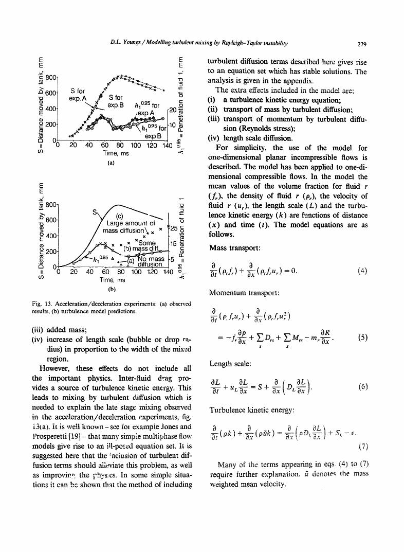
For lhe two experiments described in [12] the tank was first accelerated as usual and then, when the rocket motor had burnt out, was decelerated cy springs. In the final stage the tank moved vemcally upwards with near constant vel,ocity~ These ex,',~,q,-~-~t~. ~.~,, :~ocl ~h~ CaC!~ solution/ hexane combination. 1he but~ble penetration /~, sbown in fig. 13(a), was deduced from the f profile, h t was measured to the point where f~ = 0.95. During the acceleration phase h~ increases as expected. During the deceleration phase h~ de- creases, i.e. partial de-mixing occurs. In the final coasting phase the mixed region grows again. It is

shown in the next section how the late time be- haviour may be modelled by a combination of pressure gradient and turbulent diffusion effects.

Some experiments described in il l , 12] used three layers of liquid, carbon tetrachloride/NaCl solution/hexane, with densities Pl > P2 > Ps- The density of the intermediate layer was chosen so that P2 = J(PtP2), i.e. the Atwood number was the same at the two interfaces. The initial thickness of the intermediate layer A varied from 5 to 20 ram. However, it proved difficult to obtain good results with zl = 5 ram; the meniscus on the top and bottom of the layer appeared to affect the results. The aim of these experiments was to quantify the reduction in the mixing of fluids 1 and 3 due to the intermediate layer. In order to obtain results in a non-dimensional form 6/A is plotted (see fig. 16(a)) against ( 01 - P2)/(Pt + P2)gt2/A where the width of the mixed region 8 (which equals A at t = 0) is the distance between the boundary of the unmixed fluid 1 and the boundary of the unmixed fluid 3. At early times the rate of growth of 6 is about half that expected without the intermediate layer. This is consistent with the reduced initial Atwood number. However, even when 8 - 5A long after the intermediate layer is fully mixed the growth rate appears to be significantly reduced by the effect of the intermediate layer.

In several experiments the tank and guide rods were inclined at an accurately measured angle, 0, to the vertical. The acceleration g remained paral- lel to the tank sides and the initial interface was inclined at an angle 0 to the direction of accelera- tion. The inclination of the initial interface results in a gross overturning motion in addition to the fine scale rmxing. This .gives a flow which is on average two-dimensional from precisely known initial conditions and provides data for testing future two-dimensional versions of the turbulence model described in the next section. Results for two such experiments are shown in figs. 10 i p , / p ,

\ • , t . ~ . .

= 3) and 11 (Px/P2 = 20). At •x/p2 = 3 a large bubble of fluid 2 penetrates the heavier fluid at the right-hand side of the tank. A similar structure forms on the left-hand side of the tank. This grows

D.L Youngs / Modelling turbulent mixing by Rayleigh- Taylor iltstability 277

! ~ ! i ; ~ / ~ i ~ i ~ i ~ ~ i ! ~ ! ! i ~ ! ; ! i i , ~ ; i ~ ? ! ¸̧ i i / : i

: : : i i H e x a n e ~ ~ ~

..... , ~ i i / ~ m ~ ~̧!̧i~i̧~̧~̧~' ; ~ i m R~i~i~i~i~i~!!ili!~ ~i! . . . . . . . . . . . . . . . • ;~! ~~!!~'~i~ii!!iiii~i ~ i :̧ ̧~̧:̧ ̧............. ! :~̧¸̧ ? !i ~'!~' ~̧~':~!~̧!~;̧!; Nal solution . . . . .

Fig. t0. NaI solut ion/hexane experiment. Rig tilted by 5 ° 46', Density ratio Pl/O2 = 2.9. Acceleration g = 35go. (a) 35.7 ms. (b) 54.9 ms. ~c) 71.1 ms.

iii~ii:i//!~ ~! ii!~ii~ ' ~,~!i~!: ̧I; . . . . . . i ~!i!!i!i!i .......

iiiii~i!:~::! ~ . . . . ~ i~ii'!iiii~i~ill ii~ ii:ill !

Fig. I1. Pentane/compressed SF 6 experiment. Rdg ~iRed by 5 ° 9'. Density ratio #~/~'2 - 19.6. ..-~,_,.,,,,,,.o, ~ ........... 8 = itgu. ~.q 31.2 ,,~. (b) 42.3 ms. (c) 52.9 ms.

278 D.L Youngs / Modelling turbulent mixing by Rayleigh-Taylor instability

(c) 0:/02 = 20,

t = 3 0 ms

i l l ~' , I ¢.. •

ill ii ........ ' .............. I

! !i! ! ! kq ! l l ! ! I ! ! ! ! I ![!'-"!l!.i! i ! ! !,:R! ! ! I ! ! ! ! ! ! l ! i ! ! ! ! ! f i I ! ! III i i i i i i i i i ! i l i i i i l i i i i i i i i i l i i i i l i i l i i l i l i i i i l i

i i i I i ! i i l i i i ! I i ! ! i .:-i'.'! i i l l ! i i i t i i ! i i • " . ' i , ~1 . . . . . . ~ .... • : . . . . . ~ . . . . . . ~:i!:ll:ml!t :u. : li..m: u: i:lili}lt!li:i:i!ilit!i, i . i ;hi : it :

\/ t - 6 0 ms

I ,-~

i i i i i i i i i i i~ . ih ' r ~ !1~ \ iiiiiii % ..f& l l i t ! i t i t l i ! : - " l i | ! l b :'." :4,

nl l l / l l l l l l l t l l l l l i l f : l l l l i l : : i l l l : l . I I l~:: l l : ; : l : l l l l : "~ I I ~ " ~, i i i i | ' | i i ' i i i i i ' i l l i l i ~ i l l ;~ i~ i~ i i i i~ i [ i i i i l l :q i:'i!i.P" '~

l l l l l l l l l l l l l i i l i l i i i l i l l ! . ' . ' i i ! i.'1 li.:!i:!i l '~i !L'. " , i ! i ! i l l ! "~! ~ !~! f i ! ~ iE! i~!; i !~ll i

~liiiiilil;iil;i~iiilTt:~:i:';;!"i:T!i~'i!!!~}

l iiiiiiiiiiiiiiiiii:iiiiiiiiiiik / ~ , !~ i i i i ! i i i ! i i i i i i ! ~ i i i i i i i i i ! ! i ! i i i i i ! i i i i i i i i i i i i i t i ~ : ~

Fig. 12. Two-dimensional numerical solution of t"e tilted-rig experiments. Volume fraction contour levels, fl = 0.2,0.5,0.8.

a little faster. At 101/102 = 20, the behaviour is significantly different. In this case a thin spike of fluid 1 forms at the left-hand side of the tank. Results of two-dimensional numerical simulation of these two experiments are shown in fig. 12. Rigid frictionless walls were used at x = 0 and x = W. The initial perturbation consisted of a combination of cosine modes with n = 31 to 50 and o = 0.025 nun (see section 3), superimposed on the tilted interface. The simulations reproduce the behaviour of the observed features at the sides of the tank. This shows that neither wall frictio, nor the presence of the meniscus has a w.ajor effect on the development of these features. The fine scale mixing in the centre of the tank appears to be underestimated in the simulations. It is likely that three-dimensional simulations would be needed to calculate this correctly.

5. Turbulence models

5.]. "tr'l~e m '''4or e~,.L,':,.Ho~e

Turbulence models are needed to predict the average mbdng behaviour in ~,ows ttat are on average one- or two-dimensional. The approach to the ,,onstruction of tile turbulence model is guided by the experimental behaviour. The photog~aphs in figs. 4 and 5 clearly show bubbles of gas pene-

trating the denser liquid. At any given time there appears to be a characteristic bubble size which increases as the mixed region develops. Instead of using closure laws for fluctuating quantities, as is done in many turbulence models, the present model is based on representing the dynamics of the observed structures in the mixed region (bub- bles of light fluid or drops of dense fluid). The need to model the motion of bubbles or drow in a pressure gradient suggests using the equations of multiphase flow. A simple two-phase flow model for Rayieigh-Taylor instability was described by You~gs [8]. Tile pre~,za: p~per considers the exten- sion to many fluids and the addition of extra physics. Two-fluid turbulence models have been widely used by Spalding and were applied to mixing of fluids by Rayleigh-Taylor instability in [17]. Andrews [18] has considered the extension of a simple two-fluid model for Rayleigh-Taylor instability to two dimensions. Alternative ap- proaches for the Richtmyer-Meshkov case are described in these proceedings by Besnard et al. [7!.

The present multiphase flow ,ncdet represents the following effects: 0) differentma acce!ere.fion induced by the pres-

sure gradient on fluid fragments of different densities;

(ii) drag between fluid fragments, proportional to velocity difference squared;

D.L. Youngs / Modelling turbulent mixing by Rayleigh- Taylor instability 279

E E

~" 800

-~ 600 13

400- E

o 200" e -

.m m 0 II

03

E E

I " "

,~al:x'L-_-o,

S for i ~ "x~'g~'l'x'~'~" 5 exp.A .z? S for "6

" ~ . . . . . exp.B hl 0.9s for / exp.A [ 2 0 ~

• ~ p. [ m II 20 40 60 80 100 120 140

Time, ms "~- (a)

E E

S of_ , 600-

oe> .__1 / mass di f fusion\ x x :25 = 4UOJ / x -

x / / e x ~ x x ..x *Some, .15

/ " ; mass " <.o i ~t-i" -nc - - ° .-:---(a)~F, . ~ -o II t-- ...*~'" " ~ K" affrUSlOn

,, O0 20 40 6'0 8'0 160 120 140 o_ co Time, ms 4:

(b)

Fig. 13. Acceleration/deceleration experiments: (a) observed results, (b) turbulence model predictions.

(iii) added mass; (iv) increase of length scale (bubble or drop ra-

dius) in proportion to the width of the mixed region.

However, these effects do not include all the important physics. Inter-fluid drag pro- vides a source of turbulence kinetic energy. This leads to mixing by turbulent diffusion which is needed to explain the late stage nftxing observed in the acceleration/deceleration experiments, fig. i31a~, it is well known - see for example Jones and Prosperetti [19] - that many simple multiphase flow models give rise to an ill-posed equation set. It is suggested here that the !nch~sion of turbulent dif- fusion terms should alleviate this problem, as well as impro~@.-, the rhys, cs. in some simple situa- tions it can be shown that the method of including

turbulent diffusion terms described here gives rise to an equation set which has stable solutions. The analysis is given in the appendix.

The extra effects included in the model are: (i) a turbulence kinetic energy equation; (ii) transport of mass by turbulent diffusion; (iii) transport of momentum by turbulent diffu-

sion (Reynolds stress); (iv) length scale diffusion.

For simplicity, the use of the model for one-dimensional planar incompressible flows is described. The model has been applied to one-di- mensional compressible flows. In the model the mean values of the volume fraction for fluid r ( f r), the density of fluid r (Or), the velocity of fluid r (Ur), the length scale (L) and the turbu- lence kinetic energy (k) are functions of distance (x) and time (t). The model equations are as follows.

Mass transport:

~--7(Orfr) + (PrLUr) =0. (4)

Momentum transport:

+

~p ~R = --fr"~ + EDrs + E M r s - mr •X"

.¥ S

(5)

Length scale:

~t + UL-~- = S + DL-~ . (6)

Turbulence kinetic energy:

+ S A -{.

(7)

Many of the terms appearing in eqs. (4) to (7) require further explanation. ~ denote~ lhe mass weighted mean velocity.

280 D.L. Youngs / Modelling turbulent mixing by Rayleigh- Tayior instability

Mr~ represents the added mass for fluid r due to fluid s. This is given by

The source term in the length scale equation (6) is

(D, ur M~, = - 0 . s p j , f~ o t

D,.u,. ~u, a~t,. D--T- = --~i- + u ,

D~U s ) Dt , where

is the acceleration of fluid r and

p,,=(/,p,+f~p,)l(/,+/~).

(8)

This is an extension to many fluids of one of the formulae for two-fluid flow analysed in [19]. The coefficient 0.5 is chosen to give the correct added mass for isolated spherical particles of fluid r surrounded by fluid s.

D,~ denotes the drag on fluid r due to fluid s and is given by

p,,Lf, O , , = - c t L lu,- u,- wr+ Wsl

x ( , , - , , - w,+ w,). (9)

The drag coefficient c t is obtained by matching experimental data, as will be explained in the next section, w r is the value of u r - ~ expected if mixing is enth'ely due to turbulent diffusion. denotes the volume weighted mean velocity. In that case mass flow is given by

with mean density p = Ef , Pr. This can be inter- preted as fluid r mass flux:

whence

D

with D = turbulent diffusion coefficient. When the drag coefficient c 1 ~ c~, u , -

w , - w+ as requh'ed.

/"+}: St. = E f f f , p, + p, (u s - u ,) fff.~. (10)

r > $ x

The fluids are numbered r = 1, 2, 3,.. . in order of increasing initial position. Then SL > 0 if the nuids are mixing and St < 0 if the fluids are de-mixing.

For two fluids

20 }t/2 s , = pt + p2 (ul - u2).

This form is chosen to give an approximately uniform length scale, proportional to the width of the mixed region. Eq. (10) is simply a plausible extension of the two-fluid formula.

For the two-fluid case the advection velocity in the length scale equation is

u , = a + ( A - / x ) ( u x - u,).

This formulation, due to Andrews [18], trans- ports the length scale away from the centre of the mixed region and was found to improve the stabil- ity of the solution. For the multifluid case u L is obtained by a plausible extension of the two-fluid formula:

The term - m r OR/ax in the momentum trans- port equation, where mr=frpr /p is the fluid r mass fraction, represents the effect of the Reynolds stress. The use of the mass fraction in this term will be explained later. As in turbulent diffusion models such as the (k, e) model, see for example Leith [20], the Reynolds stress in one-dimensional planar geometry is given by

D.L Youngs / Mcdelling turbulent mixing by Rayleigh-Taylor instability 281

with Travis et al. [22], may be obtained by setting

i.Lt --- pkl /21t '

I t = turbulence length scale.

The turbulence kinetic energy equation (7) is also the same as that used in turbulent diffusion models. The dissipation rate is

p!:3/2 c = 0.09 it .

The coefficient 0.09 is an appropriate value for turbulent shear flow models, see Launder and Spalding [21]. However, it should be pointed out that there are no experimental measurements of the dissipation of k in Rayleigh-Taylor mixing. The turbulent diffusion coefficients D and D k are the same as for turbulent shear flow [21], i.e. D = 2kl /21 t (mass diffusion)and D k = kl/21t (k- diffusion). In the length scale equation DL = 2k l /E l t is used.

The source term in the turbulent kinetic equa- tion (7) is

0fi S , = E ( u ~ - U r ) ( M , , + . ~ ) - R ~ .

r < s

The turbulence length scale is assumed to be proportional to the fragment size L. Two model constants now remain which need to be chosen ~o fit data on Rayleigh-Taylor mixing. These are

c~ = drag coefficient, determines the overall mixing rate,

c 2 = l u l L , determines the relative importance of turbulent diffusion and pressure gradient effects.

In order to check that turbulent diffusion effects have been incorporated in a plausible manne~ it is worthwhile examining a simple firnifing case, the drift-flux approximation for two-fluid mixing. This is valid when the inertial effects on the velocity separation u 1 - u z are negligible and, following

D~u~ D2u 2 Dt De "

The added mass terms vanisk and equating the fluid accelerations gives

1 0 p Dxz 1 ~)R ax + +

1 0 p D21 P2 OX + P---~f2

1 OR a-;'

with

D12 = -- D21

caof, f, L [ U l - I'/2 "1- W 1 -- W21

×(ua-u,_+ w2),

whence

{ L [ P,. - P2 ~p [)1/2 bl I -- bl 2"- S -~1 p2 ~X q" Wi - W2

= pressure diffusk~n t e ~

+ gradient diffusion term,

3p S = s i g n { ( # l - P 2 ) ~-~)-

A plausible result is obtained. Velocity separa- tion is due to a combination of pressure diffusion and gradient diffusion effects. As a result of using the mass fraction m r in the Reynolds stress term in eq. (5), the Reynolds stress terms cancel and the velocity separation due to turbulent diffusion is, as required, given by the wx - w 2 term.

There is one major omission in the present model. In many of the applications, such as the ICF implosion referred ~o h~ the i~troduction, the fluids involved will be qaiscible and, as a result of the presence of small scale eddies in the turbulent mixing zone, will to some extent mix at a molecu- lar or atomic level. This will have many effects. The density differences on which the pressure gra-

282 D.L Youngs / Modelling turbulent mixing by Rvvleigh- Ta3'lor instability

dient acts will be reduced. Mixing at a molecular level will inhibit the de-nfixing which will occur if the acceleration changes from the unstable to the stable direction. It is planned to model these ef- fects by an exchange of mass between the fluids. However, the model would need to be calibrated against experiment and there is at present no observed data on the degree of molecular or fine- scale mixing in Rayleigh-Taylor unstable flows.

5.2. Application of the model

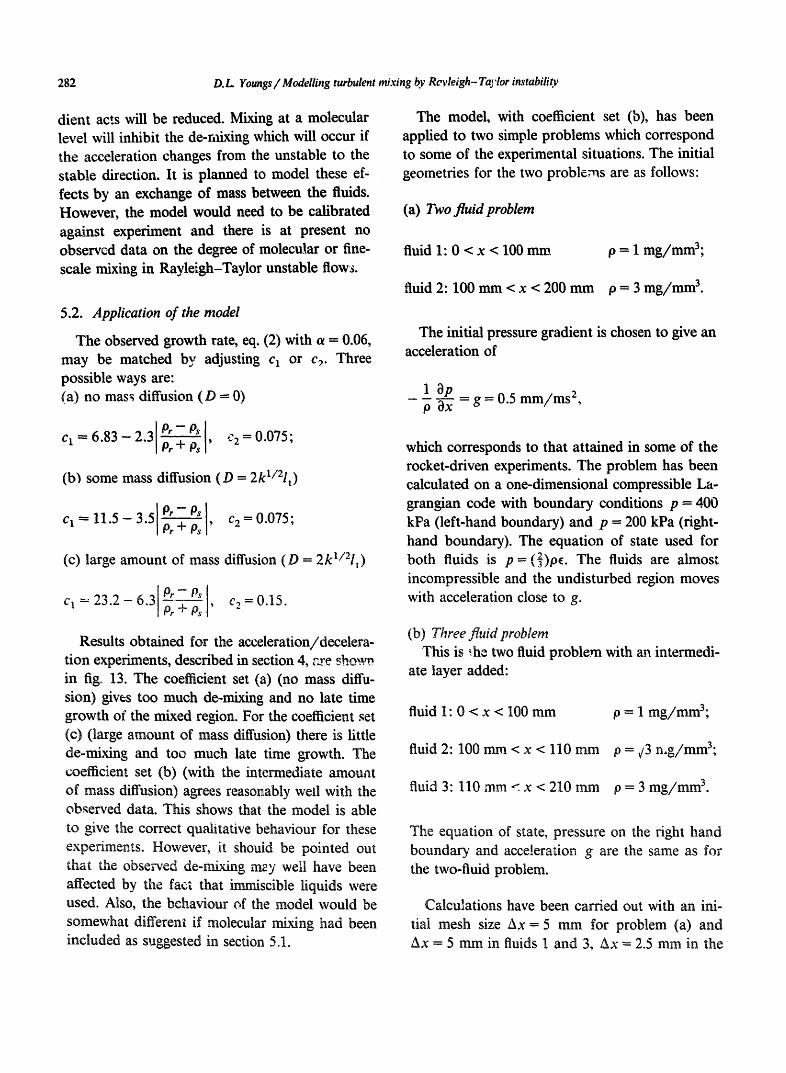
The observed growth rate, eq. (2) with et = 0.06, may be matched by adjusting c 1 or c~. Three possible ways are: (a) no mass diffusion (D = 0)

cl -- 6.83 - 2.3 #,-+ 0s ' c2 = 0.075;

(b~ some mass diffusion ( D - 2kl/21t)

c~ -- 11.5 - 3.5 0r + 0s ' c2=0"075;

(c) large amount of mass diffusion ( D - 2U/21,)

c 1 --" 23.2 - 6.3 ~--~p~ , c: = 0.15.

Results obtained for the acceleration/decelera- tion experiments, described in section 4, ere showp in fig. 13. The coefficient set (a) (no mass diffu- sion) gives too much de-mixing and no late time growth of the mixed region. For the coefficient set (c) (large amount of mass diffusion) there is little de-mixing and too much late time growth. The coefficient set (b) (with the intermediate amouat of mass diffusion) agrees reasonably well with the observed data. This shows that the model is able to give the correct quafitative behaviour for these experiments. However, it shouid be pointed out that the observed de-mixing may well have been affected by the fact that immiscible liquids were used. Also, the bchaviour of the model would be somewhat different if molecular mixing had been included as suggested in section 5.1.

The model, with coefficient set (b), has been applied to two simple problems which correspond to some of the experimental situations. The initial geometries for the two problems are as follows:

(a) Two fluid problem

fluid 1 :0 < x < 100 mm p = 1 mg/mm3;

fluid 2:100 m m < x < 200 mm p = 3 m g / m m 3.

The initial pressure gradient is chosen to give an acceleration of

1 0p P 0x = g = 0.5 m m / m s 2

which corresponds to that attained in some of the rocket-driven experiments. The problem has been calculated on a one-dimensional compressible La- grangian code with boundary conditions p = 400 kPa (left-hand boundary) and p = 200 kPa (fight- hand boundary). The equation of state used for both fluids is p = ( ~ ) p c . The fluids are almost incompressible and the undisturbed region moves with acceleration close to g.

(b) Three fluid problem This is ~he two fluid proble~ with an intermedi-

ate layer added:

fluid 1 :0 < x < 100 mm p = 1 rag/ram3;

fluid 2:100 mm < x < 110 mm p = ¢3 n.g/mm3;

fluid 3:110 m m < x < 210 mm p = 3 m g / m m 3.

The equation of state, pressure on the right hand boundary and acceleration g are the same as for the two-fluid problem.

Calculations have been carried out with an ini- tial mesh size ax = 5 mm for problem (a) and Ax = 5 mm in fluids 1 and 3, Ax - 2.5 mm in the

D.L. Youngs / Modelling turbulent mixing by Rayleigh- Taylor instabili~ 283

(a) Volume fractions

/ •

90~'--- x(mm) 1105 (b) Turbulence

kinetic . ~ ' ~

k

903 x(mm) 1105 (c) Length scale

L

303 x(mm) 1105

I(a) Volume fr!~iions

fr

901 x(mm) 1112 (b) Turbulence

kinetic ~ ' ~

k

901 x(mm) 1112

901 ×(ram) 1112

Fig. 14. Turbulence model results for the two-fluid woblem at t = 60 ms.

Fig. 15. Turbulence modcl results for the three-fluid problem at t = 60 ms.

thin intermediate layer for problem (b). Plots of f , , L and k against x are shown in figs. 14 and 15. Fig. 16(b) shows a plot of 8, the width of the mixed region against gt 2, for problems (a) and (b).

is defined as the distance between the points where ft = 0.95 and fz =0.95 (problem (a)) or ft = 0.95 and f3 = 0.95 (problem (b)). For problem (a) 8 varies finearly with gt z. However, the straight line does not pass through the origin. Extrapolat- ing back to t = 0 gives ~--1.2 Ax at t = 0. This ~,~ight overshoot is due to numerical diffusion in the solution of the "~olume fraction transport equation. The method used for volume fraction transport is derived from the high-order mono- tonic advection method of van Leer [13]. If first ~rder, upwind differencing had been used the nu- merical error would have been far greater.

Tbe effect of the intermediate layer on the growth rate of the mixed region agrees well with the experimental results shown in fig. 16(a).

6 . C o n c l u s i o n s

Direct numerical simulation gives insight into the way fluids mix by Rayleigh-Taylor instability in idealised situations. Simple laboratory experi-

process indicated by numerical simulation and have provided good estimates of the growth rate of the turbulent nfixing zone at a wide range of density ratios.

In order to make predictions for real applica- tions an empirical model of the mixing processes

284 D.L. Youngs / Modelling turbulent mixing by Rayleigh- Taylor instabifiO,

(a) Experimental results

6 Width of mixed region ~o'& ~ ~ = ~ w ] - d ~ n ~ l a y e r ,~.~^ ~,,'o.'~ e

4. ,o11 ~5" ~ ~ "x '+ '~t4:" ,x+}&=20 mm

2 I . . ~ " " " , ,®}& = 10 mm 0 .'-~" . . . . . . . . . .

10 20 30 40 50 60 70 80 90 100 p l - p3 gt21A 01 "tP3

(b) Multifluid model predictions

Width of mixed region = Initial width of intermediate lav-"~" .x/

12- j 10- Two fluid problem • • x J

[A = m - 0 2 1 " ' , / .,.-,..

6-

4- ~x~, . . . . . . .~ - i x= 10 mm

2- / ~ + o'--"3

0 - lc 2'0 3'0 40 5'0 6'0 70 8'0 9'0 llJ0

Agt 2 ,&

pated into heat and the extent to which the fluids mix at a molecular level. Several research labora- tories are at present investigating the mixing of gases of different densities in shock tube experi- ments. The data obtained from these experiments will play an essenti~ role in validating the model in compressible situations.

Appendix

Stability of the model equations

It is well known (see for example Jones and Prosperetti [19]) that the multiphase flow equa- tions, described in section 5.1, with turbulent diffusion effects omitted, give rise to vnstable solu- tions. By using the sa,:~e type of perturbation analysis as described in t19], it is shown here that tll¢ addition of turbulent diffusion terms removes the problem in a simple two-fluid case. Reynolds stress terms, which have negligible effect on the one-dimensional incompressible problems consid- ered here, are omitted as they complicate the analysis. The equations considered are: Volume fraction:

Fig. 16. Width of mixed region versus scaled acceleration dis- tance for two-fluid and three-fluid experiments: (a) observed results, (b) turbulence model predictions.

0t + ( f r " r ) = 0" (A.1)

needs to be devised. It has been shown that the multiphase flow equations with turbulent diffusion terms added provide a suitable framework for such a model. The equations model the mixing of fluids arising from the action of a pressure gradi- ent on fluid fragments of different densities, as well as mixing by gradient diffusion. The empirical model needs to be calibrated against observed data. The experimental results obtained so far provide a good basis. However, there are some gaps in the measurements such as the proportion of the turbulence kinetic energy which is dissi-

Acceleration:

Drur Op f~o, Dt - - £ - ~ + Mr, + Dr, + Long, (A.2)

VVIUl r = I , 2 - - - ~ ~tnu S ,-¢- r. The added mass terms are

Dlul D2uz ) MI2 = -- M21 = --caflf2P DI Dt '

where c a = 0.5 is the added mass coefficient, and

D.L. Youngs / Modelling turbulent mixing by Rayleigh- Taylor instabilio, 285

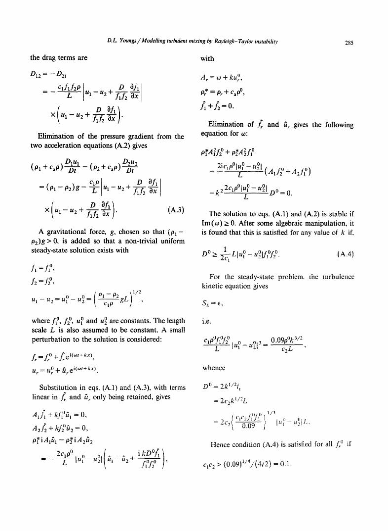
the drag terms are with

D12 = _ D21

- L ul - u2 + fafz Ox

X u x - u 2 + / l f 2 Ox "

Elimination of the pressure gradient from the two acceleration equations (A.2) gives

Dxux D2u2 ( o, + c.o ) o , ( o~ + c.p ) Dt

¢1o[ = ( P l - - P 2 ) g - - T u l - u2 +

( O ,l) X u l - u 2 + flf2 Ox "

AA Ox

(A.3)

A gravitational force, g, chosen so that ( 0 1 - P2)g > 0, is added so that a non-trivial uniform steady-state solution exists with

f~=fa °,

A=~, Ul __ U2 __ lgO_ gO = P! -- P2 gL

Cl p

A r = w + ku °,

p* = o, + c~o °,

Elimination of f~ and ~, gives the following equation for o~:

p , A2¢O t~.d2¢0 1--alJ2 + V2~'x2J1

2ic , oOlu o - uOl - T ¢ ~.o ~.oXlA,ji+Azlf)

_ k 2 2 q O ° l u ° - u°l DO=0. L

The solution to eqs. (A.1) and (A.2) is stable if Im(~o) >__ 0. After some algebraic manipulation, it is found that this is satisfied for any value of k if,

1 D O > ~ LI u° - uOlfOf2 °. (A.4)

For the steady-state probiem, the turbulence kinetic equation gives

S = ~ k

where fo, fo, u o and u ° are constants. The length scale L is also assumed to be constant. A small perturbation to the solution is considered:

f r = frO + ~ e iO't+kx),

tl r -- blot + ~r ei(wt+kx)

i.e.

o 0 0 0.09pOk3/2 c'P fi'fz~ [u o_ u°13= L " c2L

whence

Substitution in eqs. (A.1) and (A.3), with terms ^ ^

linear in f, and u, only being retained, gives

^ O^ All1 + kf~ u~ = O,

^

A 2 f 2 + k f ~ u 2 = O ,

p~iAlUl -- P2 IA2u2

2qP° ( - L lu ° - u ° l ~ - ~ 2 "

i kD°j~ ) f? /o ,

DO= 2kl/2lt

= 2c2k t /2L

roe0 1/3 ( C1C2Jlj2 ) ,H~I ' - H~,L.

= 2c2 0.09

Hence condition (A.4) is satisfied for all f o if

c,c 2 > (0.09)'/4/(4¢2) = 0.1.

286 D.L. Youngs / Modelling turbulent mixing by Rayleigh- Taylor instability

The preferred coefficient set (b) of section 5.2 has q c 2 = 0.86 for small density differences and ctc 2 = 0.60 for large density differences. Hence for the simple situation considered here the turbu- lence model has stable solutions.

It is interesting to compare the results obtained here with the methods used by other authors to obtain an equation set with stable solutions. Two- pressure models have been widely used for this purpose; see, for example, Stuhmiller [23], Hancox et al. [24] and Ransom and Hicks [25]. In such models each fluid has its own pressure, Pr, and the pressure gradient term on the fight-hand side of eq. (A.2) is modified as follows:

3p .3p~ a L (A.5) - L - g ; - - " - - f f - ( P , - P ) a x .

/3 denotes the interface pressure. In the present model, if the turbulent diffusion term is treated as a small correction, the drag on fluid 1 becomes

c AAo Dt2- L lua-u21(ul-u2)

2q0 L l u l - u21D 3x "

Then if the limiting value (A.4) is used for D, the effect is to add the term

aL -oAf,.(u -u2)2Ox

to the fight-hand side of (A.2). As in the two-pres- sure models a term proportional to the volume fraction gradient is introduced. The result ob- tained is similar to the two-pressure model given in [23, 24] for bubbly or droplet flow (fl small) which uses

Pl =P2 =P,

P -- P -" Cp02(~/1 -- U2) 2'

where Cp = dynamic pressure coefficient.

The pressure difference is derived by consider- ing the flow past a sphere.

Hence the inclusion of turbulent diffusion terms as described in section 5.1, although obtained by very different physical reasoning, bears a strong resemblance to two-pressure models.

References

[1] G.I. Taylor, The instability of liquid surfaces when accel- erated in a direction perpendicular to their planes. I, Proc. Roy. Soc. A 201 (1950) 192.

[2] D.H. Sharp, An overview of Rayleigh-Taylor instability, Physica D 12 (1984) 3.

[3] M.H. Emery, J.P. Dahlburg and J.H. Gardner, The Rayleigh-Taylor instability in ablatively accelerated tar- gets with 1, ½ and ¼/~m laser fight, Phys. Fluids 31 (1988) 1007.

[4] R.D. Richtmyer, Taylor instability in shock acceleration of compressible fluids, Commun. Pure Appl. Math. 13 (1960) 297.

[5] E.E. Meshkov, Izv. Akad. Nauk. SSSR, Mekh. Zhidk. Gaza 5 (1969) 151.

[6] M. Brouillette and B. Sturtevant, Growth induced by multiple shock waves normally incident on plane gaseous interfaces, these Proceedings, Physica D 37 (1989) 248.

[7] D. Besnard, J.F. Haas and R. Rauenzahn, Statistical mod- elfing of shock-interface interaction, these Proceedings, Physica D 37 (1989) 227.

[8] D.L. Youngs, Numerical simulation of turbulent mixing by Rayleigh-Taylor instability, Physica D 12 (1984) 19.

[9] K.I. Read, Experimental investigation of turbulent mixing by Rayleigh-Taylor instability, Physica D 12 (1984) 45.

[10] K.I. Read and D.L. Youngs, Experimental investigation of turbulent mixing by Rayleigh-Taylor instability, AWRE Report 0-11/83 (1983).

[11] K.D. Burrows, V.S. Smeeton and D.L. Youngs, Experi- mental investigation of turbulent mixing by Rayleigh- Taylor instability, II, AWRE Report No. 0-22/84 (1984).

[12] V.S. Smeeton and D.L. Youngs, Turbulent mixing by Rayleigh-Taylor instability¢ III, AWE Report No. 0- 35/87 (1988).

[13] B. van Leer, Towards the ultimate conservative ctirl~rence scheme: IV, a new approach to numerical convection, J. Comp. Phys. 23 (1977) 276.

[!4] D.L. Youngs, Time-dependent multi-material flow with large fluid distortion, in: Numerical Methods for Fluid

Press, New York, 1982). [15] G. Tryggvason, Numerical simulations of Rayleigh-Tayl.or

instability, J. Comp. Phys. 75 (1988) 25L [161 R.M. Kerr, Simulations of Rayleigh-Taylor flows using

vortex blobs, J. Comp. Phys. 76 (1988) 48. [17] D.B. Spalding, A turbulence model for bouyant and corn-

busting flows, Int. J. Multiphase Flow 24 (1987) 1.

D.L Youngs / Modelling turbulent mixing b.v Rayleigh- Taylor instability 287

[18] M.J. Andrews, Turbulent mixing by Rayleigh-Taylor in- stability, Imperial College Report CFDU 86/10 (1986).

[19] A.V. Jones and A. Prosperetti, On the suitability of first- order differential models for two-phase flow prediction, Int. J. Multiphase Flow 11 (1985) 133.

[20] C.E. Leith, Coherent structures in a turbulence model with stochastic backscatter, unpublished.

[21] B.E. Launder and D.R Spalding, Mathematical Models of Turbulence (Academic Press, New York 1972).

[22] J.R. Travis, F.H. Harlow and A.A. Amsden, Numerical

calculation of two-phase flows, Nucl. Sci. Eng. 61 (1976) 1.

[23] J.H. Stuhmiller, Influence of interracial pressure forces on the character of two-phase flow model equations, Int. J. Multiphase F ! ~ 3 (1977) 551.

[27] W. i'. Hancox, R.L. Ferch, W.S. Lui and R.E. Niemm~, One-dimensional models for transient gas-liquid flows in ducts, Int. J. Multiphase Flow 6 (1979) 25.

[25] V.H. Ransom and D.L. Hicks, Hyperbolic two-pressure models for two-phase flow, J. Comp. Phys. 53 (1984) 124.