membranes

Review

Modelling the Proton-Conductive Membrane inPractical Polymer Electrolyte Membrane Fuel Cell(PEMFC) Simulation: A Review

Edmund J. F. Dickinson * and Graham Smith

National Physical Laboratory, Hampton Road, Teddington TW11 0LW, UK; graham.smith@npl.co.uk* Correspondence: edmund.dickinson@npl.co.uk

Received: 1 October 2020; Accepted: 22 October 2020; Published: 28 October 2020

Abstract: Theoretical models used to describe the proton-conductive membrane in polymer electrolytemembrane fuel cells (PEMFCs) are reviewed, within the specific context of practical, physicochemicalsimulations of PEMFC device-scale performance and macroscopically observable behaviour. Reportedmodels and their parameterisation (especially for Nafion 1100 materials) are compiled into a singlesource with consistent notation. Detailed attention is given to the Springer–Zawodzinski–Gottesfeld,Weber–Newman, and “binary friction model” methods of coupling proton transport with water uptakeand diffusive water transport; alongside, data are compiled for the corresponding parameterisationof proton conductivity, water sorption isotherm, water diffusion coefficient, and electroosmotic dragcoefficient. Subsequent sections address the formulation and parameterisation of models incorporatinginterfacial transport resistances, hydraulic transport of water, swelling and mechanical properties,transient and non-isothermal phenomena, and transport of dilute gases and other contaminants.Lastly, a section is dedicated to the formulation of models predicting the rate of membrane degradationand its influence on PEMFC behaviour.

Keywords: PEM; PEFC; PEMFC; ionomer; polymer electrolyte membrane; polymer electrolytemembrane fuel cell; proton exchange membrane; proton exchange membrane fuel cell

1. Introduction

In this review article, we summarise and evaluate the diversity of methods applied in the literatureto describe theoretically the transport phenomena within a proton-conductive polymer electrolytemembrane (PEM, hereafter generally abbreviated to “membrane”), as applied in practical simulationmethods for low-temperature polymer electrolyte membrane fuel cell (PEMFC) applications. Withinthe context of such applications, we identify the specific equations most often used, and sources ofempirical experimental data for quantifying parameters for specific materials, especially membranesbased on perfluorosulfonic acid (PFSA) ionomers, such as Nafion™.

We specifically place our focus on the bulk proton-conductive membrane which acts as a barrierto gas crossover in PEMFC devices. It is not our purpose to attempt a comprehensive review ofthe general literature on proton-conductive polymer electrolyte membranes, for which the reader isdirected to the excellent and exhaustive 2017 review article by Kusoglu and Weber [1] as well as priorworks correlating structural and chemical properties to performance characteristics [2–4]. Neither dowe attempt to consider theories around the morphology and role of ionomer material in the context ofthe composite structure of catalyst layers, which remains an important open topic of interest, and isdiscussed elsewhere [5–8]. We will also avoid discussion of atomic-scale theories of the physicochemicalstructure of materials and instead focus attention on macroscopically observable transport behaviourof the membrane. We will avoid considerations specific to cold start (freezing) conditions, and also

Membranes 2020, 10, 310; doi:10.3390/membranes10110310 www.mdpi.com/journal/membranes

Membranes 2020, 10, 310 2 of 53

exclude the general field of high-temperature PEM devices—our range of consideration here spansconventional low-temperature operating conditions (broadly, 60 C ≤ T ≤ 90 C).

In speaking of “practical simulation methods”, we focus our interest upon models predictingthe performance and overall electrochemical behaviour of a PEMFC, as well as the fundamentaltheories that most directly inform the continuum description of the membrane in full cell models.Electrochemical PEMFC models extend from empirical, lumped models to 3D models specificallyresolving the dimensions of the various PEMFC components: bipolar plate (“land”) design, gas channels,gas diffusion layers (GDL), microporous layers (MPL), catalyst layers (CL), and membrane. The roleof the membrane model is to correlate quantitatively the observed overpotentials due to membranelosses, and the membrane’s role in the cell water balance, to more fundamental transport laws inthe membrane, which depend in turn on the environmental conditions. Such spatially resolvedelectrochemical simulations are valuable tools for PEMFC stack and component designers as theyallow rational design of optimised components and configurations. Equally, they lend insight toresearchers investigating the local conditions experienced by different materials and componentswithin operating devices. Higher-dimensional models and those offering greater fidelity of descriptionof the fundamental physical behaviour are expected to be more accurately predictive, providing greaterdescriptive granularity with respect to changes in operating conditions as well as with respect to exactlocations within a cell or stack.

With these goals and restrictions in mind, this paper constitutes a focused review with the intentionof acting as a useful digest for the present state-of-the-art in membrane modelling, from the perspectiveof practicing PEMFC simulation scientists. A number of prior reviews have usefully summarisedhistorical progress and trends, and we recommend these as necessary reading for researchers active inPEMFC theory [7,9–13]; here, we emphasise a synoptic discussion and a survey of the most recentdevelopments with specific focus on the membrane as a feature of the fuel cell.

The primary theoretical literature poses challenges due to inconsistency in notation betweendifferent authors, and a lack of traceability of parameterisation. We also recognise that validationof a complex model by means of a polarisation curve alone is often inadequate without furthercorroborating diagnostics. The detailed discussion of model validation for PEMFCs, as an exercise ingeneral, again exceeds the scope of this review; by presenting theoretical descriptions together in asingle source, however, we aim to set the stage for facilitated inter-comparison of models and acceleratedimplementation of new models for comparison with experimental data. In the Perspective sectionbelow, we present a sampled review of recent PEMFC simulations, in which it is demonstrated that evencontemporary theoretical works depend heavily on theories and parameterisation established in theearly 1990s on then-current membrane materials. For this reason also, we have taken this opportunityto present a collective review of both legacy and recent theoretical developments, as opposed to aselective review considering only the most recent work.

An account of simulation methods requires a summary of the essential transport phenomena tobe described by the membrane model (Section 2). We then introduce the most basic level of practicaldescription of the membrane, in the form of lumped and charge transport-only models (Section 3),before proceeding to consider the thermodynamics of membrane hydration through water sorption(Section 4) and the corresponding formulation of models combining charge (proton) transport withwater transport (Section 5), optionally including phenomena specific to the interface between themembrane and its environment (Section 6). Thereafter, we describe specialised extensions to the coremembrane models: hydraulic transport and membrane mechanics (Section 7); transient phenomena(Section 8); non-isothermal phenomena (Section 9); gas crossover and transport of contaminants(Section 10); and membrane degradation (Section 11). We then provide an outlook on continuing needsfor theoretical work (Section 12).

Text abbreviations and symbolic notation used in equations throughout are summarised in theTables A1 and A2 in Appendix A.

Membranes 2020, 10, 310 3 of 53

2. Proton-Exchange Membrane: Role and Essential Transport Phenomena

2.1. Role of the Membrane

The purpose of the membrane in a PEMFC is to act as a barrier to gas transport, therebypreventing direct mixing of H2 and O2, and preventing electron conduction between the anode andcathode electrodes while acting as an ionic conductor via mobility of protons (H+). The main activecomponent of PEMFC membranes is the proton-conductive polymer (ionomer) phase. Most commonly,the proton-conductive phase in PEMFCs is a PFSA. These polymers have a perfluorinated hydrophobicbackbone connected to hydrophilic sulfonic acid groups that act as strong acids with very labiledissociation of protons. In the presence of water, mobile proton-carrying species (such as hydronium,H3O+) form, and the ionic conductivity of the membrane is increased significantly. Membranehydration is essential for a practically useful proton conductivity to be obtained, so it is common formodels to account for the variability of membrane properties with water content, and to describe watertransport concurrently with proton transport.

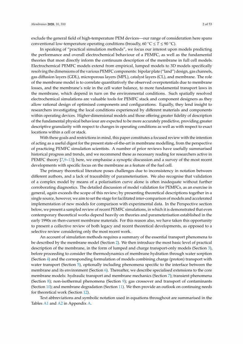
The most well-known example of a PFSA is Nafion, originally developed in the 1960s by DuPont,and now a brand owned by Chemours (Wilmington, DE, USA) [14,15]. Other PFSA materials havebeen widely used in recent years, with the primary differences being the length and chemistry of thechain linking the backbone and acid groups [16]; these include Aquivion [17,18] (originally developedby Dow as Hyflon and now Solvay) and 3M materials [19,20]. Historically, membranes were madesolely of thick extruded sheets of pure proton-conductive polymer; more recently, however, compositemembranes with features such as non-conducting polymer reinforcements (e.g., GORE-SELECTmaterials [21,22]) and radical scavengers [23] (e.g., Nafion XL [24]) have become more common.Figure 1 summarises some of the key developments in membrane technology. While contemporarystate-of-the-art commercial membranes bear little resemblance to their 1960s progenitors, either inform or performance, the underlying chemistry and physics remain largely the same.

Membranes 2020, 10, x FOR PEER REVIEW 3 of 55

2. Proton‐Exchange Membrane: Role and Essential Transport Phenomena

2.1. Role of the Membrane

The purpose of the membrane in a PEMFC is to act as a barrier to gas transport, thereby

preventing direct mixing of H2 and O2, and preventing electron conduction between the anode and

cathode electrodes while acting as an ionic conductor via mobility of protons (H+). The main active

component of PEMFC membranes is the proton‐conductive polymer (ionomer) phase. Most

commonly, the proton‐conductive phase in PEMFCs is a PFSA. These polymers have a perfluorinated

hydrophobic backbone connected to hydrophilic sulfonic acid groups that act as strong acids with

very labile dissociation of protons. In the presence of water, mobile proton‐carrying species (such as

hydronium, H3O+) form, and the ionic conductivity of the membrane is increased significantly.

Membrane hydration is essential for a practically useful proton conductivity to be obtained, so it is

common for models to account for the variability of membrane properties with water content, and to

describe water transport concurrently with proton transport.

The most well‐known example of a PFSA is Nafion, originally developed in the 1960s by DuPont,

and now a brand owned by Chemours (Wilmington, DE, USA) [14,15]. Other PFSA materials have

been widely used in recent years, with the primary differences being the length and chemistry of the

chain linking the backbone and acid groups [16]; these include Aquivion [17,18] (originally developed

by Dow as Hyflon and now Solvay) and 3M materials [19,20]. Historically, membranes were made

solely of thick extruded sheets of pure proton‐conductive polymer; more recently, however,

composite membranes with features such as non‐conducting polymer reinforcements (e.g., GORE‐

SELECT materials [21,22]) and radical scavengers [23] (e.g., Nafion XL [24]) have become more

common. Figure 1 summarises some of the key developments in membrane technology. While

contemporary state‐of‐the‐art commercial membranes bear little resemblance to their 1960s

progenitors, either in form or performance, the underlying chemistry and physics remain largely the

same.

Figure 1. Schematic highlighting the key innovations in polymer electrolyte membrane fuel cell

(PEMFC) membranes.

In the PEMFC modelling literature, the significant majority of works address membrane

materials in the Nafion family, but other PFSA‐based materials, including reinforced membranes, can

be treated through similar theoretical approaches, provided experimental data are available. We

highlight that it is likely to be insufficient to, for instance, use historical data from experiments on

Figure 1. Schematic highlighting the key innovations in polymer electrolyte membrane fuel cell(PEMFC) membranes.

In the PEMFC modelling literature, the significant majority of works address membrane materialsin the Nafion family, but other PFSA-based materials, including reinforced membranes, can be treatedthrough similar theoretical approaches, provided experimental data are available. We highlight that it is

Membranes 2020, 10, 310 4 of 53

likely to be insufficient to, for instance, use historical data from experiments on Nafion 115 membranesin models of very thin, reinforced membranes using a different PFSA. Besides one exception in the recentChinese-language literature [25], we encountered in the literature no instances of models explicitlyaccounting for the altered properties of thin composite materials used in state-of-the-art devices.

Fundamental research has also considered alternative membrane chemistries: for example,those made with non-fluorinated hydrocarbons [15], with multiple acidic head groups [26] or bythe incorporation of new monomers into the backbone [27]. Again, it is likely that such materialscan be treated through similar approaches to those developed for Nafion and discussed in this text,provided sufficient experimental data are available. The hydroxide-conducting membranes used inanion exchange membrane fuel cells feature significantly different transport mechanisms [28] and soany adaptation of the models described here to these materials must be made with great caution.

Similar PFSA-based materials to those used in PEMFCs are also used for the membrane in polymerelectrolyte membrane water electrolyser (PEMWE) applications, and in alcohol-fuelled proton-exchangefuel cells (direct methanol and direct ethanol fuel cells, DMFC/DEFC). In these devices, one or bothfaces of the PEM is in contact with liquid water, altering the environmental equilibration of themembrane material compared to the PEMFC case, where both faces of the membrane meet a gas phase(notwithstanding condensation of liquid water in the CLs), and either face of the membrane may bepartially humidified depending on operating conditions. We shall draw attention to the applications ofthe theories reported herein to PEMWE and DMFC/DEFC simulation, selectively and as appropriate.

2.2. Membrane Types and Fundamental Material Properties

Essential properties of the dry PEM material are its density ρdry and equivalent weight MEW,where the equivalent weight is the mass of polymer per 1 mol of sulfonic acid groups. It is common toreport the available ion-exchange capacity (IEC) measured by titration (often as milliequivalents/gof the acidic functional group), which in an ideal condition is the inverse of the equivalent weight(IEC = 1/MEW) [29]. IEC can also be measured under specified hydration conditions, in which case itwill generally differ from the maximum available IEC.

Nafion 1100 is a standard material with MEW ≈ 1.100 kg mol−1 and ρdry ≈ 2050 kg m−3 [1,30].Both the Nafion 11x and Nafion 21x series have MEW close to this value, with x denoting the thicknessof the manufactured membrane in thousands of an inch (10−3 in, “mil”). We note one recent model [31]giving the dry density as 1970 kg m−3, which is equivalent to the basis weight at 5% water content(50% relative humidity, T = 23 C) given on the Nafion 115 data sheet [32]. In this context it is importantto recognise that the basis weight and dry density are not equivalent concepts—there will exist adiscrepancy depending on the degree of swelling with water uptake (see also Section 7.2, “MembraneExpansion and Mechanical Constraint”, below). Of course, the ideally dry condition is not encounteredin the PEMFC context, and so densities of the hydrated membrane have more practical relevance.The role of water sorption on density is discussed further below (Section 4, “Sorption of Water”).

The concentration of sulfonic acid groups cf in the dry membrane (or, as an inverse, the molarvolume of the dry membrane Vp) is defined as:

cf = V−1p ≡

ρdry

MEW(1)

From the above standard values, cf ≈ 1850 mol m−3, Vp≈ 5.35 × 10−4 m3 mol−1. As a caution,the significant paper on water management by Berg et al. [33] gives cf = 1200 mol m−3 which seemsto be erroneous for Nafion 1100 if measured against the dry density. Even at high water content,which will lower overall density according to (10) below, this value seems too low.

Membranes 2020, 10, 310 5 of 53

2.3. Essential Transport Phenomena in the Membrane

Membrane transport phenomena must be described in a PEMFC model to account for the balanceacross the membrane of the observable quantities of interest (shown schematically in Figure 2) [13].Spatial variation in these quantities may be of interest: both through the plane of the membrane fromanode to cathode, and also in the plane of the membrane, in the case of 2D/3D models that capturespatial variations in the electrode plane due to flow channel design.

Membranes 2020, 10, x FOR PEER REVIEW 5 of 55

2.3. Essential Transport Phenomena in the Membrane

Membrane transport phenomena must be described in a PEMFC model to account for the

balance across the membrane of the observable quantities of interest (shown schematically in Figure 2)

[13]. Spatial variation in these quantities may be of interest: both through the plane of the membrane

from anode to cathode, and also in the plane of the membrane, in the case of 2D/3D models that

capture spatial variations in the electrode plane due to flow channel design.

Figure 2. Schematic of different transport phenomena that can be considered in membrane models.

For an electrochemical device, the most common lumped quantity of interest is the

electrochemical voltage, with the loss of cell voltage due to the membrane corresponding primarily

to resistance to the transport of charge. Since charge is transported in the membrane in the form of

protons (or, proton‐carrying species) it is accompanied by electroosmotic flow of water; thus it is

normally necessary for transport of the following conserved properties to be considered:

charge;

proton mass;

water mass.

In the PEMFC context, it is, therefore, normally considered essential to define transport relations for:

proton flux (current density);

water flux.

Section 3 below will consider simpler models where the water transport is considered ideal, so

that the membrane is uniformly hydrated and a charge transport‐only model can be used. Sections 4–5

will then consider the quantitative theory of water uptake and describe various models coupling

current density to water flux.

If required, the model may be extended by the consideration of other transport phenomena:

momentum (flow/mechanical stress, discussed in Section 7);

heat (discussed in Section 9);

dilute dissolved gas mass, to account for gas crossover (discussed in Section 10.1);

Figure 2. Schematic of different transport phenomena that can be considered in membrane models.

For an electrochemical device, the most common lumped quantity of interest is the electrochemicalvoltage, with the loss of cell voltage due to the membrane corresponding primarily to resistanceto the transport of charge. Since charge is transported in the membrane in the form of protons(or, proton-carrying species) it is accompanied by electroosmotic flow of water; thus it is normallynecessary for transport of the following conserved properties to be considered:

• charge;• proton mass;• water mass.

In the PEMFC context, it is, therefore, normally considered essential to define transport relations for:

• proton flux (current density);• water flux.

Section 3 below will consider simpler models where the water transport is considered ideal,so that the membrane is uniformly hydrated and a charge transport-only model can be used. Sections 4and 5 will then consider the quantitative theory of water uptake and describe various models couplingcurrent density to water flux.

If required, the model may be extended by the consideration of other transport phenomena:

Membranes 2020, 10, 310 6 of 53

• momentum (flow/mechanical stress, discussed in Section 7);• heat (discussed in Section 9);• dilute dissolved gas mass, to account for gas crossover (discussed in Section 10.1);• dissolved ion mass (other than protons, discussed in Section 10.2).

3. Charge Transport-Only Membrane Models

3.1. Zero-Dimensional (0D, Lumped) Resistance Models

The simplest level of description of the electrochemical performance of a PEMFC is an empiricalfit to the electrochemical performance as evidenced by a measured polarisation curve, without anyphysical resolution of the underlying phenomena. Ignoring transport phenomena, a simple fit resolvingthe kinetic and ohmic regions of the polarisation curve (cell voltage Ecell as a function of cell currentdensity icell) is [34]:

Ecell = EOCV −Acat log10

(icell

iref

)−RΩicell (2)

The parameters in this fit are the open circuit voltage EOCV, Tafel slope Acat, reference currentdensity iref, and ohmic series resistance RΩ (Ω·m2). These parameters are determined empirically fromthe polarisation curve data. RΩ is traditionally attributed primarily to the finite proton conductivity ofthe membrane (κ). Thus, for a membrane of thickness Lmem:

RΩ ≈Lmem

κ(3)

For the thinnest membranes this approximation is less reliable, since the contributionsfrom proton transport in the CL and from electrical contact resistances in the cell may becomeproportionally significant.

3.2. Constant Hydration Models

In uncontaminated operating conditions for a PEMFC, there are no dissolved ions in the membraneother than protons: hence, only protons contribute to mobile charge in the membrane, with thecounter-ions present as the static sulfonate groups. Under these conditions, charge transport andproton mass transport are equivalent phenomena—neither one may take place without the other,and so the parameterisation of the transport of the two properties is inextricable. The current density iand molar flux of protons N+ differ only by means of a scaling by the Faraday constant F:

iF= N+ (4)

Although water balance is most often included, if a constant hydration condition is assumedthen a charge transport-only transport theory results [35,36]. The simplest conductivity model is anOhm’s law model of the current density (5) relating current density to proton conductivity (κ) andmembrane-phase electrolyte potential (ϕ). This can then be combined with a statement of conservationof current in the bulk membrane, (6).

i = −κ∇φ (5)

∇ · i = 0 (6)

Within a volume-averaged continuum model [37] of the CL, an effective conductivity may beused according to the volume fraction and connectivity of the ionomer within the CL composite [8,38];also, the electrolyte current balance in the volume-averaged CL will have a source term correspondingto the faradaic current density (and, in principle, capacitive current density) and the correspondingsource/sink of protons to the ionomer.

Membranes 2020, 10, 310 7 of 53

4. Sorption of Water

In a humid or wet environment, the membrane material takes up water through sorption.The water content λ of the polymer is defined as the ratio of moles of sorbed H2O (nH2O) to moles ofsulfonic acid groups (nSO3 ), within a defined reference volume of membrane (V) [1]:

λ =nH2O

nSO3

(7)

The water content may equivalently be written in terms of a total mass of water (mw) taken up inthe same reference volume:

λ =mw

MwcfV(8)

where the molar mass of water Mw = 0.018 kg mol−1.By rearranging (7) and (8), the volume fraction of water in the hydrated PEM (φw) is given:

φw =λ

λ+Vp

Vw

(9)

where Vw is the molar volume of sorbed water ≈ 1.8 × 10−5 m3 mol−1 at 25 C (corresponding to adensity of sorbed water ρw ≈ 1000 kg m−3). The total density of hydrated polymer (ρ) approximatelyobeys a linear relation [1]:

ρ = ρdry(1−φw) + ρwφw (10)

From (9),

ρ =MEW + Mwλ

c−1f + λVw

(11)

We define a hygroscopic swelling coefficient βw to account for membrane volume change underwater uptake:

βw ≡V

Vdry(12)

cw =cf

βwλ (13)

Springer et al. proposed the following linear correlation for βw [39]:

βw ≈ 1 + 0.0126λ (14)

4.1. Sorption Isotherms

A sorption isotherm relates the equilibrium water content λeq to the activity of water aw in themembrane phase:

λeq = λeq(aw) (15)

To reach equilibrium, water may be sorbed from or desorbed to an adjacent phase, which mightbe either a gas phase containing water vapour at a certain activity, or a liquid phase (aqueous phase).These two cases are referred to as vapour-equilibrated (VE) and liquid-equilibrated (LE) conditions,respectively. It has been widely observed experimentally that the sorbed water uptake to PFSAionomers is different between VE exposure to saturated water vapour and LE exposure to pureliquid water. Since both saturated water vapour and pure liquid water both have an activity aw = 1,this result is thermodynamically unexpected and is often called “Schröder’s paradox” [40]: it isgenerally explained according to the presence of liquid water promoting an otherwise restricted phasetransition of the ionomer that either eliminates the vapour–liquid interface near the membrane surface,or alters the energetics of the ionomer matrix–liquid contact [41–44].

Membranes 2020, 10, 310 8 of 53

Some experimental studies (notably Jeck et al. [45]) report an absence of Schröder’s paradox,but also suggest VE water contents that are higher than presented in other studies and closer to atypical LE value, possibly implicating the presence of a thin water film. The capability of thin waterfilms to maintain bulk LE conditions in membranes with one VE face has also been suggested, basedon X-ray tomography evidence [46].

The presence of VE or LE conditions also influences the interfacial resistance to the recovery ofthe sorption equilibrium, which will be discussed further below (Section 6) in the context of interfacialphenomena. It is relevant to note that whereas a PEMFC may be operated under VE conditions atboth electrodes, PEMWE operation is likely to be LE at both electrodes, except possibly at high currentdensity where gas production rate may reduce the extent of wetting. Likewise, liquid-fed DMFCs andsimilar devices would typically be liquid-equilibrated at the anode face of the membrane in contactwith aqueous solution; in this case, however, the activity of water in the liquid phase is not necessarilyequal to unity, due to the presence of the concentrated alcohol component.

Under VE conditions, the activity of water in the membrane (aw) can be specified as equal to theactivity of water vapour in the equilibrating gas phase (aw,vap):

aw = aw,vap (equilibrium) (16)

The activity of water in the vapour phase can in turn be approximated as a function of the partialpressure of water (pw,vap) and the saturated partial pressure of water (vapour pressure, psat) as afunction of temperature (T):

aw,vap ≈pw,vap

psat(T)(17)

Equation (17) neglects fugacity corrections, which is normally suitable for PEMFC operating conditionsat absolute pressures of a few bar.

The vapour pressure of water used in (17) is conventionally expressed as an empirical function oftemperature [47]. Springer et al. used curve fitting on tabulated values for the vapour pressure to givethe following standard expression, used also in recent PEMFC models (coefficient data tabulated inTable 1) [39,48]:

log10

(psat

p0

)= a0 + a1(T − T0) + a2(T − T0)

2 + a3(T − T0)3 (18)

Table 1. Parameterisation of the Springer et al. water vapour pressure fit, with p0 = 1 atm andT0 = 0 C [39].

Coefficient Value

a0 −2.1794a1 +0.02953 K−1

a2 −9.1837 × 10−5 K−2

a3 +1.4454 × 10−7 K−3

Gurau et al. reported an alternative fit given by the American Society of Heating, Refrigeratingand Air-Conditioning Engineers (ASHRAE) (coefficient data tabulated in Table 2) [49]:

ln( psat

1Pa

)=

b−1

(T/1K)+ b0 + b1(T/1K) + b2(T/1K)2 + b3(T/1K)3 + be ln(T/1K) (19)

Membranes 2020, 10, 310 9 of 53

Table 2. Parameterisation of the American Society of Heating, Refrigerating and Air-ConditioningEngineers (ASHRAE) water vapour pressure fit reported by Gurau et al. [49].

Coefficient Value

b−1 −5.8002206 × 103

b0 1.3914993b1 −0.048640239b2 4.1764768 × 10−5

b3 1.4452093 × 10−8

be 6.5459673

The specification of the sorbed water activity under LE conditions typically depends on extendingthe range of values aw to aw > 1, according to a saturation-dependent definition of activity in thepresence of liquid water. Simultaneously, the sorption isotherm (15) is extended to the correspondingvalues of aw. For instance, Springer et al. defined for the purposes of the sorption equilibrium that [39]:

aw ≡xwppsat

(20)

where the mole fraction of water xw includes both liquid- and gas-phase water. It should be noted thatthis definition is dependent on the use of a pseudo-two phase description of material transport in theGDL and CL, whereby liquid water is treated a gas-phase species with no independent momentumconservation. More detailed two-phase models, in which liquid water saturation in the porous diffusionmedia is described through an additional variable with a corresponding transport equation [10,50],may require an alternative specification of the LE sorption condition.

4.2. Empirical Sorption Models for Nafion 1100

A number of empirical sorption isotherms have been established experimentally based onmeasurements on Nafion 1100 [39,51–54]. All sorption isotherms reported in this subsection wereparameterised for this material and, therefore, applications to other related materials—even in theNafion family—should be undertaken with caution. A selection of the isotherms reported in thissubsection are summarised in Figure 3.

The most commonly used sorption isotherm is an empirical polynomial relation due toSpringer et al. [39]:

λeq = 0.043 + 17.81aw − 39.85a2w + 36.0a3

w, 0 ≤ aw ≤ 1λeq = 14 + 1.4(aw − 1), 1 ≤ aw ≤ 3

(21)

The definition for supersaturated conditions (aw > 1) aims to account for Schröder’s paradoxthrough the definition (20) given above. The polynomial relation is specific to measurements at 30 C,although the definition for aw > 1 derives from liquid-equilibration data at 80 C.

Kusoglu and Weber offered an alternative polynomial fit for VE conditions at 30 C by averaginga wide range of experimental data (from different authors) [1]:

λeq = 0.05 + 20.45aw − 42.8a2w + 36.0a3

w, 0 ≤ aw ≤ 1 (22)

In spite of a variety of experimental investigations, there exist no definitive data for the temperaturedependence of the sorption equilibrium at the higher temperatures more typical of PEMFC operation.Most data, however, suggest a relatively weak temperature dependence up to T = 90 C: for thisreason, it is common in the literature to encounter (21) being used at a typical PEMFC operatingtemperature also.

Membranes 2020, 10, 310 10 of 53Membranes 2020, 10, x FOR PEER REVIEW 10 of 55

Figure 3. Summary of measured sorption isotherms for Nafion 1100 in the vapour‐equilibrated range

of aw.

In spite of a variety of experimental investigations, there exist no definitive data for the

temperature dependence of the sorption equilibrium at the higher temperatures more typical of

PEMFC operation. Most data, however, suggest a relatively weak temperature dependence up to T =

90 °C: for this reason, it is common in the literature to encounter (21) being used at a typical PEMFC

operating temperature also.

Hinatsu et al. measured the following sorption isotherm at 80 °C [55]:

2 3eq w w w w0.3 10.8 16.0 14.1 1, 0λ a a a a (23)

while Pasaogullari et al. [56] presented a fit to data from Zawodzinski et al. [53] under VE conditions

at 80 °C as:

2 3eq w w w w1.4089 11.263 18.7 168 16.209 , 0λ aa a a (24)

Kulikovsky extended the above expression to a super‐saturated or LE condition [57]:

w

eq w w w

0.890.3 6 1 tanh 0.5 3.9 1 tanh

0.23

aλ a a a (25)

As shown in Figure 3, the Pasaogullari and Kulikovsky isotherms at higher temperature predict

overall lower water contents than the Springer isotherm at ambient temperature, especially close to

aw = 1.

Meier and Eigenberger proposed a 25 °C isotherm (expressing activity as a function of water

content) which is compatible with LE conditions but without exceeding aw = 1 [58]:

2w eq eq

w eq eqeq

5

0.01355 ,

2.751.435

0

0.0

0. 3 2.5

0.022 ,13 ln 2.

a λ λ λ

λ λλ

a λ (26)

Figure 3. Summary of measured sorption isotherms for Nafion 1100 in the vapour-equilibrated rangeof aw.

Hinatsu et al. measured the following sorption isotherm at 80 C [55]:

λeq = 0.3 + 10.8aw − 16.0a2w + 14.1a3

w, 0 ≤ aw ≤ 1 (23)

while Pasaogullari et al. [56] presented a fit to data from Zawodzinski et al. [53] under VE conditions at80 C as:

λeq = 1.4089 + 11.263aw − 18.768a2w + 16.209a3

w, 0 ≤ aw ≤ 1 (24)

Kulikovsky extended the above expression to a super-saturated or LE condition [57]:

λeq = 0.3 + 6aw(1− tanh(aw − 0.5)) + 3.9√

aw

(1 + tanh

(aw − 0.890.23

))(25)

As shown in Figure 3, the Pasaogullari and Kulikovsky isotherms at higher temperature predictoverall lower water contents than the Springer isotherm at ambient temperature, especially close toaw = 1.

Meier and Eigenberger proposed a 25 C isotherm (expressing activity as a function of watercontent) which is compatible with LE conditions but without exceeding aw = 1 [58]:

aw = 0.01355λeq + 0.03λ2eq, λ ≤ 2.5

aw = 1.435 + 0.0022λeq −2.75λeq− 0.13 lnλeq, λ > 2.5 (26)

Similarly, Karpenko-Jereb et al. originated an alternative empirical sorption isotherm with asmoothed jump at 0.97 ≤ aw ≤ 1 to represent Schröder’s paradox, wherein the VE sorption isothermshows no temperature dependence, but a temperature dependence is incorporated in the LE part [59]:

λeq,V = 1.55 + 13.71aw − 24.37a2w + 21.87a3

wλeq,L = 41.83 T

T0− 28.31

λeq = λeq,V, aw < 0.97λeq = λeq,V +

(λeq,L − λeq,V

)(aw−0.97

0.03

), 0.97 ≤ aw ≤ 1

(27)

Membranes 2020, 10, 310 11 of 53

with T0 = 303.15 K.Futerko and Hsing gave the temperature dependence of the LE water content with T0 = 273 K

as [60]:λeq,L = 10 + 0.0184(T − T0) − 9.9× 10−4(T − T0)

2 (28)

4.3. Detailed Sorption Models

A number of authors have attempted to construct sorption models based on more fundamentalproperties of the PEM, rather than from a purely empirical basis. Again, all parameterisation in thissubsection is reported for Nafion 1100.

Futerko and Hsing applied a Flory–Huggins model to express the activity of the membrane underVE conditions as [60]:

aw = (1−φm) exp((

1− Vw

Vp

)φm + χφ2

m

)φm =

Vp+Vw

Vp+λVw

(29)

where the Flory parameter χ = 1.936 − (2.18 kJ mol−1)/RT and φm is the effective membranevolume fraction.

Thampan et al. suggested following the Brunauer–Emmett–Teller (BET) adsorption isotherm,expressed as follows [30]:

λeq = λeq,Thampan = λmono

(K1

aw1−aw

)(1− (nw,sat + 1)anw,sat

w + nw,sata1+nw,satw

)1 + (K1 − 1)aw −K1a1+nw,sat

w

(30)

Here, λmono is the water content corresponding to an effective ‘monolayer coverage’ withinthe polymer scaffold of the membrane, which was assumed = 1.8. The other parameters are fittingcoefficients to experimental data [52,61] with values given as K1 = 150 and nw,sat = 13.5. The BETisotherm predicts a saturated VE water content in terms of its parameters as [62]:

λsat = limaw→1

λeq,Thampan = λmonoKln2

w,sat

1 + Klnw,sat(31)

Klika et al. advocated the Guggenheim–Anderson–de Boer (GAB) isotherm, which extends theBET isotherm with an energy difference between the bulk and multilayer sorbed states of the waterrepresented by the quantity kG, replacing nw,sat in (30). Their equation is [63]:

λeq = λmonoK1kGaw

(1− kGaw)(1 + (K1 − 1)kGaw)(32)

with empirical parameters fit to experimental data [39,45] as λmono = 1.93, K1 = 44.3 and kG = 0.9.Choi and Datta argued that Schröder’s paradox can be explained by the restricted morphology

of the vapour–liquid interface within a pore, which is resolved by liquid equilibration [41]. Theirwork derived a rather complicated expression for the sorption isotherm that extends the Thampanisotherm (Equation (30)) for both vapour- and liquid-equilibrated modes, considering bound wateras a separate Langmuirian contribution to the isotherm, with a BET model accounting for additionalbound water uptake beyond a monolayer, and a Flory–Huggins isotherm for free water. The resulting,rather unwieldy implicit equations relate to (30) as:

(1− λeq,Thampan

)aw exp

VwRT

κsorpλeq,L

λeq,L+VpVw

− 1

λeq,L = 1

(1− λeq,Thampan

)aw exp

VwRT

κsorpλeq,V

λeq,V+VpVw

− aporeγw cosθc

(1 +

Vp

Vwλeq,V

)− 1

λeq,V = 1

(33)

Membranes 2020, 10, 310 12 of 53

The fitted parameters were as above, except setting K1 = 100 and nw,sat = 5. Additional parametersare defined in Table A2 in Appendix A, and given as κsorp = 183 atm, apore = 2.1 × 108 m−1,γw = 0.0721 N m−1, θc = 98.

In the context of a DMFC, Meyers and Newman developed an isotherm based on fundamentalenergetics of the PEM [64]. Like the model of Thampan et al. [30], this model combines anacid-base equilibrium for dissociation of sulfonic acid groups in the membrane with a requirement ofelectroneutrality. The resulting simultaneous equations that define the isotherm are (coefficient datatabulated in Table 3) [64]:

aw = K2(λeq − λ+

)exp(φ2λ+) exp

(φ3λeq

)λ+ exp(φ1λ+) exp

(φ2λeq

)= K1(1− λ+)

(λeq − λ+

) (34)

where λ+ is the ratio of moles of hydronium ions to moles of sulfonic acid sites and must be solved forself-consistently. The ϕn coefficients are defined as:

φ1 = 2MEW

(E00 − 2E++ − 2E+0)

φ2 = 2MEW

(E+0 − 2E00)

φ3 = 2MEW

E00

(35)

Table 3. Parameterisation of the Meyers–Newman sorption model for Nafion 1100 at T = 30 C [52,61].

Coefficient Value

K1 100K2 0.217E00 −0.0417 kg mol−1

E+0 −0.052 kg mol−1

E++ −3.7216 kg mol−1

The Meyers–Newman isotherm was applied by Weber and Newman using the above parameters,subject to a further empirical modification to account for inaccuracies of the model at low wateruptake [65]:

λ = βλeq(1 + exp

(λeq,crit − λeq

))(36)

with the scaling coefficient β = 1 (included for generality, see Section 4.4, “Sorption within the CatalystLayer” below) and λeq,crit = 0.3. Subsequently, the influence of temperature on this sorption isothermwas accounted for by treating all inputs as temperature-independent except K2, which varies as [66]:

K2 = 0.217 exp(

∆Hsorp

R

(1

T0−

1T

))(37)

with T0 = 303.15 K and the enthalpy change of sorption ∆Hsorp = +1 kJ mol−1.Murahashi et al. [67] and Eikerling and Berg [44] and have both argued for the influence of size

distribution of pores upon the sorption isotherm. Smaller pores may retain water due to the pressuredrop of the liquid–vapour interface, even when larger pores become dehydrated [67]. Eikerling andBerg argued that pores with a range of surface charge densities can wet progressively due to morehighly charged pores taking up water more slowly, but attaining larger limiting wetted radii [68]. Sincethe Eikerling–Berg description makes a number of highly specific assumptions about the geometryand governing phenomena of the matrix-liquid-vapour system, it could be viewed as didactic ratherthan being directly usable for quantitative modelling of membrane sorption in the PEMFC context.

Membranes 2020, 10, 310 13 of 53

4.4. Sorption within the Catalyst Layer

It has been established experimentally that membrane material within the composite structure ofthe catalyst layer takes up proportionally less water by sorption than in the bulk membrane [69,70].This has been attributed to the altered internal morphology of Nafion ionomer when present asa <60 nm film. Recent analysis has indicated that a lamellar structure forms for particularly thinfilms, and that total water uptake varies non-monotonically with film thickness [71]. This work hasalso emphasised that for thin films, homogenisation of material properties is typically unreasonable,and interfacial phenomena may dominate.

It has been proposed that the CL water uptake could be described empirically by setting K2 = 0.231,β = 0.342 (all other parameters identical) in the Meyers–Weber–Newman isotherm (36) [70]. This workalso assumed a constant apparent proton conductivity κeff = 10−4 S m−1 in the CL. Incorporation intoa full PEMFC model was reported to give improved accuracy in the prediction of performance lossdue to anode dehydration, under low relative humidity operating conditions. From a thermodynamicpoint-of-view, it is necessary to recognise that altering the isotherm in the CL specifically implies aphase transition for water between the CL ionomer and the bulk membrane, at constant activity. If noresistance is incorporated for this transfer, reduced water uptake in the CL remains compatible withnormal water content and water transfer fluxes in the bulk membrane.

Additionally, studies have suggested that sorbed water uptake of the CL depends upon Ptloading [69], choice of carbon support [38,72], and the solvent used in CL preparation [73]. Using thePt/C-phase effective electronic conductivity as a probe, Morris et al. showed that sorption/desorptionin the CL appeared to be free from hysteresis [74].

Mashio et al. provided a comprehensive model for CL water uptake in which sorption to themembrane was incorporated by means of a Langmuir isotherm [72]:

λ = λsatKmemawpsat

1 + Kmemawpsat(38)

with equilibrium constant Kmem = 3.3 × 10−4 Pa−1; this work stresses the role of water adsorption on avariety of materials within the CL, in terms of overall water uptake of this region.

Since the CL has a high volumetric surface area of contact between vapour- or liquid-phase waterand the membrane material, the local sorption properties in this region may significantly influencethe overall water balance of the membrane. Kosakian et al. have recently presented a dedicated CLisotherm as follows [75]:

λeq =(6.932aw − 14.53a2

w + 11.82a3w

)exp

(θsorp

(1

T0−

1T

)), 0 ≤ aw ≤ 1

λeq = 22, aw > 1(39)

with θsorp = 2509 K, T0 = 303.15 K. It should be noted that this specification gives a large discontinuityat the transition to liquid equilibration at aw = 1; this is not depicted in Figure 3 which focuses onVE conditions.

5. Coupled Proton-Water Transport

As introduced through the discussion above in Section 2.3 (“Essential Transport Phenomena inthe Membrane”), current flow by proton flux through the membrane is always accompanied by watertransport due to electroosmotic drag. Therefore, the majority of practical membrane models usedin PEMFC simulation are coupled models incorporating both proton and water transport. In thissection, we will introduce some essential considerations surrounding the coupling of the two transportprocesses, and then consider three principal approaches to this coupling and their parameterisation.

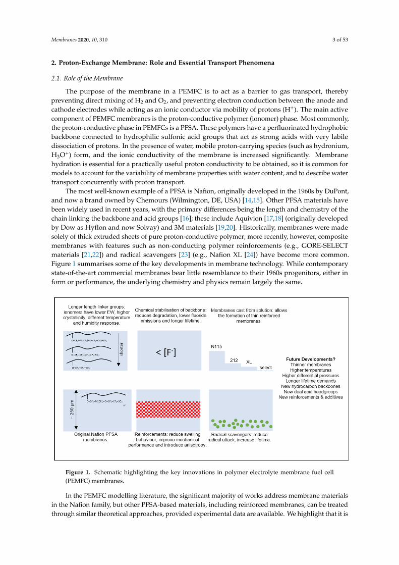
First, we will discuss the membrane model originated in the seminal early PEMFC simulation workby Springer, Zawodzinski and Gottesfeld [39] (hereafter “Springer model” for brevity). This widely usedmodel accounts for electroosmotic drag and water diffusion in an essentially empirical manner. Second,

Membranes 2020, 10, 310 14 of 53

the Weber–Newman model [65] will be considered; this model is rooted in a more formal derivationfrom non-equilibrium thermodynamics of the membrane phase, but remains empirically parameterised.Lastly, the binary friction model developed by Djilali and co-workers will be discussed [76–78].

Weber and Newman have advocated the interpretation of the hydrated membrane as a systemwith three chemical components: water, protons, and fixed membrane structure [65]. Therefore, thereexist no more than three independent transport properties associated with the binary interactions ofthe three components. If bulk momentum transfer through the membrane is considered, mechanicalresistance (friction) may account for a fourth transport property. The three most experimentallyaccessible choices for the definition of the three independent transport properties, following theWeber–Newman scheme, are [65]:

• proton conductivity κ—the ratio of current density to electrolyte potential gradient for uniformwater content;

• electroosmotic drag coefficient ξ—the ratio of water flux to current density for uniformwater content;

• water diffusivity Dw—the ratio of water flux to water concentration gradient for zerocurrent density.

Parameterisation for each of these intrinsic properties (proton conductivity, water diffusivity,electroosmotic drag coefficient) will be summarised in Section 5.4, Section 5.5, Section 5.6. The rigorousmeasurement of these properties for Nafion 1100 was initiated in the early 1990s in a series of works byZawodzinski et al. [52,53,79,80] and Fuller and Newman [81].

Since the fixed membrane structure is considered rigid (there is no mechanical translation of themembrane), the Weber–Newman scheme considers only water and proton fluxes, and each of thesefluxes has a conjugate thermodynamic variable whose gradient indicates the direction and magnitudeof the flux. Formal treatments define [65,82]:

• membrane-phase electrolyte potential ϕ as the thermodynamic variable conjugate to the drivingforce for current flow, under uniform hydration;

• chemical potential of water µw (expressed as required in terms of the local water content λ) as thethermodynamic variable conjugate to the driving force for water flux, at zero proton current.

From a thermodynamic standpoint, the inclusion of pressure as a local variable, in additionto electrolyte potential and water content, is almost certainly an overdetermination of the systemexcept for the liquid-equilibrated case; it has not found general support [65,78]. Exceptions in theliquid-equilibrated case, where free water channels may be present, will be discussed further inSection 5.7 below.

5.1. Springer Membrane Model

Springer et al. defined the flux of water through the membrane (Nw) phenomenologically as thesum of a Fickian diffusion term in water concentration cw, and an electroosmotic drag term [9,39]:

Nw = −Dw∇cw + ξiF

(40)

This is compatible with the transport property definitions given above; non-linear transportbehaviour is implied if the coefficients Dw and ξ are themselves functions of water content. Using (14):

Nw = −Dwcf∇

(λβw

)+ ξ

iF

(41)

Membranes 2020, 10, 310 15 of 53

On the basis that βw is a function of water content only, the Springer water flux formula canbe further abbreviated. Springer et al. expressed the water gradient ∇dry with respect to a fixed,dry-membrane coordinate which is undeformed by swelling under water uptake [39]:

Nw = −Dλcf∇dryλ+ ξiF

(42)

where the apparent diffusion coefficient with respect to water content (Dλ) is given:

Dλ =Dw

β2w

(1−

λβw

∂βw

∂λ

)(43)

While the original Springer et al. work considered membrane expansion under swelling,subsequent works have assumed that the compressed membrane has no thickness variation [83];the role of compression is discussed further below in Section 7.2. Thus one can write simply:

Nw = −Dλcf∇λ+ ξiF

(44)

Typically, this diffusivity Dλ is parameterised directly from experimental data, as discussedfurther in Section 5.5 below. Within the membrane, conservation of water mass requires that, understeady-state conditions:

∇ ·Nw = 0 (45)

The widely used Springer model describes coupled proton-water transport in PEMFC membranesby combining Equations (44) and (45) with the Ohm’s law expressions (5) and (6). The interactionof the two transport processes is expressed by the electroosmotic drag term in (44) and the watercontent-dependence of the proton conductivity in (5).

5.2. Weber–Newman Membrane Model

The Weber–Newman model is an alternative to the Springer model that seeks to consider thenon-equilibrium thermodynamics of the coupled proton and water transport processes in a moreformal and consistent manner [65]. Moreover, the empirically determined transport properties areassumed to have different definitions in the VE and LE regimes.

The substantive difference between the transport equations used for the Weber–Newman modeland the Springer model is the presence of a cross-term contribution to the current density expression dueto water streaming current, which is non-zero wherever the water chemical potential is non-uniformthrough the membrane. This phenomenon accounts for the symmetry of the binary proton–waterinteraction: just as electroosmotic drag describes the motion of water molecules due to proton current,so the streaming current describes the motion of protons due to water diffusion. Specifically:

i = −κ∇φ−κξF∇µw (46)

The water flux is then given as, alongside (46) [65]:

Nw,m = −αw,m∇µw,m +ξm

Fi (47)

where the subscript m = V or L and indicates VE or LE conditions.The relation between the intrinsic transport coefficient αw and the apparent Fick’s law diffusion

coefficient Dλ has been expressed differently by various authors [65,83]. A simple interpretation

Membranes 2020, 10, 310 16 of 53

for the VE case has been given by Setzler and Fuller, on the basis that the water content is the onlyparameterising variable for the local state of the hydrated membrane:

−αw,V∇µw = −Dλcf∇λ

= −Dλcf∂λ∂aw

∂aw∂µw∇µw

= −Dλcf∂λ∂aw

awRT∇µw

= −DλcfλRT

∂ lnλ∂ ln aw

∇µw

= −DλcwRT

∂ lnλ∂ ln aw

∇µw

(48)

If the self-diffusion coefficient Dµ is defined as given by Springer et al. [39]:

αw,V ≡ Dµcw

RT(49)

then the two diffusion coefficients are simply related by the Darken factor [83]:

Dλ =∂ ln aw

∂ lnλDµ (50)

However, it should be noted that in their original work, Weber and Newman used instead ofthe definition (49) the following definition based on the Maxwell–Stefan diffusion coefficient for themembrane-water system as a binary system [65]:

αw,V ≡ Dµ,WNcw

RT(1 + λ) (51)

In interpreting the diffusivity data given below in Section 5.5, the inequivalence of (49) and (51)must be borne in mind.

5.3. Binary Friction Model (BFM)

The binary friction model (BFM) is derived beginning from a generalised diffusion equationpresented succinctly in the following form [82]:

Vw

(N+

Nw

)= −

(D11 D12

D21 D22

)( FRT∇φ

∇λ

)(52)

where the generalised diffusion coefficients Dmn are functions of λ,T, thereby accountingfor non-linearity.

In the BFM developed by Fimrite, Carnes, Struchtrup and Djilali [76,77], the mole fraction ofproton carriers is derived using a method originated by Thampan et al. [30] This mole fraction is thenapplied as a dependent variable in a concentrated solution theory; Shah et al. have also applied theThampan method previously to dilute solution theory [84]. The Thampan approach assumes that thereexists an acid-base equilibrium quantifying the degree of dissociation of the sulfonic acid groups in thefixed membrane structure [30]:

SO3H(fixed) + H2OKa,mem SO−3 (fixed) + H3O+ (53)

In this case, the total water content is divided between neutral water and charged hydroniumspecies. Electroneutrality requires that the local concentrations of H3O+ and SO3

− are equal. Lateriterations of the BFM employed the simplifying assumption that sulfonic acid dissociation is complete(strong acid behaviour) [78,82].

In the original BFM, there were five fitted parameters, but no further empirical relations to watercontent [77]. Fimrite et al. thereafter used the term “BFM2” for a specialised binary friction model

Membranes 2020, 10, 310 17 of 53

specific to the PEMFC device context, in the limit of complete sulfonic acid group dissociation [78,82].This model has six parameters, which were fitted to a conductivity vs. water content curve derivedfrom alternating current (AC) impedance measurements. (As an aside, the original derivation of theBFM2 model is complicated by two irregular negative multiples: one in the definition of the potentialdriving force ([82], eqn 3) and then one in the charge of the hydronium ion (set = −1 in [82]). Thesenegatives cancel in the derived equations.) The resulting Weber–Newman transport coefficients arethen expressed in terms of a set of binary diffusivities as [82]:

κ = feffcfF2

RTD+m

λ

D0m + D+0λ

D+0λ+ D+m + D0m(λ− 1)(54)

ξ =D0m(λ− 1)

D0m + D+0λ(55)

Dw = feffD0m

λ

D+0

D+0λ+ D+m + D0m(λ− 1)(56)

The three binary diffusivities are expanded further as functions of temperature and/or watercontent, as:

Dkm = D+0Akλs (57)

D+0 = D+0,ref exp(θdiff

(1

Tref−

1T

))(58)

and the coefficient f eff accounts for the influence of an effective ‘membrane porosity’ by the relation:

feff = (φw(λ) −φw(λmin))q (59)

The more explicit definition of the functional forms of each of the three orthogonally measurabletransport coefficients in terms of the various water-content-independent parameters is suggested as ameans to reduce the degree of empiricism in the model setup (coefficients are tabulated in Table 4).

Table 4. Parameterisation of the binary friction model for Nafion 1100 [78,82].

Coefficient Value

λmin 1.65D+0 6.5 × 10−9 m2 s−1

s 0.83q 1.5

A+ 0.084A0 0.5θdiff 1800 K

Djilali and Sui [85] have argued that the above theory offers improved sensitivity to the variation inmembrane behaviour under conditions of low anode humidification, where the empirical correlationsfrom Springer et al. [39] may be less reliable. Conversely, it is unclear whether the BFM will retainapplicability in the limit of high water content or liquid-equilibration, where hydraulic transportbecomes significant.

5.4. Proton Conductivity as a Function of Water Content

The proton conductivity κ appears in both the Springer model and the Weber–Newman model asan empirical function of water content. Within the Weber–Newman model, proton conductivity isadditionally considered to have a different value under LE conditions. At the atomic scale, protontransport in a PEM is understood to occur due to two possible mechanisms: the vehicle mechanism,in which protons are carried in the form of hydronium ions, H3O+; and the hopping (Grotthuss)

Membranes 2020, 10, 310 18 of 53

mechanism, in which protons are transported by a hydrogen bond-mediated long-range rearrangementof the bonding network between water molecules and hydronium ions, as in bulk liquid water [42].Since membranes at lower hydration do not contain connected liquid regions with extensive hydrogenbonding networks, the Grotthuss mechanism is suppressed and the vehicle mechanism is believedto dominate [1,2]. Activation of the Grotthuss mechanism for higher water content, especially whenliquid-equilibrated, increases the conductivity as water content rises.

Various empirical relations reported in this subsection for proton conductivity of Nafion 1100materials are plotted in Figure 4 (T = 30 C) and Figure 5 (T = 80 C).

Membranes 2020, 10, x FOR PEER REVIEW 19 of 55

Figure 4. Summary of measured proton conductivity for Nafion 1100 in the vapour‐equilibrated range

of λ at room temperature (T = 30 °C).

Figure 4. Summary of measured proton conductivity for Nafion 1100 in the vapour-equilibrated rangeof λ at room temperature (T = 30 C).

Membranes 2020, 10, x FOR PEER REVIEW 20 of 55

Figure 5. Summary of measured proton conductivity for Nafion 1100 in the vapour‐equilibrated range

of λ at typical PEMFC operating temperature (T = 80 °C).

The functional dependence of conductivity with respect to water content has been expressed in

terms of a polynomial relationship, where there exists some minimum water content λ0 required for

proton conductivity, based on a percolation theory in which there is a need to form connected

hydrated channels through which protons can migrate [42,86]. Additionally, an activation energy is

included for non‐isothermal processes.

cond

0

0 0 cond 00

0,

1 1exp ,

n

κ λ λ

κ λ λ θ λ λT T

(60)

For Nafion 1100, the average value for the exponent ncond through a range of studies [1,59] is ≈ 1.5,

but some empirical models have applied other data values, as summarised in Table 5. In particular,

early studies on proton conductivity as a function of water content supported an approximately

linear relation [39,52]. Relations for which θcond is undefined apply only at T = T0.

Table 5. Summary of polynomial proton conductivity relations, with T0 = 303.15 K.

Data Source κ0/S m−1 λ0 θcond/K ncond

Springer [39] 0.5139 0.6344 1268 1

van Bussel–Kulikovsky [57,87] 0.5736 1.253 undefined 1

Weber [65] 0.2646 2 1800 1.5

Wiezell [88], fit to Zawodzinski [52] 0.45 0.222 undefined 1

Meier [58], fit to Zawodzinski [79] 0.491 * 0.543 1190 1

* Original value is 0.46 at T0 = 298.15 K.

The lower activation energy (θcond ≈ 1300 K) was supported by the experimental measurements

by Karpenko‐Jereb et al. [59]. Moreover, this work sets the dependence strictly in terms of volume

fraction rather than water content:

Figure 5. Summary of measured proton conductivity for Nafion 1100 in the vapour-equilibrated rangeof λ at typical PEMFC operating temperature (T = 80 C).

Membranes 2020, 10, 310 19 of 53

The functional dependence of conductivity with respect to water content has been expressed interms of a polynomial relationship, where there exists some minimum water content λ0 required forproton conductivity, based on a percolation theory in which there is a need to form connected hydratedchannels through which protons can migrate [42,86]. Additionally, an activation energy is included fornon-isothermal processes.

κ = 0, λ < λ0

= κ0(λ− λ0)ncond exp

(θcond

(1

T0−

1T

)), λ ≥ λ0

(60)

For Nafion 1100, the average value for the exponent ncond through a range of studies [1,59] is ≈1.5, but some empirical models have applied other data values, as summarised in Table 5. In particular,early studies on proton conductivity as a function of water content supported an approximately linearrelation [39,52]. Relations for which θcond is undefined apply only at T = T0.

Table 5. Summary of polynomial proton conductivity relations, with T0 = 303.15 K.

Data Source κ0/S m−1 λ0 θcond/K ncond

Springer [39] 0.5139 0.6344 1268 1

van Bussel–Kulikovsky [57,87] 0.5736 1.253 undefined 1

Weber [65] 0.2646 2 1800 1.5

Wiezell [88], fit to Zawodzinski [52] 0.45 0.222 undefined 1

Meier [58], fit to Zawodzinski [79] 0.491 * 0.543 1190 1

* Original value is 0.46 at T0 = 298.15 K.

The lower activation energy (θcond ≈ 1300 K) was supported by the experimental measurementsby Karpenko-Jereb et al. [59]. Moreover, this work sets the dependence strictly in terms of volumefraction rather than water content:

κ = 0, φw < φw,0

= κ0,φ(φw −φw,0

)ncond exp(θcond

(1

T0−

1T

)), φw ≥ φw,0

(61)

This gives approximate equivalence to the tabulated values above when the denominator in (13)is assumed to be constant.

Ju et al. applied the Springer data to a GORE-SELECT membrane with a scaling factor 0.5 toaccount for tortuosity due to the reinforcement [89].

Ramousse et al. repeated a higher-order polynomial fit due to Neubrand [90,91]:

κ/Sm−1 =(0.2658λ+ 0.0298λ2 + 0.0013λ3

)exp

(θcond

(1

T0−

1T

))(62)

with a water content-dependent activation energy:

θcond/K = 2640 exp(−0.6λ) + 1183 (63)

Dobson et al. quoted a polynomial expression for Nafion 211 [92]:

κ/Sm−1 =(2.0634 + 1.052λ+ 0.010125λ2

)exp

(θcond

(1

T0−

1T

))(64)

with θcond = 751.4 K.

Membranes 2020, 10, 310 20 of 53

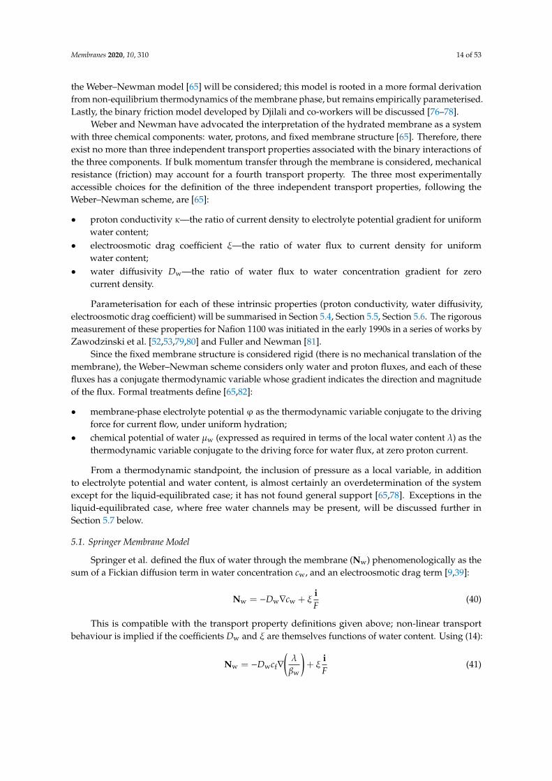
Using the wide data set for proton conductivity compiled by Sone et al. [93], Baschuk and Litabulated third-order polynomial fit data for the water-content dependence of conductivity, at a rangeof temperatures from T = 20 C to T = 70 C [94].

Setzler and Fuller used impedance measurements under varying relative humidity conditions toproduce the following empirical relation for Nafion 212 at 80 C [95]:

κ = κ0 exp(αλ

λλcrit

)(65)

with κ0 = 1.55 S m−1 and αλ = 2.2.Weber and Newman defined the conductivity under LE and VE conditions (indexed as m = L

or m = V below) as depending upon the local volume fraction of water present under the givenequilibration condition, without any specification of how the empirical expressions were derived [65]:

κm/Sm−1 =

10−9 φw,m < φw,crit

κ0(φw,m −φw,crit

) 32 exp

(EA,cond

R

(1

T0−

1T

))φw,crit ≤ φw,m ≤ φw,max

κ0(φw,max −φw,crit

) 32 exp

(EA,cond

R

(1

T0−

1T

))φw,m > φw,max

(66)

with κ0 = 50 S m−1 at T0 = 298.15 K, EA,cond = +15 kJ mol−1, and ϕw,crit = 0.06, ϕw,max = 0.45.Kosakian et al. have presented a specific formulation for proton conductivity in the CL ionomer

(below) [75]. It should be noted that this expression has no stated correlation to porosity or tortuosityproperties of the ionomer in the CL composite, so the absolute magnitude of the conductivity it reportscannot be applied generally to any CL; however, the functional form of the water content-dependencemight be considered more widely applicable.

κ =

3∑i=0

aiωi

exp(

EA,cond

R

(1

T0−

1T

))(67)

ω =

100

((3∑

i=0biλ

i))

0 < λ < 13

100 λ ≥ 13(68)

with EA,cond = +15 kJ mol−1 (polynomial data tabulated in Table 6).

Table 6. Parameterisation of the catalyst layer proton conductivity model given by Kosakian et al.,T = 80 C [75].

i ai bi

0 −0.8 −0.12541 0.075 0.18322 −6.375 × 10−4

−8.65 × 10−3

3 1.93 × 10−5 9.4 × 10−5

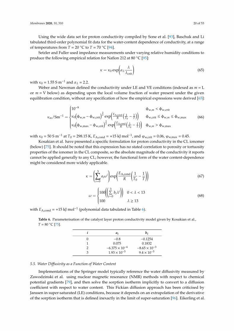
5.5. Water Diffusivity as a Function of Water Content

Implementations of the Springer model typically reference the water diffusivity measured byZawodzinski et al. using nuclear magnetic resonance (NMR) methods with respect to chemicalpotential gradients [79], and then solve the sorption isotherm implicitly to convert to a diffusioncoefficient with respect to water content. This Fickian diffusion approach has been criticised byJanssen in super-saturated (LE) conditions, because it depends on an extrapolation of the derivativeof the sorption isotherm that is defined inexactly in the limit of super-saturation [96]. Eikerling et al.

Membranes 2020, 10, 310 21 of 53

reported poor correlation of the Springer diffusion data with experimental measurements [97]; however,this appears to have been a comparison made in conjunction with proton conductivity data notmatching those used in the Springer work.

The corresponding diffusion coefficient shows a characteristic peak in the range λ = 3 to 4.The original fit used by Springer et al. was reported incompletely [39] and is now deprecated, since itwas later refined by Motupally et al. [83]:

Dλ/m2s−1 = 3.1× 10−7(exp(0.28λ) − 1) exp(−θdiff

T

), λ < 3 (69)

Dλ/m2s−1 = 4.17× 10−8(1 + 161 exp(−λ)) exp(−θdiff

T

), λ ≥ 3 (70)

whereθdiff = 2436 K. The Motupally diffusivity model expressed by (69) and (70) was supported by waterflux measurements by St-Pierre [98], and has been used in a number of subsequent modelling works.

The data recorded by Okada et al. suggested a constant value of Dw = 5 × 10−10 m2 s−1 [99] whichhas been used subsequently as Dλ = 3 × 10−10 m2 s−1 [91]. In a recent work, Kosakian et al. arguedfrom empirical evidence that their own data could be fit accurately by multiplying the Motupally termsby a multiple of 3.2 [75].

The following linear model was measured by Fuller and Newman [100]:

Dλ = D0,λλ exp(−θdiff

T

)(71)

with D0,λ = 2.1 × 10−7 m2 s−1 (as converted by Motupally et al. [83]) and θdiff = 2436 K. Karpenko-Jerebet al. reported a corresponding value D0,λ = 7.84 × 10−8 m2 s−1 with θdiff = 2383 K [59].

Alternative fits to the data of Springer et al. and Zawodzinski et al. [39,79] have been reported bysubsequent authors. For example, Nguyen and White were guided by experimental observations in aPEMFC configuration to scale water diffusivity by the electroosmotic drag coefficient ξ according tothe relation [101]:

Dw = D0,wξ exp(−θdiff

T

)(72)

with D0,w = 1.6 × 10−7 m2 s−1 and θdiff = 2416 K.Mazumder reported an alternative fit as follows [102]:

Dλ/m2s−1 = 2.9× 10−7 f (λ) exp(−θdiff

T

)(73)

f (λ) = 1, λ ≤ 2f (λ) = 1 + 2(λ− 2), 2 < λ ≤ 3f (λ) = 3− 1.38(λ− 3), 3 < λ ≤ 4f (λ) = 2.563− 0.33λ+ 0.0264λ2

− 0.000671λ3, λ ≥ 4

(74)

Gurau et al. applied the Mazumder polynomial fit (for λ ≥ 4) across the full water contentrange [49]. This water content dependence has also been applied to models of GORE-SELECTmembranes, but with an altered pre-factor to give approximately half the diffusivity of pure Nafion1100, due to tortuosity from the reinforcement [103].

Data recorded by van Bussel et al. [87] have been used by models developed by Kulikovsky [57]as well as Wu et al. [104]. These data lack any variation of membrane thickness and so may beperturbed by interfacial phenomena: they also lack the characteristic peak at low λ given by (69) and(70). The following fit is given by Kulikovsky, at T = 80 C [57]:

Dw/m2s−1 = 4.1× 10−10(λ25

)0.15(1 + tanh

(λ− 2.5

1.4

))(75)

Membranes 2020, 10, 310 22 of 53

Figure 6 plots various correlations for diffusion coefficient at operating temperature, assuming inthe case of (75) that Dw = Dλ (that is, ignoring swelling corrections according to (43)). It should benoted that the various reported equations do not give close agreement, and differ by over an orderof magnitude in the limit of high water content. One possible reason for this could be the unreliableextrapolation of data measured close to room temperature to much higher temperatures, but the extentof inconsistency merits further controlled measurements on contemporary state-of-the-art materials.Membranes 2020, 10, x FOR PEER REVIEW 24 of 55

Figure 6. Summary of Fick’s law diffusivities of water in Nafion 1100, in the vapour‐equilibrated

range of λ at T = 80 °C.

Weber and Newman parameterised the self‐diffusion coefficient for Nafion 1100 as [65]:

,WN ,0 w diff0

1exp

1μ μD D θ

T T

(76)

with Dμ,0 = 1.8 × 10−9 m2 s−1, T0 = 303.15 K and θdiff = 2400 K. For use in the CL specifically, Kosakian et

al. gave correspondingly [75]:

,0 w diff0

11expμ μD

TD θ

T

(77)

with Dμ,0 = 5.44 × 10−9 m2 s−1 and other parameters the same. Here, the substantial difference in

magnitude of the pre‐factor presumably arises from the different definitions of self‐diffusion

coefficient in each case (see above, Section 5.2).

Figure 6. Summary of Fick’s law diffusivities of water in Nafion 1100, in the vapour-equilibrated rangeof λ at T = 80 C.

Weber and Newman parameterised the self-diffusion coefficient for Nafion 1100 as [65]:

Dµ,WN = Dµ,0φw exp(−θdiff

(1

T0−

1T

))(76)

with Dµ,0 = 1.8 × 10−9 m2 s−1, T0 = 303.15 K and θdiff = 2400 K. For use in the CL specifically,Kosakian et al. gave correspondingly [75]:

Dµ = Dµ,0φw exp(−θdiff

(1

T0−

1T

))(77)

with Dµ,0 = 5.44 × 10−9 m2 s−1 and other parameters the same. Here, the substantial difference inmagnitude of the pre-factor presumably arises from the different definitions of self-diffusion coefficientin each case (see above, Section 5.2).

5.6. Electroosmotic Drag Coefficient

Electroosmotic drag is known to increase with higher water content (liquid-equilibratedmembrane), and with temperature under LE conditions; measurements under different conditionsor with different experimental methods have yielded significant disparity [105]. The need for carefulcontrol of hydration conditions has been emphasised [106]; however, due to interfacial water transportresistances (see Section 6.2 below), electroosmotic drag itself may induce a water content gradient,even in configurations where the humidity on each face of the membrane is rigorously controlled.

Membranes 2020, 10, 310 23 of 53

Therefore, care is always needed in interpreting experimental data. Also, the literature is often uncleardue to the occasional use of “electroosmotic drag coefficient” to indicate the phenomenological propertyof net number of water molecules transferred per proton transferred, Kdrag:

Kdrag ≡ F|Nw|

|i|(78)

This quantity should not be confused with the intrinsic transport property ξ appearing in thewater transport Equations (42) and (47).

Some of the parameterisations reported in this subsection for the electroosmotic drag coefficientin Nafion 1100 are presented in Figure 7.

Membranes 2020, 10, x FOR PEER REVIEW 25 of 55

5.6. Electroosmotic Drag Coefficient

Electroosmotic drag is known to increase with higher water content (liquid‐equilibrated

membrane), and with temperature under LE conditions; measurements under different conditions or

with different experimental methods have yielded significant disparity [105]. The need for careful

control of hydration conditions has been emphasised [106]; however, due to interfacial water

transport resistances (see Section 6.2 below), electroosmotic drag itself may induce a water content

gradient, even in configurations where the humidity on each face of the membrane is rigorously

controlled. Therefore, care is always needed in interpreting experimental data. Also, the literature is

often unclear due to the occasional use of “electroosmotic drag coefficient” to indicate the

phenomenological property of net number of water molecules transferred per proton transferred, Kdrag:

wdragK F

N

i (78)

This quantity should not be confused with the intrinsic transport property ξ appearing in the

water transport Equations (42) and (47).

Some of the parameterisations reported in this subsection for the electroosmotic drag coefficient

in Nafion 1100 are presented in Figure 7.

Figure 7. Summary of common parameterisations of electroosmotic drag coefficient for Nafion 1100.

The original parameterisation of the Springer model used a linear relation in λ, tending to zero

for zero water content [39]:

,sat

ξ λ

λξ a

λ (79)

with aξ,λ = 2.5, λsat = 22 for Nafion 1100. This was supported by subsequent data from Okada et al.

[99]. However, several later studies have presented evidence that the electroosmotic drag coefficient

is constant and very close to unity up to a critical water content associated with the liquid‐

equilibration phase transition, whereafter it rises linearly (data tabulated in Table 7) [80,87,103,107]:

Figure 7. Summary of common parameterisations of electroosmotic drag coefficient for Nafion 1100.

The original parameterisation of the Springer model used a linear relation in λ, tending to zero forzero water content [39]:

ξ = aξ,λλλsat

(79)

with aξ,λ = 2.5, λsat = 22 for Nafion 1100. This was supported by subsequent data from Okada et al. [99].However, several later studies have presented evidence that the electroosmotic drag coefficient isconstant and very close to unity up to a critical water content associated with the liquid-equilibrationphase transition, whereafter it rises linearly (data tabulated in Table 7) [80,87,103,107]:

ξ = 1, λ < λcrit

ξ = 1 + αξ,λ(λ− λcrit), λ ≥ λcrit(80)

Membranes 2020, 10, 310 24 of 53

Table 7. Parameterisation of linear expressions for the electroosmotic drag coefficient in theliquid-equilibrated regime.

Data Source λcrit αξ,λ

Zawodzinski et al. [80] (room temperature) 14 0.1875

van Bussel–Kulikovsky (T = 80 C) [57,87] 9 0.117

Nonetheless, many modelling studies have continued to use the original linear relation given byEquation (79).

In spite of evidence from the aforementioned studies that a liquid-equilibrated state elevates theelectroosmotic drag coefficient, some simulations assumed ξ = 1 uniformly [57,108]. Quoted valuesof ξL for the liquid-equilibrated membrane vary across a wide range from 2 to 5 [105]. Zawodzinskiet al. measured ξV = 1 and ξL = 2.5 at T = 30 C [80], which has been subsequently applied in theWeber–Newman model implementation [65]. A polynomial fit spanning both VE and LE conditionswas used by Meier and Eigenberger [58]:

ξ = 1 + 0.028λ+ 0.0026λ2 (81)

A non-linear correlation has recently been presented for Nafion 212 (a related material in theNafion 1100 family) [95]:

ξ = 1.1 +0.9

1 + exp(−2(λ− 5.5))(82)

The experimental study by Ge et al. gave a detailed polynomial fit for electroosmotic dragcoefficient as a function of water content [109]. The data were derived from experiment using amodel assuming a given explicit diffusivity (measured separately [110]) that lacked a detailed watercontent dependence, together with an interfacial resistance. Since any imprecision in the chosendiffusivity expression would carry forwards into the water content dependence of the electroosmoticdrag coefficient, these data seem uncertain.

Data from both Ge et al. [109] (water flux measurements) and Ise et al. [111] (electrophoreticNMR) suggested a linear temperature dependence of electroosmotic drag coefficient in the fullyliquid-equilibrated limit, and negligible temperature dependence otherwise (coefficient data tabulatedin Table 8):

ξλ→λmax = ξ0 + αξ,T(T − T0) (83)

Table 8. Parameterisation of temperature dependence of the electroosmotic drag coefficient for Nafion1100, with T0 = 303.15 K.

Data Source ξ0 αξ,T/K−1

Ge et al. [109] 1.984 0.0126

Ise et al. [111] 1.812 0.014

These temperature-dependent expressions for electroosmotic drag coefficient are plotted inFigure 8.

Benziger et al. presented data from a hydrogen–hydrogen cell showing that even when interfacialor bulk transport limits the current density under high overpotential (e.g., due to limited hydrogenavailability for reaction), water flow can continue to grow with greater applied voltage [112].The implications of these results are not yet clear, especially as might apply to a PEMFC context ratherthan a hydrogen–hydrogen cell. The original work does not justify them in detail theoretically, but theseobservations do merit further investigation by comparison to non-equilibrium thermodynamic theoriessuch as the Weber–Newman model.

Membranes 2020, 10, 310 25 of 53

We note in this context that the interpretation of water transport presented by Berning et al. [113]is incorrect: the authors mistakenly argue that there is no contribution from electroosmotic dragto water transport in the bulk of the membrane, on the basis that a constant electroosmotic dragcoefficient allows an equation for water transport to be written that contains only the diffusional term.Even in this case, electroosmotic drag will still contribute to net water flux, and hence to the rateof sorption/desorption in the catalyst layers; thus electroosmotic drag retains a role in determiningthe overall water content profile and it is not correct to argue that diffusion is the only active watertransport process in the bulk membrane.

Recently, Berg and Stornes [114] combined a random pore network model with the detailedswelling model of Eikerling and Berg [44] to predict a variety of apparent experimental water flux toproton flux ratios, and suggested that a ‘consistent’ thermodynamic model following Dreyer et al. [115]predicts that this experimental ratio of water flux to proton flux should tend to zero in the limit of amembrane consisting of sub-nanopores of negligible size. As far as we are aware, no continuum modelhas been developed to test the origin of this prediction.Membranes 2020, 10, x FOR PEER REVIEW 27 of 55

Figure 8. Temperature‐dependent parameterisation of the liquid‐equilibrated electroosmotic drag

coefficient for Nafion 1100.

Benziger et al. presented data from a hydrogen–hydrogen cell showing that even when

interfacial or bulk transport limits the current density under high overpotential (e.g., due to limited

hydrogen availability for reaction), water flow can continue to grow with greater applied voltage

[112]. The implications of these results are not yet clear, especially as might apply to a PEMFC context

rather than a hydrogen–hydrogen cell. The original work does not justify them in detail theoretically,

but these observations do merit further investigation by comparison to non‐equilibrium

thermodynamic theories such as the Weber–Newman model.

We note in this context that the interpretation of water transport presented by Berning et al. [113]

is incorrect: the authors mistakenly argue that there is no contribution from electroosmotic drag to

water transport in the bulk of the membrane, on the basis that a constant electroosmotic drag

coefficient allows an equation for water transport to be written that contains only the diffusional

term. Even in this case, electroosmotic drag will still contribute to net water flux, and hence to the

rate of sorption/desorption in the catalyst layers; thus electroosmotic drag retains a role in

determining the overall water content profile and it is not correct to argue that diffusion is the only

active water transport process in the bulk membrane.

Recently, Berg and Stornes [114] combined a random pore network model with the detailed

swelling model of Eikerling and Berg [44] to predict a variety of apparent experimental water flux to

proton flux ratios, and suggested that a ‘consistent’ thermodynamic model following Dreyer et al.

[115] predicts that this experimental ratio of water flux to proton flux should tend to zero in the limit

of a membrane consisting of sub‐nanopores of negligible size. As far as we are aware, no continuum

model has been developed to test the origin of this prediction.

5.7. Water Transport: Liquid‐Equilibrated Conditions

Given the multiphase nature of the membrane, there has been historical disagreement over

whether the definition of water content from (7) is relevant or sufficient for describing the process of

diffusion down a chemical potential gradient for dissolved water. Some models account also for

hydraulic flow of liquid water under a pressure gradient, in addition to diffusion down the water

concentration gradient; these are discussed further below under Section 7.1, “Hydraulic Transport of

Water (Flow)”. One early example is the Bernardi–Verbrugge model in which Schlögl’s equation is

Figure 8. Temperature-dependent parameterisation of the liquid-equilibrated electroosmotic dragcoefficient for Nafion 1100.

5.7. Water Transport: Liquid-Equilibrated Conditions

Given the multiphase nature of the membrane, there has been historical disagreement overwhether the definition of water content from (7) is relevant or sufficient for describing the processof diffusion down a chemical potential gradient for dissolved water. Some models account also forhydraulic flow of liquid water under a pressure gradient, in addition to diffusion down the waterconcentration gradient; these are discussed further below under Section 7.1, “Hydraulic Transport ofWater (Flow)”. One early example is the Bernardi–Verbrugge model in which Schlögl’s equation isused to express the water flux as the sum of an electroosmotic term and a hydraulic term, with nodiffusional contribution [116]; a later assessment of this work recognises that the water transportmodel “formulated to simulate the cathode and its gas diffusion layer” was extended to the membranemodel in identical form simply “for the sake of integrity” [11], in spite of the different governing watertransport phenomena in the different PEMFC regions. Weber and Newman [65] as well as Wu and

Membranes 2020, 10, 310 26 of 53

Berg [104] argue that models implicating a pressure gradient become relevant only in the LE modewhere free liquid water is present in the membrane.

Weber and Newman assumed that the LE conductivity becomes constant at its maximum VEvalue; that is:

κL = κV,aw=1 (84)

Instead of (83), Weber and Newman suggested an Arrhenius relation for the electroosmotic dragcoefficient of the liquid-equilibrated membrane [65]:

ξL = 2.55 exp(θEOD

(1

T0−

1T

))(85)

with T0 = 303.15 K and θEOD = 481.1 K. This relation is plotted in Figure 8.

6. Interface-Specific Phenomena

6.1. Interfacial Proton Transport Resistance

Interfacial proton transport resistance between the CL and membrane is normally considered to benegligible. Pivovar and Kim reported an experimental measurement of the ionic resistance associatedwith the CL–membrane contact, for a directly painted Nafion-based membrane-electrode assembly(MEA), as being at least 8 mΩ cm2 [117]; however, results from commercially manufactured MEAswere not reported and it has subsequently been suggested by the same authors that commercial MEAsare likely free from such resistances, which were attributed to poorly correlated swelling magnitudesunder water uptake between the CL and bulk membrane [118]. Interfacial proton transport andelectrical contact resistances may also increase at low water content due to a reduced membranethickness causing mechanical decohesion of the membrane from the electrode.

The presence of an interfacial proton transport resistance even in the presence of liquidequilibration has been identified by Tsampas et al., who raise the possibility that the measuredohmic resistance of the membrane is, in fact, dominated by an interfacial membrane resistance forproton transfer across the liquid water-membrane boundary [119]. It is not clear that this studyhas been considered in any subsequent continuum modelling work, or whether its conclusions stillapply to a membrane-impregnated CL, where other resistances may be appreciable. Evidence forsignificant interfacial contributions to membrane conductivity measurements has also been presentedby Rangel-Cárdenas and Koper [120].

6.2. Interfacial Water Transport Resistance: Vapour-Equilibrated Conditions

In principle, there may be a kinetic barrier to equilibration of the membrane with adjacent phases(vapour or liquid) which would manifest itself as an interfacial resistance to water transport at thesurfaces of the membrane. Interfacial transport resistances are typically measured by performing watertransport measurements at a range of membrane thicknesses and then extrapolating the measuredresistance to zero thickness: the intercept gives the interfacial resistance while the gradient givesintrinsic properties [121,122].

Many studies of PEMFCs have ignored interfacial transport resistance and instead assumedthat the membrane surfaces equilibrate instantaneously according to the sorption isotherm [39,57,82,94,96,108,123–125]. This equilibrium assumption enables a numerically advantageous mathematicaltransformation that simplifies the overall water conservation equation by using an effective (fictitious)equivalent gas-phase concentration (as predicted from the sorption isotherm) to represent water contentthroughout the membrane. Within an equilibrium model, Janssen proposed that under super-saturatedconditions in the membrane, both a vapour phase and a liquid phase must also be present for bulkwater [96].

Membranes 2020, 10, 310 27 of 53

Also, in its original formulation, the Weber–Newman model defined the equilibrium with thevapour environment (with water activity aw,vap) as [65]:

µw − µ0,w = RT ln aw = RT ln aw,vap (86)

where the second equality implies that interfacial resistance is ignored. For the case of membraneswhere one face is vapour-equilibrated but the other is liquid-equilibrated, interfacial effects under ahumidity gradient have been argued to dominate pressure gradient effects in other works [122,126,127].This case implicitly includes alcohol-fuelled devices, also.

Some experimental studies have suggested that relaxation of a membrane to a true equilibriumstate when in equilibrium with vapour may take days to weeks, which would not be compatiblewith experimental timescales: the apparent equilibria maintained in PEMFC experiments might bemore properly understood as quasi-equilibria, whose properties may nonetheless be determined [1].Magnetic resonance imaging (MRI) measurements by Teranishi et al. showed a cell water contentresponse towards equilibrium occurring on the order of 100 s after cell startup, which while muchshorter than the above is still a significant duration compared to typical timescales of interest fortransient PEMFC phenomena [69,128]. This is comparable to membrane and CL water uptake timescalesindicated by electrochemical measurements [52,69,129] as well as to membrane sorption equilibrationtimes [130]. Overall membrane resistance and current density were shown to respond to a potentialstep on the order of 1 h by Cheah et al. [121]; it is worth noting, however, that this work describedan MEA based on Nafion 115, whose dimensions and total water content (by mass per unit electrodearea) greatly exceed those in more modern, thinner membranes, for which equilibration followinggalvanostatic steps or rapid changes in inlet humidity is empirically expected to be significantly morerapid (≤1 min, see e.g., [131] with some variation reported between wetting and drying).

A general approach used to account for interfacial resistance to water transport is the inclusion ofa linear mass transfer coefficient relation for the water flux at the vapour-membrane boundary:

Nw · n = kint(aw − aw,vap

)(87)

where n is the outward normal unit vector from the membrane towards the adjacent vapour phase,and kint is an interfacial mass transfer coefficient (mol m−2 s−1). This expression was used fordehydration of the super-saturated membrane by Futerko et al., while assuming that condensationunder the vapour or liquid phase maintained equilibrium [60]. In an experimental measurement atzero current, Monroe et al. measured kv = kint(RT/psat) ≈ 6.3 × 10−3 m s−1 at T = 50 C for the VEmembrane [132]. Klika has suggested kint = 4.4 × 10−3 mol m−2 s−1, which seems compatible in orderof magnitude.

Alternatively, some treatments have required that the water uptake derives directly from faradaicproton current density ifar across the boundary, without any chemical equilibration [101]:

Nw · n =αF

ifar · n (88)

where α is a number of water molecules transferred per proton generated through the reaction, which isnot necessarily equal to ξ.

Okada et al. considered the direct sum of an active uptake (electroosmotic) and a passive uptake(independent of current density), such that [99]:

Nw · n =ξF

ifar · n + kint(aw − aw,vap

)(89)

The presence or absence of the active uptake term, given directly from the electroosmotic dragcoefficient, has not generally been agreed upon in the literature, and merits further study. One priorstudy has suggested loosely but without clear justification that the electroosmotic drag term should

Membranes 2020, 10, 310 28 of 53

be absent at the anode but present at the cathode [133]; for a case in which the electroosmotic dragcoefficient is excluded from the interfacial sorption rate as specified in (89) in both CLs, cathode dryinghas been predicted under conditions of a low volumetric interfacial area in the CL, leading to a loweffective value of kint [134].

A similar model due to Berg et al. defined an uptake model for the VE case as linear in thedifference of water contents, rather than activities [33,135]:

Nw · n =ξF

ifar · n + kint,λcf

(λ− λeq

)(90)

The best experimental fit by Berg et al. gave kint,λ ≈ 5 × 10−6 m s−1 [33]. Ge et al. offeredmeasurements as a function of water content and discovered an asymmetry between absorption anddesorption rates, while suggesting that kint,λ ≈ 10−5 m s−1 to the closest order of magnitude and thatboth absorption and desorption rate can be treated as linearly dependent upon water volume fraction(determined from (9)) [110]. The temperature-dependence of kint,λ can be expressed by an Arrheniusrelation with activation energy in the range 25–31 kJ mol−1 [136].

Alternatively, a volumetric rate constant can be expressed as:

kvol,λ = kint,λavol (91)

where avol (m−1) is the specific surface area of the membrane-vapour contact in the CL. Reportedvalues include: kvol,λ = 1.3 s−1 [137]; kvol,λ = 5.7 s−1 [135]; kvol,λ = 1 s−1 [36]; 50 s−1

≤ kvol,λ ≤ 80 s−1 [35].Kosakian et al. presented fitted data at T = 30 C with kvol,λ ≈ 0.1 s−1 for sorption and ≈ 1 s−1 fordesorption; this work also took the rate as proportional to the volume fraction of the vapour phase,and assumed an activated process with EA,sorp = +20 kJ mol−1 [75]. Vorobev et al. performed aphenomenological study of the role of this rate constant within a CL model [138].

Klika et al. have clearly demonstrated [63] that absorption-desorption asymmetries [110,136] infits to (90) can be explained by understanding that the true thermodynamic driving force is the activitydifference as expressed in (89); the nonlinearity of the sorption isotherm then explains the resultingasymmetry when expressed in terms of water content or concentration difference. This criticism,as supported by experimental evidence, suggests that (89) should be preferred [110,132].

Kienitz et al. (originally published under the lead author name “Kientiz [sic] et al.”) explored theidea that interfacial resistance is itself a humidity-dependent quantity, with an investigation on Nafion21x membranes, and attributed the liquid–vapour interface at a hydrophobic surface to interfacialresistances [122]. To account for this, they proposed the following expression:

kint/ mol m−2 s−1 = 1.04× 10−3 exp4.48×10−4aw (92)

6.3. Interfacial Water Transport Resistance: Liquid-Equilibrated Conditions

Experiments suggest that LE conditions cause negligible water transport resistance at the liquidcontact to the membrane [1,122,132]. The Weber–Newman model argues that there exist two membranemorphologies depending on whether or not liquid water is present [42]. In the absence of liquid water,linked clusters are connected by ‘collapsed channels’, accounting for electroosmotic drag at ξ = 1 dueto the transport of H3O+ as the active proton carrier ion. In the presence of liquid water, channels openso that water can flow under a pressure gradient. For the intermediate regime, Weber and Newmandefined SL as a fraction of expanded channels and then used this quantity to take a linear averagebetween the predictions of the VE and LE transport models, where the VE and LE cases have differenttransport properties: the consequent doubling of the number of required inputs has been identified as

Membranes 2020, 10, 310 29 of 53

a limitation to the use of this model by the review of Jiao and Li [10]. The corresponding transportequations are (subscripts V and L denoting VE and LE membrane proportion, respectively):

i = (1− SL)iV + SLiL

Nw = (1− SL)Nw,V + SLNw,L(93)

where the fluxes under each case are given by (46) and (47), with transport coefficients taking differentdefinitions for VE or LE membrane conditions.

For the liquid-equilibrated membrane, the water content is defined directly as:

λ = λmax,V + SL(λmax,L − λmax,V) (94)

The fraction of expanded channels is evaluated by assuming a specific pore-size distributionof hydrophobic channels in the membrane, such that the proportion of expanded channels can beexpressed from the hydraulic pressure. An integration is performed across a log-normal pore-sizedistribution with the lower bound given by a pressure-dependent critical radius which, as developedin a later refinement of the model, has hydrophobic properties parameterised by a general energeticparameter Γ = 4 × 10−5 N m−1 [65]:

SL =

∫∞

rcrit

V(r)dr =12

(1− erf

(ln(rcrit/nm) − ln 1.25

0.3√

2

))(95)

rcrit =ΓpL

(96)

In the critical radius Equation (96), the liquid water pressure at the membrane-vapour interface(pL) is then determined by mass conservation: the specific form will depend also upon the GDLmodel, which was developed by later authors after some simplistic assumptions in early works [139].The work by Weber and Newman is somewhat vague about how the degree of saturation is definedwhen a membrane is liquid-equilibrated only in one spatial region: any implementation of the aboveapproach in such a case seems to require additional assumptions [36,140].

Meng et al. implemented the liquid saturation by means of an adapted Springer model [141]:

λeq = 14 + 2.8SL, SL > 0 (97)

noting that the saturation extent here references an equilibrium water content rather than an actualwater content. This work argues that once liquid water channels are opened in the membrane, they canaccommodate additional free liquid water which is not bonded, while the membrane accommodatesa given quantity of water per (97)—puzzlingly, this approach seems to count the additional waterpresent due to liquid-equilibration twice over, because of the presence of the saturation in (97). In turnthe liquid saturation evolves according to a capillary diffusion equation:

∇ ·

(Dcap∇SL

)−∇ ·

S3Lκp

vw∇p

= Rw (98)

where Dcap is capillary diffusivity (set as a constant = 2 × 10−5 kg m−1 s−1) and κp is a permeability forthe membrane (set = 1.8 × 10−18 m2 following Bernardi and Verbrugge [142]). The water source Rw isexpressed in terms of the balance of condensation of vapour to liquid water and bonding of water tothe membrane according to the sorption equilibrium (97):

Rw = kvapMw(pvap − psat

)− kbondMwcf

(λeq − λ

)(99)

Membranes 2020, 10, 310 30 of 53

with kbond = 1 s−1 [36]. The value for kvap is not clearly specified in the original work but for a typicalspecific surface area of vapour–liquid contact, the work of Wu et al. implies a value of the order of7000 s m−2 kg−1 [36].

Hwang et al. employed the van Genuchten model for the degree of saturation in partially saturatedporous media to describe the membrane as governed by capillary hydrodynamics (detailed formulasare given in the referenced work) [143]. This assumed a van Genuchten parameter n = 3.56 for Nafion,without any real justification. At the boundary between porous media properties, this work assertedcontinuity of liquid and vapour pressure, and hence discontinuity of saturation. Due to the lack ofmorphological similarity between Nafion and the porous rocks on which the van Genuchten model isbased, this approach seems doubtful, and it does not appear to have been followed subsequently.

The works of Wu et al. and Falcão et al. distinguished between the anode as being exclusivelyvapour-equilibrated, and the cathode side, where the water produced through the cathode reaction(oxygen reduction) is initially membrane-dissolved, as liquid-equilibrated [36,144]. The frequentobservation of net cathode-to-anode water transport in the presence of a water-saturated anode fuelhas been described as a manifestation of Schröder’s paradox due to the liquid equilibration of thecathode [127]. Adachi et al. demonstrated experimentally that allowing liquid equilibration of oneface of the membrane, while maintaining vapour equilibration on the other, greatly increased thepermeation rate compared to a vapour–vapour membrane, due to the elimination of one interfacialresistance [126].

7. Mechanical Phenomena

7.1. Hydraulic Transport of Water (Flow)

Hydraulic transport of water is dependent upon a continuous liquid water phase within themembrane, which according to the physical model of Weber and Newman only arises under LEconditions [42]. Models that focus on conditions of vapour equilibration, especially those based onthe Springer model and its transient extension, may ignore pressure gradients altogether [39,124,145].The Weber–Newman theory argues with support from Janssen that liquid water content, as distinctfrom water content dissolved in the membrane, must be modelled explicitly to allow a pressure gradientto drive liquid water flow alongside the chemical potential gradient [9,96]; this point is analogous tothe analysis by Kreuer et al. which showed that the liquid water chemical potential gradient mustvanish in the presence of connected channels containing bulk liquid [2]. A significant increase in watertransport rate under LE conditions has been demonstrated experimentally [130].

The quasi-empirical Schlögl equation used for water transport in the works of Bernardi andVerbrugge assumes the presence of liquid water filling the membrane pores, and sets [116,142]:

µMw

ρwNw = −κp∇p− κφcfF∇φ (100)

where µ is viscosity, κp and κϕ are the hydraulic and electroosmotic permeabilities respectively, and pis pressure. This equation is unsuitable in the VE regime where the assumption of the presence ofliquid water is not valid [65,96]. The original data (at T = 80 C) are: µ = 3.56 × 10−4 kg m−1 s−1;κp = 1.8 × 10−18 m2; (κϕ cf) = 8.616× 10−17 mol m−1. Hydraulic permeability was given as 5 × 10−19 m2

by Nam et al. [146]. Meier and Eigenberger used experimental data to measure the following hydraulicpermeability at 25 C:

κp/m2 = 10−20(0.38 + 0.04λ+ 0.014λ2

)(101)

The works of the Djilali group have criticised features of the “dusty fluid” model combininghydraulic and diffusive transport, as developed by Thampan et al. [30], as being physically unreasonablefor the PEMFC context [77,82]. In particular, this model is criticised for double-accounting fluxcontributions by imposing Schlögl’s equation for viscous phenomena convective velocity on topof a Maxwell–Stefan equation, which already considers all contributions to the velocity of each

Membranes 2020, 10, 310 31 of 53

component species [78]. The similar non-equilibrium thermodynamic model presented by Rama et al.gave independent diffusion and hydraulic pressure gradient terms in the water flux expression [147];this would contradict the same principles of fundamental multi-component transport theory, and thismodel has not been taken up by other researchers. Eikerling et al. [97] argued for the predominanceof convective transport according to (100), but emphasised that sorption equilibrium meant that thepressure could be expressed directly in terms of water content, and hence the pressure gradient termis not distinguishable from an effective diffusivity expressed in terms of water content, as in theSpringer model.

In the Weber–Newman model, the liquid-equilibrated gradient of water chemical potential in (47)is expressed as [65]:

∇µw,L = Vw∇p (102)

Hence, the LE water flux becomes a hydraulic flow [65]:

Nw,L = −αw,L∇p +ξL

Fi (103)

The mass transfer coefficient is assumed to take the value:

αw,L =κp

µV2w

(φw

φw,max

)2

(104)

In the above, the viscosity µ should be understood to be its bulk value for liquid water, which is ageneral function of temperature as reported in standard engineering data sources.

7.2. Membrane Expansion and Mechanical Constraint

Membrane materials are known to undergo swelling as their water content increases. In theunconstrained material, the inelastic volumetric expansion can be expressed using (12). In a PEMFC,however, the membrane is constrained through compression, and so is not free to expand; consequently,membrane strain in a PEMFC depends on the overall mechanical properties of the device, and theextent of hydration. It has also been reported that membrane expansion is likely to compress the GDLof the operating PEMFC due to the higher stiffness of the membrane compared to the GDL [13,148].Investigation of the complex structural interactions between laminated MEA components has indicatedthat stress–strain measurements on free membranes are unlikely to be representative of in situbehaviour [149].

Experimental measurements of the inelastic expansion strain due to membrane swelling suggesta magnitude of the order of 0.01 per unit λ in unreinforced membranes [1,39,150]; correspondingmeasurements on reinforced expanded polytetrafluoroethylene (ePTFE) GORE-SELECT membranesgave inelastic expansion strains about 5 times lower [151]. Both experimental and theoretical studieshave implicated the load due to membrane swelling in a lowering of the effective water content ofthe membrane [128,148,152], with an experimental cap on water uptake of λmax = 6.5 reported in onecase [128].

The formulation of mechanical constitutive relations (e.g., hyperelastic and/or viscoelastic-plasticconstitutive models) for hydrated Nafion materials has been a subject of several works but, since suchmodels are seldom if ever combined with practical electrochemical device models, a detailed discussionfalls outside the scope of this review; the interested reader is directed to some key publications forfurther information [150,153–155]. It has also been established that the CL and interfacial propertiesmay have a significant role in overall structural behaviour of the membrane [156].

To assess the influence of mechanical stress on water transport in an operating PEMFC, Weber andNewman proposed that a membrane within a PEMFC MEA can be described by a degree of constraint

Membranes 2020, 10, 310 32 of 53

χc, such that the membrane volume change under hydration is zero with χc = 1 and equals its free,unconstrained value with χc = 0 [148]:

Vmem = Vp + λVw(1− χc) (105)

Considering that the constraint introduces an associated stress that will contribute to the chemicalpotential of the water, this work assumed a balance between the chemical potential for water insideand outside the membrane in terms of membrane bulk modulus, and yielded a comparison to theunconstrained case as [148]:

λconstrained

λfree=

Vmem

Vp + λVw

YmemVw

3RT

(106)

where Ymem is the Young’s modulus of Nafion 1100, expressed as:

Ymem = Y0,memT0

Texp

(−0.1655

(12− 10

(MEW/kgmol−1

)+λMw

MEW

))(107)

where Y0,mem = 275 MPa and T0 = 303.15 K. This work then used an iterative simulation procedure,beginning from the unconstrained case, in order to predict the self-consistent value of the constrainedwater content from (106).

Kusoglu et al. used a Flory–Huggins model for the sorption thermodynamics together with theMori-Tanaka model for bulk modulus of a two-phase material, in order to provide an overall sorptionisotherm under pressure, with experimental corroboration [152]. Both Kusoglu et al. and Klika et al.have argued that the influence of pressure on contact resistances will have a greater practical impactthan variation in uptake or transport due to swelling phenomena [63,152]. Hasan et al. incorporated inisotropic swelling model combined with a viscoelastic-plastic mechanical model into an electrochemicalanalysis: this allowed strain to be predicted as a function of membrane hydration, but no feedbackfrom the mechanical response was considered to the water transport and uptake [31].

8. Transient Response of the Membrane

As noted in Section 6.2 above, sorption and water transport phenomena may not equilibraterapidly compared to relevant experimental timescales. Additionally, intrinsically dynamicexperimental methods such as electrochemical impedance spectroscopy (EIS) are of interest forPEMFC characterisation, and require corresponding simulation development for interpretation oftheir results [75,88,95,157]. For this reason, some authors have explored transient extensions to thequasistatic membrane models discussed thus far.

In general, interfacial resistances and dynamics of sorption may dominate the membrane responseto a perturbation in its surroundings [1]. Therefore, diffusion coefficients reported from mass-uptakeexperimental methods must be treated with great care [130]. The consistent incorporation of interfacialphenomena and liquid equilibration effects described in Section 6.2 is the best strategy to allow for acorrect transient prediction.

The first significant development of a transient continuum membrane model was the extensionof the model established by Um et al. [123] to a transient model [124]. This defined a transient watercontent balance equation for the membrane phase as:

cf∂λ∂t

+∇ ·Nw = 0 (108)

This equation applies for the pure membrane region where no electrochemical reaction takesplace; in the CL, a source term could apply due to the rate of sorption/desorption. Transient volumechanges associated with swelling are not considered self-consistently in the form (108).

Membranes 2020, 10, 310 33 of 53

In general it is common to consider that the relaxation timescales for proton conductivity aresignificantly more rapid than other transport processes, and so a quasistatic proton conduction modelcan be used in conjunction with transient transport models for water content and for species transportin other regions of the PEMFC [158]. Thus, the stationary proton conduction Equation (6) is appliedalongside (108) in the typical transient formulation of the Springer model [124,159]. Ziegler et al.extended the Weber–Newman model to consider transient systems [160], using the explicit Thampanisotherm (Equation (30)).

9. Non-Isothermal Phenomena

Because of the thin spatial dimension of the membrane, it is standard to assume that heat transferis dominated by thermal conduction, and maintains a quasi-steady state. The following equations thenapply to describe the heat flux q:

∇ · q = Q (109)

q = −k∇T (110)

Thermal conductivities (k) for Nafion 1100 have been measured variously in the range0.1–1 W m−1 K−1; data have been reported as a function of temperature and water content [12,161].The net heat source Q arises within the membrane due to resistive heating [84]; for an Ohm’s lawtreatment (Equation (5), as used in the Springer model), the corresponding Joule heat source is:

Q =i2

κ(111)

Temperature dependence of the transport coefficients was discussed above in Section 5. The protonconductivity and water diffusivity are generally agreed to obey Arrhenius equations in the range50 C < T < 80 C [1,59,65].

For a more general non-isothermal case, it is necessary to consider thermoosmosis—that is,the transport of water under a temperature gradient. Dai et al. (writing in 2009) suggested thatthermoosmotic transport of water in the membrane was not well understood [162], but could contributeappreciably due to internal temperature gradients, even in the presence of good thermal balancebetween bipolar plates.

A standard equation expresses this additional contribution in terms of a thermoosmotic diffusioncoefficient Dw,T:

Nw = Nw,constT −Dw,T∇T (112)

Even the direction of this effect is uncertain: the sign of Dw,T should depend on the relativehydrophilicity or hydrophobicity of the membrane. Some experimental studies have suggestedDw,T < 0 [163] while others have suggested Dw,T > 0 [164]. The former measurements also gave anArrhenius behaviour for Dw,T with an activation energy comparable to that for mass diffusion of waterin Nafion 1100 (as Equation (72)); this was incorporated into a recent full cell study as [75]:

Dw,T = Dw,T,0 exp(−θdiff,T

T

)(113)

with Dw,T,0 = −1.04 × 10−5 kg m−1 s−1 K−1 and θdiff,T = 2362 K.Within the same experimental studies, it has been argued that thermoosmosis is sufficiently

negligible to make it reasonable to approximate that Dw,T = 0 [163,164]. In this theory, the perceivedcontribution to mass flux due to temperature gradients in fact arises due to other mechanisms: (a) ‘heatpiping’ due to the difference in water saturation pressure on the two faces of the membrane drivingcondensation and evaporation at cold and hot faces, respectively; (b) temperature dependence of the

Membranes 2020, 10, 310 34 of 53

sorption isotherm, introducing a diffusive driving force at constant water content. To account for thelatter, Fu et al. introduced the following modification to (97) [164]:

λeq = 9.2 + (0.18 + 0.138(T − T0))SL, 0 < SL ≤ 1 (114)

10. Transport of Other Chemical Species

10.1. Dilute Gas Transport

In device models, it is most common to treat the membrane as strictly gas-impermeable.As membranes have become thinner, however, gas crossover has become an increasingly importantphenomenon to understand quantitatively. For PEMWEs, gas crossover effectively limits the extent towhich the membrane can be thinned; for PEMFCs, it is important when considering the gas compositionin the anode recirculation loop, and for investigating radical formation.

Wherever an explicit description of gas crossover is required, the flux of dilute dissolved gas(Ngas) across the membrane can be expressed empirically using permeation coefficients (ψgas) and thedifference in partial pressure on the two faces of the membrane, as related to the membrane thickness:

Ngas = −ψgas∇pgas (115)

In such gas crossover models, it is common to assume an infinitely rapid reaction of H2 at thecathode and O2 at the anode, such that the concentrations of the dissolved gases go to zero at therespective boundaries [146].

Values of ψgas are typically of the order 10−15 to 10−14 mol m−1 s−1 Pa−1, with values in purewater closer to 10−13 mol m−1 s−1 Pa−1 [1]. For the common PEMFC gases, ψH2 > ψO2 > ψN2. Webersuggested the following approximate relative relations [165]:

ψO2 = ψN2 = 23ψH2

ψH2O = 89ψH2

(116)

This work argued that the threshold for significant performance impact arises at 10−13 mol m−1

s−1 Pa−1, which is appreciably higher than the measured permeation coefficients in wet Nafion [165].Kundu et al. measured ψH2 ≈ 7.4 × 10−14 mol m−1 s−1 Pa−1 in a GORE PRIMEA series 5510 MEA [166].

Zhang et al. measured ψO2 ≈ 1.6 × 10−14 mol m−1 s−1 Pa−1 through Nafion 117 at T = 80 Cand gave an activation energy for permeation of 23 kJ mol−1 in the range 40 C < T < 100 C [167].Earlier measurements had suggested a comparable activation energy for O2 permeation of the order30 kJ mol−1 [168]. Various studies have reported Nafion 1100 permeation data additionally for CO2 andN2, including the functional relationship with relative humidity and temperature [169,170]. Studieshave indicated particularly low permeability for N2 (<10−15 mol m−1 s−1 Pa−1) both through Nafion1100 and GORE PRIMEA catalyst-coated membranes [170,171].

Weber and Newman compiled then-available experimental data to give the following expressionsfor H2 and O2 permeability under VE and LE conditions, with water content-dependence in theformer case (coefficient data are tabulated in Table 9, and permeation coefficients are plotted againsttemperature in Figure 9) [65]:

ψi,V = (ψw,iφw +ψV0,i) exp(

EA,DV,i

R

(1

T0−

1T

))(117)

ψi,L = ψL0,i exp(

EA,DL,i

R

(1

T0−

1T

))(118)

Membranes 2020, 10, 310 35 of 53

Table 9. Gas permeability data in Nafion 1100 as summarised by Weber and Newman, T0 = 303.15 K [65].

Coefficient H2 O2

ψV0/mol m−1 s−1 Pa−1 2.9 × 10−15 1.1 × 10−15

ψw/mol m−1 s−1 Pa−1 2.2 × 10−14 1.9 × 10−14

ψL0/mol m−1 s−1 Pa−1 1.8 × 10−14 1.2 × 10−14

EA,DV/kJ mol−1 21 22

EA,DL/kJ mol−1 18 20

Membranes 2020, 10, x FOR PEER REVIEW 37 of 55

Table 9. Gas permeability data in Nafion 1100 as summarised by Weber and Newman, T0 = 303.15 K [65].

Coefficient H2 O2

ψV0/mol m−1 s−1 Pa−1 2.9 × 10−15 1.1 × 10−15

ψw/mol m−1 s−1 Pa−1 2.2 × 10−14 1.9 × 10−14

ψL0/mol m−1 s−1 Pa−1 1.8 × 10−14 1.2 × 10−14

EA,DV/kJ mol−1 21 22

EA,DL/kJ mol−1 18 20

Figure 9. Permeation coefficients for H2 and O2 as a function of temperature, using data summarised

by Weber and Newman [65].

The permeation coefficient is a convenient measure due to its combination of the solubility of

the gas and the diffusivity of dissolved gas in the membrane into a single empirical quantity [9]. Since

these effects often have opposing temperature dependences, with solubility falling with temperature

while diffusivity rises, permeability is only weakly dependent on temperature, albeit still positively

increasing. Where a diffusion model is required for the dissolved gas, it is common to assume that the

dissolved gas concentration (cgas) is low enough that Fick’s law can be applied [9]:

gas gas gasD cN (119)

Here the diffusion coefficient Dgas relates to the permeation coefficient as:

gasgas

H,gasK

ψD (120)

where KH,gas is the Henry’s law coefficient such that, at equilibrium:

gassoln

H ,gas

pc

K (121)

Wong and Kjeang compiled solubilities from a variety of prior sources as follows (coefficient

data are tabulated in Table 10 and Henry’s law coefficients are plotted against temperature in Figure 10)

[137]:

Figure 9. Permeation coefficients for H2 and O2 as a function of temperature, using data summarisedby Weber and Newman [65].

The permeation coefficient is a convenient measure due to its combination of the solubility of thegas and the diffusivity of dissolved gas in the membrane into a single empirical quantity [9]. Since theseeffects often have opposing temperature dependences, with solubility falling with temperature whilediffusivity rises, permeability is only weakly dependent on temperature, albeit still positively increasing.

Where a diffusion model is required for the dissolved gas, it is common to assume that thedissolved gas concentration (cgas) is low enough that Fick’s law can be applied [9]:

Ngas = −Dgas∇cgas (119)

Here the diffusion coefficient Dgas relates to the permeation coefficient as:

Dgas =ψgas

KH,gas(120)

where KH,gas is the Henry’s law coefficient such that, at equilibrium:

csoln =pgas

KH,gas(121)

Membranes 2020, 10, 310 36 of 53

Wong and Kjeang compiled solubilities from a variety of prior sources as follows (coefficient dataare tabulated in Table 10 and Henry’s law coefficients are plotted against temperature in Figure 10) [137]:

KH,gas = KH,gas,0 exp(−θsoln,gas

T

)(122)

Table 10. Henry’s law data for various gases in Nafion 1100 as summarised by Wong and Kjeang [137].

KH,gas,0/Pa m3 mol−1 θsoln,gas/K

H2 2.584 × 103 −170

O2 1.348 × 105 666

HF 4.149 × 108 7400

H2O2 6.83 × 107 7379

Membranes 2020, 10, x FOR PEER REVIEW 38 of 55

soln,gasH,gas H,gas,0 expK K

θ

T (122)

Table 10. Henry’s law data for various gases in Nafion 1100 as summarised by Wong and Kjeang [137].

KH,gas,0/Pa m3 mol−1 θsoln,gas/K

H2 2.584 × 103 −170

O2 1.348 × 105 666

HF 4.149 × 108 7400

H2O2 6.83 × 107 7379

Figure 10. Henry’s law coefficients for H2 and O2 as a function of temperature, using data summarised

by Wong and Kjeang [137].

Bernardi and Verbrugge expressed the gas diffusion coefficients directly, in the following

temperature‐dependent form (coefficient data are tabulated in Table 11) [142]:

diff,gasgas gas,0 expD

T

θD (123)

Table 11. Gas diffusion coefficients in Nafion 1100 as reported by Bernardi and Verbrugge [142].

Gas Dgas,0/m2 s−1 θdiff,gas/K

H2 4.1× 10−7 2602

O2 3.1 × 10−7 2736

Within a degradation model, Wong et al. gave DH2O2 = DHF = 1.5 × 10−10 m2 s−1 (at an unspecified

temperature) [137]. It has been suggested that N2 can be treated with identical solubility and diffusion

coefficient properties as O2 [172]. In a study of carbon corrosion, Hu et al. used DO2 = 10−9 m2 s−1, which

is much higher than values proposed elsewhere [173].

Rangel‐Cárdenas and Koper included H2 permeation of the membrane in a non‐equilibrium

thermodynamic model, but without any further application of the equations derived thereby [120].

Figure 10. Henry’s law coefficients for H2 and O2 as a function of temperature, using data summarisedby Wong and Kjeang [137].

Bernardi and Verbrugge expressed the gas diffusion coefficients directly, in the followingtemperature-dependent form (coefficient data are tabulated in Table 11) [142]:

Dgas = Dgas,0 exp(−θdiff,gas

T

)(123)

Table 11. Gas diffusion coefficients in Nafion 1100 as reported by Bernardi and Verbrugge [142].

Gas Dgas,0/m2 s−1 θdiff,gas/K

H2 4.1× 10−7 2602

O2 3.1 × 10−7 2736

Within a degradation model, Wong et al. gave DH2O2 = DHF = 1.5 × 10−10 m2 s−1 (at an unspecifiedtemperature) [137]. It has been suggested that N2 can be treated with identical solubility and diffusioncoefficient properties as O2 [172]. In a study of carbon corrosion, Hu et al. used DO2 = 10−9 m2 s−1,which is much higher than values proposed elsewhere [173].

Membranes 2020, 10, 310 37 of 53

Rangel-Cárdenas and Koper included H2 permeation of the membrane in a non-equilibriumthermodynamic model, but without any further application of the equations derived thereby [120].

10.2. Transport of Other Ions

The presence of mobile ions other than protons in the membrane complicates the description oftransport phenomena discussed above. Contaminating ions may arise from membrane manufacture,degradation of PEMFC components during operation or reactant impurities. Since if multiple ionicspecies are present in the membrane, proton transport and current density are no longer equivalent,relation (4) does not hold; furthermore, the addition of other ionic components will mean that binaryquantities such as the conductivity and diffusivity values reported above are no longer valid [174].

The simplest approach is to assume that contaminating ionic species are present in very diluteconcentration, such that the Nernst–Planck equations can be used for their transport while consideringthe current density and apparent membrane potential to be dominated by proton transport, so that (5)or (46) still holds. Then, the flux of a dilute ionic species i with charge number zi is:

Ni = −Di∇ci −ziFRT

Dici∇φ (124)

Weber and Delacourt extended a concentrated electrolyte solution theory to consider the presenceof a single contaminating cation [175]. Burlatsky et al. described Pt2+ transport with DPt ≈ 10−10 m2 s−1

at unspecified temperature [176]. Fe2+ and Fe3+ ions as contaminants have been described withdiffusivities DFe2+ ≈ 4 × 10−10 m2 s−1 and DFe3+ ≈ 4 × 10−11 m2 s−1 at T = 95 C [177,178]. The presenceof metallic cations in the membrane can accelerate membrane degradation [16] both through theformation of radical species and through the precipitation of solid bands of platinum inside themembrane; chemical degradation models are discussed further below (Section 11.2), but more detaileddiscussion of the specific contaminated membrane case in the work of Burlatsky et al. [176] exceeds thescope of this review.

11. Membrane Degradation

For nearly all applications, the durability of PEMFCs is critical. For instance the US Departmentof Energy has fuel cell targets in the automotive sector requiring no more than a 10% loss in ratedpower over operating times of 8000 h for passenger cars and >25,000 h for heavy-duty vehicles [179].Performance may be especially impacted by membrane degradation, particularly through reducedproton conductivity and through enhanced hydrogen crossover due to loss of membrane thickness orformation of pinholes. These degradation pathways may also cause other components to degrademore rapidly.

Due to the central role of the membrane in cell degradation, predictive modelling can supportindustrial development by facilitating prediction of the rate of degradation, and/or correlating metricsof degradation to cell performance in a more fundamental, physical manner. The relevant mechanismsof degradation are complex and varied; a detailed discussion is beyond the scope of this review.The most important phenomena can broadly be classed as either chemical aging of the membrane byradicals, or mechanical aging by repeated dimensional change of the membrane [16].

The simplest approach to incorporating general membrane degradation in a practical devicemodel is to use a purely empirical specification of degradation rate, without correlation to otherphysical features of the model. Without correlation to a specifically mechanical or chemical originof degradation, Karpenko-Jereb et al. followed this approach by specifying a constant proportionaldecrease in proton conductivity (and, concurrently, cf) at 5.64 × 10−4 h−1, and a constant proportionaldecrease in membrane thickness at 3.71 × 10−4 h−1 [172]. Once the membrane thickness reaches acritical thickness (defined as 10% of its initial thickness by the authors), pinholes are simulated byincreasing gas crossover rates by an arbitrary but empirically motivated multiple of 100.

Membranes 2020, 10, 310 38 of 53

11.1. Mechanical Degradation Models

Mechanical degradation of the membrane may consist of pinhole and microcrack formation,membrane creep and even delamination of the CL from the membrane surface [180]. In general,models to date focus either on empirical description of the impact of degradation, or predictionof degradation rate; there are no coupled models for ongoing mechanical degradation predictionalongside performance prediction.

Weber described a membrane pinhole with radius rhole according to a localised volume fractionεhole within a degraded area of the membrane Adeg [165]:

εhole =πr2

hole

Adeg(125)

Within this region, the membrane effective properties are scaled by (1-εhole) while theMaxwell–Stefan diffusion equations from the adjacent GDLs are extended through the membranewith porosity εhole and unit tortuosity (assuming a straight, cylindrical pinhole). Based on this theory,the study explored the impacts of pinholes with different sizes and frequencies along a channel length,revealing especially significant performance degradation in the case of single pinholes occupyinga volume fraction εhole > 0.002. In a similar approach, membrane-electrode delamination over aprescribed area has also been described empirically, simply by applying an infinite contact resistanceat the membrane-CL interface [181].

Burlatsky and co-workers developed a cyclic stress model in order to predict damage accrual dueto fatigue from repeated hydration and dehydration of the membrane [182,183]. However, they didnot provide any model of performance deterioration or the impact upon chemical properties of thisdegradation route. In general, membrane fatigue models have been used for durability analysis [184]but have not yet been applied to a direct prediction of performance deterioration. As mechanicalstress on the membrane is closely coupled to dimensional changes, membranes with reinforcementsare expected to show very different mechanical aging behaviour, and care should be taken whenparameterising models using historical data.

11.2. Chemical Degradation Models

The dominant chemical mechanism considered in chemical degradation models of Nafionmembranes is via the generation of H2O2 through the crossover reactions of dissolved H2 at thecathode and/or dissolved O2 at the anode. In the presence of Fe2+, which is generally present as adispersed membrane contaminant, the Fenton reaction generates •OH and •OOH radicals, which leadto membrane degradation by side-chain and main-chain scission of the perfluorosulfonate membranematerial. The F− byproduct of the degradation reaction is a common experimental tracer of degradationrate and as such can be applied to model validation [166].

Some semi-empirical models have assumed that the rate of •OH radical release is in directproportion to the crossover flux of the contributing species (H2 or O2), and membrane degradationrate is in turn proportional to •OH radical generation rate. Hence, Kundu et al. gave the variation inmembrane thickness Lmem as [166]:

dLmem

dt= −kdegψH2pH2,ano (126)

with kdeg = 1.8 × 10−8 m2 mol−1 for a GORE PRIMEA series 5510 MEA.

Membranes 2020, 10, 310 39 of 53

Chandesris et al. gave a similar semi-empirical expression, including potential and temperaturedependence of kdeg and assuming thickness-dependent degradation (assuming constant reaction ratewith crossover flux) [185]:

Lmem

Lmem,0

dLmem

dt= −kdeg(Uano, T)ψO2pO2,cat (127)

Pinhole formation is predicted within this model as thinner regions of the membrane degrademore rapidly, amplifying any initially present non-uniformities.

These models were extended by Shah et al. to incorporate the full chemical mechanism forthe Fenton reactions and consequent ‘unzipping’ of the membrane structure [186]. In this model,independent concentrations are assigned to several constituent repeated moieties within the polymerstructure (carboxylic acid, weak polymer end groups, side chains, CF2); as these concentrations evolveunder the degradation model, they allow a prediction of spatial and temporal evolution of degradationsites. This model did not consider the consequences of degradation on relevant performance propertiesof the membrane, however. Subsequently, Futter et al. incorporated the role of Fe2+ and Fe3+ iontransport explicitly [178]. Burlatsky and co-workers have also considered the role of Pt reprecipitationon membrane degradation, since reprecipitated Pt from Pt2+ transport can agglomerate within themembrane and act as a catalytic site for peroxide-driven chemical degradation; these membrane-scalePt reprecipitation models have not yet been combined with a full electrochemical model for thePEMFC [176,187]. We recommend that these papers be consulted directly for the detailed specificationand parameterisation of the reaction mechanism.

More recent works have correlated the extent of chemical degradation predicted from amechanistically detailed Fenton reaction model to increased gas crossover and performancedeterioration. The principal approach is the definition of an ‘effective porosity’ for the membranewhich varies with the concentrations of the membrane chemical moieties [188,189]. By consideringcf to be a variable depending on the sulfonate and total polymer concentrations, Wong and Kjeangdefined an altered Vp for the degraded membrane, and used this to update the membrane porosity inthe BFM description (using (9) and (59)) [137]. This model also altered membrane thickness directlyin proportion to total mass loss, and has recently been incorporated into a 3D full cell performancemodel [190]. Similarly, Quiroga et al. gave a specific expression for degraded membrane molar volumeaccording to the side-chain concentration [191]:

Vp =1

cside−chain(1 + βwλ)3 (128)

The membrane conductivity was in turn correlated to Vp according to an effective medium model;the latter was then based on a coarse-grained molecular dynamics database.

In recent years there have been advances in membranes that reduce their susceptibility to chemicaldegradation. These are not always explicitly indicated in theoretical descriptions of membranes and,therefore, great care should be used when parameterising degradation models using literature datafrom older materials. Post-fluorination of PFSA end groups and the introduction of radical scavengersinto the membrane have been particularly effective, as has the use of mechanical reinforcement toreduce chemical-mechanical aging mechanisms [16].

12. Perspective

The ability to simulate fuel cells has been key to their recent advancement. We expect devicesimulation to play an increasingly important role in the rational design of new fuel cell technologies andin understanding the behaviour of these complex devices. As PEMFC technology matures, ever greateroptimisation will be required to achieve meaningful performance improvements, and higher fidelitymodels will, therefore, be required to continue to design better fuel cells. Modelling will also play a key

Membranes 2020, 10, 310 40 of 53

role in extending the operating life of PEMFCs. With widespread fuel cell deployment needed urgentlyto contribute to climate change targets, it is impossible to experimentally test new prototype PEMFCsfor all operating conditions or end-use applications when the required lifetimes are in excess of 30,000 h(>3 years). Simulation will, therefore, be key in providing designers and users with confidence thatnew fuel cell designs will have the high longevity needed for use in heavy-duty applications such astrucks, trains, ships and aeroplanes. It will also be crucial in the development of the diagnostic andprognostic measurements that will be needed for the operation of PEMFCs and for the application ofnew measurement-integrated digitisation technologies such as ‘digital twins’.

On consulting the literature, it is clear that even models developed in the last 5 years depend extensivelyon heritage parameterisation from the 1990s, in spite of significant developments in industrially relevantPEMFC membrane materials since this time. While many fundamental modelling concepts continue toapply to contemporary PFSA-based membranes, parameterisation based on industrially outdated materialslike Nafion 117 is increasingly irrelevant. As an instructive example, we investigated, randomly and withoutany a priori pre-selection, 8 papers published since 2019 that contain 2D or 3D PEMFC device simulations,all from different research groups [75,178,192–197]. Of these, 6 use the Springer model and 2 use theWeber–Newman model. In works using the Springer model, parameterisation of the membrane propertiesis exclusively drawn from four experimental works [39,52,53,87], all dating to 1998 and earlier, and allmeasured on Nafion 117. Data correction in CLs was limited to scaling according to an effective tortuosity.In works using the Weber–Newman model, a recent measurement was used for the proton conductivity inone case, but otherwise the data (where reported) drew from the same 1990s experimental measurements,with some rescaling for fitting purposes in one case.

On this basis, we note a general absence of models and/or data in the recent literature that explicitlyaddress the following features of state-of-the-art PEMFC membranes:

• The composite nature of reinforced membranes, including its effect on conductivity, diffusivity,water uptake, and mechanical coupling to transport phenomena.

• The introduction of radical scavengers or other membrane ‘additives’.• Parameterisation at relevant operating conditions (>60 C), as opposed to at ambient conditions.• The impact of variations in different membrane chemistries/side-chain length.• The use of very thin membranes (<50 µm).• In-plane inhomogeneities in electrode profiles.

We highlight these industry-relevant, contemporary membrane features as priorities for furthertheoretical study.

13. Conclusions

This review has summarised 30 years of development in the macroscopic theory of transportphenomena of polymer electrolyte membranes, as applied to practical models of polymer electrolytemembrane fuel cells. A spatial model of proton current from Ohm’s law is achievable under theassumption of uniform membrane hydration. However, the water content dependence of conductivity,as well as the intrinsic role of membrane water transport phenomena (electroosmotic drag and waterdiffusion) in cell water balance, encourage the vast majority of spatially-resolved PEMFC simulationsto incorporate a coupled proton-water transport model in the membrane. The semi-empirical Springerand Weber–Newman models have been the most popular of these, and allow relatively straightforwardextension to transient and/or non-isothermal conditions, as well as to account for interfacial resistanceto water uptake or loss in the CLs. During the last decade in particular, an increasing number ofpredictive models have also been developed to consider the commercially relevant concerns of gascrossover, impurity transport and membrane degradation.

Accurate physical models of the charge, mass and heat transport phenomena of the membraneare essential to high-fidelity prediction of PEMFC performance and localised behaviour. In collatingmodels with their parameterisation data in this review, and by appraising collectively the heritage of

Membranes 2020, 10, 310 41 of 53

work back to the early 1990s rather than focusing only on the last few years of progress, we aim toinstigate greater efforts to compare existing models to new models. In particular, such comparisonsmay aid in demarcating the range of conditions in which particular models are most suitable, and thetasks to which they can be applied.

The theoretical description of PFSA membranes is challenging in terms of its physics, but alsorepresents a moving target for PEMFC modelling and its underlying experimental parameterisation.Membrane chemistries and structures will continue to advance and, considering the increasinglifetime and performance demands for PEMFCs, more accurate modelling of ‘edge-case’ transport anddegradation mechanisms, such as poisoning by ions leached from bipolar plates, is likely to becomeever more important. This review, therefore, highlights the need for higher-fidelity models and thehigh-quality fundamental experimental data on state-of-the-art materials needed to parameterise them.

Our outlook in the Perspective section underlined a present disconnection between the experimentalstate-of-the art and the parameterisation most often employed in practical PEMFC simulation. Thus, the taskof developing PEMFC membrane models is far from complete. We strongly encourage the community tocontinue to develop useful, practical models of these vitally important and fascinating materials.

Author Contributions: Conceptualisation, E.J.F.D.; investigation, E.J.F.D. and G.S.; writing—original draftpreparation, E.J.F.D. and G.S.; writing—review and editing, E.J.F.D. and G.S. All authors have read and agreed tothe published version of the manuscript.

Funding: This work was funded by the National Measurement System of the UK Department of Business, Energyand Industrial Strategy (BEIS).

Acknowledgments: Luís Castanheira (formerly NPL, now Symbio, Grenoble), Andy Wain (NPL) and GarethHinds (NPL) provided helpful comments on the text.

Conflicts of Interest: The authors declare no conflict of interest.

Appendix A

Tables of Abbreviations and Symbols.

Table A1. Table of abbreviations.

Abbreviation Definition

BET Brunauer–Emmett–Teller

BFM binary friction model

CL catalyst layer

DEFC direct ethanol fuel cell

DMFC direct methanol fuel cell

EIS electrochemical impedance spectroscopy

ePTFE expanded polytetrafluoroethylene

GAB Guggenheim–Anderson–de Boer

GDL gas diffusion layer

IEC ion-exchange capacity

LE liquid-equilibrated

MEA membrane-electrode assembly

MPL microporous layer

MRI magnetic resonance imaging

NMR nuclear magnetic resonance

PEM polymer electrolyte membrane

PEMFC polymer electrolyte membrane fuel cell

PEMWE polymer electrolyte membrane water electrolyser

PFSA perfluorosulfonic acid

VE vapour-equilibrated

Membranes 2020, 10, 310 42 of 53

Table A2. Table of symbols.

Symbol Unit Definition

Ak 1 Empirical coefficient, binary friction model

Acat V Tafel slope (cathode)

Adeg m2 Degraded area

ak various Polynomial coefficients, various models

apore m−1 Effective pore surface area per unit volume, Choi–Datta sorption isotherm

avol m−1 Volumetric surface area, membrane-vapour contact in CL

aw,vap 1 Activity, water vapour in gas phase

aw 1 Activity, sorbed water

bk various Coefficients, various models

cf mol m−3 Sulfonic acid group concentration

cside-chain mol m−3 Side chain concentration, Quiroga degradation model

cw mol m−3 Concentration, sorbed water

Di m2 s−1 Fick’s law diffusion coefficient, dilute species i

Dcap kg m−1 s−1 Capillary diffusion coefficient

Dw m2 s−1 Fick’s law diffusion coefficient, sorbed water

Dw,T kg m−1 s−1 K−1 Thermal diffusion coefficient

Dλ m2 s−1 Effective diffusion coefficient with respect to water content gradient, sorbed water

Dµ m2 s−1 Self-diffusion coefficient, sorbed water

Dµ,WN m2 s−1 Self-diffusion coefficient, sorbed water (binary Weber-Newman definition)

EA,m J mol−1 Activation energy, process m

Ecell V Cell voltage

EOCV V Open-circuit cell voltage

Emn kg mol−1 Empirical coefficients, Meyers sorption isotherm

F C mol−1 Faraday constant

f 1 Mazumder diffusion function

f eff 1 Membrane porosity, binary friction model

∆Hm J mol−1 Enthalpy change, process m

i A m−2 Current density

ifar A m−2 Equivalent current density of proton flux from faradaic reaction

icell A m−2 Cell current density

iref A m−2 Reference current density

Ka,mem mol m−3 Acidity constant, sulfonic acid groups

Kdrag 1 Phenomenological ratio of water flux to proton flux

KH,i Pa m3 mol−1 Henry’s law coefficient, species i

Kmem Pa−1 Langmuir equilibrium constant, Mashio sorption isotherm

K1 1 Empirical coefficient, Thampan BET isotherm / Meyers sorption isotherm

K2 1 Empirical coefficient, Meyers isotherm

k W m−1 K−1 Thermal conductivity

kbond s−1 Water bonding rate constant, Meng water uptake model

kdeg various Degradation rate constant

kG 1 Empirical coefficient, Klika GAB isotherm

kint m s−1 Interfacial water transport coefficient

kvol s−1 Interfacial water transport coefficient (volumetric)

kvap s m−2 kg−1 Sorption rate constant, Meng model

Lmem m Membrane thickness

Membranes 2020, 10, 310 43 of 53

Table A2. Cont.

Symbol Unit Definition

MEW kg mol−1 Equivalent weight (polymer mass per 1 mol sulfonic acid groups)

Mw kg mol−1 Molar mass, water

mw kg Mass of water in reference volume V

Nw mol m−2 s−1 Molar flux, sorbed water

N+ mol m−2 s−1 Molar flux, protons

ni mol Content of species in reference volume V

ncond 1 Scaling exponent with water content, proton conductivity

nw,sat 1 Empirical coefficient, Thampan BET isotherm

p Pa Pressure

pi,k Pa Partial pressure, species i in phase k

p0 Pa Reference pressure

pL Pa Absolute pressure in liquid phase

psat Pa Saturation vapour pressure (water)

pw,vap Pa Partial pressure, water vapour in gas phase

Q W m−3 Volumetric heat source

q W m−2 Heat flux

q 1 Empirical coefficient, binary friction model

RΩ Ω Ohmic cell series resistance

R J K−1 mol−1 Gas constant

Rw kg m−3 s−1 Liquid water source

rcrit m Critical maximum/minimum radius of liquid saturation

rhole m Pinhole radius

SL 1 Fraction of available membrane channels expanded by liquid water

s 1 Empirical coefficient, binary friction model

T K Temperature

T0 K Reference temperature

t s Time

Uano V Anode operating potential

V m3 Reference volume

V(r) m−1 Relative volume probability distribution function

Vdry m3 Reference volume, dry conditions

Vmem m3 mol−1 Molar volume, hydrated membrane

Vp m3 mol−1 Molar volume, sulfonic acid groups

Vw m3 mol−1 Molar volume, sorbed water

Ymem Pa Young’s modulus, membrane

zi 1 Charge number, species i

α 1 Net number of water molecules transferred per proton

αλ 1 Empirical coefficient, Setzler–Fuller conductivity model

αw mol2 m−1 s−1 J−1 Diffusion coefficient, Weber–Newman model

β 1 Scaling coefficient, Meyers isotherm

βw 1 Swelling coefficient, water sorption

γw N m−1 Surface tension, water-gas interface

εij 1 Strain tensor

εdeg 1 Void proportion of degraded membrane

θc 1 Contact angle of water-gas interface in membrane

Membranes 2020, 10, 310 44 of 53

Table A2. Cont.

Symbol Unit Definition

θm K Characteristic temperature, process m

κ S m−1 Proton conductivity

κp m2 Permeability

κsorp Pa Pore elasticity, Choi–Datta sorption isotherm

κk S m−1 Proton conductivity, equilibration condition k

κφ m2 Electroosmotic permeability, Schlögl equation

κ0 S m−1 Proton conductivity, reference conditions

λ 1 Water content

λcrit 1 Critical water content, electroosmotic drag models

λeq 1 Water content, at equilibrium with a defined water activity

λeq,crit 1 Critical water content, Meyers isotherm

λeq,L 1 Water content, liquid-equilibrated conditions

λeq,V 1 Water content, vapour-equilibrated conditions

λmax,k 1 Maximum water content, equilibration condition k, Weber–Newman model

λmin 1 Minimum water content, binary friction model

λmono 1 Water content, effective monolayer

λsat 1 Saturated water content

λ+ 1 Proton content

λ0 1 Reference water content

µ Pa s Dynamic viscosity, sorbed water

µw J mol−1 Chemical potential, sorbed water

ξ 1 Electroosmotic drag coefficient

ρ kg m−3 Membrane density

ρdry kg m−3 Membrane density (dry conditions)

ρw kg m−3 Density of sorbed water

φ V Electrolyte potential, membrane phase

φm 1 Effective membrane volume fraction, Flory–Huggins model

φw 1 Water volume fraction, membrane phase

φw,crit 1 Critical volume fraction, Weber–Newman conductivity model

φw,max 1 Conductivity-maximum volume fraction, Weber–Newman conductivity model

φk 1 Empirical coefficient, Meyers isotherm

χ 1 Flory–Huggins parameter

χc 1 Degree of constraint, Weber membrane mechanical model

ψi mol m−1 s−1 Pa−1 Permeation coefficient, species i

ω 1 Empirical coefficient, Kosakian conductivity model

References

1. Kusoglu, A.; Weber, A.Z. New Insights into Perfluorinated Sulfonic-Acid lonomers. Chem. Rev. 2017,117, 987–1104. [CrossRef]

2. Kreuer, K.D.; Paddison, S.J.; Spohr, E.; Schuster, M. Transport in proton conductors for fuel-cell applications:Simulations, elementary reactions, and phenomenology. Chem. Rev. 2004, 104, 4637–4678. [CrossRef]

3. Hickner, M.A.; Pivovar, B.S. The chemical and structural nature of proton exchange membrane fuel cellproperties. Fuel Cells 2005, 5, 213–229. [CrossRef]

4. Peighambardoust, S.J.; Rowshanzamir, S.; Amjadi, M. Review of the proton exchange membranes for fuelcell applications. Int. J. Hydrogen Energy 2010, 35, 9349–9384. [CrossRef]

Membranes 2020, 10, 310 45 of 53

5. Yuan, X.-Z.; Wang, H. PEM Fuel Cell Fundamentals. In PEM Fuel Cell Electrocatalysts and Catalyst Layers:Fundamentals and Applications; Zhang, J., Ed.; Springer: London, UK, 2008; pp. 1–87.

6. Andreaus, B.; Eikerling, M. Catalyst Layer Operation in PEM Fuel Cells: From Structural Pictures to TractableModels. In Device and Materials Modeling in PEM Fuel Cells; Paddison, S.J., Promislow, K.S., Eds.; Springer:New York, NY, USA, 2009; pp. 41–90.

7. Weber, A.Z.; Borup, R.L.; Darling, R.M.; Das, P.K.; Dursch, T.J.; Gu, W.B.; Harvey, D.; Kusoglu, A.; Litster, S.;Mench, M.M.; et al. A Critical Review of Modeling Transport Phenomena in Polymer-Electrolyte Fuel Cells.J. Electrochem. Soc. 2014, 161, F1254–F1299. [CrossRef]

8. Huang, J.; Li, Z.; Zhang, J.B. Review of characterization and modeling of polymer electrolyte fuel cell catalystlayer: The blessing and curse of ionomer. Front. Energy 2017, 11, 334–364. [CrossRef]

9. Weber, A.Z.; Newman, J. Modeling transport in polymer-electrolyte fuel cells. Chem. Rev. 2004, 104, 4679–4726.[CrossRef]

10. Jiao, K.; Li, X.G. Water transport in polymer electrolyte membrane fuel cells. Prog. Energy Combust. Sci. 2011,37, 221–291. [CrossRef]

11. Nasef, M.M.; Aly, A.A. Water and charge transport models in proton exchange membranes: An overview.Desalination 2012, 287, 238–246. [CrossRef]

12. Zamel, N.; Li, X.G. Effective transport properties for polymer electrolyte membrane fuel cells - With a focuson the gas diffusion layer. Prog. Energy Combust. Sci. 2013, 39, 111–146. [CrossRef]

13. Balasubramanian, S.; Weber, A.Z. Continuum, Macroscopic Modeling of Polymer-Electrolyte Fuel Cells.In Physical Multiscale Modeling and Numerical Simulation of Electrochemical Devices for Energy Conversion andStorage: From Theory to Engineering to Practice; Franco, A.A., Doublet, M.L., Bessler, W.G., Eds.; Springer:London, UK, 2016; pp. 91–149.

14. Costamagna, P. Transport phenomena in polymeric membrane fuel cells. Chem. Eng. Sci. 2001, 56, 323–332.[CrossRef]

15. Smitha, B.; Sridhar, S.; Khan, A.A. Solid polymer electrolyte membranes for fuel cell applications—A review.J. Membr. Sci. 2005, 259, 10–26. [CrossRef]

16. Zaton, M.; Roziere, J.; Jones, D.J. Current understanding of chemical degradation mechanisms ofperfluorosulfonic acid membranes and their mitigation strategies: A review. Sustain. Energy Fuels 2017,1, 409–438. [CrossRef]

17. Gebert, M.; Ghielmi, A.; Merlo, L.; Corasaniti, M.; Arcella, V. AQUIVION(TM)–The Short-Side-Chain andLow-EW PFSA for Next-Generation PEFCs Expands Production and Utilization. ECS Trans. 2010, 26, 279–283.[CrossRef]

18. Solvay. Available online: https://www.solvay.com/en/brands/aquivion-ion-conducting-polymers (accessedon 20 October 2020).

19. Emery, M.; Frey, M.; Guerra, M.; Haugen, G.; Hintzer, K.; Lochhaas, K.H.; Pham, P.; Pierpont, D.; Schaberg, M.;Thaler, A.; et al. The Development of New Membranes for Proton Exchange Membrane Fuel Cells. ECS Trans.2007, 11, 3–14. [CrossRef]

20. 3M Company. Available online: https://www.3m.com/3M/en_US/design-and-specialty-materials-us/ionomers/ (accessed on 20 October 2020).

21. Penner, R.M.; Martin, C.R. Ion Transporting Composite Membranes: I. Nafion–Impregnated Gore–Tex.J. Electrochem. Soc. 1985, 132, 514–515. [CrossRef]

22. Bahar, B.; Hobson, A.R.; Kolde, J.A. Integral Composite Membrane. U.S. Patent US5599614A, 4 February 1997.23. Endoh, E. Highly Durable MEA for PEMFC Under High Temperature and Low Humidity Conditions.

ECS Trans. 2006, 3, 9–18. [CrossRef]24. Shi, S.W.; Weber, A.Z.; Kusoglu, A. Structure/property relationship of Nafion XL composite membranes.

J. Membr. Sci. 2016, 516, 123–134. [CrossRef]25. Wang, Z.J.; Tan, J.T.; Zhan, Z.G.; Pan, M. Water transport law of fuel cell membranes at different current

densities. Chin. Sci. Bull. Chin. 2019, 64, 2254–2261. [CrossRef]26. Yandrasits, M.A.; Lindell, M.J.; Hamrock, S.J. New directions in perfluoroalkyl sulfonic acid-based

proton-exchange membranes. Curr. Opin. Electrochem. 2019, 18, 90–98. [CrossRef]27. Rolfi, A.; Oldani, C.; Merlo, L.; Facchi, D.; Ruffo, R. New perfluorinated ionomer with improved oxygen

permeability for application in cathode polymeric electrolyte membrane fuel cell. J. Power Sources 2018,396, 95–101. [CrossRef]

Membranes 2020, 10, 310 46 of 53

28. Varcoe, J.R.; Atanassov, P.; Dekel, D.R.; Herring, A.M.; Hickner, M.A.; Kohl, P.A.; Kucernak, A.R.;Mustain, W.E.; Nijmeijer, K.; Scott, K.; et al. Anion-exchange membranes in electrochemical energysystems. Energy Environ. Sci. 2014, 7, 3135–3191. [CrossRef]

29. The Chemours Company FC, LLC. Product Bulletin P-11: Nafion(TM) NR211 and NR212 Ion Exchange Materials:Solution Cast Membranes; The Chemours Company FC, LLC.: Wilmington, DE, USA, 2017.

30. Thampan, T.; Malhotra, S.; Tang, H.; Datta, R. Modeling of conductive transport in proton-exchangemembranes for fuel cells. J. Electrochem. Soc. 2000, 147, 3242–3250. [CrossRef]

31. Hasan, M.; Goshtasbi, A.; Chen, J.X.; Santare, M.H.; Ersal, T. Model-Based Analysis of PFSA MembraneMechanical Response to Relative Humidity and Load Cycling in PEM Fuel Cells. J. Electrochem. Soc. 2018,165, F3359–F3372. [CrossRef]

32. The Chemours Company FC, LLC. Product Bulletin P-12: Nafion(TM) N115, N117 and N1110 Ion ExchangeMaterials: Extrusion Cast Membranes; The Chemours Company FC, LLC.: Wilmington, DE, USA, 2016.

33. Berg, P.; Promislow, K.; St Pierre, J.; Stumper, J.; Wetton, B. Water management in PEM fuel cells.J. Electrochem. Soc. 2004, 151, A341–A353. [CrossRef]

34. Kim, J.; Lee, S.M.; Srinivasan, S.; Chamberlin, C.E. Modeling of Proton Exchange Membrane Fuel CellPerformance with an Empirical Equation. J. Electrochem. Soc. 1995, 142, 2670–2674. [CrossRef]

35. Gerteisen, D.; Heilmann, T.; Ziegler, C. Modeling the phenomena of dehydration and flooding of a polymerelectrolyte membrane fuel cell. J. Power Sources 2009, 187, 165–181. [CrossRef]

36. Wu, H.; Li, X.G.; Berg, P. On the modeling of water transport in polymer electrolyte membrane fuel cells.Electrochim. Acta 2009, 54, 6913–6927. [CrossRef]

37. Newman, J.; Tiedemann, W. Porous-electrode theory with battery applications. AIChE J. 1975, 21, 25–41.[CrossRef]

38. Iden, H.; Sato, K.; Ohma, A.; Shinohara, K. Relationship among Microstructure, Ionomer Property and ProtonTransport in Pseudo Catalyst Layers. J. Electrochem. Soc. 2011, 158, B987–B994. [CrossRef]

39. Springer, T.E.; Zawodzinski, T.A.; Gottesfeld, S. Polymer Electrolyte Fuel Cell Model. J. Electrochem. Soc.1991, 138, 2334–2342. [CrossRef]

40. Von Schroeder, P. Über Erstarrungs- und Quellugserscheinungen von Gelatine. Z. Phys. Chem. 1903,45, 75–117. [CrossRef]

41. Choi, P.H.; Datta, R. Sorption in proton-exchange membranes—An explanation of Schroeder’s paradox.J. Electrochem. Soc. 2003, 150, E601–E607. [CrossRef]

42. Weber, A.Z.; Newman, J. Transport in polymer-electrolyte membranes—I. Physical model. J. Electrochem. Soc.2003, 150, A1008–A1015. [CrossRef]

43. Freger, V. Hydration of Ionomers and Schroeder’s Paradox in Nafion. J. Phys. Chem. B 2009, 113, 24–36.[CrossRef]

44. Eikerling, M.H.; Berg, P. Poroelectroelastic theory of water sorption and swelling in polymer electrolytemembranes. Soft Matter 2011, 7, 5976–5990. [CrossRef]

45. Jeck, S.; Scharfer, P.; Kind, M. Absence of Schroeder’s paradox: Experimental evidence for water-swollenNafion (R) membranes. J. Membr. Sci. 2011, 373, 74–79. [CrossRef]

46. Hwang, G.S.; Parkinson, D.Y.; Kusoglu, A.; MacDowell, A.A.; Weber, A.Z. Understanding Water Uptake andTransport in Nafion Using X-ray Microtomography. ACS Macro Lett. 2013, 2, 288–291. [CrossRef]

47. Bridgeman, O.C.; Aldrich, E.W. Vapor Pressure Tables for Water. J. Heat Transf. 1964, 86, 279–286. [CrossRef]48. Jiao, K.; Li, X.G. Three-dimensional multiphase modeling of cold start processes in polymer electrolyte

membrane fuel cells. Electrochim. Acta 2009, 54, 6876–6891. [CrossRef]49. Gurau, V.; Zawodzinski, T.A.; Mann, J.A. Two-phase transport in PEM fuel cell cathodes. J. Fuel Cell

Sci. Technol. 2008, 5. [CrossRef]50. Andersson, M.; Beale, S.B.; Espinoza, M.; Wu, Z.; Lehnertbe, W. A review of cell-scale multiphase flow

modeling, including water management, in polymer electrolyte fuel cells. Appl. Energy 2016, 180, 757–778.[CrossRef]

51. Springer, T.E.; Wilson, M.S.; Gottesfeld, S. Modeling and Experimental Diagnostics in Polymer ElectrolyteFuel Cells. J. Electrochem. Soc. 1993, 140, 3513–3526. [CrossRef]

52. Zawodzinski, T.A.; Derouin, C.; Radzinski, S.; Sherman, R.J.; Smith, V.T.; Springer, T.E.; Gottesfeld, S. WaterUptake by and Transport Through Nafion® 117 Membranes. J. Electrochem. Soc. 1993, 140, 1041–1047.[CrossRef]

Membranes 2020, 10, 310 47 of 53

53. Zawodzinski, T.A.; Springer, T.E.; Uribe, F.; Gottesfeld, S. Characterization of polymer electrolytes for fuelcell applications. Solid State Ion. 1993, 60, 199–211. [CrossRef]

54. Broka, K.; Ekdunge, P. Modelling the PEM fuel cell cathode. J. Appl. Electrochem. 1997, 27, 281–289. [CrossRef]55. Hinatsu, J.T.; Mizuhata, M.; Takenaka, H. Water Uptake of Perfluorosulfonic Acid Membranes from Liquid

Water and Water Vapor. J. Electrochem. Soc. 1994, 141, 1493–1498. [CrossRef]56. Pasaogullari, U.; Wang, C.Y.; Chen, K.S. Two-phase transport in polymer electrolyte fuel cells with bilayer

cathode gas diffusion media. J. Electrochem. Soc. 2005, 152, A1574–A1582. [CrossRef]57. Kulikovsky, A.A. Quasi-3D modeling of water transport in polymer electrolyte fuel cells. J. Electrochem. Soc.

2003, 150, A1432–A1439. [CrossRef]58. Meier, F.; Eigenberger, G. Transport parameters for the modelling of water transport in ionomer membranes

for PEM-fuel cells. Electrochim. Acta 2004, 49, 1731–1742. [CrossRef]59. Karpenko-Jereb, L.; Innerwinkler, P.; Kelterer, A.M.; Sternig, C.; Fink, C.; Prenninger, P.; Tatschl, R. A novel

membrane transport model for polymer electrolyte fuel cell simulations. Int. J. Hydrogen Energy 2014,39, 7077–7088. [CrossRef]

60. Futerko, P.; Hsing, I.M. Two-dimensional finite-element method study of the resistance of membranes inpolymer electrolyte fuel cells. Electrochim. Acta 2000, 45, 1741–1751. [CrossRef]

61. Morris David, R.; Sun, X. Water-sorption and transport properties of Nafion 117 H. J. Appl. Polym. Sci. 1993,50, 1445–1452. [CrossRef]

62. Steinkamp, K.; Schumacher, J.O.; Goldsmith, F.; Ohlberger, M.; Ziegler, C. A nonisothermal PEM fuel cellmodel including two water transport mechanisms in the membrane. J. Fuel Cell Sci. Technol. 2008, 5.[CrossRef]

63. Klika, V.; Kubant, J.; Pavelka, M.; Benziger, J.B. Non-equilibrium thermodynamic model of water sorption inNafion membranes. J. Membr. Sci. 2017, 540, 35–49. [CrossRef]

64. Meyers, J.P.; Newman, J. Simulation of the Direct Methanol Fuel Cell: I. Thermodynamic Framework for aMulticomponent Membrane. J. Electrochem. Soc. 2002, 149, A710–A717. [CrossRef]

65. Weber, A.Z.; Newman, J. Transport in polymer-electrolyte membranes—II. Mathematical model.J. Electrochem. Soc. 2004, 151, A311–A325. [CrossRef]

66. Weber, A.Z.; Newman, J. A Combination Model for Macroscopic Transport in Polymer-Electrolyte Membranes.In Device and Materials Modeling in PEM Fuel Cells; Paddison, S.J., Promislow, K.S., Eds.; Springer: New York,NY, USA, 2009; pp. 157–198.

67. Murahashi, T.; Naiki, M.; Nishiyama, E. Water transport in the proton exchange-membrane fuel cell:Comparison of model computation and measurements of effective drag. J. Power Sources 2006, 162, 1130–1136.[CrossRef]

68. Eikerling, M. Water management in cathode catalyst layers of PEM fuel cells—A structure-based model.J. Electrochem. Soc. 2006, 153, E58–E70. [CrossRef]

69. Kusoglu, A.; Kwong, A.; Clark, K.T.; Gunterman, H.P.; Weber, A.Z. Water Uptake of Fuel-Cell Catalyst Layers.J. Electrochem. Soc. 2012, 159, F530–F535. [CrossRef]

70. Jung, C.Y.; Yi, S.C. Influence of the water uptake in the catalyst layer for the proton exchange membrane fuelcells. Electrochem. Commun. 2013, 35, 34–37. [CrossRef]

71. DeCaluwe, S.C.; Baker, A.M.; Bhargava, P.; Fischer, J.E.; Dura, J.A. Structure-property relationships atNafion thin-film interfaces: Thickness effects on hydration and anisotropic ion transport. Nano Energy 2018,46, 91–100. [CrossRef]

72. Mashio, T.; Sato, K.; Ohma, A. Analysis of Water Adsorption and Condensation in Catalyst Layers forPolymer Electrolyte Fuel Cells. Electrochim. Acta 2014, 140, 238–249. [CrossRef]

73. Kim, T.-H.; Yoo, J.H.; Maiyalagan, T.; Yi, S.-C. Influence of the Nafion agglomerate morphology on thewater-uptake behavior and fuel cell performance in the proton exchange membrane fuel cells. Appl. Surf. Sci.2019, 481, 777–784. [CrossRef]

74. Morris, D.R.P.; Liu, S.P.; Gonzalez, D.V.; Gostick, J.T. Effect of Water Sorption on the Electronic Conductivityof Porous Polymer Electrolyte Membrane Fuel Cell Catalyst Layers. ACS Appl. Mater. Interfaces 2014,6, 18609–18618. [CrossRef]

75. Kosakian, A.; Padilla Urbina, L.; Heaman, A.; Secanell, M. Understanding single-phase water-managementsignatures in fuel-cell impedance spectra: A numerical study. Electrochim. Acta 2020, 350. [CrossRef]

Membranes 2020, 10, 310 48 of 53

76. Fimrite, J.; Struchtrup, H.; Djilali, N. Transport phenomena in polymer electrolyte membranes—I. Modelingframework. J. Electrochem. Soc. 2005, 152, A1804–A1814. [CrossRef]

77. Fimrite, J.; Carnes, B.; Struchtrup, H.; Djilali, N. Transport phenomena in polymer electrolyte membranes—II.Binary friction membrane model. J. Electrochem. Soc. 2005, 152, A1815–A1823. [CrossRef]

78. Fimrite, J.; Carnes, B.; Struchtrup, H.; Djilali, N. Coupled Proton and Water Transport in Polymer ElectrolyteMembranes. In Device and Materials Modeling in PEM Fuel Cells; Paddison, S.J., Promislow, K.S., Eds.; Springer:New York, NY, USA, 2009; pp. 123–155.

79. Zawodzinski, T.A.; Neeman, M.; Sillerud, L.O.; Gottesfeld, S. Determination of water diffusion coefficients inperfluorosulfonate ionomeric membranes. J. Phys. Chem. 1991, 95, 6040–6044. [CrossRef]

80. Zawodzinski, T.A.; Davey, J.; Valerio, J.; Gottesfeld, S. The water content dependence of electro-osmotic dragin proton-conducting polymer electrolytes. Electrochim. Acta 1995, 40, 297–302. [CrossRef]

81. Fuller, T.F.; Newman, J. Experimental Determination of the Transport Number of Water in Nafion 117Membrane. J. Electrochem. Soc. 1992, 139, 1332–1337. [CrossRef]

82. Carnes, B.; Djilali, N. Analysis of coupled proton and water transport in a PEM fuel cell using the binaryfriction membrane model. Electrochim. Acta 2006, 52, 1038–1052. [CrossRef]

83. Motupally, S.; Becker, A.J.; Weidner, J.W. Diffusion of water in Nafion 115 membranes. J. Electrochem. Soc.2000, 147, 3171–3177. [CrossRef]

84. Shah, A.A.; Kim, G.S.; Gervais, W.; Young, A.; Promislow, K.; Li, J.; Ye, S. The effects of water andmicrostructure on the performance of polymer electrolyte fuel cells. J. Power Sources 2006, 160, 1251–1268.[CrossRef]

85. Djilali, N.; Sui, P.C. Transport phenomena in fuel cells: From microscale to macroscale. Int. J. Comput.Fluid Dyn. 2008, 22, 115–133. [CrossRef]

86. Li, J.Y.; Nemat-Nasser, S. Micromechanical analysis of ionic clustering in Nafion perfluorinated membrane.Mech. Mater. 2000, 32, 303–314. [CrossRef]

87. Van Bussel, H.P.L.H.; Koene, F.G.H.; Mallant, R.K.A.M. Dynamic model of solid polymer fuel cell watermanagement. J. Power Sources 1998, 71, 218–222. [CrossRef]

88. Wiezell, K.; Gode, P.; Lindbergh, G. Steady-state and EIS investigations of hydrogen electrodes and membranesin polymer electrolyte fuel cells I. Modeling. J. Electrochem. Soc. 2006, 153, A749–A758. [CrossRef]

89. Ju, H.C.; Wang, C.Y.; Cleghorn, S.; Beuscher, U. Nonisothermal modeling of polymer electrolyte fuel cells—I.Experimental validation. J. Electrochem. Soc. 2005, 152, A1645–A1653. [CrossRef]

90. Neubrand, W. Modellbildung und Simulation von Elektromembranverfahren; Logos Verlag Berlin: Berlin,Germany, 1999.

91. Ramousse, J.; Deseure, J.; Lottin, O.; Didierjean, S.; Maillet, D. Modelling of heat, mass and charge transfer ina PEMFC single cell. J. Power Sources 2005, 145, 416–427. [CrossRef]

92. Dobson, P.; Lei, C.; Navessin, T.; Secanell, M. Characterization of the PEM Fuel Cell Catalyst LayerMicrostructure by Nonlinear Least-Squares Parameter Estimation. J. Electrochem. Soc. 2012, 159, B514–B523.[CrossRef]

93. Sone, Y.; Ekdunge, P.; Simonsson, D. Proton Conductivity of Nafion 117 as Measured by a Four–ElectrodeAC Impedance Method. J. Electrochem. Soc. 1996, 143, 1254–1259. [CrossRef]

94. Baschuk, J.J.; Li, X.G. Modeling of ion and water transport in the polymer electrolyte membrane of PEM fuelcells. Int. J. Hydrogen Energy 2010, 35, 5095–5103. [CrossRef]

95. Setzler, B.P.; Fuller, T.F. A Physics-Based Impedance Model of Proton Exchange Membrane Fuel CellsExhibiting Low-Frequency Inductive Loops. J. Electrochem. Soc. 2015, 162, F519–F530. [CrossRef]

96. Janssen, G.J.M. A phenomenological model of water transport in a proton exchange membrane fuel cell.J. Electrochem. Soc. 2001, 148, A1313–A1323. [CrossRef]

97. Eikerling, M.; Kharkats, Y.I.; Kornyshev, A.A.; Volfkovich, Y.M. Phenomenological Theory of Electro–osmoticEffect and Water Management in Polymer Electrolyte Proton–Conducting Membranes. J. Electrochem. Soc.1998, 145, 2684–2699. [CrossRef]

98. St-Pierre, J. Simple mathematical model for water diffusion in Nafion membranes. J. Electrochem. Soc. 2007,154, B88–B95. [CrossRef]

99. Okada, T.; Xie, G.; Tanabe, Y. Theory of water management at the anode side of polymer electrolyte fuel cellmembranes. J. Electroanal. Chem. 1996, 413, 49–65. [CrossRef]

Membranes 2020, 10, 310 49 of 53

100. Fuller, T.F.; Newman, J. Water and Thermal Management in Solid–Polymer–Electrolyte Fuel Cells.J. Electrochem. Soc. 1993, 140, 1218–1225. [CrossRef]

101. Nguyen, T.V.; White, R.E. A Water and Heat Management Model for Proton–Exchange–Membrane FuelCells. J. Electrochem. Soc. 1993, 140, 2178–2186. [CrossRef]

102. Mazumder, S. A generalized phenomenological model and database for the transport of water and currentin polymer electrolyte membranes. J. Electrochem. Soc. 2005, 152, A1633–A1644. [CrossRef]

103. Ye, X.H.; Wang, C.Y. Measurement of water transport properties through membrane-electrode assemblies.J. Electrochem. Soc. 2007, 154, B676–B682. [CrossRef]

104. Wu, H.; Berg, P.; Li, X.G. Non-isothermal transient modeling of water transport in PEM fuel cells.J. Power Sources 2007, 165, 232–243. [CrossRef]

105. Pivovar, B.S. An overview of electro-osmosis in fuel cell polymer electrolytes. Polymer 2006, 47, 4194–4202.[CrossRef]

106. Peng, Z.; Morin, A.; Huguet, P.; Schott, P.; Pauchet, J. In-Situ Measurement of Electroosmotic Drag Coefficientin Nafion Membrane for the PEMFC. J. Phys. Chem. B 2011, 115, 12835–12844. [CrossRef] [PubMed]

107. Wang, X.H.; McClure, J.P.; Fedkiw, P.S. Transport properties of proton- and hydroxide-exchange membranesfor fuel cells. Electrochim. Acta 2012, 79, 126–132. [CrossRef]

108. Um, S.; Wang, C.Y. Computational study of water transport in proton exchange membrane fuel cells.J. Power Sources 2006, 156, 211–223. [CrossRef]

109. Ge, S.H.; Yi, B.L.; Ming, P.W. Experimental determination of electro-osmotic drag coefficient in Nafionmembrane for fuel cells. J. Electrochem. Soc. 2006, 153, A1443–A1450. [CrossRef]

110. Ge, S.H.; Li, X.G.; Yi, B.L.; Hsing, I.M. Absorption, desorption, and transport of water in polymer electrolytemembranes for fuel cells. J. Electrochem. Soc. 2005, 152, A1149–A1157. [CrossRef]

111. Ise, M.; Kreuer, K.D.; Maier, J. Electroosmotic drag in polymer electrolyte membranes: An electrophoreticNMR study. Solid State Ion. 1999, 125, 213–223. [CrossRef]

112. Benziger, J.B.; Cheah, M.J.; Klika, V.; Pavelka, M. Interfacial Constraints on Water and Proton TransportAcross Nafion Membranes. J. Polym. Sci. Part. B-Polym. Phys. 2015, 53, 1580–1589. [CrossRef]

113. Berning, T. On water transport in polymer electrolyte membranes during the passage of current. Int. J.Hydrogen Energy 2011, 36, 9341–9344. [CrossRef]

114. Berg, P.; Stornes, M. Towards a Consistent Interpretation of Electro-osmotic Drag in Polymer ElectrolyteMembranes. Fuel Cells 2016, 16, 715–724. [CrossRef]

115. Dreyer, W.; Guhlke, C.; Müller, R. Overcoming the shortcomings of the Nernst-Planck model. Phys. Chem.Chem. Phys. 2013, 15, 7075–7086. [CrossRef] [PubMed]

116. Bernardi, D.M.; Verbrugge, M.W. Mathematical model of a gas diffusion electrode bonded to a polymerelectrolyte. AIChE J. 1991, 37, 1151–1163. [CrossRef]

117. Pivovar, B.S.; Kim, Y.S. The membrane-electrode interface in PEFCs. J. Electrochem. Soc. 2007, 154, B739–B744.[CrossRef]

118. Kim, Y.S.; Pivovar, B.S. The Membrane-Electrode Interface in PEFCs IV. The origin and implications ofinterfacial resistance. J. Electrochem. Soc. 2010, 157, B1616–B1623. [CrossRef]

119. Tsampas, M.N.; Pikos, A.; Brosda, S.; Katsaounis, A.; Vayenas, C.G. The effect of membrane thickness on theconductivity of Nafion. Electrochim. Acta 2006, 51, 2743–2755. [CrossRef]

120. Rangel-Cárdenas, A.L.; Koper, G.J.M. Transport in Proton Exchange Membranes for Fuel CellApplications—A Systematic Non-Equilibrium Approach. Materials 2017, 10, 576. [CrossRef]

121. Cheah, M.J.; Kevrekidis, I.G.; Benziger, J. Effect of Interfacial Water Transport Resistance on Coupled Protonand Water Transport Across Nafion. J. Phys. Chem. B 2011, 115, 10239–10250. [CrossRef] [PubMed]

122. Kientiz, B.; Yamada, H.; Nonoyama, N.; Weber, A.Z. Interfacial Water Transport Effects in Proton-ExchangeMembranes. J. Fuel Cell Sci. Technol. 2011, 8. [CrossRef]

123. Um, S.; Wang, C.Y.; Chen, K.S. Computational fluid dynamics modeling of proton exchange membrane fuelcells. J. Electrochem. Soc. 2000, 147, 4485–4493. [CrossRef]

124. Wang, Y.; Wang, C.Y. Transient analysis of polymer electrolyte fuel cells. Electrochim. Acta 2005, 50, 1307–1315.[CrossRef]

125. Meng, H. A three-dimensional PEM fuel cell model with consistent treatment of water transport in MEA.J. Power Sources 2006, 162, 426–435. [CrossRef]

Membranes 2020, 10, 310 50 of 53

126. Adachi, M.; Navessin, T.; Xie, Z.; Frisken, B.; Holdcroft, S. Correlation of In Situ and Ex Situ Measurementsof Water Permeation Through Nafion NRE211 Proton Exchange Membranes. J. Electrochem. Soc. 2009,156, B782–B790. [CrossRef]

127. Yau, T.C.; Cimenti, M.; Bi, X.T.T.; Stumper, J. Water transport and Schroder’s Paradox in fuel cell membraneelectrode assemblies. J. Power Sources 2013, 224, 285–289. [CrossRef]

128. Teranishi, K.; Tsushima, S.; Hirai, S. Analysis of water transport in PEFCs by magnetic resonance imagingmeasurement. J. Electrochem. Soc. 2006, 153, A664–A668. [CrossRef]

129. Liu, X.L.; Lou, G.F.; Wen, Z. Three-dimensional two-phase flow model of proton exchange membrane fuelcell with parallel gas distributors. J. Power Sources 2010, 195, 2764–2773. [CrossRef]

130. Majsztrik, P.W.; Satterfield, M.B.; Bocarsly, A.B.; Benziger, J.B. Water sorption, desorption and transport inNafion membranes. J. Membr. Sci. 2007, 301, 93–106. [CrossRef]

131. Davey, J.; Mukundan, R.; Spendelow, J.; Hussey, D.S.; Jacobson, D.; Arif, M.; Borup, R.L. Water Dynamics ina PEM Fuel Cell: Effect of Current and Humidity Transients. ECS Trans. 2008, 16, 329–340. [CrossRef]

132. Monroe, C.W.; Romero, T.; Merida, W.; Eikerling, M. A vaporization-exchange model for water sorption andflux in Nafion. J. Membr. Sci. 2008, 324, 1–6. [CrossRef]

133. Gurau, V.; Edwards, R.V.; Mann, J.A.; Zawodzinski, T.A. A look at the multiphase mixture model for PEMfuel cell simulations. Electrochem. Solid State Lett. 2008, 11, B132–B135. [CrossRef]

134. Berning, T.; Odgaard, M.; Kær, S.K. Water balance simulations of a polymer-electrolyte membrane fuel cellusing a two-fluid model. J. Power Sources 2011, 196, 6305–6317. [CrossRef]

135. Berg, P.; Novruzi, A.; Promislow, K. Analysis of a cathode catalyst layer model for a polymer electrolyte fuelcell. Chem. Eng. Sci. 2006, 61, 4316–4331. [CrossRef]

136. Satterfield, M.B.; Benziger, J.B. Non-fickian water vapor sorption dynamics by nafion membranes. J. Phys.Chem. B 2008, 112, 3693–3704. [CrossRef] [PubMed]

137. Wong, K.H.; Kjeang, E. Macroscopic In-Situ Modeling of Chemical Membrane. Degradation in PolymerElectrolyte Fuel Cells. J. Electrochem. Soc. 2014, 161, F823–F832. [CrossRef]

138. Vorobev, A.; Zikanov, O.; Shamim, T. A computational model of a PEM fuel cell with finite vapor absorptionrate. J. Power Sources 2007, 166, 92–103. [CrossRef]

139. Ziegler, C.; Gerteisen, D. Validity of two-phase polymer electrolyte membrane fuel cell models with respectto the gas diffusion layer. J. Power Sources 2009, 188, 184–191. [CrossRef]

140. Weber, A.Z.; Newman, J. Transport in polymer-electrolyte membranes—III. Model validation in a simplefuel-cell model. J. Electrochem. Soc. 2004, 151, A326–A339. [CrossRef]

141. Meng, H.; Han, B.; Ruan, B. Numerical modeling of liquid water transport inside and across membrane inPEM fuel cells. Asia-Pac. J. Chem. Eng. 2013, 8, 104–114. [CrossRef]

142. Bernardi, D.M.; Verbrugge, M.W. A Mathematical Model of the Solid–Polymer–Electrolyte Fuel Cell.J. Electrochem. Soc. 1992, 139, 2477–2491. [CrossRef]

143. Hwang, G.S.; Kaviany, M.; Nam, J.H.; Kim, M.H.; Son, S.Y. Pore-Water Morphological Transitions in PolymerElectrolyte of a Fuel Cell. J. Electrochem. Soc. 2009, 156, B1192–B1200. [CrossRef]

144. Falcão, D.S.; Oliveira, V.B.; Rangel, C.M.; Pinho, C.; Pinto, A.M.F.R. Water transport through a PEM fuel cell:A one-dimensional model with heat transfer effects. Chem. Eng. Sci. 2009, 64, 2216–2225. [CrossRef]

145. Jung, C.Y.; Lee, C.S.; Yi, S.C. Computational analysis of transport phenomena in proton exchange membranefor polymer electrolyte fuel cells. J. Membr. Sci. 2008, 309, 1–6. [CrossRef]

146. Nam, J.; Chippar, P.; Kim, W.; Ju, H. Numerical analysis of gas crossover effects in polymer electrolyte fuelcells (PEFCs). Appl. Energy 2010, 87, 3699–3709. [CrossRef]

147. Rama, P.; Chen, R. Polymer Electrolyte Fuel Cell Transport Mechanisms: A Universal Approach to MultilayerTwo-Phase Modeling Through the General Transport Equation. J. Fuel Cell Sci. Technol. 2010, 7. [CrossRef]

148. Weber, A.Z.; Newman, J. A theoretical study of membrane constraint in polymer-electrolyte fuel cells.AIChE J. 2004, 50, 3215–3226. [CrossRef]

149. Goulet, M.-A.; Arbour, S.; Lauritzen, M.; Kjeang, E. Water sorption and expansion of an ionomer membraneconstrained by fuel cell electrodes. J. Power Sources 2015, 274, 94–100. [CrossRef]

150. Tang, Y.L.; Karlsson, A.M.; Santare, M.H.; Gilbert, M.; Cleghorn, S.; Johnson, W.B. An experimentalinvestigation of humidity and temperature effects on the mechanical properties of perfluorosulfonic acidmembrane. Mater. Sci. Eng. A-Struct. Mater. Prop. Microstruct. Process. 2006, 425, 297–304. [CrossRef]

Membranes 2020, 10, 310 51 of 53

151. Tang, Y.L.; Kusoglu, A.; Karlsson, A.M.; Santare, M.H.; Cleghorn, S.; Johnson, W.B. Mechanical propertiesof a reinforced composite polymer electrolyte membrane and its simulated performance in PEM fuel cells.J. Power Sources 2008, 175, 817–825. [CrossRef]

152. Kusoglu, A.; Kienitz, B.L.; Weber, A.Z. Understanding the Effects of Compression and Constraints on WaterUptake of Fuel-Cell Membranes. J. Electrochem. Soc. 2011, 158, B1504–B1514. [CrossRef]

153. Tang, Y.L.; Santare, M.H.; Karlsson, A.M.; Cleghorn, S.; Johnson, W.B. Stresses in proton exchange membranesdue to hygro-thermal loading. J. Fuel Cell Sci. Technol. 2006, 3, 119–124. [CrossRef]

154. Kusoglu, A.; Tang, Y.L.; Lugo, M.; Karlsson, A.M.; Santare, M.H.; Cleghorn, S.; Johnson, W.B. Constitutiveresponse and mechanical properties of PFSA membranes in liquid water. J. Power Sources 2010, 195, 483–492.[CrossRef]

155. Khattra, N.S.; Karlsson, A.M.; Santare, M.H.; Walsh, P.; Busby, F.C. Effect of time-dependent materialproperties on the mechanical behavior of PFSA membranes subjected to humidity cycling. J. Power Sources2012, 214, 365–376. [CrossRef]

156. Khorasany, R.M.H.; Goulet, M.-A.; Sadeghi Alavijeh, A.; Kjeang, E.; Wang, G.G.; Rajapakse, R.K.N.D. On theconstitutive relations for catalyst coated membrane applied to in-situ fuel cell modeling. J. Power Sources2014, 252, 176–188. [CrossRef]

157. Futter, G.A.; Gazdzicki, P.; Friedrich, A.; Latz, A.; Jahnke, T. Physical modeling of polymer-electrolytemembrane fuel cells: Understanding water management and impedance spectra. J. Power Sources 2018,391, 148–161. [CrossRef]

158. Franco, A.A.; Schott, P.; Jallut, C.; Maschke, B. A multi-scale dynamic mechanistic model for the transientanalysis of PEFCs. Fuel Cells 2007, 7, 99–117. [CrossRef]

159. Shah, A.A.; Kim, G.S.; Sui, P.C.; Harvey, D. Transient non-isothermal model of a polymer electrolyte fuel cell.J. Power Sources 2007, 163, 793–806. [CrossRef]

160. Ziegler, C.; Yu, H.M.; Schumacher, J.O. Two-phase dynamic modeling of PEMFCs and simulation ofcyclo-voltammograms. J. Electrochem. Soc. 2005, 152, A1555–A1567. [CrossRef]

161. Khandelwal, M.; Mench, M.M. Direct measurement of through-plane thermal conductivity and contactresistance in fuel cell materials. J. Power Sources 2006, 161, 1106–1115. [CrossRef]

162. Dai, W.; Wang, H.J.; Yuan, X.Z.; Martin, J.J.; Yang, D.J.; Qiao, J.L.; Ma, J.X. A review on water balance inthe membrane electrode assembly of proton exchange membrane fuel cells. Int. J. Hydrogen Energy 2009,34, 9461–9478. [CrossRef]

163. Kim, S.; Mench, M.M. Investigation of temperature-driven water transport in polymer electrolyte fuel cell:Thermo-osmosis in membranes. J. Membr. Sci. 2009, 328, 113–120. [CrossRef]

164. Fu, R.S.; Preston, J.S.; Pasaogullari, U.; Shiomi, T.; Miyazaki, S.; Tabuchi, Y.; Hussey, D.S.; Jacobson, D.L.Water Transport Across a Polymer Electrolyte Membrane under Thermal Gradients. J. Electrochem. Soc. 2011,158, B303–B312. [CrossRef]

165. Weber, A.Z. Gas-crossover and membrane-pinhole effects in polymer-electrolyte fuel cells. J. Electrochem. Soc.2008, 155, B521–B531. [CrossRef]

166. Kundu, S.; Fowler, M.W.; Simon, L.C.; Abouatallah, R.; Beydokhti, N. Degradation analysis and modeling ofreinforced catalyst coated membranes operated under OCV conditions. J. Power Sources 2008, 183, 619–628.[CrossRef]

167. Zhang, J.X.; Gasteiger, H.A.; Gu, W.B. Electrochemical Measurement of the Oxygen Permeation Rate throughPolymer Electrolyte Membranes. J. Electrochem. Soc. 2013, 160, F616–F622. [CrossRef]

168. Zhang, L.; Ma, C.S.; Mukerjee, S. Oxygen permeation studies on alternative proton exchange membranesdesigned for elevated temperature operation. Electrochim. Acta 2003, 48, 1845–1859. [CrossRef]

169. Ahluwalia, R.K.; Wang, X. Buildup of nitrogen in direct hydrogen polymer-electrolyte fuel cell stacks.J. Power Sources 2007, 171, 63–71. [CrossRef]

170. Giacinti Baschetti, M.; Minelli, M.; Catalano, J.; Sarti, G.C. Gas permeation in perflurosulfonated membranes:Influence of temperature and relative humidity. Int. J. Hydrogen Energy 2013, 38, 11973–11982. [CrossRef]

171. Baik, K.D.; Kim, M.S. Characterization of nitrogen gas crossover through the membrane in proton-exchangemembrane fuel cells. Int. J. Hydrogen Energy 2011, 36, 732–739. [CrossRef]

172. Karpenko-Jereb, L.; Sternig, C.; Fink, C.; Tatschl, R. Membrane degradation model for 3D CFD analysis offuel cell performance as a function of time. Int. J. Hydrogen Energy 2016, 41, 13644–13656. [CrossRef]

Membranes 2020, 10, 310 52 of 53

173. Hu, J.W.; Sui, P.C.; Kumar, S.; Djilali, N. Modelling and simulations of carbon corrosion during operation of aPolymer Electrolyte Membrane fuel cell. Electrochim. Acta 2009, 54, 5583–5592. [CrossRef]

174. Sundaram, N.; Peppas, N.A. Friction coefficient analysis of multicomponent solute transport throughpolymer membranes. J. Appl. Polym. Sci. 1996, 60, 95–101. [CrossRef]

175. Weber, A.Z.; Delacourt, C. Mathematical Modelling of Cation Contamination in a Proton-exchange Membrane.Fuel Cells 2008, 8, 459–465. [CrossRef]

176. Burlatsky, S.F.; Gummalla, M.; Atrazhev, V.V.; Dmitriev, D.V.; Kuzminyh, N.Y.; Erikhman, N.S. The Dynamicsof Platinum Precipitation in an Ion Exchange Membrane. J. Electrochem. Soc. 2011, 158, B322–B330. [CrossRef]

177. Wong, K.H.; Kjeang, E. Mitigation of Chemical Membrane Degradation in Fuel Cells: Understanding theEffect of Cell Voltage and Iron Ion Redox Cycle. ChemSusChem 2015, 8, 1072–1082. [CrossRef] [PubMed]

178. Futter, G.A.; Latz, A.; Jahnke, T. Physical modeling of chemical membrane degradation in polymer electrolytemembrane fuel cells: Influence of pressure, relative humidity and cell voltage. J. Power Sources 2019,410, 78–90. [CrossRef]

179. U.S. Department of Energy. 3.4. Fuel Cell. In Fuel Cell Technologies Office Multi-Year Research, Development,and Demonstration Plan; U.S. Department of Energy: Washington, DC, USA, 2017.

180. Qiu, D.K.; Peng, L.F.; Lai, X.M.; Ni, M.; Lehnert, W. Mechanical failure and mitigation strategies for themembrane in a proton exchange membrane fuel cell. Renew. Sustain. Energy Rev. 2019, 113. [CrossRef]

181. Kim, S.; Khandelwal, M.; Chacko, C.; Mench, M.M. Investigation of the Impact of Interfacial Delaminationon Polymer Electrolyte Fuel Cell Performance. J. Electrochem. Soc. 2009, 156, B99–B108. [CrossRef]

182. Burlatsky, S.F.; Gummalla, M.; O’Neill, J.; Atrazhev, V.V.; Varyukhin, A.N.; Dmitriev, D.V.; Erikhman, N.S.A mathematical model for predicting the life of polymer electrolyte fuel cell membranes subjected tohydration cycling. J. Power Sources 2012, 215, 135–144. [CrossRef]

183. Atrazhev, V.V.; Astakhova, T.Y.; Dmitriev, D.V.; Erikhman, N.S.; Sultanov, V.I.; Patterson, T.; Burlatsky, S.F.The Model of Stress Distribution in, Polymer Electrolyte Membrane. J. Electrochem. Soc. 2013, 160, F1129–F1137.[CrossRef]

184. Khorasany, R.M.H.; Singh, Y.; Sadeghi Alavijeh, A.; Rajapakse, R.K.N.D.; Kjeang, E. In-situ simulation ofmembrane fatigue in polymer electrolyte fuel cells. Int. J. Hydrogen Energy 2017, 42, 11838–11844. [CrossRef]

185. Chandesris, M.; Vincent, R.; Guetaz, L.; Roch, J.-S.; Thoby, D.; Quinaud, M. Membrane degradation in PEMfuel cells: From experimental results to semi-empirical degradation laws. Int. J. Hydrogen Energy 2017,42, 8139–8149. [CrossRef]

186. Shah, A.A.; Ralph, T.R.; Walsh, F.C. Modeling and Simulation of the Degradation of PerfluorinatedIon-Exchange Membranes in PEM Fuel Cells. J. Electrochem. Soc. 2009, 156, B465–B484. [CrossRef]

187. Gummalla, M.; Atrazhev, V.V.; Condit, D.; Cipollini, N.; Madden, T.; Kuzminyh, N.Y.; Weiss, D.; Burlatsky, S.F.Degradation of Polymer-Electrolyte Membranes in Fuel Cells II. Theoretical model. J. Electrochem. Soc. 2010,157, B1542–B1548. [CrossRef]

188. Coulon, R.; Bessler, W.G.; Franco, A.A. Modeling Chemical Degradation of a Polymer Electrolyte Membraneand its Impact on Fuel Cell Performance. ECS Trans. 2010, 25, 259–273. [CrossRef]

189. Singh, R.; Sui, P.C.; Wong, K.H.; Kjeang, E.; Knights, S.; Djilali, N. Modeling the Effect of Chemical MembraneDegradation on PEMFC Performance. J. Electrochem. Soc. 2018, 165, F3328–F3336. [CrossRef]

190. Fink, C.; Gößling, S.; Karpenko-Jereb, L.; Urthaler, P. CFD Simulation of an Industrial PEM Fuel Cell withLocal Degradation Effects. Fuel Cells 2020, 20, 431–452. [CrossRef]

191. Quiroga, M.A.; Malek, K.; Franco, A.A. A Multiparadigm Modeling Investigation of Membrane ChemicalDegradation in PEM Fuel Cells. J. Electrochem. Soc. 2016, 163, F59–F70. [CrossRef]

192. Carcadea, E.; Varlam, M.; Marinoiu, A.; Raceanu, M.; Ismail, M.S.; Ingham, D.B. Influence of catalyst structureon PEM fuel cell performance—A numerical investigation. Int. J. Hydrogen Energy 2019, 44, 12829–12841.[CrossRef]

193. Penga, Z.; Bergbreiter, C.; Barbir, F.; Scholta, J. Numerical and experimental analysis of liquid waterdistribution in PEM fuel cells. Energy Convers. Manag. 2019, 189, 167–183. [CrossRef]

194. Rizvandi, O.B.; Yesilyurt, S. A pseudo three-dimensional, two-phase, non-isothermal model of protonexchange membrane fuel cell. Electrochim. Acta 2019, 302, 180–197. [CrossRef]

195. Wang, Y.L.; Wang, S.X.; Liu, S.C.; Li, H.; Zhu, K. Three-dimensional simulation of a PEM fuel cell withexperimentally measured through-plane gas effective diffusivity considering Knudsen diffusion and theliquid water effect in porous electrodes. Electrochim. Acta 2019, 318, 770–782. [CrossRef]

Membranes 2020, 10, 310 53 of 53

196. Zhang, G.B.; Xie, X.; Xie, B.A.; Du, Q.; Jiao, K. Large-scale multi-phase simulation of proton exchangemembrane fuel cell. Int. J. Heat Mass Transf. 2019, 130, 555–563. [CrossRef]

197. Zhao, J.; Li, X.G. Oxygen transport in polymer electrolyte membrane fuel cells based on measured electrodepore structure and mass transport properties. Energy Convers. Manag. 2019, 186, 570–585. [CrossRef]

Publisher’s Note: MDPI stays neutral with regard to jurisdictional claims in published maps and institutionalaffiliations.

© 2020 by the authors. Licensee MDPI, Basel, Switzerland. This article is an open accessarticle distributed under the terms and conditions of the Creative Commons Attribution(CC BY) license (http://creativecommons.org/licenses/by/4.0/).