Embed Size (px)
Citation preview
Modelling the Erosion of Pyroclastic Flow Deposits and the Occurrences
of Lahars at Mt. Pinatubo, Philippines
Arturo Santos Daag

ITC Dissertation number 104 This research was carried out at the International Institute for Geo-information Science and Earth Observation (ITC), P.O. Box, 7500 AA, Enschede, The Netherlands, http://www.itc.nl CIP-Data Koninklijke Bibliotheek, Den Haag © Daag, Arturo Santos ISBN 90-6164-218-3
Modelling the Erosion of Pyroclastic Flow Deposits and the Occurrences of Lahars at
Mt. Pinatubo, Philippines
Modellering van Erosie in Pyroclastic Flow Afzettingen en het Voorkomen van Lahars in
Mount Pinatubo, Filippijnen.
(Met een samenvatting in het Nederlands)
PROEFSCHRIFT
ter verkrijging van de graad van doctor aan de Universiteit Utrecht op gezag van de Rector Magnificus, Prof. Dr. W.H. Gispen
ingevolge het besluit van het College voor Promoties in het openbaar te verdedigen
op donderdag 13 November 2003 des middags te 12.45
door
Arturo Santos Daag Geboren op 14 Augustus 1962 in San
Miguel, Betis, Guagua, Pampanga, Filippijnen

Promotoren: Prof. Dr. J.H.J. Terwindt Utrecht University, Faculty of Geographical Sciences Prof. J.J. Nossin International Institute for Geo-Information Science and Earth Observation Co-promotoren: Dr. Th. W.J. van Asch Utrecht University, Faculty of Geographical Sciences Dr. C.J. van Westen International Institute for Geo-Information Science and Earth Observation

i
Acknowledgements This page is dedicated to several persons and organizations that one way or another assisted in taking this thesis to its completion. I would like to take this opportunity to express my warm gratitude to the following: To the Netherlands Government for providing financial support through the Netherlands Fellowship Program (NFP), Netherlands Ministry for Development Cooperation (DGIS), Netherlands Ministry of Education, Culture and Science (OCW) and the International Institute for Geo-Information Science and Earth Observation (ITC). To the Philippine Institute of Volcanology and Seismology (PHIVOLCS) under Department of Science and Technology (DOST), my organization, for the support to work on this thesis. To my supervisors at ITC, Professor Dr. Jan J. Nossin who accepted to be my promotor and who has been very instrumental in conceptualizing this thesis. He has been very cool on his advises and very patient in much editorial work. To Dr. Cees van Westen, my co-promotor, who has done a major contribution in editing this manuscript. His scientific advises have improved this thesis. To my promotor at Utrecht University, Professor Dr. Joost Terwindt whose comments helped to improve the scientific standard of this thesis. To my external co-promotor, Dr. Theo van Asch, who shared his expertise in dynamic modeling of lahars. To Dr. Raymundo S. Punongbayan, director of our organization PHIVOLCS, who has been very supportive to undertake the PhD. program. Several staff members of ITC have been helpful, among them are: Mr. Wim Feringa for drafting some of the geomorphological maps; Ir. E. Bergsma for lending me the portable rainfall simulator; Mrs. B. Geerdink and Mrs. R. Allessie for arranging all my visa extensions and travel documents. On a festive side, I have spent several intermittent years in Enschede since 1989, first during my post-graduate course to MSc. then later to the PhD. I have witnessed four world cup events, attended numerous salsa parties, and witnessed one firework-explosion disaster in Enschede. I express my gratitude to my Dutch friends, Bas and Melinda, and several other Filipino students from several batches with whom we shared several fiestas.

ii
To my late father who always reminded to strive hard and to my mother who gives immaculate care. To my family which I owe for many years, for being away to the point that my son and daughter were born while I was in Holland.

iii
Table of Contents Acknowledgements .....................................................................................i Table of Contents ...................................................................................... iii Chapter 1: Introduction ..............................................................................1 1.1 Introduction............................................................................1 1.2 Problem definition related to volcanic hazards.........................3 1.3 Current understanding of lahar and associated processes.......5 1.4 Research issues ......................................................................6 1.5 Objectives of the research .......................................................9 1.6 Research methodology.............................................................9 1.7 Test area ...............................................................................11 1.8 Thesis chapter organization ..................................................11 Chapter 2 : Lahar Types and Processes ..................................................13 2.1 Introduction..........................................................................13 2.2 Sources of lahars and scale of erosion on volcanoes ..............13 2.2.1 Sources of lahars ..................................................................13 2.2.2 Scale of erosion on volcanoes ................................................14 2.3 Lahar triggering mechanism..................................................16 2.3.1 Rain-triggered lahars ............................................................16 2.3.1.1 Rain-triggered lahars at Mt. Pinatubo....................................16 2.3.2 Lake breakout-related lahars ................................................17 2.3.2.1 Mapanuepe Lake...................................................................18 2.3.2.2 Pasig Lake.............................................................................19 2.3.3 Lahars triggered by snowmelt................................................20 2.3.4 Landslides leading to lahars..................................................21 2.4 Type and characteristics of lahars.........................................21 2.4.1 Debris flow............................................................................21 2.4.2 Hyperconcentrated flow.........................................................23 2.5 Lahar sedimentology .............................................................23 2.5.1 Active lahars at Mt. Pinatubo ................................................23 2.5.2 Lahar depositional mechanism..............................................25 2.5.3 Stratigraphy of Mt. Pinatubo lahars ......................................26 2.5.3.1 Debris flow deposits ..............................................................26 2.5.3.2 Hyperconcentrated flow deposits ...........................................27 2.6 Some characteristics of Mt. Pinatubo ....................................29 2.6.1 Rheology and characteristics.................................................29 2.6.1.1 Hot versus cold lahars...........................................................29 2.6.2 Lahar frequency and magnitude............................................30 2.7 Summary ..............................................................................32 Chapter 3 : Pinatubo Area........................................................................33 3.1 Introduction..........................................................................33 3.2 Physiography ........................................................................33 3.2.1 Erosional highland terrains...................................................34 3.3 Geology .................................................................................37 3.3.1 Ancestral Pinatubo................................................................39

iv
3.3.2 Modern Pinatubo ..................................................................39 3.4 Climate .................................................................................40 3.4.1 Regional climate....................................................................40 3.4.2 Local/macro climate .............................................................42 3.5 River systems........................................................................44 3.6 Pre-eruption land-use situation.............................................46 3.7 Study area ............................................................................47 Chapter 4 : Monitoring the 1991 Eruption and Post-eruption Using Remote Sensing Images ........................................................................................49 4.1 Introduction..........................................................................49 4.2 Eruption chronology and deposits .........................................49 4.2.1 Tephra from the climactic eruption .......................................50 4.2.2 Pyroclastic flows....................................................................51 4.2.3 Secondary pyroclastic flows and other related events ............54 4.3 Monitoring changes...............................................................56 4.3.1 Changes due to deposition and erosion .................................57 4.3.2 Land cover changes...............................................................59 4.3.3 Vegetation changes ...............................................................64 4.4 The Sacobia-Pasig-Abacan catchment ...................................68 4.4.1 Pre-1991 eruption geomorphology.........................................68 4.4.2 Post-eruption geomorphology ................................................69 4.4.3 1991 geomorphology .............................................................70 4.4.4 1992 geomorphology .............................................................71 4.4.5 1993 geomorphology .............................................................71 4.5 Conclusions..................................................................................74 Chapter 5: Quantitative Assessment of the Sediment Balance Using Multi-temporal Digital Terrain Models ...............................................................77 5.1 Introduction..........................................................................77 5.2 Materials and methods..........................................................77 5.2.1 Pre-eruption DTMs................................................................79 5.2.2 DTM shortly after the eruption ..............................................79 5.2.3 Post-eruption DTMs ..............................................................80 5.2.3.1 Post-1991 lahar ....................................................................80 5.2.3.2 Post-1992 lahar ....................................................................80 5.2.3.3 Post-1993 lahar ....................................................................81 5.2.3.4 Post-1995 lahar ....................................................................82 5.2.3.5 Post-1996 lahar ....................................................................82 5.3 Quantitative analysis of changes ...........................................82 5.3.1 Changes in catchment area...................................................82 5.3.2 Cross-sectional changes........................................................88 5.3.2.1 Results..................................................................................90 5.3.3 Volumetric changes and erosion............................................99 5.4 Comparative studies of volumetric changes.........................101 5.4.1 Estimates of the initial volume ............................................101 5.4.2 Erosion estimates for three years after the eruption ............105 5.5 Discussion on errors ...........................................................106 5.5.1 Source of errors ..................................................................106

v
5.5.2 Error matrix........................................................................107 5.6 Conclusions ........................................................................110 Chapter 6 : Monitoring and Predicting Lahars Using Telemetered Rain Gauges and Flow Sensors .................................................................... 113 6.1 Introduction........................................................................113 6.2 Objectives and methods ......................................................113 6.3 Configuration of rain gauges and flow sensors ....................114 6.4 Rainfall and flow sensor data ..............................................115 6.5 Processing and extracting information from the
instruments ........................................................................119 6.6 Rainfall intensity and lahar occurrence ...............................121 6.7 Rainfall-lahar thresholds.....................................................122 6.7.1 Yearly summary ..................................................................122 6.7.2 Average rainfall intensity-duration relationships .................125 6.7.2.1 Average yearly thresholds....................................................125 6.7.2.2 Average yearly rainfall-lahar thresholds ..............................126 6.8 Lahar rheology determination using acoustic flow sensor....129 6.9 Lahar discharge measurements...........................................131 6.10 Discussion and conclusions ................................................133 Chapter 7: The Use of a Portable Rainfall Simulator for Erosion Estimation in Pyroclastic Flow Deposits.................................................................. 137 7.1 Introduction........................................................................137 7.2 Objectives and methods ......................................................137 7.3 Characteristics of lahar source materials ............................138 7.3.1 Grain size distribution ........................................................139 7.3.2 Shear strength ....................................................................141 7.4 The rainfall simulator..........................................................142 7.4.1 Description and operation of the rainfall simulator..............142 7.4.2 Modifying and calibrating rainfall intensity .........................143 7.4.3 Selecting sites for the simulation studies.............................147 7.5 Infiltration rates ..................................................................149 7.5.1 Infiltration rates of the different types of deposits................149 7.5.2 Infiltration rates of the 1991 pyroclastic flow deposits .........152 7.5.3 Infiltration relationships on the different deposits ...............152 7.6 Runoff measurements .........................................................155 7.6.1 Runoff results on different types of Mt. Pinatubo deposits ...155 7.6.2 Runoff simulation on the hot pyroclastic flows ....................155 7.7 Erosion rates.......................................................................157 7.7.1 Erosion rates for different types of deposits .........................159 7.7.2 Regression analysis on erosion............................................160 7.7.3 Erosion results for the 1991 pyroclastic flow deposits .........160 7.8 Comparison with rainfall simulation results from literature 163 7.9 Conclusions ........................................................................164 Chapter 8: Cell-based Dynamic Modelling of Lahar Initiation in Pyroclastic Flow Deposits ........................................................................................ 167 8.1 Introduction........................................................................167 8.2 Objectives of this chapter ....................................................168

vi
8.3 Current catchment-scale cell-based erosion models ............168 8.3.1 Models designed for water resources management studies ..168 8.3.2 Models for simulating volcanic processes ............................170 8.4 Methods and data requirements..........................................172 8.4.1 Description of modelling approach ......................................172 8.4.2 Data requirements and input ..............................................173 8.4.2.1 Spatial data ........................................................................173 8.4.2.1.1 Digital terrain model ..........................................................173 8.4.2.1.2 Local drain direction ..........................................................174 8.4.2.1.3 Pre-defined channel width..................................................176 8.4.2.2 Physiographic data measured in the field ............................176 8.4.2.2.1 Rainfall .............................................................................176 8.4.2.2.2 Saturated hydraulic conductivity .......................................177 8.4.2.2.3 Lahar hydrographs ............................................................177 8.5 The Lahar Model .................................................................178 8.5.1 Introduction........................................................................178 8.5.2 Input data...........................................................................180 8.5.3 Transport / Routing models ................................................180 8.5.3.1 Sheet and small channel non-lahar flows............................181 8.5.3.2 Transport model for mudflow ..............................................181 8.6 Sensitivity analysis .............................................................185 8.6.1 DTM: Local Drain Direction.................................................185 8.6.2 Channel density and channel width ....................................186 8.6.3 Infiltration...........................................................................189 8.6.4 Initial volumetric concentration...........................................190 8.6.5 Effects of the different parameters on the hydrograph .........191 8.7 Model calibration ................................................................192 8.7.1 August 1992 lahar simulations ...........................................192 8.7.2 September 1998 lahar simulations......................................193 8.8 Conclusions ........................................................................195 Chapter 9: Conclusions and Recommendations.................................... 197 9.1 Introduction........................................................................197 9.2 Research issues and main results .......................................197 9.2.1 Mapping and monitoring volcanic eruption products and lahar deposits ..............................................................................197 9.2.2 Sediment budget analysis using DTMs................................199 9.2.3 Geomorphic accidents.........................................................201 9.2.4 Lahar prediction and monitoring using telemetered rain gauges and flow sensors .................................................................202 9.2.5 Hydraulic properties of Mt. Pinatubo deposits .....................204 9.2.6 Lahar simulation modelling.................................................205 9.3 Recommendations...............................................................206 References............................................................................................. 209 Annex A: PCRaster Script ...................................................................... 221 Summary............................................................................................... 227 ITC Dissertation List.............................................................................. 233

Introduction
1
Chapter 1: Introduction 1.1 Introduction Extreme natural phenomena such as floods, typhoons, landslides, volcanic eruptions, earthquakes and tsunamis produce considerable negative impacts on the society and economy of the countries affected. The occurrence of these extreme phenomena cannot be averted, but understanding these hazards can lead to proper mitigation strategies and thus significantly reduce their impacts. Therefore, scientific research on forecasting and monitoring these phenomena should be conducted in the different phases of the disaster, i.e., on pre-disaster, syn-disaster and post-disaster events. Pre-disaster research should focus on generating hazard and risk maps, forecasting the frequency and magnitude of disastrous events, issuing timely warnings, and designing engineering interventions and other mitigation measures. The syn-disaster and post-disaster phases involve more management aspects, addressing the issues of monitoring and short-term forecasting of events, evacuation, relief and rehabilitation. Volcanic eruptions are among the most devastating natural hazards. The hazards posed by volcanic eruption are not comparable to other natural hazards in terms of their secondary effects due to the fact that post- eruption hazards can be more devastating especially the effects of lahars. Vent-derived volcanic products can have direct impacts on areas ranging from a few square kilometres for small volcanic eruptions (e.g., Stromboli Volcano, Italy; Mayon Volcano, Philippines) to several hundred square kilometres for moderate eruptions (e.g., Mt. Pelee, 1902, Martinique; Merapi Volcano, Indonesia; Unzen Volcano, Japan) and up to thousands of square kilometres for very large or calderagenic types of eruption (e.g., Krakatau, 1883, Indonesia; Mt. St. Helen’s, 1980, Washington, USA; Mt. Pinatubo, 1991, Philippines) (Simkin and Siebert, 1984, 1995; Tilling, 1989; Francis, 1993). In most historical non-calderagenic eruptions, the affected area can be much smaller than that associated with earthquakes, tropical cyclones and floods. In contrast, the threat of volcanic hazards often does not end after the eruption, but can remain for several years if we consider associated secondary processes such as the rapid erosion of loose volcanic sediments by water, forming highly concentrated sediment flows or lahars. Several volcanoes have repeatedly demonstrated the devastating effects of lahars. On some volcanoes, their destructive effects can cover areas several orders of magnitude larger as compared to the primary volcanic deposits such as lava flows and pyroclastic flows. Places affected are at the footslopes of the volcano where settlements are normally concentrated. It is evident that post-eruption

Chapter 1
2
related hazards should also be given emphasis through monitoring of the long-term effects. This study concentrates on post-eruption hazards on the aspects of monitoring and modelling the erosion rates and the processes involve in lahars. Several research issues should be addressed and are discussed in Section 1.4. The eruption of Mt. Pinatubo in June 1991 has led to numerous scientific investigations. The eruption had several phases: (1) the pre-climactic phase, referring to the small eruption events that commenced on 2 April 1991 and continued before the major eruption; (2) the climactic phase, covering the two-day event of the 15-16 June 1991 eruption, considered as the “big bang” that produced most of the volcanic deposits in the surrounding region; and (3) the post-climactic phase, characterized by continuous ash venting until September 1991 and the resurgence in 1992 to 1993 when eruptions were limited to small dome growth inside the caldera (Daag et al,1996). Statistically, an eruption of this magnitude can only occur at intervals of centuries (Newhall et al., 1996). The huge amount of loose volcanic sediments, mainly pyroclastic flow deposits, which were deposited on the upper slopes of the volcano were clear signs that the post-eruption hazards, mainly in the form of lahars, would be the main problem and would persist for several years. This research aims to investigate several aspects related to these post-eruption lahar hazards. Emphasis is given to monitoring geomorphic changes, modelling the rapid erosion of pyroclastic flow deposits, and generating a lahar flow model. After producing a reasonable volumetric calculation of pyroclastic flow deposits in each watershed, the next task is to estimate how the erosion of these deposits will proceed through the coming years. Predicting erosion rates is a difficult and sensitive task. Pierson et al. (1992) constructed the first erosion decay curve (erosion forecast), based on the erosion behaviour of other volcanoes. Later, actual lahar data were incorporated into the erosion forecast curve to compare the prediction (see Figure 1.1). The projection was based on the lahar response of Mt. Galunggung in Indonesia and Mt. St. Helens in the United States. An exponential graph was fitted. A 20% margin of error was added in the graph to accommodate the extreme erosion lows and highs in the case of extreme annual rainfall conditions. In general, the forecast of erosion and lahar delivery will proceed each year with an exponential decrease, as observed on several volcanoes.

Introduction
3
This forecast was released to the public during the first year after the eruption. However, because of an unforeseen geomorphologic event in the form of stream piracy, the actual erosion was far higher than predicted. The occurrence of the stream piracies (three significant occurrences), which are sudden changes in catchment sizes due to massive erosion and secondary pyroclastic flows, resulted in the major re-planning of mitigation strategies and the revision of the hazard maps previously issued. It clearly shows that there is a need to study the effects of the eruption and the different processes involve that would affect the surrounding area giving significant impacts to society.
1.2 Problem definition related to volcanic hazards Based on the eruptive histories of volcanoes, it can be concluded that moderately violent and devastating eruptions have a return period that is in the order of decades. For very large eruptions, the average return period may be in the order of several centuries, just as in the case of Mt. Pinatubo Volcano in the Philippines. There are many reasons why human settlements are inevitable on and around active and potentially active volcanoes, such as the high fertility of the soil, the scenic environment that attracts tourism, the cooler climate due to the higher elevation, and the long repose period between eruptions. On volcanoes that produce violent eruptions with lengthy return periods, population
Figure 1.1 Annual sediment erosion forecast (million cubic meters) and actuallahar deposits. Note the offshoot at the high limit of the forecast in the year 1993and eventually an extreme low in the years 1996 and 1997. Such deviation in theforecasts are due partly to stream capture events (Pierson et al., 1992).
Mount Pinatubo
0
200
400
600
800
1,000
1990 1995 2000 2005 2010 2015
Year
Annu
al s
edim
ent d
eliv
ery
(mcm
)
ActualLowHighBest Fit

Chapter 1
4
increases and economic development can take place for a long time, while the population is unaware of the risk to which they are exposed. Most commonly, the inhabitants did not witness or are even unaware of the last disastrous eruption. A famous Japanese proverb says, "Disaster often strikes by the time people have forgotten the last catastrophic event” (IAVCEI, 1986). One of the most difficult problems for the authorities during a volcanic crisis is to predict the magnitude, timing and effects of the imminent eruption, which are an important concern to the inhabitants that will be affected. For volcanoes without historical eruptions such forecasts are even more difficult as the authorities can only rely on the information of pre-historic eruptions as evidenced by the volcanic deposits. However, mapping the volcanic deposits does not give a complete picture of the expected nature of destruction of the next eruption. A good understanding of the hazardous event that can be expected requires a detailed study of the deposits, combined with age dating and the development of eruption models. Some lethal vent-derived volcanic ejectamenta do not leave significant deposits or imprints in the geologic record. An example is the eruption of Mt. Pelee, Martinique, on 8 May 1902, which killed around 28,000 people in St. Pierre with a glowing cloud (nuée ardente − a dynamic mass of hot gas and incandescent solid particles with a velocity faster than 100 km/hr). Despite the widespread destruction, only a small amount of volcanic ash is evident in the area (Francis, 1993). The evidence of disastrous eruptions can also be easily eroded after the event, leaving hardly any traces in the stratigraphic record. As regards to secondary volcanic processes such as secondary pyroclastic flows and lahars, significant remnants of deposits can normally be observed later. Most of the volcanoes with longer repose periods have significant pyroclastic and lahar deposits and have been resettled. Such settlements might have developed unaware of the possible danger of a new eruption, resulting in rapid uncontrolled urbanization often associated with a lack of proper planning. These places can be under threat of the next eruption. Therefore, the dynamic and hydrologic response of lahars should be studied in detail. Post-eruption non-vent-derived hazards, such as rapid erosion, lahars and flooding, may have a more damaging and widespread impact than the main eruption-related hazards. Nearly all volcanoes in a tropical environment with newly deposited loose sediments such as primary pyroclastic flow deposits pose the risk of lahars and floods during the rainy season for several years. This research will address the monitoring of geomorphic changes, the quantitative volumetric calculation of pyroclastic flow deposits, and rainfall-runoff studies on a catchment

Introduction
5
scale, followed by rainfall-runoff threshold analysis on plot and catchment scales and lahar flow initiation modelling.
1.3 Current understanding of lahar and associated processes
Field-based mapping has been widely practiced in estimating and monitoring the erosion of volcanic deposits. Although this proves to be accurate, its drawback is that it needs a lot of time and manpower to map large areas. In this type of disaster, the time plays a crucial role in the rapid assessment of the hazards. Likewise, mapping volcanic deposits from recently erupted volcanoes poses some risk to the mapping team because of the very dynamic nature of the environment and the danger of landslides, secondary explosions and lahars. Aerial photographs and satellite images are excellent additional mapping tools. The use of photogrammetry on multi-temporal aerial photographs has proven to be an excellent technique for quantifying horizontal and vertical changes in new volcanic deposits. On a small scale the use of optical and radar images makes an important contribution to mapping volcanic deposits and lahars (Atienza, 1995; Calomarde, 1997; Chorowicz et al., 1997; Castro, 1999; Kerle and van Wyk de Vries, 2001; Torres et al., in press). Digital terrain models (DTMs) have been used in many applications, especially in the fields of geomorphology, hydrology and engineering. The topographic attributes of the surface have a major control on the hydrologic, geomorphologic, and biologic processes (Moore et al., 1991). However, there are only a few applications in terms of direct estimation of watershed erosion, since very detailed and accurate multi-temporal DTMs are required for areas where erosion is minimal. The development of laser altimetry can be a useful tool. An example is LIDAR developed by TOPOSYS; it has a vertical accuracy of 15 cm (www.toposys.de). However, at Mt. Pinatubo, the massive erosion in the watershed warrants the use of DTMs in estimating erosion for several years. Correlating rainfall data with field observation of lahars has been widely practiced in lahar prediction (Rodolfo and Arguden, 1991; Lavigne et al., 1998; Martinez et al., 1996; Tungol and Regalado, 1996; Arboleda and Martinez, 1996; Umbal and Rodolfo, 1996). The accuracy of prediction greatly depends on the number of observed and correlated events. In many volcano observatories, rain gauges are situated near the volcanologic stations, which may give poor representations of the rainfall on the upper catchment. At the same time, visual observations of lahars are difficult during nighttime. Recently, there have been advances in the instrumentation. Telemetric systems for rain gauges and flow sensors positioned in various representative locations can record continuously, and the data can be acquired in real time. There

Chapter 1
6
are only a few volcanoes that have this set-up, and Mt. Pinatubo is one of them. However, no comprehensive temporal analysis of these data has been made. Various hydrologic models have been developed for erosion and water resources management. Most of them are lumped or semi-distributed models. Recently, a DTM has been used in combination with other thematic maps as input parameters for a cell-based distributed model (Beasly et al., 1980; Moore et al., 1991; Young et al., 1989; De Roo et al., 1996; Abbott and Refsgaard, 1996). Studies on modelling volcanic processes have emerged in recent years. Ishihara et al. (1989), Barca et al. (1993), Di Gregorio et al. (1994), Wadge et al. (1994) and Crisi et al. (1996) have modelled lava flows using parallel computing techniques. On the other hand, there are still only a few examples of simulating lahars in fully grid-based distributed models. USACE (1996) used the semi-distributed models HEC-1 and HEC-2 in estimating lahar hydrographs. Iverson et al. (1998) and Schilling (1998) created a cell-based model to predict lahar-inundated areas. The physics of debris flows and to some extent lahar have been extensively modelled using laboratory experiments (Johnson, 1984; Takahashi, 1978; Takahashi, 1980; Meunier, 1991). However, there are only a few who have tried to integrate these models into a catchment-scale distributed model.
1.4 Research issues
Different volcanic hazards pose different threats of varying magnitude and duration. This study focuses on post-eruption hazards, such as the rapid erosion of pyroclastic flow deposits, stream piracy and lahars. These processes are known to occur repeatedly after a major eruption, with the deposition of significant volumes of pyroclastic flow material. There is great interest among geologists, geomorphologists, engineers, geographers and process modellers in studying these active processes because the large magnitude and the highly accelerated process are rarely witnessed, very difficult to study as several complex variables are involved in the process, and not well understood. The lack of understanding to this process has led to several research issues, which are also schematically represented in figure 1.2. Among them are the following: • After a major volcanic eruption there is a need to map the new
volcanic deposits and the geomorphic changes that occurred surrounding the volcano. Remote sensing technology has offered an excellent tool in mapping in a regional scale. However, more detailed maps are necessary for quantitative analysis of the deposits and the terrain for effective mitigation.

Introduction
7
• The amount of hazards surrounding the volcano varies considerably depending on the conditions of each catchment. Therefore a detailed investigation on each individual catchment is necessary. Among the crucial data that are needed are: types, distribution and volumetric calculation of the new deposits; geomorphology; terrain conditions; high-resolution DTMs; and rainfall and infiltration studies of the different deposits.
• The rapid changes in catchment conditions due to rapid erosion
and lahar depositions that occurs every rainy season can make hazard mitigation more complicated. Moreover, this problem becomes more complex due to the occurrences of stream captures and lake breakouts that lead to devastating lahars. Continuous monitoring of the geomorphic and hydrologic changes is necessary to cope with the current hazard condition.
• The majority of the lahars are triggered by rain. There is a need
to study the different rainfall intensities and duration in order to establish a threshold when the lahar is initiated. Instruments have to be installed in order to record rainfall in the upper catchments and these should be coupled with flow monitors. Rainfall-lahar thresholds may change through time, given the dynamic changes occurring in the watersheds.
• The source sediments of lahars around the volcano should be
investigated in detail in terms of their sedimentologic and hydrologic properties. Micro-plot scale studies using rainfall simulations will contribute to the understanding on the infiltration and erodibility of these sediments with regards to various rainfall intensities and slope conditions.
• Different amounts of rainfall yield corresponding lahar
hydrographs. The different hydrologic parameters affecting the lahar hydrographs have to be investigated.
• Lahars occur repeatedly and can last for several years. In order
to minimize the damage caused by lahars, a proper warning and monitoring systems should be established. Aside from visual observations of the active lahars as a basis for issuing warnings, there is a need to develop a system that can monitor lahars at night and during bad weather conditions when visual observation is difficult and unreliable.
• The problem of lahar prediction should be dealt with at
watershed scale, taking into account the heterogeneity of the environment. Several physical parameters play an important role
Chapter 1
8
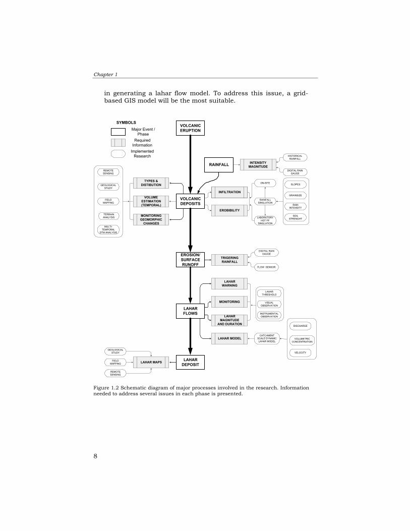
in generating a lahar flow model. To address this issue, a grid-based GIS model will be the most suitable.
Figure 1.2 Schematic diagram of major processes involved in the research. Informationneeded to address several issues in each phase is presented.
VOLCANICERUPTION
VOLCANICDEPOSITS
EROSION/SURFACERUNOFF
RAINFALL
LAHARFLOWS
LAHARDEPOSIT
REMOTESENSING
FIELDMAPPING
TERRAINANALYSIS
GEOLOGICALSTUDY
REMOTESENSING
CATCHMENTSCALE DYNAMICLAHAR MODEL
HISTORICALRAINFALL
MULTI-TEMPORAL
DTM ANALYSIS
FLOW SENSOR
RAINFALLSIMULATION
INTENSITYMAGNITUDE
TYPES &DISTIBUTION
VOLUMEESTIMATION(TEMPORAL)
TRIGERINGRAINFALL
MONITORING
EROBIBILITY
LAHAR MODEL
MONITORINGGEOMORPHIC
CHANGES
LAHARWARNING
LAHARMAGNITUDE
AND DURATION
FIELDMAPPING
GEOLOGICALSTUDY
LABORATORYHOT PF
SIMULATION
ON-SITE
DIGITAL RAINGAUGE
DIGITAL RAINGAUGE
SYMBOLSMajor Event /
PhaseRequired
InformationImplemented
Research
LAHAR MAPS
EROBIBILITY
INFILTRATION
SLOPES
RAININTENSITY
GRAINSIZE
SOILSTRENGHT
DISCHARGE
VOLUMETRICCONCENTRATION
VELOCITY
VISUALOBSERVATION
INSTRUMENTALOBSERVATION
LAHARTHRESHOLD

Introduction
9
1.5 Objectives of the research
Based on the foregoing considerations, the following research objectives were defined: • To study geomorphologic changes in watersheds affected by
extensive pyroclastic flow accumulation, considering such aspects as erosion, secondary pyroclastic flows, landslides and stream piracy.
• To develop a method for the rapid assessment of pyroclastic flow
and lahar deposits, using multi-temporal satellite images to complement field-based methods.
• To quantify the volume of pyroclastic flow material and the
amount of subsequent yearly erosion, using multi-temporal DTMs.
• To demonstrate the significant effects of secondary explosions
and stream capture that occurred in the catchments. • To study the lahar-triggering rainfall thresholds and their
variations through time in order to improve lahar warning. • To establish any relationships between rainfall intensity and
duration, and erosion intensity on pyroclastic flow deposits. This will contribute to the understanding of lahar flow initiation.
• To study the infiltration and runoff of in situ pyroclastic flow
deposits, lahars and ashfall, using a portable rainfall simulator. • To understand the rheologic characteristics of lahars as a
function of sediment supply and delivery, and to evaluate the changes over a period of several years after an eruption.
• To develop a lahar flow simulation model using a cell-based
dynamic physical GIS software. The lahar model will give some understanding on the magnitude and duration of lahar flow given certain amount of rainfall, and can be an important tool for lahar prediction in other areas.
1.6 Research methodology
Several research methods have been used to accomplish the different objectives mentioned in section 1.5. A more detailed description of the different methods can be found in each chapter.

Chapter 1
10
An overview of the major components of this research is presented in Figure 1.2. The flow diagram depicts the major events and the corresponding research applied to address several issues. The following methods were used in this research: • Several SPOT and Landsat TM images were used to study the
synoptic changes in the geomorphology and vegetation in the whole Mt. Pinatubo area from pre-1991 eruption to year 2000.
• For the detailed study area, mapping and monitoring geomorphic
changes were carried out by interpreting oblique and vertical aerial photographs. Erosion was rapidly assessed using stereoscopic interpretation and photogrammetric methods in order to estimate channel erosion. Field verifications were carried out during the two fieldwork campaigns.
• Several GIS software packages were used in the quantitative analysis of erosion rates, with the aid of multi-temporal DTMs. Several DTMs produced by various organizations were incorporated in the analysis.
• Telemetric networks of rain gauges and flow sensors were
installed in the upper watershed. Large amounts of data were collected from several sensors over a period of seven years. To automate data extraction, cleaning and analysis, visual basic programs using macros were created. Statistical software was used to model lahar-triggering rainfall thresholds. Rainfall lahar thresholds were analyzed for each year since the scale of geomorphic changes affects the yearly thresholds.
• A portable rainfall simulator was used to study the hydraulic
properties and erosivity of the different Mt. Pinatubo deposits. Emphasis was given to the 1991 pyroclastic flow materials since it is the major source of erodible material. Different parameters were studied in the model that affects infiltration and runoff i.e., various rainfall intensities and slope angles.
• Statistical regression modelling was applied to the infiltration and
runoff data acquired in the rainfall simulator experiments, in order to study the behaviour of the different parameters.
• A dynamic GIS was used to develop a lahar flow simulations. The
model is a distributed physical-based model that simulates continuously lahar flow calculating the volumetric concentration, velocity and discharge in three watersheds. Several catchment’s physical parameters were taken into account.

Introduction
11
• Several active lahar measurements were conducted in the field in order to validate the results of the lahar model.
1.7 Test area
Mt. Pinatubo serves as an excellent open-air laboratory to conduct this research on pyroclastic flow deposits, their rapid erosion, and resulting lahars. Depending on the type of analysis, different study scales were used: regional scale for the application of remote sensing; watershed scale for rainfall and lahar studies; micro-plot scale for determining the relative erosivity of the different deposits. A description of the study area is presented in Chapter 3.
1.8 Thesis chapter organization
This thesis is composed of eight chapters. Chapter 1 is an introductory chapter describing the objectives of this research. Chapter 2 discusses the current understanding on pyroclastic flow erosion and lahar processes. In Chapter 3 an introduction is given to the study area. Chapter 4 gives an overview of the 1991 eruption, and demonstrates the use of remote sensing data for monitoring the pre-eruption and post-eruption changes in the area, related to erosion and the development of the lahar accumulation over several years. Chapter 5 deals with the quantitative analysis of the volume of the 1991 pyroclastic flow deposits and the analysis of the yearly erosion rates in the Sacobia watershed, using several DTMs. It also discusses the accuracy and limitations involved when using different sources of DTM data. Chapter 6 deals with an extensive analysis of rainfall and flow sensor data. Statistical analyses of lahar-triggering rainfall thresholds are presented, which can be used as a tool in forecasting lahars. Chapter 7 describes the results of determining the in situ hydraulic conductivity and erosivity of the different Mt. Pinatubo deposits, using a portable rainfall simulator. Simulated rainfall tests with variable intensities and measured runoff were carried out on several test sites, with slopes ranging from 20 to 100%. Rainfall simulations were also conducted in the laboratory on pre-heated pyroclastic flow deposits. Chapter 8 describes the modelling results for lahar initiation, using a cell-based dynamic GIS model. And the last chapter, Chapter 9, gives the summary and conclusions of the research. It also presents the significant findings and makes research recommendations for future research.

Chapter 1
12

Lahar Types and Processes
13
Chapter 2 : Lahar Types and Processes 2.1 Introduction The word “lahar” comes from Java, Indonesia, and was introduced by Scrivenor (1929) when describing the flows (mudstream) from the crater lake at Kelut Volcano in East Java. Van Bemmelen (1949) later broadened the definition into “a mudflow containing debris and angular blocks (volcanic breccia) of chiefly volcanic origin transported by water”. The International Association of Volcaniclastic Sedimentologists further defined lahar as “a rapidly flowing mixture of rock debris and water, other than a normal stream flow, from a volcano” (Smith and Fritz, 1989). After nearly every volcanic eruption that produces extensive ashfall and pyroclastic flow deposits, massive erosion and lahar deposition will take place for several years (Yokohama, 1999; Major et al., 2000). Resulting lahars may produce more widespread devastation at the foot of the volcano than the main eruption itself. This chapter will discuss the current understanding about lahars as gained from studying different volcanoes, from lahar initiation to deposition. In the later part of the chapter, discussion will focus on Mt. Pinatubo lahars. 2.2 Sources of lahars and scale of erosion on volcanoes 2.2.1 Sources of lahars All loose sediments, from very fine to huge boulders, deposited on the slopes of a volcano are potential sources of lahars. Lahars that are triggered by rain initially mobilize finer sediments (clay to gravel size) and bulk up downstream as more sediments are entrained. Whiting et al. (1999) observed that progressively coarser sediment could be expected at higher discharges. These particles move as wash load, suspended load and/or bed load, depending upon stream energy. As the density of the flow increases, they have the capability to pick up boulders, which can remain suspended during the flow. Rodolfo (1989) likewise observed that lahars significantly grew in volume by eroding their channels. Most sources of fine sediments are loose tephra and pyroclastic flow deposits in particular, irrespective of their age. If the surface is bare and unprotected, non-welded ignimbrite (Figure 2.1) usually suffers very intense erosion by water flow. Many river terraces and reworked ignimbrites that have developed extensively in non-

Chapter 2
14
welded ignimbrite fields are interpreted as the products of such rapid dissection (Yokohama, 1999).
2.2.2 Scale of erosion on volcanoes Catchment environments are normally exposed to various degrees of erosion. The magnitude of erosion is dependent on many factors, such as catchment size and configuration, slope steepness and length, amount of vegetation cover, abundance and grain sizes of erodible materials, infiltration capacity, soil cohesion, existing erosion control structures and agricultural practices. The eroding agent, whether it is rainfall, breached impounded water and/or snowmelt, has great influence on the volumes of material that could be eroded. Catchments that have been extensively used for agriculture or recently cultivated have erosion rates ranging from tens to hundreds of tons/km2/year, which is significantly less erosion than on volcanoes that produce lahars. Catchments on volcanoes with large amounts of
Figure 2.1. Depositional mechanism of vent-derived pyroclastic flow deposits. Fig. (a)depicts how eruption column collapse could generate pyroclastic flow deposits; Fig. (b)shows the lateral propagation of pyroclastic flows, which can overtop drainage divides;Fig. (c) shows the condition of pyroclastic flow deposits after vent-derived pyroclastic flowceases. Renewed secondary explosion from primary pyroclastic flow deposits triggeredsecondary pyroclastic flows redistributing deposits downstream.

Lahar Types and Processes
15
newly deposited material, such as on Mt. Pinatubo, might have erosion rates as high as a million tons/km2/year (Hayes, 1999; Hayes et al., 2002). Figure 2.2 compares the erosion rates of two such volcanic catchment environments with those from other rivers.
Figure 2.2. Comparative scales of erosion of different catchment environments (afterHayes, 1999).

Chapter 2
16
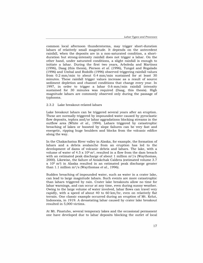
2.3 Lahar triggering mechanism Lahars are triggered by several mechanisms, such as: (1) rainfall; (2) the release of impounded water from a crater lake or a lahar-dammed lake by either a sudden breach or a small eruption from a volcano; (3) melting snow caused by hydrothermal heating on the peak of the volcano or the deposition of hot pyroclastic flows or lava flows; and (4) in some cases by landslides or avalanches − sometimes earthquake-induced (Pierson, 1998). Such lahars may occur not only before or during eruptions, but also during volcanically quiet (and seemingly safe) periods (Pierson, 1998; Kerle, 2001). 2.3.1 Rain-triggered lahars Most lahar events are triggered by rainfall. Though these generally have a smaller magnitude than other triggering mechanisms, their frequency of occurrence is far higher, especially in the tropics. Some examples of rain-triggered lahars can be found at Mt. Pinatubo (Pierson et al., 1996) and Mayon Volcano (Rodolfo, 1989; Rodolfo and Arguden, 1991) in the Philippines, and Mt. Kelud (Thouret et al, 1998) and Merapi Volcano (Lavigne et al, 1998) in Indonesia. Lahars are initiated when a sufficient amount of rain falls within a certain duration of time. Intensity and duration of rainfall are the most critical factors controlling the initiation of lahars. For example, at Merapi Volcano an average rainfall intensity of 0.33 mm/min sustained for two hours can initiate lahars (Lavigne, et al., 996). Likewise, at Mt. Pinatubo lahars were triggered by rainfall of more than 0.3 mm/min sustained for 30 minutes in 1992 (Tungol and Regalado, 1996) and about 0.6 mm/min sustained for 30 minutes in 1997 (Chapter 6, this thesis). Mayon lahars were triggered by rainfall of more than 0. 6 mm/min in 30 minutes (for debris flow) in the initial years − figures significantly higher than those for Merapi and Mt. Pinatubo during the initial years (Rodolfo and Arguden, 1991). Excessive rainfall can also trigger catastrophic lahars even decades after the last eruption (Kerle and de Vries, 2001). An example is Casitas Volcano in Nicaragua; Hurricane Mitch produced rainfall of 700 mm in 48 hours, resulting in an avalanche of approximately 200,000 m3 that led to lahars downstream, killing approximately 2,500 people. 2.3.1.1 Rain-triggered lahars at Mt. Pinatubo Most lahar events at Mt. Pinatubo are triggered by rainfall. The lahar magnitude is related to the intensity and duration of rainfall, as well as the volume and type of easily erodible source materials, the hydrologic properties and the antecedent rainfall. Short rainfall bursts, such as the
Lahar Types and Processes
17
common local afternoon thunderstorms, may trigger short-duration lahars of relatively small magnitude. It depends on the antecedent rainfall, when the deposits are in a non-saturated condition, a short-duration but strong-intensity rainfall does not trigger a lahar. On the other hand, under saturated conditions, a slight rainfall is enough to initiate a lahar. During the first two years, Arboleda and Martinez (1996), Daag (this thesis), Pierson et al. (1996), Tungol and Regalado (1996) and Umbal and Rodolfo (1996) observed triggering rainfall values from 0.2 mm/min to about 0.4 mm/min sustained for at least 30 minutes. These rainfall trigger values increase as a result of source sediment depletion and channel conditions that change every year. In 1997, in order to trigger a lahar 0.6 mm/min rainfall intensity sustained for 30 minutes was required (Daag, this thesis). High magnitude lahars are commonly observed only during the passage of typhoons. 2.3.2 Lake breakout-related lahars Lake breakout lahars can be triggered several years after an eruption. These are normally triggered by impounded water caused by pyroclastic flow deposits, tephra and/or lahar aggradations blocking streams in the outflow area (White et al., 1994). Lahars triggered by catastrophic breaching of lakes or boosted by slope failures can be very fast and energetic, ripping huge boulders and blocks from the volcanic edifice along the way. In the Chakachatna River valley in Alaska, for example, the formation of lahars and a debris avalanche from an eruption has led to the development of dams of volcanic debris and lahars. The lake, with a volume of water of 4.5 x 10⁸ m3, resulted in a flow from the dam breach with an estimated peak discharge of about 1 million m3/s (Waythomas, 2000). Likewise, the failure of Aniakchak Caldera (estimated volume 3.7 x 10⁹ m3) in Alaska resulted in an estimated peak discharge greater than 1.1 million m3/s (Waythomas et al., 1996). Sudden breaching of impounded water, such as water in a crater lake, can lead to large magnitude lahars. Such events are more catastrophic than lahars triggered by rain. Crater lake breakouts allow no time for lahar warnings, and can occur at any time, even during sunny weather. Owing to the large volume of water involved, lahar flows can travel very rapidly, with a speed of about 40 to 60 km/hr, even on relatively flat terrain. One classic example occurred during an eruption of Mt. Kelut, Indonesia, in 1919. A devastating lahar caused by crater lake breakout resulted in 5,000 victims. At Mt. Pinatubo, several temporary lakes and the occasional permanent one have developed due to lahar deposits blocking the outlet of local
Chapter 2
18
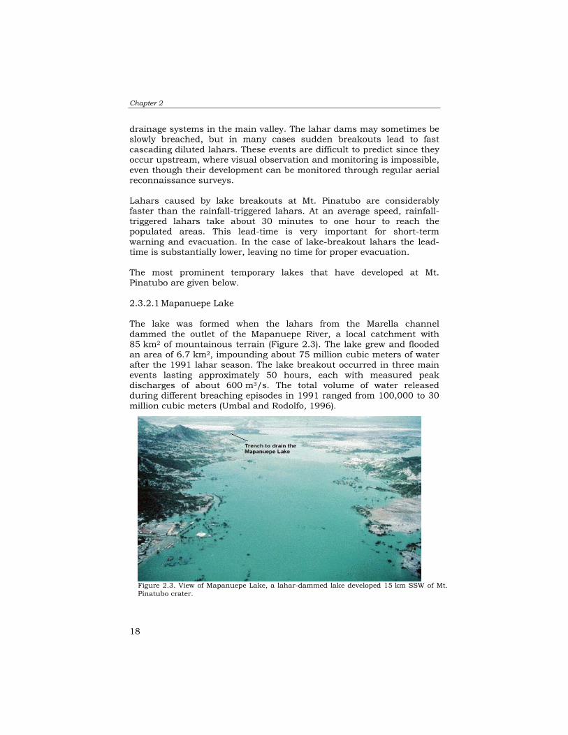
drainage systems in the main valley. The lahar dams may sometimes be slowly breached, but in many cases sudden breakouts lead to fast cascading diluted lahars. These events are difficult to predict since they occur upstream, where visual observation and monitoring is impossible, even though their development can be monitored through regular aerial reconnaissance surveys. Lahars caused by lake breakouts at Mt. Pinatubo are considerably faster than the rainfall-triggered lahars. At an average speed, rainfall-triggered lahars take about 30 minutes to one hour to reach the populated areas. This lead-time is very important for short-term warning and evacuation. In the case of lake-breakout lahars the lead-time is substantially lower, leaving no time for proper evacuation. The most prominent temporary lakes that have developed at Mt. Pinatubo are given below. 2.3.2.1 Mapanuepe Lake The lake was formed when the lahars from the Marella channel dammed the outlet of the Mapanuepe River, a local catchment with 85 km2 of mountainous terrain (Figure 2.3). The lake grew and flooded an area of 6.7 km2, impounding about 75 million cubic meters of water after the 1991 lahar season. The lake breakout occurred in three main events lasting approximately 50 hours, each with measured peak discharges of about 600 m3/s. The total volume of water released during different breaching episodes in 1991 ranged from 100,000 to 30 million cubic meters (Umbal and Rodolfo, 1996).
Figure 2.3. View of Mapanuepe Lake, a lahar-dammed lake developed 15 km SSW of Mt.Pinatubo crater.

Lahar Types and Processes
19
After the lake breakout in 1991, the lake was re-formed and grew to as much as 9.2 km2 in 1995. Maximum depth of the lake was about 20 m at an elevation of 120 masl (Calomarde, 1997). 2.3.2.2 Pasig Lake This lake started to develop when lahars from the main Pasig channel obstructed the outlet of the 24 km2 Yanca sub-catchment (local catchment). Pasig Lake occupied a maximum area of around 8 km2 (Figure 2.4).
A breakout of the lake occurred twice, delivering fast cascading diluted lahars in 1992 and in 1994. The lahars produced during these events had a different rheology and clast content, since the source materials were mostly scoured from the pre-1991 channel materials. (Figure 2.5).
Figure 2.4. Photo of the lake in Pasig River, which was developed byaggrading lahar deposits at the outlet.

Chapter 2
20
2.3.3 Lahars triggered by snowmelt Thick snow capping the edifice of the volcano can serve as a natural source of excessive water, which when melted can generate devastating lahars. A recent catastrophic example is the 13 November 1985 Nevado Del Ruiz Volcano eruption in Colombia. A relatively small eruption generating a pyroclastic flow and phreatic explosions melted the snow and ice on the top of the volcano and initiated a lahar. The lahar travelled about 100 km at a speed of 60 km/hr on the upper slopes and killed 23,000 people in the city of Armero (Pierson et al., 1990). Cronin et al (1995) also described the lahars generated by Ruapehu Volcano in New Zealand; phreatic and phreato-magmatic eruptions forced the release of the crater lake. Crater lake water, sediment and juvenile material were incorporated with snow and ice to form “snow slurry” lahars. A small amount of water was enough to mobilize a large amount of snow. Bovis and Jacob (2000) also noted that extreme hot weather could induce ice caps to melt, causing landslides leading to lahars.
Figure 2.5. Lake-breakout lahar deposits(bottom section) showing lithic rich clasts thatwere scoured from the pre-1991 deposits.
Lahar Types and Processes
21
2.3.4 Landslides leading to lahars Rapid wet (but unsaturated) granular flows, usually classified as debris avalanches (Pierson and Costa, 1987), commonly begin as large landslides from the flanks of volcanoes. These phenomena can involve volumes of debris up to several tens of cubic kilometres, and can travel at velocities as high as 360 km/hr (Siebert, 1992). 2.4 Type and characteristics of lahars Lahars are composed of rocks, ash and water, with a consistency similar to wet concrete. They can exert pressures approaching 106 kg/m2 (Rodolfo, 2000 in Kerle and van Wyk de Vries, 2001). Beverage and Culbertson (1964) and Costa (1984) made a subdivision of lahars, based on the rheology of the flows, into debris flows and hyperconcentrated flows. Transition from debris flow to hyperconcentrated flow, and vice versa can commonly occur. Further dilution of hyperconcentrated flow can lead to muddy stream flow and then to normal stream flow, which are not considered lahars due to their low sediment content (Smith and Fritz, 1989). Lahar rheology is important in hazard assessment. For example, cohesive lahars, non-cohesive lahars and debris avalanches exhibit different flow behaviours. Cohesive lahars spread much more widely than non-cohesive lahars that have travelled similar distances. Cohesive lahars also travel farther and spread wider than debris avalanches of similar volume (Vallance and Scott, 1997). 2.4.1 Debris flow Debris flows are gravity-driven highly concentrated mixtures of sediment and water that have a very high yield strength (Pierson and Costa, 1987). Their motion is driven by inertial forces that induce grain friction and grain collisions by sediment-laden stream flow as they mix with stream water along their paths (Pierson and Scott, 1985). Debris flows are non-Newtonian fluids that move as coherent masses with a sediment concentration exceeding 60% in volume and 80% in weight. There are two general types of debris flow, based on the amount of water when they are initiated. The first type is when a debris flow is initiated in a relatively dry state by a landslide or avalanche. Such conditions occur in steep mountainous regions. Another type of debris flow occurs when flows are initiated and sustained by water. Typical examples are debris flows from volcanoes or in areas with high rainfall. Debris flows from avalanches, even extremely large ones, typically do not travel more than several tens of kilometres away from their sources,
Chapter 2
22
despite their great bulk and initial speed, unless they become water-saturated (Pierson, 1998). There is evidence that debris avalanches stop very abruptly (Siebert, 1996; Major and Iverson, 1999), apparently due to the “locking up” of the coarse angular debris during deceleration. Water-saturated debris flows are more mobile because positive pore-fluid pressures greatly decrease internal friction within the debris mass (Pierson and Costa, 1987). Debris flows can flow as fast as 150 km/hr and are capable of flowing hundreds of kilometres down valleys away from their sources (Pierson, 1998). Erosion and the incorporation of sediment by flowing water on the steep upper slopes of volcanoes typically result in large increases in flow volume. On the other hand clay-rich (cohesive) debris flows can travel great distances with little or no change in rheology (Johnson, 1984; Pierson and Costa, 1987; Pierson, 1998). Water-saturated debris flows have a flow behaviour distinct from hyperconcentrated flows and muddy stream flows, and can be characterized as laminar and clast-rich. Huge boulders and other heavy objects can remain suspended during flow owing to the high density of the flow. A very audible low frequency sound (rumbling) can be heard, which can be a natural sign of approaching debris flow. Mt. Pinatubo debris flows have been observed from 1991 to 1995. They have a high sediment concentration, as much as 85% in volume (Rodolfo et al., 1996), and flow in a laminar fashion, often transporting chunks of hot pyroclastic materials. Such flows are less turbulent due to the increase in sediment content (Rodolfo et al., 1996). Flow density of slurries ranges from 1.8 to 2.3 g/cm3, but density of flows that are lithic-rich ranges from 2.4 to 2.7 g/cm3 (Pierson et al., 1996). Because of its high density, the flow can destroy bridges by an upward lifting force (buoyant force) rather than by horizontal impact, as demonstrated by the destruction of Bamban bridge in 1991. From near-bank observation of debris flows on Mt. Pinatubo, it was concluded that such events can produce very audible sounds during flow. When flow is relatively quiet, sediment bed load is composed mainly of sand-size particles. In many cases, flows rich in boulders produce an internal rumbling sound (low frequency sound) as a result of clashing boulders during transport. This characteristic sound is often an audible warning to villagers in the area that a lahar is ongoing. Occasionally, steam explosions within debris flows can be observed; this is due the rapid steam expansion when water comes in contact with hot chunks of pyroclastic flows. Flow velocities can range from 3 m/s to about 10 m/s when observed in a relatively flat area (~1°). Peak discharge can have an average of about 200 m3/s during a moderate
Lahar Types and Processes
23
lahar to around 1,100 m3/s during a strong lahar flow (Martinez et al., 1996, Tungol and Regalado, 1996). 2.4.2 Hyperconcentrated flow Hyperconcentrated flows have a lower sediment concentration, ranging from 20 to 60% in volume and 40 to 80% in weight (depending on grain size distribution), overlapping in range with debris flows (Pierson and Costa, 1987). Hyperconcentrated flows are dense suspensions of sediment in water, but concentrations are low enough for coarser sediment particles to be able to settle out of suspension when flow velocities decrease. These flows appear more viscous than the normal concentration stream flow (Janda et al., 1996; Pierson and Costa, 1987). Flow is characteristically turbulent, but some turbulence is dampened by the higher fluid viscosity (Beverage and Culbertson, 1964; Pierson and Scott, 1985). Hyperconcentrated sediment/water mixtures possess a low yield strength (Smith and Lowe, 1991), and normal-density gravel is not carried in suspension as it is in debris flows. Hyperconcentrated flows observed at Mt. Pinatubo are more turbulent than debris flows. Their concentration is relatively low, making the coarse sediment particles settle out of suspension, especially when velocity is decreased. Flow densities are lower than in debris flow, with values around 1.20 to 1.35 g/cm3 (Rodolfo et al., 1996). These flows are highly erosive, both laterally and vertically, and they produce an audible higher frequency sound comparable to ocean surf, due to the presence of standing waves. Waveforms of dunes and anti-dunes in the flow are common. Measured velocities on gentle slopes (<1°) are about 3 to 6 m/s. On steeper slopes it is assumed that flow velocities are much higher, but this cannot be proven as no measurements have been made in the inaccessible river valleys. Temperatures are generally lower due to a water content higher than in a debris flow, but temperatures around 35°C have still been recorded 2.5 Lahar sedimentology 2.5.1 Active lahars at Mt. Pinatubo Active lahars were studied at Mt. Pinatubo in terms of their grain sizes. Several active lahars ranging from debris flow, hyperconcentrated flow to muddy stream flow were sampled in the field at various locations. Figure 2.6 is a graph showing the cumulative grain size distribution of different samples taken during the actual flow. This figure shows that debris flows (shown as thick lines) have a median grain size of coarse to medium sand (-1 to 1 phi) and about 25% (in weight) of each sample has a grain size of gravel to coarse sand (-2.5 to –1 phi).

Chapter 2
24
Compared with debris flow samples, hyperconcentrated flows (represented as thin lines) have more fine-grained sediments. Median grain size of these sediments is in the range of medium to fine sand (1 to 3 phi). Muddy stream flow (plotted as dotted lines) shows a median grain size of silt (4 phi). From the different active lahar samples collected, it appears that most of the deposits are rich in sand (median grain size is coarse to fine sand) since the sandy pyroclastic flow is the main source material. Different field conditions of active lahars are presented in Figures 2.7 and 2.8.
Figure 2.7 Debris flow as observed in Sacobia River: (A) laminar flow, and (B) turbulentstanding wave, which is rarely observed in a debris flow. Flow temperatures are in theorder of 40 to 50°C. After Pierson et al. (1996).
GRAINSIZE OF ACTIVE LAHAR
0
10
20
30
40
50
60
70
80
90
100
-4.0 -3.5 -3.0 -2.5 -2 -1.5 -1.0 -0.5 0.0 0.5 1.0 1.5 2.0 2.5 3.0 3.5 4.0 > 4.0
GRAIN SIZE in PHI UNIT
CU
MU
LATI
VE W
EIG
HT
(%)
Figure 2.6. Grain size distribution of debris and hyperconcentrated flows sampled duringactive lahar flow (thick lines represent debris flow, solid thin lines representhyperconcentrated flow, and dotted lines represent muddy stream flow).
Lahar Types and Processes
25
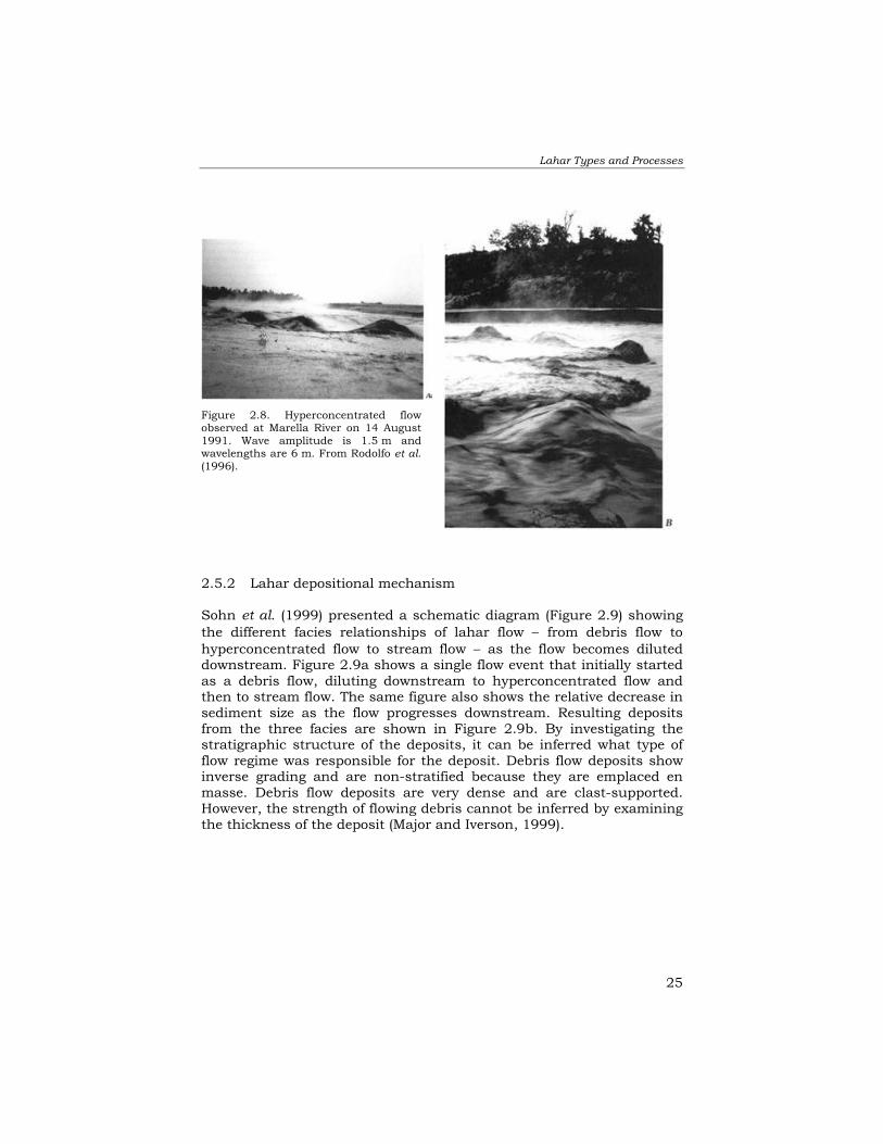
2.5.2 Lahar depositional mechanism Sohn et al. (1999) presented a schematic diagram (Figure 2.9) showing the different facies relationships of lahar flow − from debris flow to hyperconcentrated flow to stream flow − as the flow becomes diluted downstream. Figure 2.9a shows a single flow event that initially started as a debris flow, diluting downstream to hyperconcentrated flow and then to stream flow. The same figure also shows the relative decrease in sediment size as the flow progresses downstream. Resulting deposits from the three facies are shown in Figure 2.9b. By investigating the stratigraphic structure of the deposits, it can be inferred what type of flow regime was responsible for the deposit. Debris flow deposits show inverse grading and are non-stratified because they are emplaced en masse. Debris flow deposits are very dense and are clast-supported. However, the strength of flowing debris cannot be inferred by examining the thickness of the deposit (Major and Iverson, 1999).
Figure 2.8. Hyperconcentrated flowobserved at Marella River on 14 August1991. Wave amplitude is 1.5 m andwavelengths are 6 m. From Rodolfo et al.(1996).

Chapter 2
26
Sohn et al. (1999) describe the unchannelized debris flows as having (1) sheet-like or lobate geometry, (2) non-erosional bases, (3) poor sorting, (4) relatively minor silt and only traces of clay-sized ash, (5) either matrix or clast support, and (6) common outsized clasts at their tops. The inverse graded debris flow deposits are thick, suggesting a lack of cohesion and considerable dispersive pressure; they have long clast axes aligned parallel to bedding due to strongly sheared laminar flow. Hyperconcentrated flow deposits are characterized by (1) coarse sand to fine gravel textures, (2) poor sorting, (3) faint horizontal bedding that is thicker than typical fluvial laminae, (4) absence of cross-bedding, and (5) intrastratal occurrence of small gravel lenses or outsized gravel clasts. They have less packing density and are less indurated compared with debris flows, since their fine particles (silt and clay) are rather depleted. All of these features suggest rapid deposition from suspension or traction (Pierson and Scott, 1985; Major et al., 1996). 2.5.3 Stratigraphy of Mt. Pinatubo lahars The 1991 Mt. Pinatubo deposits contained high proportions of lower-density pumice but their volumetric sediment concentrations were similar to all other types of lahars. The stratigraphic descriptions are divided into two parts: one on debris flow deposits and the other on hyperconcentrated flow deposits. 2.5.3.1 Debris flow deposits Debris flow deposits are massive as there is little time for sorting before being deposited. As a result, the deposits are poorly to extremely poorly sorted. They generally have massive internal structures (lack of internal stratification) and sometimes they have inverse grading due to the
Figure 2.9. Schematic diagram: (a) shows different phases of lahar flows, from debris flowto hyperconcentrated flow to stream flow; (b) shows the sedimentologic structure that canbe observed on the deposits (after Sohn et al., 1999).

Lahar Types and Processes
27
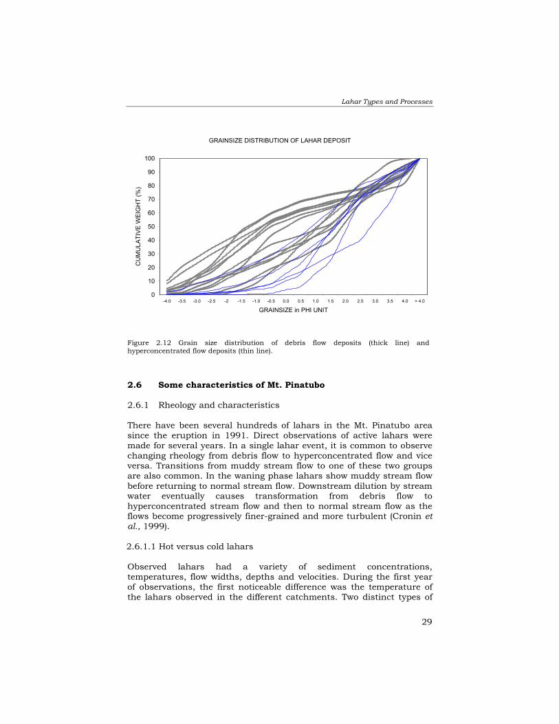
presence of light coarse pumice materials. They are densely packed and consolidated, and the weight percentage of fine particles is nearly similar to that of the source materials. The exceptionally large clasts are mostly matrix-supported as a result of suspension in the high-density matrix (Figure 2.10). Depending on the lahar event, if the source sediment is the 1991 pyroclastic flow deposit the material is generally sandy (Figure 2.11). However, in the case of lake breakout lahars, the average grain size is much larger due to the presence of large clasts scoured from the pre-1991 deposits. Sometimes the massive sedimentary structures of debris flows resemble pyroclastic flow deposits. But they can be distinguished because their clasts do not have a consistent orientation − a result of remobilization and colder emplacement temperature. Another way to distinguish them in the field is by their degree of compaction. Since debris flows were remobilised by water, their deposits are more compact than pyroclastic flow deposits, and hence more resistant to rain erosion. The difference in the degree of compactness can lead to the differentiation between pyroclastic flow and debris flow deposits. 2.5.3.2 Hyperconcentrated flow deposits Hyperconcentrated flow deposits are poorly sorted and horizontal bedding is rare or, if present, very faint. Cross-bedding is absent but small gravel lenses can be found. Their depositional features are very different from those of a normal stream flow and suggest rapid deposition. Figure 2.12 shows the grain size distribution of debris and hyperconcentrated flow deposits gathered in the field. It also appears that debris flow deposits (represented by a thick line) have a median grain size between gravel and medium sand (-2 to 1.5 phi), while hyperconcentrated flow deposits (represented by a thin line) are in the range of medium to fine sand (1 to 3.5 phi).
Chapter 2
28
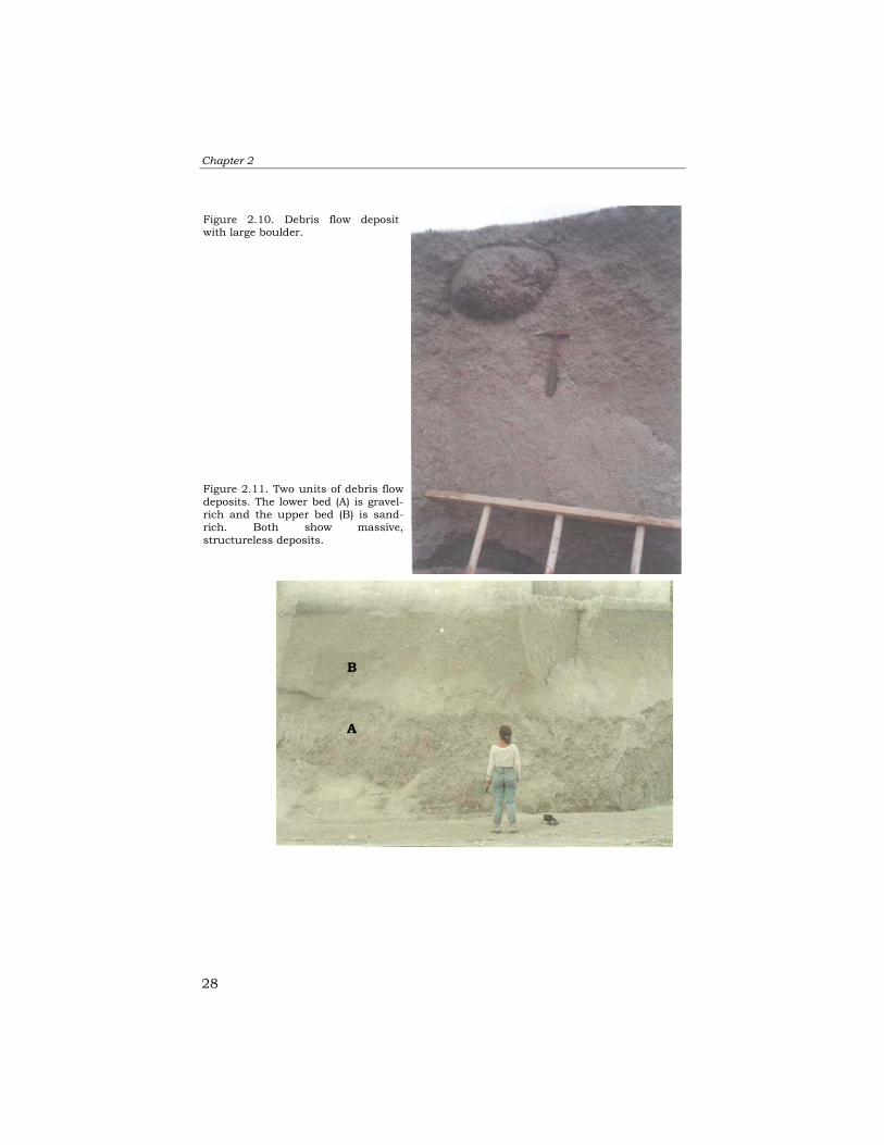
Figure 2.11. Two units of debris flowdeposits. The lower bed (A) is gravel-rich and the upper bed (B) is sand-rich. Both show massive,structureless deposits.
Figure 2.10. Debris flow depositwith large boulder.
B
A
Lahar Types and Processes
29
2.6 Some characteristics of Mt. Pinatubo 2.6.1 Rheology and characteristics There have been several hundreds of lahars in the Mt. Pinatubo area since the eruption in 1991. Direct observations of active lahars were made for several years. In a single lahar event, it is common to observe changing rheology from debris flow to hyperconcentrated flow and vice versa. Transitions from muddy stream flow to one of these two groups are also common. In the waning phase lahars show muddy stream flow before returning to normal stream flow. Downstream dilution by stream water eventually causes transformation from debris flow to hyperconcentrated stream flow and then to normal stream flow as the flows become progressively finer-grained and more turbulent (Cronin et al., 1999). 2.6.1.1 Hot versus cold lahars Observed lahars had a variety of sediment concentrations, temperatures, flow widths, depths and velocities. During the first year of observations, the first noticeable difference was the temperature of the lahars observed in the different catchments. Two distinct types of
Figure 2.12 Grain size distribution of debris flow deposits (thick line) andhyperconcentrated flow deposits (thin line).
GRAINSIZE DISTRIBUTION OF LAHAR DEPOSIT
0
10
20
30
40
50
60
70
80
90
100
-4.0 -3.5 -3.0 -2.5 -2 -1.5 -1.0 -0.5 0.0 0.5 1.0 1.5 2.0 2.5 3.0 3.5 4.0 > 4.0
GRAINSIZE in PHI UNIT
CU
MU
LATI
VE W
EIG
HT
(%)

Chapter 2
30
lahar were observed: hot and cold. Lahars that originated from areas with 1991 pyroclastic flow deposits produced hot flows with temperatures measured up to 86°C. The average temperature of hot lahars is 40°C (Pierson et al., 1996; Umbal and Rodolfo, 1996). Almost all lahars that occurred from 1991 to about 1995, when the lahar channel was connected to the 1991 pyroclastic flow deposits, were considered hot lahars as their temperatures were above normal water temperature. In some catchments, only cold lahars were observed, and lahar activity lasted for only about two rainy seasons. Channels with cold lahars had tephra as their only source material. These tephra deposits are relatively small with thicknesses of about 15 to 50 cm in the upper catchment (Paladio-Melosantos et al., 1996) compared with the 100 m average thickness of the pyroclastic flow deposits. Cold lahars are generally hyperconcentrated. They have a lower volumetric sediment ratio than hot lahars. Arguden and Rodolfo (1990) noted that on hot flows the vaporization of water by heat from large clasts may have facilitated mobility by decreasing internal friction. Indirect velocity calculations indicate that hot lahars move faster and travel farther than cold flows. Although the different temperatures of active lahars have few implications for the rheology of the flow, perhaps the most vital information that can be extracted is that since cold lahars are not connected to the hot pyroclastic flow materials, it can be inferred that the long-term lahar threat for that catchment is significantly less. 2.6.2 Lahar frequency and magnitude Around Mt. Pinatubo lahars have occurred both during and after the 1991 eruption. Syn-eruption lahars were recorded during the height of the climactic eruption as it coincided with the arrival of Typhoon Diding (international name Yunya), causing heavy rainfall in the area. This caused massive destructive lahars that travelled some 40 km downstream of the volcano. Eyewitness accounts from people living 40 km downstream of the Pasig River described the arrival of a large destructive lahar as coinciding with the onset of the heavy tephra fall during the period of the climactic eruption (Daag, Jaime, pers. comm., 1991). The syn-eruption lahars simultaneously destroyed numerous bridges along the Pasig and Abacan channels, which rendered some vital roads impassable. During the month of August in 1991 approximately three to five lahar events occurred per day. On average they had a depth of 2 to 3 m, and a width of 20 to 50 m. Velocity ranged from 4 to 8 m/s and peak discharge varied from 200 to 1,200 m3/s. Some exceptionally large

Lahar Types and Processes
31
lahars were up to 5 m deep, with a velocity as high as 11 m/s and an estimated peak discharge of 5,000 m3/s (Pierson et al., 1996). Umbal and Rodolfo (1996) and Rodolfo et al. (1996) measured discharges of up to 2,000 m3/s on 29 July 1992 in the Santo Tomas River, which drains from the Marella catchment. Typical hydrographs of single-peak events have a left-skewed shape, with a sharper increase before the arrival of the peak flow and a slowly diminishing right limb before going back to normal muddy stream flow (Figure 2.13).
Several large devastating lahars occurred around Mt. Pinatubo from 1991 to 1995. Normally these destructive lahars occurred during the passage of typhoons accompanied by long-duration high-intensity rainfalls. An example of such a typhoon-related lahar is the event on 1 October 1995 in the Pasig-Potrero River caused by Typhoon Mameng (Arboleda and Martinez, 1996). During the passing of the typhoon, 337 mm of rain fell on the Sacobia pyroclastic fan, which triggered five distinct and fairly continuous lahar episodes over a 14-hour period. The largest episode, with an estimated peak discharge of 400 m3/s was observed in Mancatian, Porac. Hot lahars associated with steam were observed in the upper catchment but progressive dilution through the incorporation of older materials had cooled the flow down to ambient temperature by the time it reached the town of Minalin, located 40 km downstream. A total area of 25 km2, half of which was previously unaffected, was buried beneath 0.5 to 6 m of sediment. An estimated sediment volume of 50 million cubic meters was deposited during this event, with roughly 40% consisting of old pre-1991 eruption deposits and 60% of 1991 eruption lahar materials.
Figure 2.13. Figures showing the lahar hydrographs of two lahar events that occurredon (A) 28 June 1992 and (B) 29 July 1992 as observed in the Marella channel (fromRodolfo et al., 1996).

Chapter 2
32
2.7 Summary Erosion from recently erupted volcano produces several orders of magnitude compared to other catchment environments. This erosion causes lahar flows that pose a significant threat to life and property. Lahars can affect vast areas; burying settlements located several tens of kilometres downslope. Their occurrence is independent of the time of eruption. Lahars can be triggered by several mechanisms, i.e., rain, snowmelt, lake breakout, landslide and earthquake. Lahars triggered by lake breakout or melted snow are generally more dangerous because of the size and magnitude of the flows they generate. There are two types of lahar, i.e., debris flow and hyperconcentrated flow. Both are classified based on the sediment-to-water ratio that affects flow behaviour. Debris flows have higher sediment concentrations than hyperconcentrated flows. The sediment concentration of a debris flow exceeds 60% in volume and weight concentration exceeds 80%. At Mt. Pinatubo, most lahars are triggered by rainfall in excess of 0.3 mm/min sustained for 30 minutes. There have also been a number of devastating lake breakout lahar events. Lakes developed when the outlet was blocked by lahar deposits. Lahars observed during the first five years after the 1991 eruption were mostly hot, since their source sediments came from the still-hot 1991 pyroclastic flow deposits. In a single event, flows can have a variety of rheologies, i.e., debris flow, hyperconcentrated flow and muddy stream flow. Transitions between them are commonly observed. Median grain sizes of Mt. Pinatubo lahars are from medium to coarse sand, which are also similar to the median grain size of 1991 pyroclastic flow deposits.

Pinatubo Area
33
Chapter 3 : Pinatubo Area 3.1 Introduction This chapter aims to give an overview of the environmental setting of Mt. Pinatubo Volcano and the situation before the eruption of 1991. The June 1991 eruption and its post-eruption events are described in Chapter 4. The Philippines is one of the countries in the so-called Pacific Ring of Fire, the fringe surrounding the Pacific Ocean where numerous volcanic eruptions and large magnitude earthquakes occur. The country has at least 23 active and hundreds of inactive volcanoes. The Philippine Institute of Volcanology and Seismology (PHIVOLCS) initially categorizes a volcano as active if it has a written historical account of past eruptions. Archived written accounts in the Philippines only date back to around the 16th century, to the period of Spanish rule. As a result of this, several young and potentially active volcanoes with no historical records are still classified as inactive, and may pose an unrecognised danger in the future. PHIVOLCS has recently started a program for determining the age of the most recent prehistoric eruptions of these potentially active volcanoes by using radiocarbon dating. This study may result in the reclassification from inactive to active of a number of volcanoes with no historical eruption record if their volcanic deposits suggest a young morphology and C14 dating indicates an age less than a few hundred years old, just like Mt. Pinatubo. Mt. Pinatubo is located on the central part of Luzon (see Figure 3.7), the main island of the Philippines, at a distance about 120 km north of Manila. The volcano had an altitude of 1,745 meters above sea level (masl) prior to eruption, and the highest peak was centered at 15°08.8N and 120°21.1E (1675100N and 215500E UTM Zone 51). 3.2 Physiography In general, the Mt. Pinatubo area can be divided into two main physiographic units: “erosional highland” and “accumulational lowland”. The boundary between these two types of terrain can be drawn in the area where the volcano’s edifice terminates abruptly, which is at an elevation of around 200 masl. The highland terrain consists mostly of volcanic domes, pyroclastic flow terraces and deeply dissected valleys. The lowland terrain is the place where remobilisation and sedimentation of volcanic sediments has taken place and it consists mostly of numerous coalescing lahar and alluvial fans (Figure 3.1).

Chapter 3
34
West of Mt. Pinatubo are mountain ranges of ultramafic origin. Among them are: High Peak (2,037 m), Mt. Iba (1,670 m), Mt. Lunitan (1,320 m) and Mt. Redondo (611 m). These mountains have rounded peaks and smooth slopes. Vegetation growth consists largely of grasses to small shrubs. South of Mt. Pinatubo are two large young strato-volcanoes; these are Mt. Mariveles (1,365 m) and Mt. Natib (1,233 m), of which the latter has an age of only 1,000 years (Torres, 1994, oral comm.). The edifice of these volcanoes roughly measures 25 km in diameter. 3.2.1 Erosional highland terrains There are several older (pre-Pleistocene) andesitic volcanic domes and plugs that surround Mt. Pinatubo, such as Mt. Negron (1,583 m), Mt. Quadrado (1,324 m), Mt. Tayawan (1,470 m) and Mt. Donald McDonald (1,330 m). On the basis of petrographic studies (Daag et al., 1996; Newhall et al., 1996) it was concluded that these domes are remnants of the ancient (>35,000 years) Pinatubo volcanic complex. If reconstructed, the form of the ancient Pinatubo volcano might have had an elevation of 2,300 m before a calderagenic eruption took place, forming a caldera with a diameter of 5 km (Newhall et al., 1996). The size of the volcano’s edifice measured from its peak at 1,486 m down to the elevation of 200 m is about 40 x 40 km. At altitudes above 1,000 m, the volcano is surrounded by steep dissected mountains to the west, south and northeast. The catchments have slope angles that range from 20° to more than 45°. The average channel gradient is between 6° and 18°. At an altitude between 200 and 1,000 m highly eroded pyroclastic flow deposits can be found. The morphology of this area is characterized by badland terrain, with steep slopes (60 to 70°), knife-edged ridges, and a well-developed dendritic drainage pattern. There are isolated terraces where the pyroclastic flow deposits are capped by nearly horizontal and more resistant lahar materials that protect the underlying materials from erosion. The calderagenic eruption in 1991 reduced the former peak of 1,745 m to 1,486 masl (Jones and Newhall, 1996).
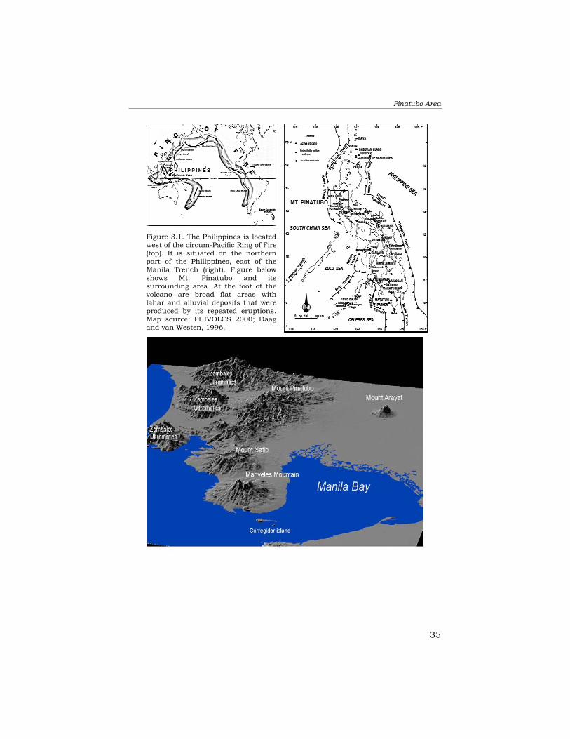
Pinatubo Area
35
Figure 3.1. The Philippines is locatedwest of the circum-Pacific Ring of Fire(top). It is situated on the northernpart of the Philippines, east of theManila Trench (right). Figure belowshows Mt. Pinatubo and itssurrounding area. At the foot of thevolcano are broad flat areas withlahar and alluvial deposits that wereproduced by its repeated eruptions.Map source: PHIVOLCS 2000; Daagand van Westen, 1996.
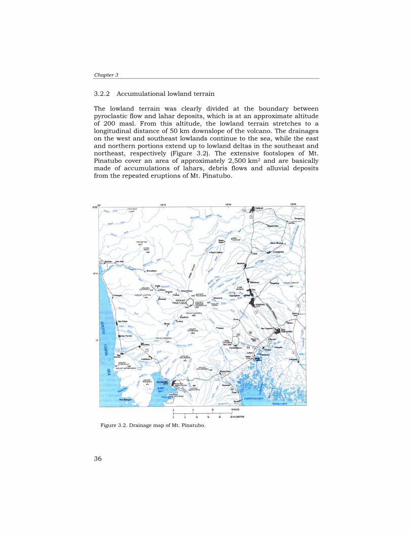
Chapter 3
36
3.2.2 Accumulational lowland terrain The lowland terrain was clearly divided at the boundary between pyroclastic flow and lahar deposits, which is at an approximate altitude of 200 masl. From this altitude, the lowland terrain stretches to a longitudinal distance of 50 km downslope of the volcano. The drainages on the west and southeast lowlands continue to the sea, while the east and northern portions extend up to lowland deltas in the southeast and northeast, respectively (Figure 3.2). The extensive footslopes of Mt. Pinatubo cover an area of approximately 2,500 km2 and are basically made of accumulations of lahars, debris flows and alluvial deposits from the repeated eruptions of Mt. Pinatubo.
Figure 3.2. Drainage map of Mt. Pinatubo.

Pinatubo Area
37
The upper part (from 200 to about 50 masl) consists mostly of numerous lahar terraces from lahar events from previous eruptions. On the lower part, the area is dominated by many broad coalescing alluvial fans with low gradients that range from about 2% near the apex of the fans to less than 0.02% on the distal parts. The low-lying areas are prone to perennial flooding. Currently, on this alluvial apron, all of the rivers have been (at least partly) artificially straightened and constrained by earthen dikes to mitigate flooding (Pierson et al., 1996). 3.3 Geology The geology of Mt. Pinatubo and its immediate vicinity is not only the product of volcanism (Figure 3.3). The mountain ranges located west of Mt. Pinatubo resulted from orogenic uplift of the Eocene South China oceanic floor during late Oligocene (Villones, 1980). This accretion process formed the Zambales Ophiolite Complex and is composed of mainly peridotite, basalt and gabbro (Villones, 1980; Delfin, 1983). Sedimentary and volcanic rocks can be found northeast and southeast of Mt. Pinatubo. The sedimentary rocks belong to the Askitero Formation that consists of a sequence of non-deformed and low dipping marine limestones and shales, which were uplifted during the late Miocene to early Pliocene (Villones, 1980). These sediments are also associated with non-marine and volcaniclastic sediments of the Tarlac Formation and are believed to unconformably overlie the Zambales Ophiolite Complex (Roque et al. 1972). The western part of Mt. Pinatubo is described by Javelosa (1994) as a system with very active uplifting in the Holocene period, as evidenced by several levels of raised beach ridges. The volcanic centers around Mt. Pinatubo are related to the subduction of the South China Sea Plate below the East Luzon Plate, which commenced in the Pleistocene epoch. Overlying the ophiolite sequence is a volcanic dome complex, with an age from Pliocene to Quarternary, and consisting of basaltic, andesitic and dacitic rocks. These can be found at Mt. Quadrado, Mt. Negron and Mt. Pinatubo (Villones, 1980). Mt. Pinatubo volcanism during the Pleistocene up to about 35,000 before present (BP) was more basaltic and andesitic with some dacite domes, associated with less explosive eruption types. Younger volcanism (<35,000 years BP) became more dacitic, resulting in increasingly explosive eruptions (Newhall et al., 1996).
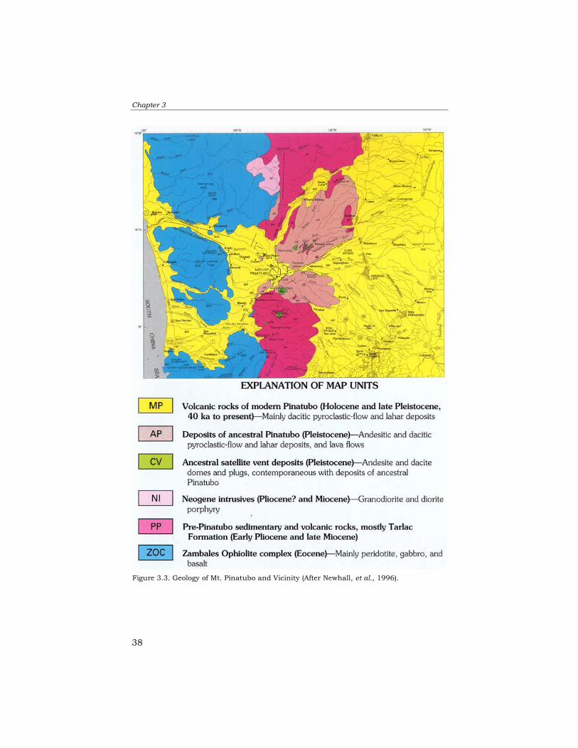
Chapter 3
38
Figure 3.3. Geology of Mt. Pinatubo and Vicinity (After Newhall, et al., 1996).
Pinatubo Area
39
Newhall et al. (1996) subdivided the history of Mt. Pinatubo into two periods, based on the changes in the magmatic composition and the relative age. These two periods are called “ancestral” and “modern” Pinatubo, while Delfin (1983) named them “old” and “young”. 3.3.1 Ancestral Pinatubo The rocks from the ancestral Pinatubo complex consist of basalt to andesite and some dacitic domes with an age ranging from 1 million years (early Pleistocene) to 35,000 years BP. Remnants from the volcanic activity of ancestral Pinatubo still dominate the landscape of the upper volcanic centers. Remnants of volcanic peaks from this period include Mt. Negron with a K-Ar age of 1.27 Ma and Mt. Cuadrado with a K-Ar age of 1.59 Ma (Bruinsma, 1983). Other volcanic domes and volcanic plugs related to ancestral Pinatubo are Mts. Mataba, Bituin and Tapungho. From these remnants it can be deduced that a younger caldera (belonging to the modern Pinatubo event) destroyed the ancestral dome in the area, which measured about 3.5 x 4.5 km. Its crater wall remnants could be traced from the patches of high resistant terrain, which include Mt. Donald McDonald, Mt. Tayawan, and also the slopes of Mt. Dorst and Mt. Kamanggi (Newhall et al., 1996). Debris flow and lahar deposits from ancient Pinatubo have significantly different characteristics from the modern Pinatubo lahars. Outcrops show clast-supported well-indurated layers with clast mostly of basalt and andesite. Much of the deposits on the lower footslopes have been covered by the younger deposits from the modern Pinatubo complex. 3.3.2 Modern Pinatubo The landscape around Mt. Pinatubo is mostly covered by deposits from the modern Pinatubo complex, which started from 35,000 years BP onwards. In this period, eruptions have been violent and explosive; hence most deposits have been in the form of pyroclastic flows, tephra fall and lahars. Newhall et al. (1996) noted at least six eruptive periods with varying duration and repose periods. This analysis was based mainly on C14 dating of wood fragments gathered from different pyroclastic flow deposits around the volcano. It appeared that eruptions of modern Pinatubo occurred episodically, with repose periods of several centuries to a thousand years (Newhall et al., 1996). There seems to be an indication that through time the eruption episodes as well as the repose periods were becoming smaller, as evidenced by the decreasing volume of the deposits of subsequent eruptions. The 1991 caldera measures about 2.5 km in diameter and is seated inside a much wider caldera of 4.5 km. The 1991 eruption is considered to be one of the smallest eruptions of modern Pinatubo (Newhall et al., 1996).

Chapter 3
40
At the footslopes of this volcanic complex are extensive lahar deposits derived largely from the repeated eruptions of Mt. Pinatubo, as well as alluvial sediments deposited during the repose periods. The pyroclastic flow and lahar deposits from modern Pinatubo can be easily distinguished from the ancient lahars because they consist mostly of pumiceous sediments and are not indurated. However, deposits from the diferrent eruption episodes of modern Pinatubo have similar characteristics; hence they are difficult to distinguish. 3.4 Climate 3.4.1 Regional climate The climate of the Philippines is characterized by only two seasons: wet and dry. The wet season is related to the southwest monsoon and lasts from May to October. The average monthly temperature in Luzon Island varies from 24°C (wet season) to 28°C (dry season) with a diurnal variation of about 10°C. Relative humidity is about 70 to 85%. Evaporation ranges from 199 mm to 204 mm per month (JICA, 1996). During the southwest monsoon, southwesterly winds of the South Indian Ocean cross the Equator and bring maritime equatorial warm and humid air across the South China Sea to the Philippines, with an average temperature of 26°C and a vapour pressure of 30 millibars, (Huke,1963; JICA,1996). On average 17 typhoons cross the Philippine territory each year, of which about five pass the Mt. Pinatubo area (Table 3.1). Long-term climatologic records show that rainfall west of Pinatubo is roughly twice as much as that on the eastern side of the volcano. Isohyet maps show strong orographic effects in the distribution of rainfall (Figure 3.4). Mountains about 20 km to the west and about 40 km to the southwest of Mt. Pinatubo act partially as barriers, resulting in complicated rainfall patterns with highly variable rainfall intensity. The closest rainfall station to the volcano with long continuous records can be found on the eastern side of the volcano, on the former Clark Air Base, located at an altitude of 146 masl. The mean annual rainfall at this station is 1,950 mm with 60% falling in July, August and September (Scott et al., 1996). There was an extreme case in July 1972 when 2,580 mm of rainfall was recorded within one month. The highest 24-hour rainfall was 442 mm, recorded on 19 May 1966 during a typhoon (unpublished data, US Navy).

Pinatubo Area
41
Rainfall events in the Philippines and specifically in the Pinatubo area can be classified into three types: (a) Local afternoon thunderstorms, which are normally of short
duration, lasting for several minutes to a few hours. (b) Prolonged monsoon rains locally known as siyam-siyam, which
produce low-intensity rainfall but of longer duration, lasting for several days. They show only sporadic storms.
(c) Typhoon-related rainfall yielding high-intensity storms, which
may last for several hours to a few days.
Figure 3.4. Isohyet map of Mt. Pinatubo and Vicinity. Source: JICA,1996.
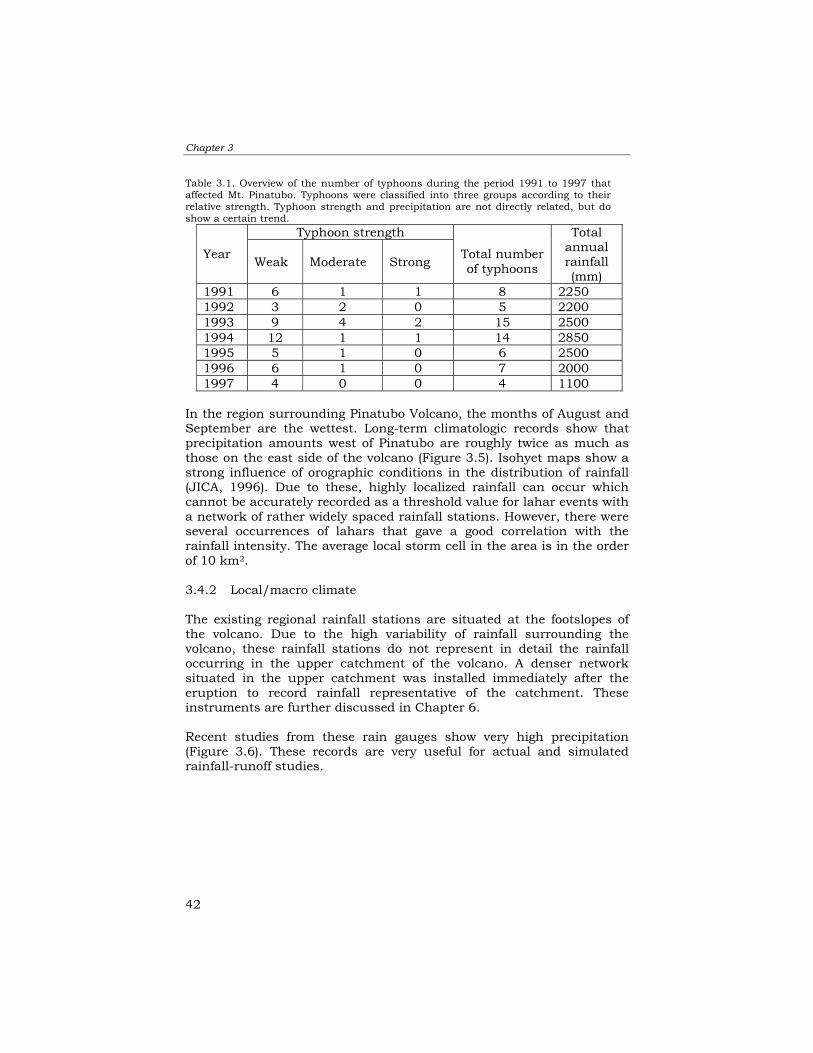
Chapter 3
42
Table 3.1. Overview of the number of typhoons during the period 1991 to 1997 that affected Mt. Pinatubo. Typhoons were classified into three groups according to their relative strength. Typhoon strength and precipitation are not directly related, but do show a certain trend.
Typhoon strength
Year Weak Moderate Strong
Total number of typhoons
Total annual rainfall (mm)
1991 6 1 1 8 2250 1992 3 2 0 5 2200 1993 9 4 2 15 2500 1994 12 1 1 14 2850 1995 5 1 0 6 2500 1996 6 1 0 7 2000 1997 4 0 0 4 1100
In the region surrounding Pinatubo Volcano, the months of August and September are the wettest. Long-term climatologic records show that precipitation amounts west of Pinatubo are roughly twice as much as those on the east side of the volcano (Figure 3.5). Isohyet maps show a strong influence of orographic conditions in the distribution of rainfall (JICA, 1996). Due to these, highly localized rainfall can occur which cannot be accurately recorded as a threshold value for lahar events with a network of rather widely spaced rainfall stations. However, there were several occurrences of lahars that gave a good correlation with the rainfall intensity. The average local storm cell in the area is in the order of 10 km2. 3.4.2 Local/macro climate The existing regional rainfall stations are situated at the footslopes of the volcano. Due to the high variability of rainfall surrounding the volcano, these rainfall stations do not represent in detail the rainfall occurring in the upper catchment of the volcano. A denser network situated in the upper catchment was installed immediately after the eruption to record rainfall representative of the catchment. These instruments are further discussed in Chapter 6. Recent studies from these rain gauges show very high precipitation (Figure 3.6). These records are very useful for actual and simulated rainfall-runoff studies.
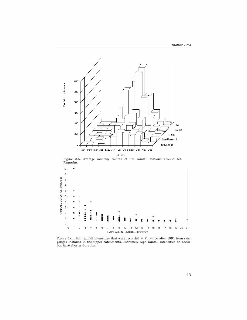
Pinatubo Area
43
OCCURRENCES OF HIGH RAINFALL INTENSITIES (>0.5mm/min) RECORDED BY RAIN GAUGES IN THE VICINITY OF PASIG WATERSHED
0
1
2
3
4
5
6
7
8
9
10
0 1 2 3 4 5 6 7 8 9 10 11 12 13 14 15 16 17 18 19 20 21RAINFALL INTENSITIES (mm/min)
RAI
NFA
LL D
UR
ATIO
N (m
inut
es)
Figure 3.6. High rainfall intensities that were recorded at Pinatubo after 1991 from raingauges installed in the upper catchments. Extremely high rainfall intensities do occurbut have shorter duration.
Figure 3.5. Average monthly rainfall of five rainfall stations around Mt.Pinatubo.
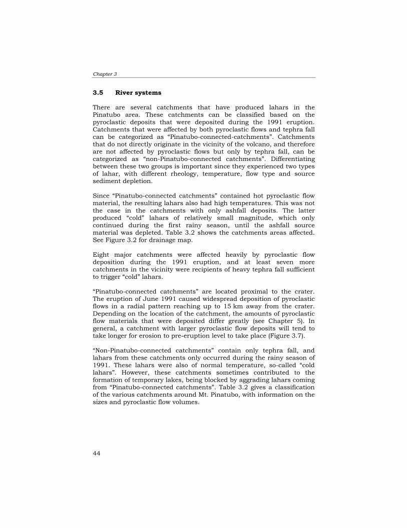
Chapter 3
44
3.5 River systems There are several catchments that have produced lahars in the Pinatubo area. These catchments can be classified based on the pyroclastic deposits that were deposited during the 1991 eruption. Catchments that were affected by both pyroclastic flows and tephra fall can be categorized as “Pinatubo-connected-catchments”. Catchments that do not directly originate in the vicinity of the volcano, and therefore are not affected by pyroclastic flows but only by tephra fall, can be categorized as “non-Pinatubo-connected catchments”. Differentiating between these two groups is important since they experienced two types of lahar, with different rheology, temperature, flow type and source sediment depletion. Since “Pinatubo-connected catchments” contained hot pyroclastic flow material, the resulting lahars also had high temperatures. This was not the case in the catchments with only ashfall deposits. The latter produced “cold” lahars of relatively small magnitude, which only continued during the first rainy season, until the ashfall source material was depleted. Table 3.2 shows the catchments areas affected. See Figure 3.2 for drainage map. Eight major catchments were affected heavily by pyroclastic flow deposition during the 1991 eruption, and at least seven more catchments in the vicinity were recipients of heavy tephra fall sufficient to trigger “cold” lahars. “Pinatubo-connected catchments” are located proximal to the crater. The eruption of June 1991 caused widespread deposition of pyroclastic flows in a radial pattern reaching up to 15 km away from the crater. Depending on the location of the catchment, the amounts of pyroclastic flow materials that were deposited differ greatly (see Chapter 5). In general, a catchment with larger pyroclastic flow deposits will tend to take longer for erosion to pre-eruption level to take place (Figure 3.7). “Non-Pinatubo-connected catchments” contain only tephra fall, and lahars from these catchments only occurred during the rainy season of 1991. These lahars were also of normal temperature, so-called “cold lahars”. However, these catchments sometimes contributed to the formation of temporary lakes, being blocked by aggrading lahars coming from “Pinatubo-connected catchments”. Table 3.2 gives a classification of the various catchments around Mt. Pinatubo, with information on the sizes and pyroclastic flow volumes.
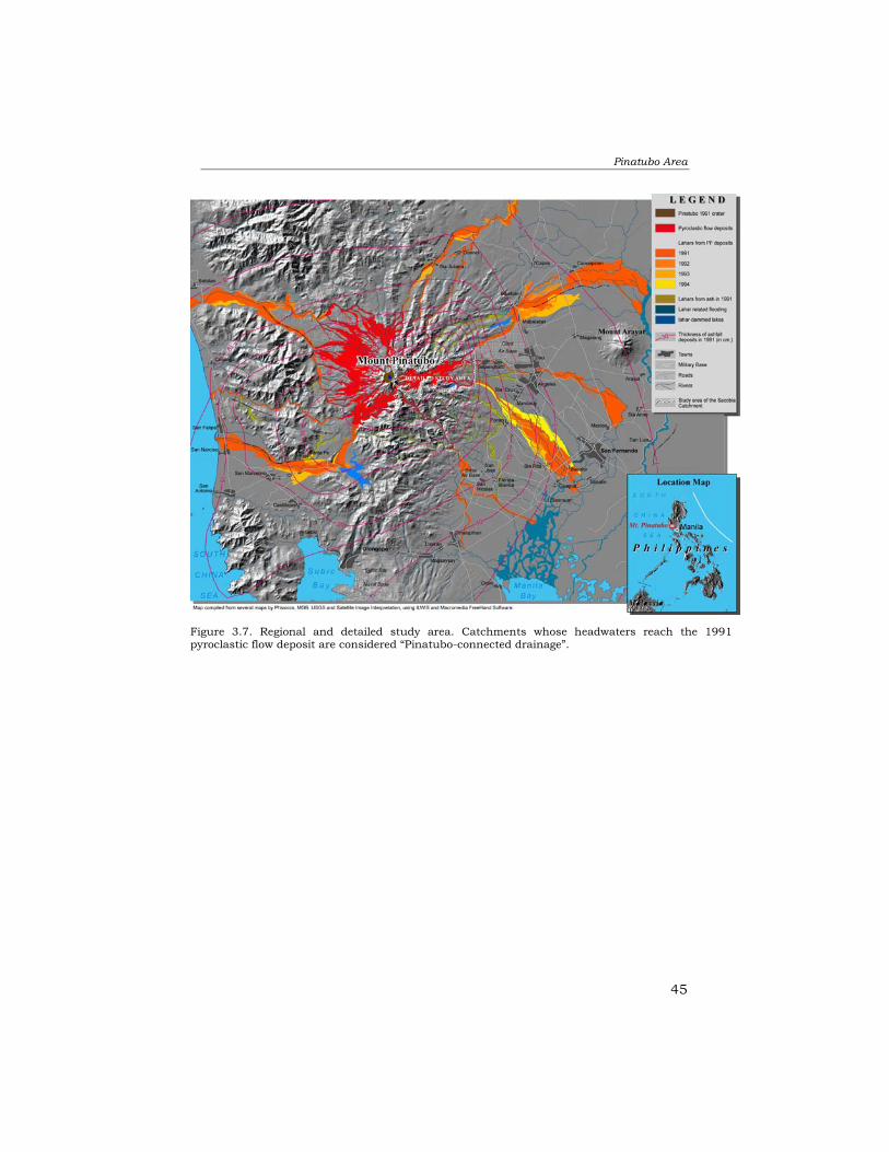
Pinatubo Area
45
Figure 3.7. Regional and detailed study area. Catchments whose headwaters reach the 1991pyroclastic flow deposit are considered “Pinatubo-connected drainage”.

Chapter 3
46
Table 3.2. List of catchments classified as “Pinatubo-catchment” and “non-Pinatubo catchment” (see figure 3.2 for reference).
Catchment Area (km2) VOLUME of pyroclastic flows (km3)
PINATUBO-connected catchment O’Donnel 89 0.6 Sacobia Pasig Abacan
64 1.28
Marella 79 1.3 Bucao 262 3.1 Gumain 41 Porac 81 0.06
NON-PINATUBO-connected catchment Taug 6.6 Tanguay 77 Balintawak 175 Maloma 153 Kileng 41 Cauayan Marimla 70 Bangat 80
If we consider the effects in the distal reaches of the catchments of Mt. Pinatubo, it can be concluded that the large sediment supply has led to sedimentation problems far away from the volcano. Sedimentation problems were reported as far as 30 km to the west, into the China Sea; about 100 km to the north, reaching the Lingayen Gulf; 70 km east, affecting the Candaba Swamp; and 40 km to the south, all the way to Pampanga Bay. The total influence of its siltation encompasses the provinces of Bulacan, Nueva Ecija, Pangasinan and Bataan. 3.6 Pre-eruption land-use situation Dense forest covered the upper slopes of the volcanic centers around Mt. Pinatubo prior to the eruption. The upper slopes were being used for jungle survival training for US military personnel conducted by the Aetas (native highlanders). In the upper portions, the natives use shifting cultivation because of the low soil fertility. There were only a limited number of isolated inhabitants on these upper slopes. The Aetas had a population of about 20,000 and they dominate on the upper slopes. One of the important projects that was undertaken in the area prior to eruption was the unsuccessful geothermal exploration conducted by the Philippine National Oil Company. Three exploration drilling wells were sunk from 1988 to 1990, with depths from 2.1 to 2.7 km and with

Pinatubo Area
47
subsurface temperatures from 261° to 336°C. However, due to the acidic nature of the Na-Cl waters in the well (pH=2.3-4.3), the project was abandoned (Delfin et al.,1996). On the lower slopes, where lahar deposits dominated the area, the main agricultural crops were sugar cane and vegetables. Extensive areas with cogon grasses could be found on idle lands. Aquaculture farming was practiced especially on areas with a shallow water table. There were a large number of fast-growing villages and cities, especially on the eastern side of the volcano. Angeles City is the most densely populated area and is situated only about 20 km downslope. There were three military facilities at the foot of the volcano, namely Subic Naval Base, Clark Air force Base and Basa Air force Base. The first two belonged to the American Armed Forces and housed a large number of personnel (about 25,000 including family members) and were both located near to major cities, namely Olongapo and Angeles City (see Figure 3.7). 3.7 Study area In this research different scales of analysis have been used at Mt. Pinatubo, depending on the type of investigation. A regional-scale study was done using several remote sensing data. These cover an area of about 60 x 60 km centered at Mt. Pinatubo crater. At this scale, the types of study conducted were: change detection of land cover, vegetation, pyroclastic flow and lahar deposits. Large-scale studies were done in the Sacobia-Pasig-Abacan catchments located at the east side of the volcano (see Figure 3.7). The total upper catchment area is about 64 km2 with an estimated pyroclastic flow volume of 1.3 km3. Although these catchments have a smaller volume of pyroclastic flow deposits as compared with the western side, the downstream portions are heavily populated and highly developed in the region. Most investigations reported here were done in this area.

Chapter 3
48

Monitoring the 1991 Eruption & Post-eruption Using R.S. Images
49
Chapter 4 : Monitoring the 1991 Eruption and Post-eruption Using Remote Sensing Images 4.1 Introduction The aftermath of the 15-16 June 1991 climactic eruption resulted in the rapid erosion of fresh pyroclastic flow deposits and numerous lahars. The eruption affected eight major catchments surrounding the volcano and the volume of the new pyroclastic flow deposits from the eruption was estimated to be in the order of 5.5 to 7 billion cubic meters (Daligdig et al., 1992; Scott et al., 1996). About 75% of these deposits were accumulated in the western catchments, which are less inhabited than those on the eastern side. The volume of the 1991 Mt. Pinatubo pyroclastic flows was so large that several drainage divides were buried, resulting in a dramatic change in catchment boundaries. These changes had strong implications for the rate of erosion and the areas affected by lahars. The presence of hot fine-sand-dominated pyroclastic flow deposits in the upper catchments resulted in large erosion volumes and associated lahars, even with slight to moderate rainfall. 4.2 Eruption chronology and deposits The climax of the 1991 eruption started at 13:42 hrs on 15 June, when continuous high-amplitude tremors began to saturate all operating seismographs. By 14:30 hrs all telemetered seismographs located on the upper slopes within 10 km of the volcano suddenly became inoperative, leaving only the seismograph located at Clark Air Base operational, a distance of 25 km away from the crater. It was concluded that the other seismographs had been hit by cascading pyroclastic flows or by large volumes of volcanic ash. Pumiceous ashfall as large as 4 cm in diameter were experienced at Clark Air Base Volcano Observatory. By this time, the monitoring team decided to evacuate the post due to the imminent threat of eruption, since the observatory lies within the fringes of the pre-1991 pyroclastic flow deposits. Likewise, visibility was less than a few meters due to continuous ashfall. The situation deteriorated continuously for several hours until the early morning of 16 June. During this period, earthquakes were experienced almost every minute at the evacuation camp located 38 km east of the volcano. Based on instrumental records, the peak of the eruption lasted from 13:42 hrs until 22:30 hrs on 15 June (Wolf and Hoblitt, 1996). It was implied that this was the period of emplacement of the voluminous
Chapter 4
50
pyroclastic flows and the subsequent destruction and collapse of Pinatubo’s summit into a 2.5 km wide caldera. Pyroclastic flow deposits and ashfall deposits (Figures 4.1 and 4.2) from the climactic eruption have been extensively studied and described (Scott et al., 1996; Paladio et al., 1996). The estimated magma volume was in the order of 3.7 to 5.3 km3 and when ejected it would have an estimated volume of about 8.4 to 10.4 km3 of porous pumiceous tephra and pyroclastic flow deposits (Scott et al., 1996). The pyroclastic flows devastated an area of more than 400 km2 and fine ash blanketed several countries in Southeast Asia (Paladio et al., 1996). 4.2.1 Tephra from the climactic eruption A study on the initiation and duration of tephra fall from the climactic eruption was based on seismic data, barograph measurements, visual observations and the use of satellites. During the peak of the eruption, visual observation was impossible since visibility was only a few meters. The eruption column reached an altitude of at least 35 km, spreading broadly in the stratosphere and eventually reaching a distance of 250 km upwind in the northeastern direction (Koyaguchi, 1996). An area of about 7,500 km2 on the island of Luzon was covered by more than 1 cm of tephra and almost the entire island, with an area of 105,000 km2, received at least a trace (Paladio et al., 1996). Wiesner and Wang (1996) reconstructed the westerly elongated ash cloud reflecting the direction of upper-level winds, as evidenced by the tephra collected from sea bottom cores with traces of ashfall in the South China Sea, extending from 10° to 16°N and 111° to 120°E. The total bulk volume of the airfall ash is calculated at 2.7 km3, including the volume of 0.9 km3 of ash that was deposited in the South China Sea (Wiesner and Wang, 1996). The atmospheric spread of the ash clouds was monitored using NOAA AVHRR and the Japanese GMS meteorological satellite images (Self et al., 1996; Lynch and Stephens, 1996). From these images a thick umbrella cloud of at least 100 km radius could be seen spreading out (Figure 4.3). By the next day, 16 June, traces of ash blanketed several Southeast Asian countries (Figure 4.4). Thirty-six hours after the climactic eruption, an area of approximately 2,700,000 km2 was affected by ashfall, including countries such as Thailand, Cambodia, Vietnam and Singapore (Lynch and Stephens, 1996). Ashfall distribution on Luzon within a radius of 60 km from the volcano was mapped by Paladio et al. (1996). They estimated an ash volume within this area of about 1.7 km3, with a maximum thickness of 39 cm
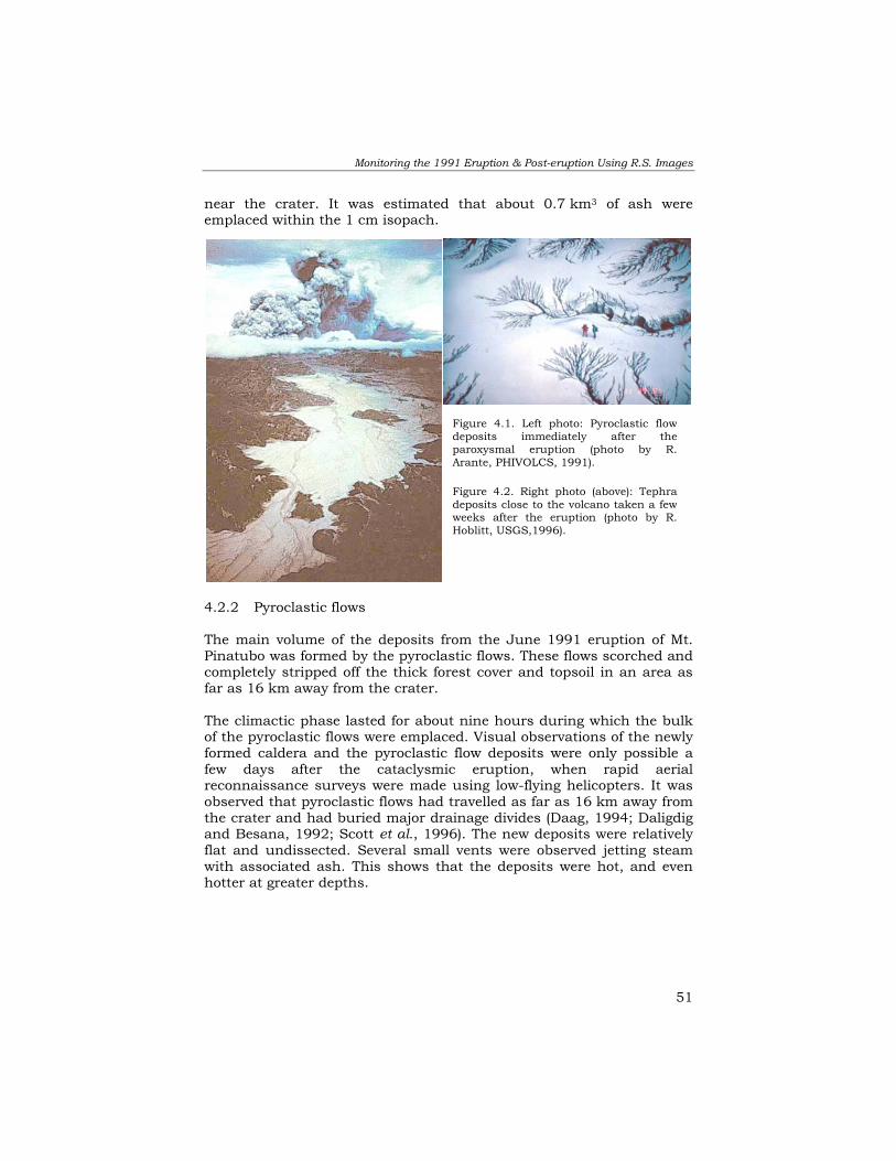
Monitoring the 1991 Eruption & Post-eruption Using R.S. Images
51
near the crater. It was estimated that about 0.7 km3 of ash were emplaced within the 1 cm isopach.
4.2.2 Pyroclastic flows The main volume of the deposits from the June 1991 eruption of Mt. Pinatubo was formed by the pyroclastic flows. These flows scorched and completely stripped off the thick forest cover and topsoil in an area as far as 16 km away from the crater. The climactic phase lasted for about nine hours during which the bulk of the pyroclastic flows were emplaced. Visual observations of the newly formed caldera and the pyroclastic flow deposits were only possible a few days after the cataclysmic eruption, when rapid aerial reconnaissance surveys were made using low-flying helicopters. It was observed that pyroclastic flows had travelled as far as 16 km away from the crater and had buried major drainage divides (Daag, 1994; Daligdig and Besana, 1992; Scott et al., 1996). The new deposits were relatively flat and undissected. Several small vents were observed jetting steam with associated ash. This shows that the deposits were hot, and even hotter at greater depths.
Figure 4.1. Left photo: Pyroclastic flowdeposits immediately after theparoxysmal eruption (photo by R.Arante, PHIVOLCS, 1991). Figure 4.2. Right photo (above): Tephradeposits close to the volcano taken a fewweeks after the eruption (photo by R.Hoblitt, USGS,1996).

Chapter 4
52
Surface measurements of distal pyroclastic flows (16 km from the crater) taken several weeks after the eruption revealed an average temperature of 220°C at a depth of half a meter. The pyroclastic flow deposits are poor conductors of heat, and their inherent heat will
dissipate over a longer time period, especially at greater depths. This was proven by a series of steam explosions observed along a newly exposed channel even after five years of emplacement (PHIVOLCS Pinatubo Bulletins, 1991-1995). In order to map the situation after the eruption, a series of oblique aerial photographs were taken from low-flying helicopters. They were also used for the volumetric calculation of pyroclastic flow deposits by reconstructing the valley-fill cross-section (see Chapter 5). Total volumes of pyroclastic flows in all catchments were estimated between 5.5 and 7 km3 Daligdig and Besana, 1992; USACE, 1996; Punongbayan et al., 1996; Scott et al., 1996).
Figure 4.3. Sequence of GMS images (visible and thermal infrared bands) of the Pinatuboash cloud that developed in three hours, from 13:40 to 16:40 hrs, on 15 June 1991 (afterSelf et al., 1996).

Monitoring the 1991 Eruption & Post-eruption Using R.S. Images
53
Scott et al. (1996) made detailed stratigraphic studies of the 1991 pyroclastic flow deposits and distinguished three facies. The first consists of the massive pumiceous deposits that form the valley fills and fans, and is by far the most voluminous and extensive. The maximum thickness of these deposits was determined to be about 100 m. The second facies consists of stratified pumiceous pyroclastic flow deposits that covered the medial part of the catchment and contains numerous layers several centimetres thick, but with a total thickness not exceeding 5 m. The third is the prominent lithic-rich facies that also rarely exceeds 5 m, consisting of clast-supported layers from the former Pinatubo’s summit dome. This deposit is found within 5 km of the crater. Figure 4.5 shows the spatial distribution of the three pyroclastic flow facies. Field observations showed that the pyroclastic flow deposits in dry condition were friable, non-welded, very loose and non-cohesive. The bulk densities of the pyroclastic flow materials were in the order of 1.0 to 1.3 g/cm3 (Scott et al., 1996). There was little or no evidence of contacts separating different flow units in many massive pyroclastic flows, even with a total thickness ranging up to tens of meters (Figure 4.5). This massive deposit consists for 70 to 85% of sands. Coarser fragments constitute no more than 5 to 20% and fine ash (finer than 0.0625 mm) accounts for a maximum of 18% in weight (Scott et al., 1996).
Figure 4.4. Movement of ash cloud reported at three-hour intervals(source: Self et al., 1996).
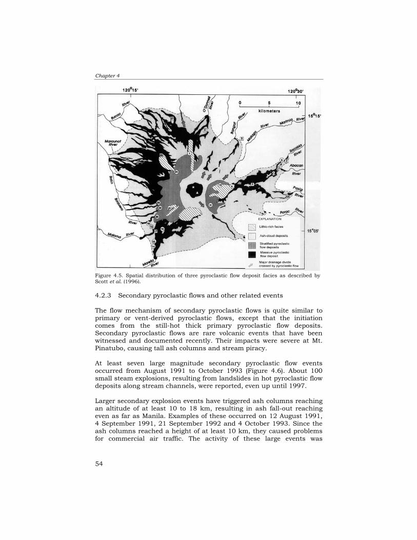
Chapter 4
54
4.2.3 Secondary pyroclastic flows and other related events The flow mechanism of secondary pyroclastic flows is quite similar to primary or vent-derived pyroclastic flows, except that the initiation comes from the still-hot thick primary pyroclastic flow deposits. Secondary pyroclastic flows are rare volcanic events that have been witnessed and documented recently. Their impacts were severe at Mt. Pinatubo, causing tall ash columns and stream piracy. At least seven large magnitude secondary pyroclastic flow events occurred from August 1991 to October 1993 (Figure 4.6). About 100 small steam explosions, resulting from landslides in hot pyroclastic flow deposits along stream channels, were reported, even up until 1997. Larger secondary explosion events have triggered ash columns reaching an altitude of at least 10 to 18 km, resulting in ash fall-out reaching even as far as Manila. Examples of these occurred on 12 August 1991, 4 September 1991, 21 September 1992 and 4 October 1993. Since the ash columns reached a height of at least 10 km, they caused problems for commercial air traffic. The activity of these large events was
Figure 4.5. Spatial distribution of three pyroclastic flow deposit facies as described byScott et al. (1996).

Monitoring the 1991 Eruption & Post-eruption Using R.S. Images
55
monitored by seismographs since their mechanism involved continuous avalanching and subsequent flows yielding localized vibrations. Seismographs located several kilometres from the site of explosion were able to record the activity. Heights of the ash columns produced were monitored using ground-based radar.
Secondary pyroclastic flow events can leave geomorphologic evidence, which is recognizable on aerial photographs or satellite images, in the form of avalanche crowns or shallow “amphitheatre” forms that are in the order of a few tens of meters deep and about 1 km wide (Figure 4.7). The resulting secondary pyroclastic flows can reach a few kilometres downslope, leaving distinct smooth undissected lobes of flow deposits that can be clearly distinguished from the more dissected older pyroclastic flow deposits (Figure 4.8). Field observations revealed that secondary pyroclastic flow deposits showed sedimentologic structures similar to those of the primary pyroclastic flow deposits, which made it quite difficult to distinguish both types of deposits. Torres et al. (1996) found differences only in the
Figure 4.6. Map showing the locations of secondary pyroclastic flows on the1991 pyroclastic flow deposits (Torres et al., 1996).

Chapter 4
56
percentage of fines present in the two types of deposits. Secondary pyroclastic flow deposits were found to have a few percent less fines, which is due to the release of fine ash by elutriations during the flow. No new fragmentation has occurred since their mobility has become slower. One method of distinguishing between the two types of deposits is by determining the magnetic orientation of the clasts. The clasts from secondary pyroclastic flows have a random orientation, as opposed to the more preferred orientation of the primary pyroclastic flow deposits. This reveals that the secondary pyroclastic flows were emplaced with a colder temperature, at least below the melting point (Curie temperature) of magnetite, thus justifying their random orientation.
The secondary pyroclastic flows can travel as much as 8 km downstream and can have a volume of about 0.01 to 0.05 km3, sometimes leaving a crater of about 2 km2. Since their volume is relatively small, most of their deposits are channel-confined. The impact of secondary pyroclastic flows can be devastating. Apart from the hazards caused by ash columns and the redeposition of hot ash flows, they may also lead to stream piracy. Such stream piracies have been documented twice in the Sacobia catchment. One of these occurred on 4 April 1992 and led to the capture of the Abacan catchment by the Sacobia River. The other happened on 4 October 1993, during which the upper Sacobia catchment was captured by the Pasig River. 4.3 Monitoring changes Eight optical satellite images were available for this study in order to monitor the surface changes from 1988 to 2000 at a synoptic scale. The optical sensors used were:
Figure 4.7. Secondary explosion crater thatoccurred in the upper Abacan River.
Figure 4.8. Newly emplaced secondarypyroclastic flow deposit in the Sacobiachannel, which occurred on 4 April1992.

Monitoring the 1991 Eruption & Post-eruption Using R.S. Images
57
• SPOT Multispectral. Spectral bands are: near-infrared (0.79-0.89 µm), red (0.61-0.68 µm), and green (0.50-0.59 µm). Ground resolution is 20 m.
• Landsat Thematic Mapper. Spectral bands are: visible (Band 1 = 0.45-0.52 µm, Band 2 = 0.52-0.60 µm, and Band 3 = 0.63-0.69 µm); near-infrared (Band 4 = 0.76-0.90 µm); SWIR (short-wave infrared) band (Band 5 = 1.55-1.75 µm, Band 6 = 10.40-12.50 µm, and Band 7 = 2.08-2.35 µm). Ground resolutions are 30 m, except Band 6, which is 120 m.
To monitor and quantify the changes at a more detailed scale, four sets of vertical aerial photographs were used to study the upper Sacobia-Pasig-Abacan catchment. The following images were used. Optical satellite images: • 4 February 1988: SPOT multispectral • 18 December 1991: SPOT multispecral • 26 January 1992: Landsat TM • 25 April 1995: SPOT multispectral • 11 December 1997: SPOT multispectral • 16 January 2000: Landsat TM Vertical panchromatic aerial photographs: • 1:15,000: Nov 1991 • 1:25,000: Oct 1992 • 1:15,000: Mar 1994 • 1:15,000: Feb 1996 4.3.1 Changes due to deposition and erosion The satellite images presented in Figure 4.9 were processed using standard false colour composites in order to map the distribution of the pyroclastic flow deposits, the vegetation cover and the lahar deposits for several time intervals. Band combinations for SPOT images are Band 3 for red, Band 2 for green, and Band 1 for blue. For TM images, the combinations are Band 4 for red, Band 3 for green and Band 2 for blue. The original scenes (full scene) were initially used, which makes the areas covered per scene little different. SPOT and Landsat images have different pixel resolutions. The Landsat data were georeferenced with the SPOT 1988, using image-to-image georeferencing. Later, in the analysis of NDVI and image classification, a mask was used to exclude areas that were not common. The 1988 (pre-eruption) image indicates that most of Mt. Pinatubo and the surrounding areas have a dense

Chapter 4
58
vegetation cover, with tropical forest on the upper slopes. The areas with dense vegetation cover largely consist of old pyroclastic flow deposits. At the distal part of the volcano, there are sand-rich deposits, identified in the image by their bluish colour, which are actually old lahar deposits. The pyroclastic flows from the eruption in 1991 completely stripped off the thick forest cover on the upper slopes and left the area completely bare, affecting 400 km2 (Scott et al., 1996). The December 1991 image was taken after the first rainy season following the eruption. A crater measuring 2.5 km in diameter developed as a result of summit collapse. Extensive tephra fall mantled the surrounding slopes, which appear like snow-capped mountains. Several lahar fans developed at the footslopes of the volcano, reaching up to 40 km. The image from 1991 clearly shows that the lateral deposition of lahar was more active on the east side of the volcano, because the channels are much shallower, leading to frequent avulsion during lahar events. Although the lahar magnitude on the western side was much greater, the area covered by lahars was relatively smaller, due to the deeper valleys and fewer avulsion phenomena. One other noticeable feature in the images is the rapid decrease in ashfall cover, which was almost completely eroded within a time span of two years. The 1991 and 1992 images show clear signs of thick ashfall deposits, which are especially prominent on the western part of the volcano, where the thickness of ashfall was greater. Images taken in 1995, 1997 and 2000 show few remains of ashfall deposits, and show that vegetation has recovered in most of the ashfall-affected areas. There were significant changes in the lahar delivery after the October 1994 capture of the upper Sacobia catchment by the Pasig River. Figures 4.10 and 4.11 show a significant increase in the lahar deposits downstream of the Pasig River. Due to the increased size of the Pasig catchment, after the stream piracy (section 4.4.3), a large part of the pyroclastic flow deposit of the upper catchment was transported by the Pasig River, and the downstream section experienced a drastic increase in the magnitude of lahar flows. Likewise, there was an increase in channel width due to extensive lateral erosion. Due to the great change in lahar volumes, numerous avulsions took place from the Pasig channel. The dike shown in 1992 (Figure 4.12) clearly did not have sufficient capacity to contain the increased lahar volumes. Therefore a “megadike” more than 50 km long was constructed in 1995 in order to contain the lahars (Figure 4.13).

Monitoring the 1991 Eruption & Post-eruption Using R.S. Images
59
4.3.2 Land cover changes In order to assess the large-scale changes of Mt. Pinatubo on a regional scale, the available satellite images were processed using a supervised maximum likelihood classification. The maximum likelihood classification assumes that spectral values of training pixels are statistically distributed according to a "multi-variate normal probability density function" (Lillesand and Kiefer, 2000). For each set of spectral input values, the distance towards each of the classes was calculated using the so-called Mahalanobis distance. The class name with the shortest distance is assigned if this distance is smaller than the user-defined threshold value (ILWIS, 1997). Figure 4.14 shows an example of the sample set obtained from the 1991 SPOT image. Land cover classes are pyroclastic flow deposit, ashfall, water/lake or sea, vegetation, wet lahar, dry lahar and clouds. Spectral mixing is very high for pyroclastic flow deposits and dry lahar. This was also recognized by other researchers who worked in the area, such as Atienza (1995), Calomarde (1997) and Castro (1999).
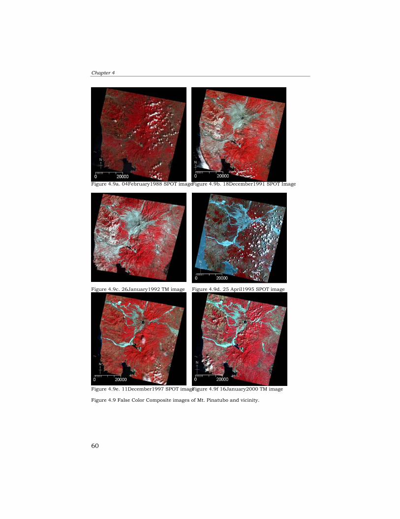
Chapter 4
60
Figure 4.9 False Color Composite images of Mt. Pinatubo and vicinity.
Figure 4.9a. 04February1988 SPOT imageFigure 4.9b. 18December1991 SPOT Image
Figure 4.9c. 26January1992 TM image Figure 4.9d. 25 April1995 SPOT image
Figure 4.9e. 11December1997 SPOT imageFigure 4.9f 16January2000 TM image

Monitoring the 1991 Eruption & Post-eruption Using R.S. Images
61
Figure 4.10. 26 January 1992 Landsat TM image of lower Pasig River.
Figure 4.11. 11 December 1997 SPOT image of lower Pasig River.

Chapter 4
62
Figure 4.12. 26 January 1992 Landsat TM image showing the lower reachesof the Pasig River.
Figure 4.13. 16 January 2000 Landsat TM image showing the construction ofdike system.

Monitoring the 1991 Eruption & Post-eruption Using R.S. Images
63
The DN values of vegetation, water body and wet lahars can be classified easily. Knowledge-based post-classification of pyroclastic flows and dry lahar improved the land cover map (Table 4.1).
Figure 4.14 shows the results of the supervised classification. The different figures show the pyroclastic flow deposits of the 1991 eruption in red, the development of lakes in blue, and lahars in orange and yellow. Wet and dry lahars show significant spectral differences and can be classified separately. It can be noticed that the 1 April 1988 image shows significant sandy lahars in major drainages, even before the eruption. This would mean that deposition of sandy materials is high. Several lakes have evolved in the vicinity of the volcano. As mentioned in Chapter 2, their development is generally attributable to lahar aggradation or the damming of non-Pinatubo-connected catchments. The most prominent lakes that developed are the Mapanuepe Lake and the Mt. Cutuno Lake in Pasig, located on the southwest and east parts of the volcano, respectively. The crater lake has increased significantly; likewise dome growth has evolved since 1992 (Daag et al., 1996). Table 4.1 shows the result of changes in land cover area. Each year (except for 1988) pre-classification and post-classification values are shown in order to distinguish the improvement in the classifications. Significant changes can be quantified and the growth of vegetation is
Figure 4.14. Sample set ofSPOT 1991 used in thesupervised classification.Note that spectral mixing isevident on the pyroclasticflow deposit and dry lahar.Post-classification wasdone to improve the landcover map.

Chapter 4
64
among the most observable changes. The eruption in 1991 reduced the vegetation cover by about 132 km2, mainly due to the deposition of pyroclastic flow deposits and ashfall. Vegetation has increased, even partially on the 1991 pyroclastic flow deposits. However, some variations in the vegetation cover are affected by seasonal changes caused by the weather. The presence of pyroclastic flows is noticeable in the different images after the eruption. Table 4.1. Land cover map changes as monitored by using satellite images. Knowledge-based pre- and post-classifications were done on most images in order to improve the classification. Values are in km2.
1988 1991 1992 1995 1997 2000
pre post pre post pre post pre post pre post
Wet Lahar 69 69 97 97 44 44 36 36 50 50
Dry Lahar 297 63 121 291 314 2 457 63 246 74 381 Pyroclastic Flow 190 132 97 74 637 181 290 107 405 99
Water Body 127 115 115 119 119 123 123 143 143 138 138
Vegetation 2,267 2,250 2,250 2,383 2,383 2,181 2,181 2,454 2,454 2,319 2,319
Ashfall 73 73
Clouds 295 226 226
Total 2,987 2,987 2,987 2,987 2,987 2,987 2,987 2,987 2,987 2,987 2,987
4.3.3 Vegetation changes Vegetation growth can be excellently monitored using multi-spectral satellite images, due to the presence of infrared bands that are sensitive to vegetation. A standard way to monitor vegetation changes is through the use of a Normalized Difference Vegetation Index (NDVI). NDVI values range from -1 to 1. In principle, vegetated areas will generally yield high values because of their relatively high near-infrared reflectance and relatively low visible reflectance. In contrast, water and clouds have greater visible reflectance than near-infrared reflectance. Thus, these features yield negative index values. Rock, bare soil, pyroclastic flows and lahar areas have similar reflectance in the two bands and result in vegetation indices near zero (ILWIS Manual, 1997; Chen 1988a and 1988b).
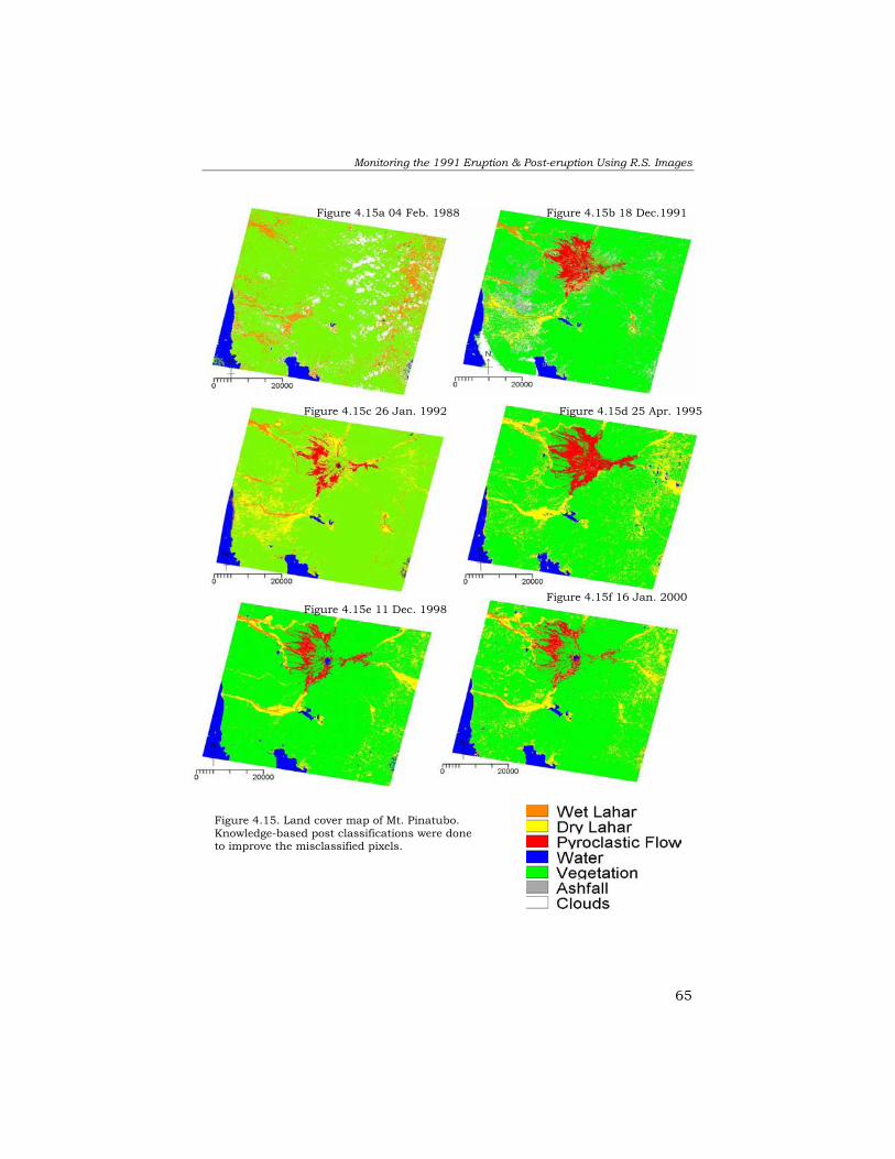
Monitoring the 1991 Eruption & Post-eruption Using R.S. Images
65
Figure 4.15. Land cover map of Mt. Pinatubo. Knowledge-based post classifications were doneto improve the misclassified pixels.
Figure 4.15b 18 Dec.1991Figure 4.15a 04 Feb. 1988
Figure 4.15c 26 Jan. 1992 Figure 4.15d 25 Apr. 1995
Figure 4.15f 16 Jan. 2000Figure 4.15e 11 Dec. 1998

Chapter 4
66
For all the available images NDVI maps were generated (see Figure 4.16). All images were normalized using histogram equalization before calculating the NDVI. The images show the distribution and intensity of vegetation growth through time. Compared with the 1988 image, the one of 1991 shows a large decrease in vegetation over several hundreds of square kilometres. There were no clear signs of regeneration of vegetation in areas that were directly affected by pyroclastic flows. The 1991 map shows only high NDVI values for those areas that were only affected by ashfall, indicating that most ash material was already removed from the vegetation by the end of the first rainy season following the eruption. Selective vegetation growth on the new deposits began to appear around 1994 but was mostly limited to cogon grasses (a tall grass variety that can survive on soils with minimal nutrients). In the upper catchment, the vegetation growth occurs only in areas with pre-1991 pyroclastic flows and other older deposits, but never on the 1991 pyroclastic flows and lahars. Thus, with these conditions, it is possible to distinguish the 1991 deposits from the pre-1991 by looking at the vegetation growth. The maps of 1995, 1997 and 2000 display a progressive growth of vegetation. In most cases, vegetation is denser in areas with exposed pre-1991 eruption deposits. Table 4.2 shows the NDVI changes as percentages. An increase in vegetation cover is noticeable in the images of years 1995, 1997 and 2000. Table 4.2. Distribution of NDVI values per area coverage in percent.
NDVI range
SPOT 1988
SPOT 1991
TM 1992
SPOT 1995
SPOT 1997
TM 2000
-1 0.07 0.83 -0.8 0.00 2.13 0.00 -0.6 0.00 1.22 2.64 -0.4 0.00 3.62 25.51 0.00 0.01 -0.2 4.53 24.22 30.65 5.01 9.75 8.51
0 51.19 44.51 28.94 51.93 42.65 36.21 0.2 37.06 21.89 12.08 35.26 39.64 49.57 0.4 7.02 1.23 0.17 7.57 7.96 5.71 0.6 0.22 0.00 0.8 1 0.12 0.35

Monitoring the 1991 Eruption & Post-eruption Using R.S. Images
67
Fig.4.16a. Feb 4,1988 Fig. 4.16b. Dec 18,1991
Fig. 4.16d. 25 Apr. 1995 Fig. 4.16c. 26 Jan.1992
Figure 4.16. Derived NDVI values of different satellite images.
1.000.670.330.00-0.33-0.67-1.00
Fig. 4.16e. 11 Dec.1997 Fig. 4.16f. 16 Jan. 2000
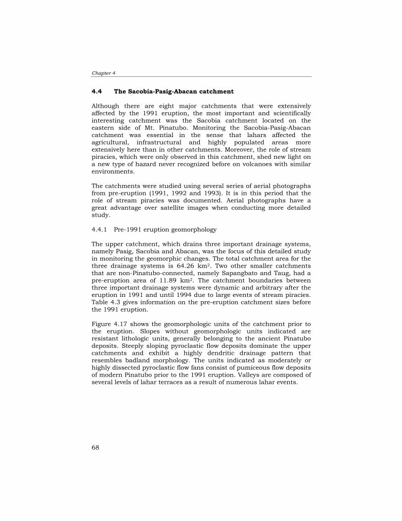
Chapter 4
68
4.4 The Sacobia-Pasig-Abacan catchment Although there are eight major catchments that were extensively affected by the 1991 eruption, the most important and scientifically interesting catchment was the Sacobia catchment located on the eastern side of Mt. Pinatubo. Monitoring the Sacobia-Pasig-Abacan catchment was essential in the sense that lahars affected the agricultural, infrastructural and highly populated areas more extensively here than in other catchments. Moreover, the role of stream piracies, which were only observed in this catchment, shed new light on a new type of hazard never recognized before on volcanoes with similar environments. The catchments were studied using several series of aerial photographs from pre-eruption (1991, 1992 and 1993). It is in this period that the role of stream piracies was documented. Aerial photographs have a great advantage over satellite images when conducting more detailed study. 4.4.1 Pre-1991 eruption geomorphology The upper catchment, which drains three important drainage systems, namely Pasig, Sacobia and Abacan, was the focus of this detailed study in monitoring the geomorphic changes. The total catchment area for the three drainage systems is 64.26 km2. Two other smaller catchments that are non-Pinatubo-connected, namely Sapangbato and Taug, had a pre-eruption area of 11.89 km2. The catchment boundaries between three important drainage systems were dynamic and arbitrary after the eruption in 1991 and until 1994 due to large events of stream piracies. Table 4.3 gives information on the pre-eruption catchment sizes before the 1991 eruption. Figure 4.17 shows the geomorphologic units of the catchment prior to the eruption. Slopes without geomorphologic units indicated are resistant lithologic units, generally belonging to the ancient Pinatubo deposits. Steeply sloping pyroclastic flow deposits dominate the upper catchments and exhibit a highly dendritic drainage pattern that resembles badland morphology. The units indicated as moderately or highly dissected pyroclastic flow fans consist of pumiceous flow deposits of modern Pinatubo prior to the 1991 eruption. Valleys are composed of several levels of lahar terraces as a result of numerous lahar events.

Monitoring the 1991 Eruption & Post-eruption Using R.S. Images
69
Table 4.3. Pre-eruption catchment sizes and volumes of 1991 pyroclastic flows.
Catchment Catchment Area (km2)
Sacobia North Upper Sacobia South Upper Sacobia Lower Sacobia
39.82 9.97 11.73 18.12
Pasig Bucbuc Papatak Timbu Yanca
21.90 5.95 6.46 4.94 4.55
Abacan 2.54 SapangBato 5.29 Taug 6.60
4.4.2 Post-eruption geomorphology The post-eruption geomorphology describes the terrain conditions immediately after the eruption, when significant erosion had not yet taken place. This map was derived from several oblique photographs taken a few weeks after the climactic eruption. Prior to the eruption, the morphometric characteristics of the catchments show that more than half of them had numerous steep (21 to 55% slope) to very steep (56 to 140%) slopes. After the eruption, the 1991 pyroclastic flow deposits mantled an area of 24 km2, leaving a gently sloping broad plain filling the deep pre-eruption valleys (Figure 4.18). This resulted in a huge change in the morphometric conditions and pre-eruption catchment boundaries (Table 4.4). One of the most significant changes between pre- and post-eruption geomorphology is the burial of three drainage divides, namely Sacobia, Abacan and Pasig, which were later the sites of stream piracies. The Sapangbato and Taug catchments were not affected by the 1991 pyroclastic flows, thus they are considered as non-Pinatubo-connected drainages. The caldera that was formed reduced the upper catchment of Sacobia (Figure 4.18).

Chapter 4
70
BEFORE ERUPTION AFTER ERUPTION
SLOPE CLASS SLOPE PERCENT
AREA km2 AREA %
AREA km2
AREA %
Flat 0-2 3.25 4.1 5.98 7.6 Gently sloping 3-7 7.39 9.4 17.83 22.6 Sloping 8-13 7.43 9.4 8.40 10.6 Moderately sloping 14-20 11.37 9.5 6.72 8.5 Steep 21-55 32.51 41.2 25.72 32.6 Very steep 56-140 19.92 15.2 13.66 17.3 Extremely steep >140 0.94 1.2 0.66 0.8
4.4.3 1991 geomorphology After the eruption in June 1991, numerous rainfall events initially established new catchment boundaries. The Abacan River captured additional catchment from Sacobia, which led to more destructive lahars downstream affecting Angeles City and other settlements. The rain had triggered several lahars during this period, which resulted in deeply incised pyroclastic flows forming different levels of erosion, identified as different terrace levels (PF terrace level 1 to 4). Several
Figure 4.17. Pre-eruption geomorphologic condition of the study area. Figure alsoshows the pre-eruption sub-catchment boundaries (refer to Table 4.3). Source:Daag and van Westen, 1996.
Table 4.4. Slope classifications in the study area before and after the 1991 eruption.

Monitoring the 1991 Eruption & Post-eruption Using R.S. Images
71
secondary explosions occurred and were mapped, as shown in Figure 4.19. A lake developed at Yangca creek, a tributary of the Pasig catchment, caused by blockage due to aggrading lahar deposits at the outlet. 4.4.4 1992 geomorphology A secondary explosion occurred on 4 April 1992, about 5 km upstream of the piracy point between lower Sacobia and Abacan that led to the capture of the upper Abacan by the Sacobia catchment (Figure 4.19). Immediately after the event, succeeding lahars at the Abacan channel were greatly reduced to non-catastrophic lahars. Numerous secondary explosions occurred, some of which led to the remobilisation of secondary pyroclastic flows. Torres et al. (1996) describes the 13 July 1992 event in which approximately 0.015 km3 was mobilized, reaching 6 km downstream. 4.4.5 1993 geomorphology The geomorphologic map presented in Figure 4.21 shows significant change in catchment boundaries between Sacobia and Pasig. Massive erosion triggered by large secondary explosions resulted in the capture of approximately 20 km2 of the Sacobia upper catchment by Pasig. The event occurred during the peak of Typhoon Kadiang (October 4, 1993), when the magnitude of lahars between Sacobia and Pasig suddenly reversed. Without visual observation in the upper catchment during the event, the relative timing of the capture was reconstructed by the monitored lahar flow derived from the flow sensors of both channels. Another smaller event of stream piracy occurred at the catchment boundaries between the Papatak and Timbu sub-catchments, both part of the Pasig catchment. This sub-catchment stream piracy did not affect the overall hazards since both sub-catchments drain downstream Pasig. Only two significant stream piracies occurred in the Sacobia-Pasig-Abacan catchments. The catchment boundaries became stable or permanent and no more stream capture has occurred since then.

Chapter 4
72
Figure 4.18. Post eruption (a few weeks after climactic eruption) geomorphology.
Figure 4.19. 1991 geomorphology.
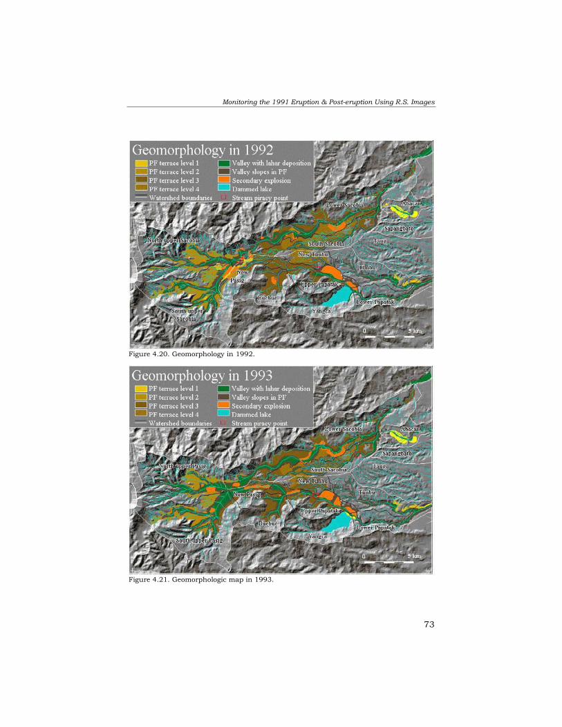
Monitoring the 1991 Eruption & Post-eruption Using R.S. Images
73
Figure 4.20. Geomorphology in 1992.
Figure 4.21. Geomorphologic map in 1993.
Chapter 4
74
4.5 Conclusions The high magnitude eruption of Mount Pinatubo has proven that available remote sensing is an indispensable tool in the assessment and monitoring of the impacts of volcanic eruptions. During the height of the eruption on 15-16 June 1991, the tephra fall was so thick and widespread that visual observation near the volcano was completely obscured. This is one of the major reasons that the volcano observatory was abandoned during the peak of the eruption. Monitoring the development of the climactic eruption was entirely monitored using remote sensing technology. Immediately after the eruption, the areas with pyroclastic flow deposits were very difficult to access and dangerous due to the occurrence of secondary explosions. Aerial photographs and satellite images were used to monitor geomorphic landforms and processes. Remnants of secondary explosion craters were clearly recognizable, making it possible to map their configuration and the resulting secondary pyroclastic flow deposits. The growth of several lahar-dammed lakes in highly inaccessible areas was monitored using remote sensing. These images were used to estimate the volume of impounding water and likewise predict the magnitude of possible lake breakout events. The development of gullies and channels were also monitored as well as the channel migration and stream piracies that have strong influence on the downstream lahar hazards. Lahars at Mt. Pinatubo affected areas with a size of several tens of square kilometres during one major event or hundreds of square kilometres per rainy season during the early years. The effects of siltation and flooding are more widespread. Owing to the scale and magnitude of these events, assessment could be done faster using remote sensing data if available than by using conventional field mapping. The repeat interval of most satellites are in the order of 16 to 26 days, i.e., for Landsat and Spot respectively. When the data are acquired on time, it will still be a faster method in synoptic-scale assessment. Vertical or oblique aerial photography still provides a very useful tool in rapid assessment of the geomorphic situation in a more detailed way. Monitoring the land cover changes and the vegetation recovery of the Mt. Pinatubo area has been done using multi-temporal satellite images. Change detection using remote sensing data has been widely used. However, when mapping the different volcanic deposits, some types of deposits show similar spectral characteristics. Several researchers at Mt. Pinatubo, such as Atienza (1995), Calomarde (1997) and Castro (1999), have also confirmed this problem. Differentiation of pyroclastic flows and dry lahars on the basis of their DN values proved to be
Monitoring the 1991 Eruption & Post-eruption Using R.S. Images
75
unreliable in some areas. Ground investigation has to be carried out in order to improve the image classification. After the complete burial of three drainage divides in the area, the initial slopes of the pyroclastic flow deposits played a major role in the early stream developments. Furthermore, most occurrences of the secondary explosions were developed along the axis of the buried pre-1991 major channels. This suggest that areas prone to major secondary explosions occur on places where pyroclastic flows are deposited with a thickness greater than 50 m. Likewise, these buried channels host subsurface water flows that may result in water saturation of the thick still-hot pyroclastic flow deposit leading to large secondary explosions. The newly developed major lahar channels followed the pre-1991 buried channels, and this suggests that underground channel flows have played a major role it the development of the new streams. The presence of relatively soft materials on the drainage divides, e.g. old pyroclastic flow deposits, made them susceptible to large-scale erosion. These divides were eroded during the occurrences of mass movements that were induced by large secondary explosions. Headward rain-induced erosion did not play a major role in the stream piracy. The unpredictable behaviour of stream capture events has contributed to the excessive cost of the mitigation structures in the downstream areas. During the first year, mitigation efforts were concentrated on the Abacan river, as this catchment has captured the major part of the upstream Sacobia watershed that lead to several large magnitude devastating syn-eruption lahars in the Abacan watershed. Therefore major engineering intervention structures were constructed in the Abacan river during the first year after the eruption. On April 4 1992, in the beginning of the second rainy season, the Sacobia river re-captured entirely the upper catchment of Abacan, making the newly built mitigation structures in the Abacan river obsolete while those in the Sacobia river were not capable for mitigating the large lahar events. Several villages and engineering structures were destroyed along the Sacobia river. Due to the drastic change in lahar delivery, engineering mitigation structures were then concentrated in the Sacobia River. By 04 October 1993, the Pasig river captured approximately 20 km² of the upper Sacobia catchment. This event resulted in several large lahar events in the Pasig river that destroyed several settlements downstream which were insufficiently protected by mitigation structures. On the other hand, the mitigation structures in the Sacobia river remained oversized in relation to the present lahar threat. Studying the geomorphic developments of Mt. Pinatubo’s watersheds played an important role in quantifying and determining the lahar hazards that can be expected in the major channels. The most

Chapter 4
76
important events to be monitored are the occurrence of stream piracies and the morphometric conditions of active channels. Such changes in the catchments should reflect the adjustments in the type of mitigation measures being performed in the particular channel.

Monitoring the 1991 Eruption & Post-eruption Using R.S. Images
77
Chapter 5: Quantitative Assessment of the Sediment Balance Using Multi-temporal Digital Terrain Models 5.1 Introduction The immediate concern of the authorities in the area surrounding Mt. Pinatubo after the eruption in 1991 was to assess the possible post-eruption hazards (secondary volcanic hazards) in the form of lahars. Owing to the large volume of pyroclastic flow deposits produced by the eruption, large magnitude lahars could be expected and they may continue to be a hazard for a substantial number of years. Therefore the scientists and people involved in disaster planning were faced with prediction and mitigation in respect to the long-term lahar hazard. Obviously, a prediction or forecast should be based on an understanding of how the new pyroclastic flow deposits will erode and deliver lahars through time. The initial important step was to know the volume of emplaced deposits per catchment and also the relationship of the rainfall intensity and magnitude and the frequency and magnitude of lahars. At Mt. Pinatubo, several authors have used different methods to quantify the volume of the emplaced pyroclastic flow deposits. These methods ranged from basically outlining the boundaries of pyroclastic flows on topographic maps, using oblique aerial photos, to detailed photogrammetric methods and some attempts to use radar interferometry (Castro, 1999) and airborne radar technology. This chapter deals mainly with the assessment of pyroclastic flow volumes and yearly erosion rates, using temporally acquired digital terrain models (DTM) that represent a particular period. Analog topographic maps, spot heights and existing DTMs were gathered from various sources from 1991 to 1996. Some estimates can be checked with results of the same temporal coverage that were derived by photogrammetric means. Some results were also compared with the number of lahars that were produced in the previous period. 5.2 Materials and methods The geomorphology of the Pinatubo catchments changes dramatically after every rainy season. The changes are so extensive that they can be monitored using aerial photographs and satellite images (see Chapter 4). To quantitatively monitor the volume of erosion and the remaining pyroclastic flow deposits, digital elevation models (DEMs) or DTMs are

Chapter 5
78
necessary. For this study one DTM per year was generated, representing the altitude of the terrain after the rainy season. Several researchers and some consulting firms made their own volumetric calculations, and some made their own DTMs for specific years. Among them are the Philippine Institute of Volcanology and Seismology (PHIVOLCS), the Japanese International Cooperating Agency (JICA), the United States Defense Mapping Agency (USDMA), the United States Army Corps of Engineers (USACE), the United States Geological Survey (USGS), the International Institute for Geo-information Science and Earth Observation (ITC), the Cartography and Remote Sensing Department of the University of the Philippines (UPCRS), and TOPSAR Airborne RADAR mission. The various parties involved in the volumetric calculations worked independently. Each group had their own resources and methods. For some years, several DTMs from different sources have been available, and this gave an opportunity to compare results and accuracies. DTMs are difficult to generate using conventional methods because they need a lot of resources and man-hours to create. Methods used to generate DTMs varied from group to group, and eventually each group worked with their own data formats. Analog contour maps and DTMs from different sources were converted to a common format. For this task of conversion, several software packages were used, including ArcInfo, ARCVIEW, ERDAS, ENVI, PCRASTER and ILWIS. Although there were some consultancy firms that created their own DTMs for the study area, their products were mostly restricted and digital copies of the DTMs were difficult to acquire. Most of the data were requested through various government protocols and eventually acquired at a later stage. Not all of the existing DTMs in the study area could be acquired for this study. Major changes in the catchment occur during the rainy season or lahar season, which is from June to November. Available DTMs should represent this situation either before or after the rainy season of the year. For naming conventions, we refer to the event of the lahar season in keywords, i.e., “post-1992 lahar”, meaning that the DTM represents the topographic conditions of the catchment after the 1992 rainy season, even if the data were acquired before the rainy season of the next year. In total there were 12 DTMs available for this study. Four of them were made using estimates from various oblique and vertical photographs (Daag, 1994; Daag and van Westen, 1996; and this work). From PHIVOLCS, JICA and UPCRS, contour maps in analog or digital format were obtained. The analog maps were then digitised and converted to DTMs, which required a lot of time. Altitude data from USDMA and a TOPSAR mission were digitally available, although in different data formats. One DTM that was generated by TOPSAR

Monitoring the 1991 Eruption & Post-eruption Using R.S. Images
79
airborne radar interferometry was difficult to use, since some areas did not have any information because of radar shadows, and some of the digital values were extremely high or low. The details of the different DTMs and the method by which they were derived are discussed in the next section. Table 5.1 lists all DTMs that were acquired and used in the analysis. 5.2.1 Pre-eruption DTMs These DTMs represent the topography prior to the 1991 eruption. • 1980 JICA DTM (dtm80j)
This DTM was created by the Japanese International Cooperating Agency (JICA) using analytic photogrammetric techniques. Contour lines were extracted from pre-eruption (1980) vertical photographs. Contour intervals were 5 m in the highlands and 2 m in the lowlands. These digital data were acquired only during the late stage of this research due to some copyright problems.
• 1986 DTM (dtm86a)
This DTM was produced by digitising the 1986 contour map of the United States Defence Mapping Agency (USDMA) at 1:50,000 scale. The map has contour intervals of 20 m in the highlands and 10 m in the lowlands. The map was digitised using ArcInfo software and later converted to ILWIS format. These maps were digitised under contract with an external digitising company. Contour lines were interpolated to produce a DTM with a resolution of 20 m.
• Pre-Eruption USDMA DTM (dtmuspre)
This DTM, produced by USDMA, was in ArcInfo grid format and covered a wider area, including other catchments. The data were captured before the 15 June 1991 eruption. The resolution of the original data was 100 m, which is lower than the resolution of 20 m used for all other DTMs. The data were resampled to 20 m to be able to integrate them in our analysis. However, the drawback was that it was more generalized than the other DTMs.
5.2.2 DTM shortly after the eruption • July 1991 DTM (dtmerpa)
After the main eruption, several calculations were made on the volume of the total 1991 pyroclastic flow deposits. However, none of them used the DTM overlaying technique because there were no vertical aerial photographs available for the period shortly after the eruption. In line with this, a DTM was created using a series of large-scale oblique photographs taken from low-flying helicopters.

Chapter 5
80
Heights and intersections of valley fills were marked and transferred to the pre-eruption contour map. A new contour map with the new pyroclastic flow deposits as valley fill was constructed. This was then digitised, rasterised and interpolated with a 20 m pixel resolution to produce the DTM. This DTM represents the pre-erosion condition of the pyroclastic flows and was used for the volume calculations of pyroclastic flows and the evaluation of erosion for the succeeding years.
5.2.3 Post-eruption DTMs 5.2.3.1 Post-1991 lahar • November 1991 JICA DTM (dtm91j)
This map was originally acquired as a topographic map sheet and digitised. Later it was also acquired in digital format. The source data were vertical panchromatic aerial photographs from 1991 with a scale of 1:15,000. These JICA maps are very detailed and they were used for the catchment boundary delineation and in the catchment-scale modelling described in Chapter 9.
• November 1991 DTM (dtm91a)
The DTM was derived using 1:15,000 scale vertical photographs, the same aerial photographs used in the 1991 JICA DTM. In order to make a more rapid erosion estimate a simple and more generalized method was used to generate the DTM. The method was based on estimates of the depth of the newly eroded channels obtained with the aid of a mirror stereoscope and a parallax bar. With the new channel morphometry, a new contour map was created in areas where there had been significant changes and masked over the pre-eruption DTM (dtm86a).
5.2.3.2 Post-1992 lahar • October 1992 JICA DTM (dtm92j)
The DTM was generated by photogrammetry extracted from the 1:25,000 scale vertical photographs taken in October 1992. Digital contour maps were acquired.
• October 1992 DTM (dtm92a)
The same set of vertical photographs was used as that taken by JICA to produce the 1992 DTM (dtm92j), but now using the parallax bar method.

Monitoring the 1991 Eruption & Post-eruption Using R.S. Images
81
• Post-eruption 1992 USDMA DTM (dtm92us) These data were acquired as a georeferenced DTM in ArcInfo raster format, with a pixel resolution of 100 m. The data were resampled to 20 m.
Table 5.1 List of all the DTMs used in this study.
DTM Name Date of
Acquisition; Represented
Date
Type of Acquisition
Method in Deriving DTM
Acquired Format
Geore-ferenced Source
dtm80j 1980
Topography; pre-eruption
Aerial Photography Photogrammetry Digital Yes JICA
dtm86a 1986
Topography; pre-eruption
Topographic Map
Digitising Contour Map Digital Yes USDMA
dtmpreus Pre-eruption Unknown Unknown Digital Yes
USDMA (Jones and Newhall,
1996)
dtmerpa
July-August 1991;
immediately after eruption with uneroded
PF deposit
Vertical and oblique aerial photograph
Photo Interpretation,
Digitising Analog No This work
dtm91a Nov 1991; post-1992
lahar season
Aerial Photography
Photo Interpretation,
Digitising Analog No This work
dtm92j October 1992;
post-1992 lahar season
Aerial Photography Photogrammetry Digital Yes JICA
dtm92us Nov 1992; post-1992
lahar season Unknown Unknown Digital Yes
USDMA (Jones and Newhall,
1996)
dtm93a April 1994; post-1993
lahar season
Aerial Photography
Photo Interpretation,
Digitising Analog No This work
dtm93j April 1994; post-1993
lahar season
Aerial Photography Photogrammetry Digital Yes JICA
dtm95up February 1996;
post-1995 lahar season
Aerial Photography Photogrammetry Analog No UP-CRSD
dtm96ts Nov 1996; post-1996
lahar season
Airborne Radar
Interferometry Interferometry Digital No TOPSAR
5.2.3.3 Post-1993 lahar • April 1994 DTM (dtm93a)
The data were derived using several oblique aerial photos to delineate the new changes in the pyroclastic flow deposits in April 1994. A contour map was generated by estimating the valley depths (eroded portions) after the 1993 lahar events. Valley depths were estimated by using the parallax bar method, supplemented by numerous field height measurements.
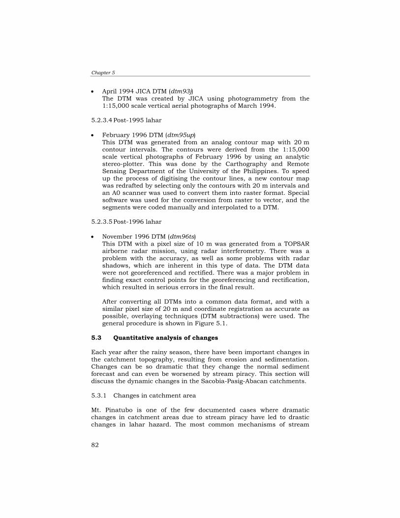
Chapter 5
82
• April 1994 JICA DTM (dtm93j) The DTM was created by JICA using photogrammetry from the 1:15,000 scale vertical aerial photographs of March 1994.
5.2.3.4 Post-1995 lahar • February 1996 DTM (dtm95up)
This DTM was generated from an analog contour map with 20 m contour intervals. The contours were derived from the 1:15,000 scale vertical photographs of February 1996 by using an analytic stereo-plotter. This was done by the Carthography and Remote Sensing Department of the University of the Philippines. To speed up the process of digitising the contour lines, a new contour map was redrafted by selecting only the contours with 20 m intervals and an A0 scanner was used to convert them into raster format. Special software was used for the conversion from raster to vector, and the segments were coded manually and interpolated to a DTM.
5.2.3.5 Post-1996 lahar • November 1996 DTM (dtm96ts)
This DTM with a pixel size of 10 m was generated from a TOPSAR airborne radar mission, using radar interferometry. There was a problem with the accuracy, as well as some problems with radar shadows, which are inherent in this type of data. The DTM data were not georeferenced and rectified. There was a major problem in finding exact control points for the georeferencing and rectification, which resulted in serious errors in the final result. After converting all DTMs into a common data format, and with a similar pixel size of 20 m and coordinate registration as accurate as possible, overlaying techniques (DTM subtractions) were used. The general procedure is shown in Figure 5.1.
5.3 Quantitative analysis of changes Each year after the rainy season, there have been important changes in the catchment topography, resulting from erosion and sedimentation. Changes can be so dramatic that they change the normal sediment forecast and can even be worsened by stream piracy. This section will discuss the dynamic changes in the Sacobia-Pasig-Abacan catchments. 5.3.1 Changes in catchment area Mt. Pinatubo is one of the few documented cases where dramatic changes in catchment areas due to stream piracy have led to drastic changes in lahar hazard. The most common mechanisms of stream

Monitoring the 1991 Eruption & Post-eruption Using R.S. Images
83
piracy are headward erosion or the overtopping of the drainage divides by extreme accumulation of materials. At Mt. Pinatubo, the mechanism is rather unique, in the sense that changes are produced by the effects of secondary explosions and secondary pyroclastic flow generation due to the remobilisation of hot pyroclastic flow deposits. The process of stream capture occurs as a single event, lasting a few hours. Although these types of events are difficult to predict, they should be taken into account in assessing future hazards. Four important stream piracy events have occurred in the study area (see Chapter 4). The first was immediately after the eruption, when most pyroclastic flow deposits overtopped the three drainage divides of Pasig, Sacobia and Abacan. This was the first geomorphic impact during the crisis because there were no clear drainage boundaries that could be established. It took several weeks during the rainy season to re-establish a new channel network. Due to numerous large-scale lahar events in the Abacan River in the first year, it appeared that Abacan had captured at least 5 km2 of the upper Sacobia catchment, extending its pre-eruption catchment boundaries. The increase of 5 km2 was only interpreted at the end of the rainy season because that was when the first vertical photographs were taken. Considering the number of lahars that flowed into the Abacan channel during that rainy season, there must have been an undocumented larger stream piracy to justify the volume of flows in the Abacan channel. Concurrently, the lahars at Sacobia River were negligible, although it had a large pre-eruption catchment size. This prompted the civil authorities to take extensive protective measures in the Abacan channel because it passes through a highly populated area in Angeles City. The first documented case of stream piracy occurred on 4 April 1992 during a dry period, just before the beginning of the second lahar season. The event led to the re-capture of Abacan by Sacobia and significantly reduced the headwater and pyroclastic flow source materials of Abacan by 5.5 km2 of catchment. This occurred about a kilometre upstream of the bifurcation point between the two channels. The capture was initiated by a secondary pyroclastic flow that eroded deeply into the Sacobia channel, thereby cutting off the Abacan headwaters. This event practically averted the lahar danger in the Abacan Valley. After the capture, the Sacobia River began experiencing several large destructive lahars. Remedial measures were therefore focused on the Sacobia channel. The next stream capture event was the most significant that had ever occurred in the catchment system. It happened on 4 October 1993, in the middle of the rainy season. The event was caused by extensive secondary pyroclastic flows that occurred at the confluence of the north and south upper Sacobia channel (see Figure 5.6). This site had a very

Chapter 5
84
thick cover of pyroclastic flow deposits. The events caused degradations in the upper catchment boundary of Pasig and led to the capture of approximately 20 km2 of the upper Sacobia catchment (see Figure 4.21). These events had significant impacts on the downstream parts of the Pasig channel, where succeeding lahar events were several orders of magnitudes larger than the pre-capture events. Unfortunately, expensive mitigation measures had already been taken in the Sacobia channel but not in the downstream part of the Pasig catchment. Since that event, Pasig has remained the most destructive channel and the capture has remained permanent. Table 5.2 and Figure 5.2 show the comparative catchment areas in four different periods. Figures 5.3, 5.4, 5.5 and 5.6 illustrate graphically the changes in the catchment systems and the pyroclastic flow distribution in four periods.
YEAR SACOBIA PASIG ABACAN TOTAL
PRE - ERUPTION POST–ERUPTION 1992 1994
38 33 38 18
24 24 24 44
2 7 2 2
64 64 64 64
Table 5.2. Changes in catchment size in the three catchment systems on the east side of Mt. Pinatubo. Values are rounded off and are in square kilometres. The change in total area is due to the formation of the crater.
Figure 5.1 Flow diagram showing the series of DTMs and how they arederived. It shows also the procedures in the volumetric calculation.
PRE-ERUPTION DTMs POST-PLINIAN 1991 1992 DTMs1993 1995 199619921980
AERIAL PHOTOS
GENERATIONOF 5m
CONTOURUSING
ANALYTICALINSTRUMENTS
RASTERIZEDTO 20m
PIXEL ANDINTERPOLATED
1980 PRE-ERUPTION
DTM(dtm80j)
1986 PRE-ERUPTION
DTM(dtm86a)
1986 USDMACONTOUR MAP
1:50,000
DIGITIZED20m CONTOUR
INTERVAL
RASTERIZEDTO 20m
PIXEL ANDINTERPOLATED
EXTENDEDCONTOURS
ACROSSDEPOSIT
LARGE-SCALESEMI-VERTICAL
AERIALPHOTOS JULY
1991
DIGITIZEDPF VALLEY FILL
OUTLINE
RASTERIZED IN20m PIXEL ANDINTERPOLATED
POST PLINIANDTM
(dtmerpc)
VERTICALPHOTOSNOV 1991
VERTICALPHOTOSNOV 1992
OBLIQUEPHOTOSAPR 1994
INTERPRET AND PLOT VALLEYS & MAJOR GULLIES
MEASURE VALLEY DEPTHS AND MAJOR GULLIES
RECREATE VALLEYS AND MAJOR GULLIES
PARRALAX BAR AND FIELD ESTIMATES
MASK NEW VALLEYS AND MAJOR GULLIES IN THEPREVIOUS DTM AND GENERATE NEW DTM
POST- LAHAR1991 DTM(dtm91a)
POST- LAHAR1992 DTM(dtm92a)
POST LAHAR1993 DTM(dtm93a)
VERTICALPHOTOSOCT 19921:25,000
GENERATIONOF 5m
CONTOURUSING
ANALYTICALINSTRUMENTS
RASTERIZEDTO
20m PIXEL ANDINTERPOLATED
POST - LAHAR1992 DTM(dtm92j)
VERTICALPHOTOS
MARCH 19941:15,000 SCALE
GENERATIONOF 5m
CONTOURUSING
ANALYTICALINSTRUMENTS
RASTERIZEDTO 20m PIXEL
ANDINTERPOLATED
POST - LAHAR1993 DTM(dtm93j)
USDMA100m PIXEL
PRE-ERUPTIONDIGITAL DTM
RESAMPLEDTO 20m PIXELRESOLUTION
PRE-ERUPTIONDTM
(dtmuspre)
RECTIFIED ANDGEOREFE-RENCED
RESAMPLE TO20m PIXEL
RESOLUTION
USDMA100m PIXEL
RESOLUTIONNOV 1992
POST - LAHAR1992 DTM(dtm92us)
RECTIFIED ANDGEOREFER-
RENCED
POST - LAHAR1996 DTM(dtm96ts)
TOPSARDTM 10m PIXELRESOLUTION
NOV 96
ROTATED ANDRESAMPLED
GEOREFE-RENCED
VERTICALPHOTOSFEB 19961:15,000SCALE
GENERATIONOF CONTOUR
BYPHOTOGRAM-
METRY
DIGITIZECONTOURS
RASTERIZEDTO 20m PIXEL
ANDINTERPOLATED
POST - LAHAR1995 DTM(dtm95up)
1993
OVERLAY
1991 TOTALPF
VOLUME
OVERLAY
1991 TOTAL PFVOLUME(USDMA)
OVERLAY
1991 TOTAL PFVOLUME
OVERLAY
POST-LAHAR1991 TOTAL
EROSIONVOLUME
OVERLAY
POST-LAHAR1992 TOTAL
EROSIONVOLUME
OVERLAY
OVERLAY
OVERLAY
OVERLAY
OVERLAY
OVERLAY
POST-LAHAR1993 TOTAL
EROSIONVOLUME
POST-LAHAR1996 TOTAL
EROSIONVOLUME
POST-LAHAR1995 TOTAL
EROSIONVOLUME
POST-LAHAR1993 TOTAL
EROSIONVOLUME
POST-LAHAR1992 TOTAL
EROSIONVOLUME
POST-LAHAR1992 TOTAL
EROSIONVOLUME
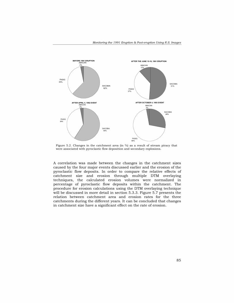
Monitoring the 1991 Eruption & Post-eruption Using R.S. Images
85
A correlation was made between the changes in the catchment sizes caused by the four major events discussed earlier and the erosion of the pyroclastic flow deposits. In order to compare the relative effects of catchment size and erosion through multiple DTM overlaying techniques, the calculated erosion volumes were normalized in percentage of pyroclastic flow deposits within the catchment. The procedure for erosion calculations using the DTM overlaying technique will be discussed in more detail in section 5.3.3. Figure 5.7 presents the relation between catchment area and erosion rates for the three catchments during the different years. It can be concluded that changes in catchment size have a significant effect on the rate of erosion.
BEFORE 1991 ERUPTION
PASIG35%
SACOBIA62%
ABACAN3%
AFTER THE JUNE 15-16, 1991 ERUPTION
PASIG37%
ABACAN12%
SACOBIA51%
AFTER APRIL 4, 1992 EVENT
PASIG38%
SACOBIA59%
ABACAN3%
AFTER OCTOBER 4, 1993 EVENT
PASIG69%
ABACAN3%
SACOBIA28%
.
Figure 5.2. Changes in the catchment area (in %) as a result of stream piracy thatwere associated with pyroclastic flow deposition and secondary explosions.

Chapter 5
86
Figure 5.3. Map showing the thickness distribution of the June 1991pyroclastic flow deposits in relation to the pre-eruption catchmentboundaries.
Figure 5.4. The new pyroclastic flow deposits overtopped the drainagedivides and changed the catchment dimensions. The largest changetook place in the Abacan catchment, which captured an additional 5.47km2 (350% of its original size) of the Sacobia catchment, resulting inunexpectedly large magnitude lahars during the first year.
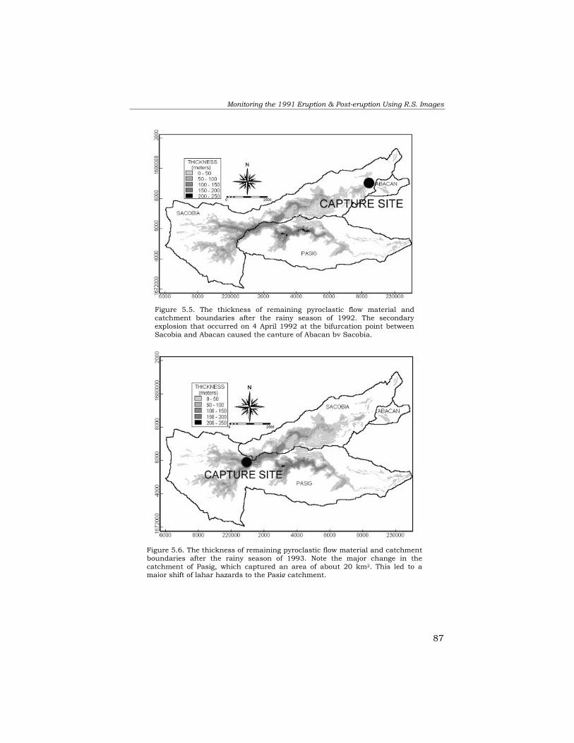
Monitoring the 1991 Eruption & Post-eruption Using R.S. Images
87
Figure 5.5. The thickness of remaining pyroclastic flow material andcatchment boundaries after the rainy season of 1992. The secondaryexplosion that occurred on 4 April 1992 at the bifurcation point betweenSacobia and Abacan caused the capture of Abacan by Sacobia.
Figure 5.6. The thickness of remaining pyroclastic flow material and catchmentboundaries after the rainy season of 1993. Note the major change in thecatchment of Pasig, which captured an area of about 20 km2. This led to amajor shift of lahar hazards to the Pasig catchment.
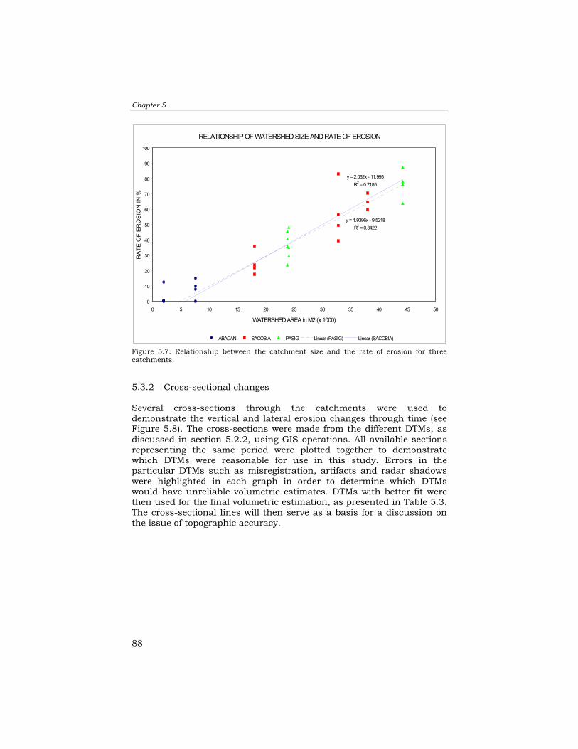
Chapter 5
88
5.3.2 Cross-sectional changes Several cross-sections through the catchments were used to demonstrate the vertical and lateral erosion changes through time (see Figure 5.8). The cross-sections were made from the different DTMs, as discussed in section 5.2.2, using GIS operations. All available sections representing the same period were plotted together to demonstrate which DTMs were reasonable for use in this study. Errors in the particular DTMs such as misregistration, artifacts and radar shadows were highlighted in each graph in order to determine which DTMs would have unreliable volumetric estimates. DTMs with better fit were then used for the final volumetric estimation, as presented in Table 5.3. The cross-sectional lines will then serve as a basis for a discussion on the issue of topographic accuracy.
Figure 5.7. Relationship between the catchment size and the rate of erosion for threecatchments.
RELATIONSHIP OF WATERSHED SIZE AND RATE OF EROSION
y = 1.9396x - 9.5218R2 = 0.8422
y = 2.062x - 11.995R2 = 0.7185
0
10
20
30
40
50
60
70
80
90
100
0 5 10 15 20 25 30 35 40 45 50
WATERSHED AREA in M2 (x 1000)
RAT
E O
F ER
OSI
ON
IN %
ABACAN SACOBIA PASIG Linear (PASIG) Linear (SACOBIA)

Monitoring the 1991 Eruption & Post-eruption Using R.S. Images
89
In total, seven cross-sections were made across the catchment, labelled from A-A’ to G-G’ (see Figures 5.9 to 5.15). For each cross-section altitudes were obtained from the 12 different DTMs mentioned in section 5.2.2 (see Table 5.1). The 12 cross-sections are presented in groups to improve clarity in the presentation and discussion. In each group, the post-eruption DTM (dtmerpa, in heavy solid line) served as a baseline for correlating other sections of different times. The groupings are as follows: • The first series of graphs (Figures 5.9A to 5.15A) consists of three
cross-sections that represent all pre-eruption DTMs taken from various sources (dtm86a, dtm80j, and dtmpreus).
• The next series of figures (5.9B to 5.15B) represents the two-year
period after eruption (1991 and 1992, i.e., dtm91a, dtm92us, dtm92a and dtm92j).
• The last series of figures (5.9C to 5.15C) represents the years 1993,
1995 and 1996 (dtm93a, dtm93j, dtm95up, dtm96ts).
Figure 5.8. Map showing the locations of seven cross-sections.

Chapter 5
90
5.3.2.1 Results The following discussion will focus on the temporal changes in each cross-section and will also show how the erosion evolved in the five years after the eruption. The location of the first cross-section (line A-A’, see Figure 5.9) with a length of 3.9 km is within 1.2 km of the crater. There was no significant change in altitude before or after the eruption (except for the stripped forest mantle) and the dominant process here during the eruption was mostly the stripping of vegetation and extensive transportation of pyroclastic flow deposits to lower altitudes. This area consists of highly indurated ancient Pinatubo deposits. In conjunction, the transport energy of the pyroclastic flow was so high that no deposition took place in this area.
Line B-B’ (Figure 5.10) is about 2.9 km east of the crater, and the cross-sectional line is about 5.1 km long. The maximum thickness of the pyroclastic flow deposits was 150 m and there seems to be a hill-shaped artifact caused by the dtm96ts, which is not represented in Figure 5.10A. Figure 5.10B shows an exaggerated level of erosion from dtm92us, which is not present in other sections of the same date. It also shows that active erosion is high on the left side of the bank (southern part), which served as the main channel for the upstream catchment. Figure 5.10C shows more aggressive erosion in the left bank, and this represents the situation after the significant stream capture. It can be noted that erosion proceeded even deeper than the pre-eruption topography, as represented by the 1995 cross-section (dtm95up). Line C-C’ (Figure 5.11) is located 5.3 km east of the crater and the section is about 2.5 km long. It represents the narrowest section of the catchment but has a thick pyroclastic flow accumulation. Thickness reached nearly 200 m, as presented in Figure 5.11A. It can be observed that in Figure 5.11B specifically the post-eruption DTM (dtm92us) shows no good matching, even on areas where there should be no changes, i.e., on the right side of the bank. From Figure 5.11C, it can be concluded that the DTM generated from TOPSAR data (dtmt95c) has large inherent errors, as illustrated by some artificial hills on the right side. In fact neither large-scale erosion nor deposition affected these areas. The deep erosion zones represented in Figure 5.11C (dtm95up), where erosion had reached the pre-eruption deposits, were confirmed during the fieldwork. The erosion lines shown by dtm92a are generalized because the valleys were only measured using a parallax bar and some field checks. Line D-D’ (Figure 5.12) is located 6.2 km east of the crater and the cross-section is 3.8 km long. This area has the thickest pyroclastic flow

Monitoring the 1991 Eruption & Post-eruption Using R.S. Images
91
deposit, reaching about 250 m, and buried the 120 m high marking the hill drainage divide separating Pasig and Sacobia (see Figure 5.12A). It appears from Figure 5.12B that there was minimal erosion at this section until 1992, even though there may have been several lahars passing the area. This site must have been a zone where erosion and lahar accumulation were more or less in balance. Figure 5.12C shows the section from 1993 to 1996. It appears that there was extensive erosion during this period. It can also be noted, based on the 1995 DTMs (dtm95up), that the erosion had proceeded deeper than the pre-eruption level. Noteworthy is the erosion of the hill (drainage divide) that occurred after the capture. Line E-E’ (Figure 5.13) is 8.1 km from the crater and the section is 5.4 km long. Along this line, the maximum thickness of the deposits was about 125 m in the Sacobia channel (Figure 5.13A). Erosion was relatively limited until 1992, in the order of 50 m deep, forming narrow gullies (Figure 5.13B). By 1996 (Figure 5.13C) erosion had removed almost all pyroclastic flow materials and had nearly reached the pre-eruption level. Line F-F’ (Figure 5.14) is about 9.8 km from the crater and the section is 6.4 km long. The thickness of the pyroclastic flow deposits was high in the deep pre-eruption valleys and reached a maximum of about 100 m. Also here it appears that erosion was not very strong in the area. In fact this site was subjected to many erosion and aggradation alternations, depending on the nature of lahar events, which were more or less in balance. Line G-G’ (Figure 5.15) is 10.3 km away from the crater and the cross-section is 6 km long. There are no data in the middle of the graph because this part belongs to another lower catchment, which was not affected by the pyroclastic flow deposition and was not included in the DTM. Thickness of the deposit along the deep valleys is in the order of 50 m. It appears in this part that erosion has proceeded down to the base or even deeper than the pre-eruption channel floor.
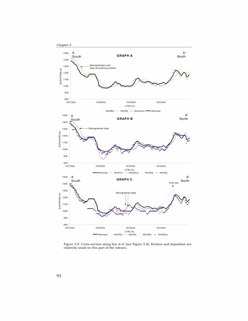
Chapter 5
92
Figure 5.9. Cross-section along line A–A’ (see Figure 5.8). Erosion and deposition arerelatively small on this part of the volcano.
GRAPH A
800
900
1000
1100
1200
1300
1400
1500
1677540 1676540 1675540 1674540UTM (m)
ELEV
ATIO
N (m
)
dtm86a dtm80j dtmpreus dtmerpa
Misregistration anddata smoothing problem
ASouth
A'North
GRAPH B
800
900
1000
1100
1200
1300
1400
1500
1677540 1676540 1675540 1674540UTM (m)
ELEV
ATIO
N (m
)
dtmerpa dtm91a dtm92us dtm92a dtm92j
Misregistered data
ASouth
A'North
GRAPH C
800
900
1000
1100
1200
1300
1400
1500
1677540 1676540 1675540 1674540UTM (m)
ELEV
ATIO
N (m
)
dtmerpa dtm93a dtm93j dtm96ts dtm95up
Misfit data
ASouth
A'North
Misregistered data

Monitoring the 1991 Eruption & Post-eruption Using R.S. Images
93
Figure 5.10. Cross-section along line B–B’ (see Figure 5.8). Erosion is more rapid inthe left (south) channel. Erosion in 1995 has scoured even the pre-eruption channelfloor.
G RAPH A
750
800
850
900
950
1000
1050
1100
1677660 1676660 1675660 1674660 1673660 1672660UTM (m )
ELEV
ETIO
N (m
)
d tm 86a dtm 80j dtm preus dtm erpa
Misregistration and data sm oothing
SO UTH U PPER SAC O BIA
N O RTH U PPER SAC OBIA
BSouth
B 'North
G RAPH B
750
800
850
900
950
1000
1050
1100
1677660 1676660 1675660 1674660 1673660 1672660UTM (m )
ELEV
ATIO
N (m
)
d tm erpa dtm 91a dtm 92us dtm 92a dtm 92j
M isregistered and exaggerated data
BSouth
B 'North
G RAPH C
750
800
850
900
950
1000
1050
1100
1677660 1676660 1675660 1674660 1673660 1672660UTM (m )
ELEV
ATIO
N (m
)
d tm erpa dtm 93a dtm 93j dtm 96ts dtm 95up
Artifacts and m isregistered data
Erosion artifact
B 'North
BSouth
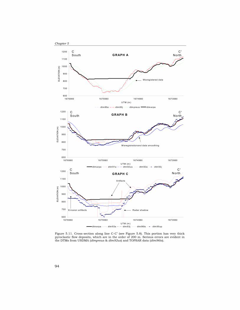
Chapter 5
94
Figure 5.11. Cross-section along line C–C’ (see Figure 5.8). This portion has very thickpyroclastic flow deposits, which are in the order of 200 m. Serious errors are evident inthe DTMs from USDMA (dtmpreus & dtm92us) and TOPSAR data (dtm96ts).
G RAPH B
600
700
800
900
1000
1100
1200
1676980 1675980 1674980 1673980U TM (m )
ELEV
ATIO
N (m
)
d tm erpa dtm 91a dtm 92us dtm 92a dtm 92j
Misregistrationand data sm oothing
CSouth
C 'North
G RAPH A
600
700
800
900
1000
1100
1200
1676980 1675980 1674980 1673980UTM (m )
ELEV
ATIO
N (m
)
d tm 86a dtm 80j dtm preus dtm erpa
Misregistered data
CSouth
C 'North
G RAPH C
600
700
800
900
1000
1100
1200
1676980 1675980 1674980 1673980U TM (m )
ELEV
ATIO
N (m
)
d tm erpa dtm 93a dtm 93j dtm 96ts dtm 95up
Radar shadow
Artifacts
Errosion artifacts
C 'North
CSouth
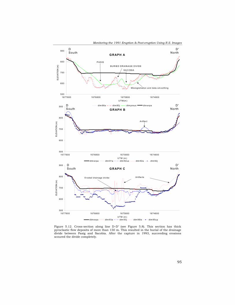
Monitoring the 1991 Eruption & Post-eruption Using R.S. Images
95
Figure 5.12. Cross-section along line D–D’ (see Figure 5.8). This section has thickpyroclastic flow deposits of more than 150 m. This resulted in the burial of the drainagedivide between Pasig and Sacobia. After the capture in 1993, succeeding erosionsscoured the divide completely.
G RAPH A
500
600
700
800
900
1677800 1676800 1675800 1674800UTM(m )
ELEV
ATIO
N (m
)
d tm 86a dtm 80j dtm preus dtm erpa
Misregistration and data sm oothing
BU RIED DR AIN AG E DIV IDE
PASIG
SAC O BIA
DSouth
D 'North
G RAPH B
500
600
700
800
900
1677800 1676800 1675800 1674800U TM (m )
ELEV
ATIO
N (m
)
d tm erpa dtm 91a dtm 92us dtm 92a dtm 92j
Artifact
DSouth
D 'North
G RAPH C
500
600
700
800
900
1677800 1676800 1675800 1674800U TM (m )
ELEV
ATIO
N (m
)
d tm erpa dtm 93a dtm 93j dtm 96ts dtm 95up
ArtifactsEroded drainage divide
DSouth
D 'North

Chapter 5
96
Figure 5.13. Cross-section along line E–E’ (see Figure 5.8). Pyroclastic flow deposits arethicker in the Sacobia channel, and also the erosion is deeper in this section, as shownin the 1995 cross-section.
G RAPH A
300
400
500
600
700
800
1678900 1677900 1676900 1675900 1674900 1673900
U TM (m )
ELEV
ATIO
N (m
)
d tm 86a dtm 80j dtm preus dtm erpa
Misregistered andexaggerated data
PASIG SAC O BIA
ESouth
E 'North
G RAPH B
300
400
500
600
700
800
1678900 1677900 1676900 1675900 1674900 1673900U TM (m )
ELEV
ATIO
N (m
)
d tm erpa dtm 91a dtm 92us dtm 92a dtm 92j
O ffset data
O ffset data
ESouth
E 'North
G RAPH C
300
400
500
600
700
800
1678900 1677900 1676900 1675900 1674900 1673900
UTM (m )
ELEV
ATIO
N (m
)
d tm erpa dtm 93a dtm 93j dtm 96ts dtm 95up
Radar shadows
Artifacts
ESouth
E 'North
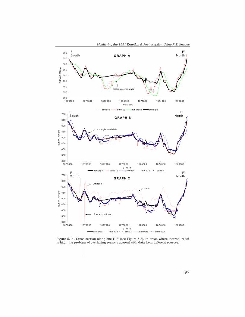
Monitoring the 1991 Eruption & Post-eruption Using R.S. Images
97
Figure 5.14. Cross-section along line F–F’ (see Figure 5.8). In areas where internal reliefis high, the problem of overlaying seems apparent with data from different sources.
G RAPH A
300
350
400
450
500
550
600
650
700
1679800 1678800 1677800 1676800 1675800 1674800 1673800U TM (m )
ELEV
ATIO
N (m
)
d tm 86a dtm 80j dtm preus dtm erpa
Misregistered data
FSouth
F'North
G RAPH B
300
350
400
450
500
550
600
650
700
1679800 1678800 1677800 1676800 1675800 1674800 1673800U TM (m )
ELEV
ATIO
N (m
)
d tm erpa dtm 91a dtm 92us dtm 92a dtm 92j
M isregistered data
FSouth
F'North
G RAPH C
300
350
400
450
500
550
600
650
700
1679800 1678800 1677800 1676800 1675800 1674800 1673800U TM (m )
ELEV
ATIO
N (m
)
d tm erpa dtm 93a dtm 93j dtm 96ts dtm 95up
Misfit
R adar shadows
Artifacts
FSouth
F'North

Chapter 5
98
Figure 5.15. Cross-section along line G–G’ (see Figure 5.8). Middle portion of the sectionshas no data because it intersects another catchment that is not part of the study area.
G RAPH A
250
300
350
400
450
500
550
1679900 1678900 1677900 1676900 1675900 1674900 167390U TM (m )
ELEV
ATIO
N (m
)
d tm 86a dtm 80j dtm preus dtm erpa
SEPAR ATEC ATC HMENT
Misregistered data
GSouth
G 'North
G RAPH B
250
300
350
400
450
500
550
1679900 1678900 1677900 1676900 1675900 1674900 167390U TM (m )
ELEV
ATIO
N (m
)
d tm erpa dtm 91a dtm 92us dtm 92a dtm 92j
SEPARATEC ATC HMEN T
GSouth
G 'North
G RAPH C
250
300
350
400
450
500
550
1679900 1678900 1677900 1676900 1675900 1674900 167390U TM (m )
ELEV
ATIO
N (m
)
d tm erpa dtm 93a dtm 93j dtm 96ts dtm 95up
R adar shadow
Artifact and m isfit data
SEPAR ATE C ATC HMENT
GSouth
G 'North

Monitoring the 1991 Eruption & Post-eruption Using R.S. Images
99
5.3.3 Volumetric changes and erosion Volumetric calculations were done by means of DTM overlaying techniques. (The procedure was discussed in section 5.2.2.) To aggregate the results per catchment (i.e., Abacan, Pasig and Sacobia), a catchment map was combined with the raster maps containing the erosion volume. Since the catchment divides have changed four times (different boundaries during pre-eruption, post-eruption, 1992 and 1994), the calculation of erosion volume in a certain year has to include the catchment area changes. Calculating the volume changes for several years can be done according to two methods. The first method is to subtract the DTMs progressively each year (Figure 5.16). This method is dependent on the input of the preceding year and the output will be used for the succeeding year. The method is good if all the temporal DTMs have a reasonable accuracy. However, since the DTMs were collected from various sources, there are some inherent relative errors that make this method less suitable. Also, the resulting error propagation cannot be managed. A better approach to calculating the volume independently is to calculate the volume changes in parallel. Each DTM is compared with one fixed DTM, for which the post-eruption DTM (dtmerpa) is used. The latter method was adopted in this research (Figure 5.17). Some sample maps that calculate the remaining volumes per year are shown in a series of graphs (Figures 5.18 to 5.21). Based on the series of cross-sections presented before, it was observed in some data sets that considerable errors also occur in areas that are known to be stable. These are on the mountainsides where there were no recent pyroclastic flow deposits. The stable or resistant areas are made of ancient Pinatubo deposits that are highly indurated and are resistant to erosion. To drastically eliminate the errors in the volume calculation, these areas were excluded from the calculations for erosion. A mask was prepared so that erosion was only calculated within the boundaries of the 1991 pyroclastic flows. The series of maps (Figures 5.18 to 5.21) shows a few samples of the spatial distribution of the remaining pyroclastic flow materials in different years. It can be seen on the maps that there are white spaces (masked areas) near the catchment boundaries and in the middle of the pyroclastic flow field, i.e., unburied hills were excluded on purpose because these are the areas where there has been no significant erosion.
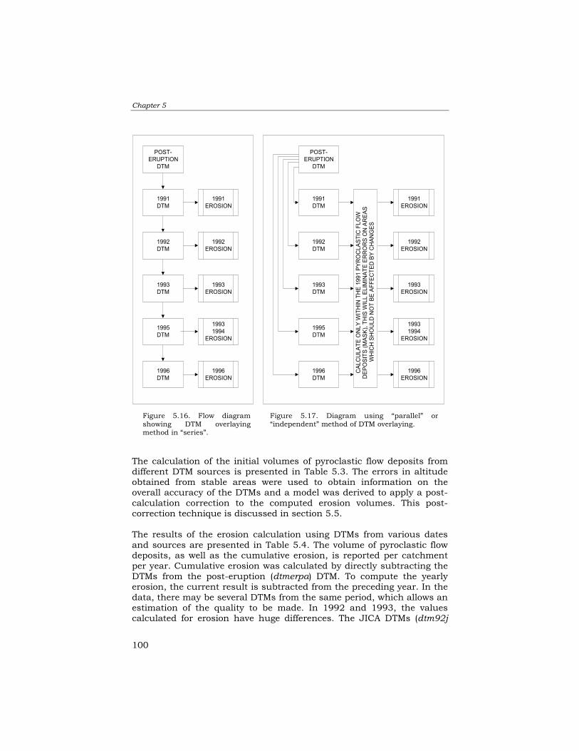
Chapter 5
100
The calculation of the initial volumes of pyroclastic flow deposits from different DTM sources is presented in Table 5.3. The errors in altitude obtained from stable areas were used to obtain information on the overall accuracy of the DTMs and a model was derived to apply a post-calculation correction to the computed erosion volumes. This post-correction technique is discussed in section 5.5. The results of the erosion calculation using DTMs from various dates and sources are presented in Table 5.4. The volume of pyroclastic flow deposits, as well as the cumulative erosion, is reported per catchment per year. Cumulative erosion was calculated by directly subtracting the DTMs from the post-eruption (dtmerpa) DTM. To compute the yearly erosion, the current result is subtracted from the preceding year. In the data, there may be several DTMs from the same period, which allows an estimation of the quality to be made. In 1992 and 1993, the values calculated for erosion have huge differences. The JICA DTMs (dtm92j
POST-ERUPTION
DTM
1991DTM
1992DTM
1993DTM
1995DTM
1992DTM
1996DTM
1991EROSION
1992EROSION
1993EROSION
19931994
EROSION
1996EROSION
POST-ERUPTION
DTM
1991DTM
1993DTM
1995DTM
1996DTM
1991EROSION
1992EROSION
1993EROSION
19931994
EROSION
1996EROSION
CAL
CU
LATE
ON
LY W
ITH
IN T
HE
1991
PYR
OC
LAST
IC F
LOW
DEP
OSI
TS (M
ASK)
, TH
IS W
ILL
ELIM
INAT
E ER
RO
RS
ON
AR
EAS
WH
ICH
SH
OU
LD N
OT
BE A
FFEC
TED
BY
CH
ANG
ES
Figure 5.16. Flow diagramshowing DTM overlayingmethod in “series”.
Figure 5.17. Diagram using “parallel” or“independent” method of DTM overlaying.
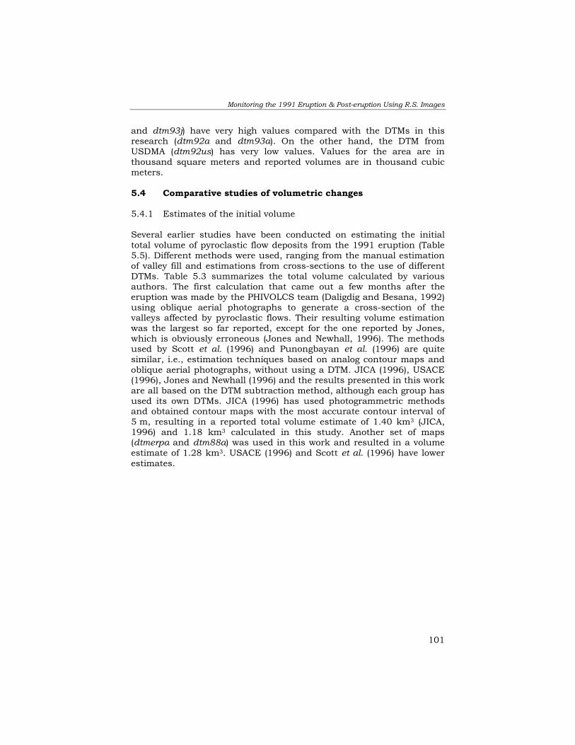
Monitoring the 1991 Eruption & Post-eruption Using R.S. Images
101
and dtm93j) have very high values compared with the DTMs in this research (dtm92a and dtm93a). On the other hand, the DTM from USDMA (dtm92us) has very low values. Values for the area are in thousand square meters and reported volumes are in thousand cubic meters. 5.4 Comparative studies of volumetric changes 5.4.1 Estimates of the initial volume Several earlier studies have been conducted on estimating the initial total volume of pyroclastic flow deposits from the 1991 eruption (Table 5.5). Different methods were used, ranging from the manual estimation of valley fill and estimations from cross-sections to the use of different DTMs. Table 5.3 summarizes the total volume calculated by various authors. The first calculation that came out a few months after the eruption was made by the PHIVOLCS team (Daligdig and Besana, 1992) using oblique aerial photographs to generate a cross-section of the valleys affected by pyroclastic flows. Their resulting volume estimation was the largest so far reported, except for the one reported by Jones, which is obviously erroneous (Jones and Newhall, 1996). The methods used by Scott et al. (1996) and Punongbayan et al. (1996) are quite similar, i.e., estimation techniques based on analog contour maps and oblique aerial photographs, without using a DTM. JICA (1996), USACE (1996), Jones and Newhall (1996) and the results presented in this work are all based on the DTM subtraction method, although each group has used its own DTMs. JICA (1996) has used photogrammetric methods and obtained contour maps with the most accurate contour interval of 5 m, resulting in a reported total volume estimate of 1.40 km3 (JICA, 1996) and 1.18 km3 calculated in this study. Another set of maps (dtmerpa and dtm88a) was used in this work and resulted in a volume estimate of 1.28 km3. USACE (1996) and Scott et al. (1996) have lower estimates.

Chapter 5
102
Figure 5.18. Distribution of the remaining pyroclastic flows after one rainyseason. DTM used: dtmerpa - dtm91a
Figure 5.19. Distribution of the remaining pyroclastic flow deposits in 1992.DTM used: dtmerpa – dtm92j.

Monitoring the 1991 Eruption & Post-eruption Using R.S. Images
103
Figure 5.21. Spatial distribution of pyroclastic flow materials at the end of the1995 lahar season. In many areas all pyroclastic flow material has been erodedand the underlying pre-eruption materials are exposed. DTMs used are: dtmerpa –dtm95up.
Figure 5.20. Distribution of remaining pyroclastic flow deposits after three rainyseasons. DTMS used are dtmerpa - dtm93a.

Chapter 5
104
Table 5.3. Calculated volumes of the initial pyroclastic flow deposit from three different DTM sources.
INITIAL VOLUME OF PYROCLASTIC FLOWS (In thousand cubic meters)
Year (DTM)
SACOBIA PASIG ABACAN TOTAL
PRE (dtm81j) 652 414 91 1,157
PRE (dtm86a) 631 517 128 1,276
PRE dtmuspre) 454 527 174 1,155
Table 5.4. Results of the yearly erosion calculations using different DTM sources.
TOTAL ERODED VOLUME PER CATCHMENT RESULTS FROM 3 CATCHMENTS YEAR
(DTM)
SACOBIA PASIG ABACAN CUM. EROSION
YEARLY EROSION
REMAINING VOLUME
1991 (dtm91a) 98.9 77.9 25.2 202.0 202.0 1,073.4
1992 (dtm92j) 290.3 121.0 0.1 411.4 209.4 863.9
1992 (dtm92a) 193.7 105.0 1.3 300.0 98.0 975.4
1992 (dtm92us) 168.6 47.9 13.4 229.9 27.9 1,045.5
1993 (dtm93j) 567.6 159.1 2.6 729.3 317.9 546.1
1993 (dtm93a) 143.2 253.4 1.4 398.0 98.0 877.4
1995 (dtm95up)
Unusual value 840.3 2.6 842.9 113.6 432.5
1996 (dtm96ts) 310.8 480.2 25.4 816.4 -26.5 459.0

Monitoring the 1991 Eruption & Post-eruption Using R.S. Images
105
Table 5.5. Different estimates of the volumes of pyroclastic flow deposits after the 1991 eruption of Mt. Pinatubo in the catchments east of the volcano. Values are in cubic kilometres.
Daligdig
& Besana (1996)
Scott et al. (1996
JICA (1994)
USACE (1994)
Jones & Newhall (1996)
Daag (this work) Average Std.
Dev.
Abacan 0.20 0.10 0.00 0.00 0.11 0.13 0.06 0.088
Sacobia 0.90 0.60 1.00 0.60 1.14 0.63 0.80 0.185
Pasig 0.50 0.30 0.40 0.30 1.14 0.52 0.38 0.084
TOTAL 1.60 1.05 1.40 0.90 2.39 1.28 1.24 0.288
Based on the different estimates the average volume of pyroclastic flow materials in the three catchments is 1.24 km3, with a standard deviation of 0.29 km3. (The work of Jones was not considered in the averaging due to the extreme high value; errors in misregistration are still inherent in the data.) 5.4.2 Erosion estimates for three years after the eruption The erosion and sediment rates have been monitored by PHIVOLCS in all channels after every rainy season, and the volumes of lahar deposits were estimated. These lahar volume estimations can be used to compare them with the yearly erosion estimates of pyroclastic flows. Table 5.6 lists all the erosion estimations made both directly (by measuring erosion from DTMs) and indirectly (by estimating volumes of deposition). Direct erosion estimations after 1991 were made by JICA (1996) and in this work. It can be noted in the table that there is a discrepancy between the two. Even after using only the JICA DTMs we arrived at different values from those reported by JICA (1996). For this reason we believe that they applied a post-processing error correction after they had performed the DTM overlaying techniques. Table 5.6. Comparative estimation of erosion in pyroclastic flows and deposition of lahars in the three years after the 1991 Mt. Pinatubo eruption. The erosion results during the capture of upper Sacobia by Pasig in the mid-1993 rainy season were reported as one single value. Volumes in thousand cubic meters. Lahar volume estimates were conducted by PHIVOLCS.
1991 1992 1993 Water- shed JICA Daag LAHAR JICA Daag LAHAR JICA Daag LAHAR Abacan 25 60 1 0 0 0 0Sacobia
200 99 100
80 95 80 65
Pasig 50 78 50 40 27 40120 98
55Total 250 202 210 120 122 120 120 98 120

Chapter 5
106
5.5 Discussion on errors It was demonstrated that erosion could be reasonably estimated using multi-temporal DTMs. However, the validity of the results is highly dependent on the accuracy of the input DTMs. 5.5.1 Source of errors In this particular study, there were several sources of data from various authors. Each source had its own spatial resolution depending on the equipments used and methods applied. The products ranged from non-georeferenced analog contour maps to non-georeferenced and non-rectified DTMs. After converting all input data to DTMs with the same resolution and georeference, considerable errors in the source data were detected, which may be caused by: • Errors due to different altitude precision of the input data
Data that were acquired as analog contour maps had different contour intervals, i.e., 5 m, 20 m and 100 m. Interpolating different contour intervals will introduce interpolation inaccuracy.
• Errors due to different resolution of input data
Resampling data to a common resolution of 20 m will not take care of the altitude generalization in the DTMs that had a resolution of 100 m.
• Spatial inaccuracy through georeferencing
Unlike satellite images or aerial photographs, DTMs do not show features that can be easily used as control points for georeferencing, such as roads, buildings or river junctions. In a DTM only less precise control points can be selected, such as peaks, channel intersections, etc. To improve the selection of suitable control points from the DTMs, hill-shading images were created. Still, this method will result in less precise spatial accuracy after resampling. After interpreting all the graphs, it was evident that some DTMs had severe problems of misregistration and generalization, as represented by a number of erroneous peaks and lows in the elevation. The largest errors appeared in the DTMs gathered from USDMA, i.e., dtmpreus and dtm92us. These two maps are generally shifted to the north. Also the generalization caused by resampling from 100 m to 20 m pixel size resulted in serious errors. Misregistration is a common problem when dealing with various ungeoreferenced or even poorly georeferenced DTMs. It is important to note here that it was very difficult to well-nigh impossible to find common ground control points in the pyroclastic flow area because of the large dynamics of the area. Jones and Newhall (1996)

Monitoring the 1991 Eruption & Post-eruption Using R.S. Images
107
attempted to calculate the volume from these two DTMs but were also unsuccessful. They attributed the problem to the low resolution of the data, the imprecise registration of the two data sets, the loss of forest cover for the scenes, and spots of missing value due to cloud cover in the aerial photographs. It was therefore decided to discard the two DTMs in the further analysis. Another problem of misregistration and georeferencing was found in the 1995 DTM (dtm95up) since the relevant data were obtained as an ungeoreferenced analog contour map.
• Thematic inaccuracy
The 1996 DTM (dtm96ts) that was derived from airborne radar using interferometry also had a lot of inaccuracies since this technology is still in the experimental stage. The data were received without georeference and an effort to make a good georeference failed as the DTM was not in an orthogonal projection. Also the original data have several spots with “radar shadow” − areas at the back of steep slopes that the radar signal cannot reach. The TOPSAR mission was still for experimental purposes and the accuracy was considered insufficient for detailed DTM analysis in this study. As explained before, the DTM generated from TOPSAR airborne radar obviously had a lot of errors. Correcting errors of this type is extremely difficult and entails several post-processing procedures, which is beyond the scope of this research.
5.5.2 Error matrix An error evaluation of the DTMs from different sources was carried out to assess the altitude differences related not to actual changes caused by erosion and deposition but to errors in the DTM generation itself. To do this a mask was used, indicating the area within the Sacobia-Pasig catchment that was not covered by pyroclastic flow deposits. In these areas no important changes in altitude were expected, apart from minor changes due to the removal of the ash coverage and local surficial erosion. The DTMs were compared pairwise and the absolute height differences were calculated within the masked area. From the resulting histograms, the mean difference and standard deviation of the difference were calculated (see Table 5.7). From this table a number of conclusions can be made: • The DTMs generated in this study (dtm86a, dtmerpa, dtm91a,
dtm92a and dtm93a) show the same altitude for the areas not affected by pyroclastic flow deposits.

Chapter 5
108
• Data derived from the same source but for different years, e.g., from JICA and USDMA, also show substantial internal differences, which can be in the order of 10 to16 m for the JICA data and 27 m for the USDMA data.
• Compared with all other data, the TOPSAR data clearly have considerable error and are really not suitable for this study.
• The error between the data generated in this study and the data from JICA is in the order of 18 m per pixel, which is still quite substantial.

Monitoring the 1991 Eruption & Post-eruption Using R.S. Images
109
Table 5.7: Error matrix of the DTMs used in this study. For each combination of two DTMs the absolute altitude differences were calculated for the areas that were not covered by pyroclastic flow deposits. The resulting values indicate the mean and standard deviation of altitude differences in meters.
Dtm
96ts
79
120
85
115
94
117
85
115
85
115
83
118
90
117
84
115
86
116
88
115
Dtm
95u
p
27
29
28
30
43
38
28
30
28
30
22
28
43
38
28
30
17
28
88
115
Dtm
93j
16
10
18
15
40
31
18
15
18
15
8 7 37
31
18
15
17
28
86
116
Dtm
93a
18
14
0 0 32
25
0 0 0 0 17
14
33
30
18
15
28
30
84
115
Dtm
92u
s
38
33
33
30
27
30
33
30
33
30
36
31
33
30
37
31
43
38
90
117
Dtm
92j
10
9 17
14
40
31
17
14
17
14
36
31
17
14
8 7 22
28
83
118
Dtm
91a
18
14
0 0 32
25
0 0 17
14
33
30
0 0 18
15
28
30
85
115
Dtm
erpa
18
14
0 0 32
25
0 0 17
14
33
30
0 0 18
15
28
30
85
115
Dtm
preu
s
40
32
32
25
32
25
32
25
40
31
27
30
32
25
40
31
43
38
94
117
Dtm
86a
18
14
32
25
0 0 0 0 17
14
33
30
0 0 18
15
28
30
85
115
Dtm
80j
18
14
40
32
18
14
18
14
10
9 38
33
18
14
16
10
27
29
79
120
Dtm
80j
Dtm
86a
Dtm
preu
s
Dtm
erpa
Dtm
91a
Dtm
92j
Dtm
92u
s
Dtm
93a
Dtm
93j
Dtm
95u
p
Dtm
96ts

Chapter 5
110
5.6 Conclusions The use of DTMs in estimating pyroclastic flow volumes and erosion rates has the following benefits: • DTMs are useful tools for calculating and monitoring erosion rates
over large areas, especially when immediate assessment is required after a volcanic crisis. They provide understanding of the sediment budget in dynamic catchments.
• For obtaining a general indication of large-scale erosion processes,
the use of simple photogrammetric techniques, such as a stereoscope and a parallax bar coupled with limited field checks, is sufficient. Results obtained through this method might deviate as much as 20% from the actual values. For obtaining more detailed results digital photogrammetrical analysis is required.
• The change of watershed characteristics and catchment boundaries
can effectively be monitored by analysing multi-temporal DTMs. This is important for forecasting sediment volumes and the planning of mitigation works.
The spatial and temporal analysis of erosion and deposition can only be accurately done using DTMs. However, the results can be affected by the quality of DTM data. Several DTMs from different sources were used in this study. Some of them contained such errors that they couldn’t be used in the analysis. Theses errors can be attributed to the following:
• Positional errors due to incorrect georeferencing are important when
using DTM overlaying techniques. Unlike images and photographs, control points are difficult to determine in a DTM. It is recommended to identify a number of clearly recognizable objects or features in the study area (such as aerial photo identification points) and measure these with high precision GPS. In highly dynamic environments such as Mt. Pinatubo, without many of such stable objects, it is recommended to construct a number of artificial ground control points on watershed divides, shortly after the eruption, which can be used to georeference all subsequent imagery.
• Figures 5.9 to 5.15 have demonstrated the existence of height errors
in some of the available DTMs that are due to the presence of artifacts, misregistration and interpolation errors. However, these figures clearly demonstrate when and where erosion have occurred. Erroneous DTMs should not be included in the analysis as demonstrated in the error matrix shown in Table 5.7 . In this case dtmpreus and dtm92us have demonstrated interpolation errors since

Monitoring the 1991 Eruption & Post-eruption Using R.S. Images
111
data were originally taken from 100-meter pixel size maps which were resampled to 20-meter pixel size. This resampling error is aggravated when the topography is very rugged, as is the case in the study area. The DTM that was generated by TOPSAR using interferometry (dtm96ts) shows very large errors because this technique was unsuccessful in the study area due the presence of radar shadows in the steep terrain which resulted in data gaps within the DTM.
• The method of estimating erosion rates used by several authors was
done using profiles or by comparison with sedimentation volumes of lahar deposits. The erosion estimates vary significantly from the ones presented in this study, mainly due to the different scale and accuracy of the DTMs. The erosion estimates made by JICA are comparable with the results from this work, and have been generally accepted ( see Table 5.4).
• It is advisable to carry out an aerial survey as soon as possible after
a volcanic crisis, followed by a field campaign with detailed GPS measurements of ground-control points, and the generation of DTMs using digital photogrammetric methods. The use of digital photogrammetry combined with a survey using high precision GPS for obtaining ground control will greatly improve the DTM, and will be useful when rapid assessment is needed.
• New technologies are emerging towards making more accurate
DTMs. Among them is laser altimetry, which has a general vertical accuracy of 15 cm. The current cost of coverage per square kilometer is still high (in the order of 300 US Dollars), but data acquisition is very fast and the quality of the result is much higher than using digital photogrammetric methods.
• It is highly recommended that extreme care should be taken in
using DTM data from various sources since different organizations have their own approach and methods in deriving a DTM. It has been demonstrated that the extent of erosion and deposition in each watershed is different, due to varying geomorphologic conditions. After analyzing the temporal geomorphologic conditions of the three watersheds in the study area, the following conclusions were derived:
• The total upper watershed area in which pyroclastic flows are
deposited in the three catchments is 64 square kilometres. This area is relatively small to have a large spatial variability of rainfall. Thus the differential rates of erosion are primarily attributed to the different catchment sizes. Based on the ratio of catchment size and

Chapter 5
112
the rate of erosion, the increase in catchment will effectively increase the rate of erosion by three times (see Figure 5.7).
• The occurrence of stream piracies caused major changes in the watershed areas on several occasions during the first 3 years after the eruption. In April 1992, Sacobia river captured a significant part of the Abacan watershed, and in October 1993 Pasig river captured an area of 20 km² of the upper Sacobia watershed. In both cases a secondary explosion causing a massive landslide triggered the capture. Pre-eruption major stream junctions were favourable sites of secondary explosions primarily because these sites have the thickest accumulation of pyroclastic flow deposits, and also have a significant subsurface water flow. This may lead to a secondary explosion not clearly triggered by rainfall, such as was the case in the event of April 1992.
• Stream piracies not only played a significant role in the
reestablishment of drainage divides, but also resulted in the redistribution of pyroclastic flow. Hazards maps and expensive engineering structures that were made prior to these geomorphic events had to be re-evaluated several times to adopt to the new geomorphological conditions of the three watersheds.

Monitoring & Predicting Lahars Using Telemetered Rain Gauges & Flow Sensors
113
Chapter 6 : Monitoring and Predicting Lahars Using Telemetered Rain Gauges and Flow Sensors 6.1 Introduction The deposition of a large volume of pyroclastic flow deposits results in significant changes in the physical attributes of the affected watersheds, such as topography, infiltration capacity, catchment size, and amount of erodible material. With the altered conditions of the watersheds, a slight rainfall could trigger a lahar. Depending on the rainfall intensity and duration, lahar flows could be single short events or last for several hours or even a few days. The lahars that occurred after the eruption of Mt. Pinatubo were completely different from the lahars studied earlier in the Philippines, for example after the eruption of Mayon Volcano in 1984. They were different in the sense that the source sediments for the lahars had different grain sizes, densities, volumetric quantity, catchment sizes and morphology, and rainfall conditions. Even within the catchments of Mt. Pinatubo, the relation between rainfall and lahar response can be different. 6.2 Objectives and methods The objective of this chapter is to study the relationship between the amount of rainfall and its duration before a lahar is initiated. There are several factors that influence the initiation of a flow. In this study, we consider only lahars that were initiated primarily by rainfall; other triggering mechanisms such as lake breakout and landslides have not been considered. This study will analyse the data from the available rain gauges installed on the upper catchments of Mt. Pinatubo Volcano and the corresponding flow sensors located near several lahar channels. In total there were seven rain gauges and six flow sensors installed around the volcano. They use a telemetric system to transmit data, which are received in real time by the central computer located at the Volcano Observatory at Clark Air Base in Angeles City and later at the PHIVOLCS main office in Quezon City. During a lahar event, data are received simultaneously from all rain gauges for every 1 mm of rainfall and for every minute of acoustic flow signal above a certain preset
Chapter 6
114
threshold. A huge amount of data has been collected over a span of seven years but in a data format that has a number of drawbacks for immediate use. The only way to process the data was to design a computer program that would extract the required data automatically. However, the results had to be checked manually due to the heterogeneity of the data. Several rainfall and lahar thresholds were studied and correlated. Likewise, the rheologies of lahars were inferred using the different band signals recorded during a certain lahar event. A schematic overview of the processes involved is given in Figure 6.1. 6.3 Configuration of rain gauges and flow sensors About three weeks after the eruption, telemetered rain gauges and flow sensors were installed in the upper watershed in order to acquire data in real time. The sensors are battery powered and solar panels are connected in order to charge the battery continuously. The rain gauges use a tipping bucket to measure rainfall (Figure 6.2). For every 1 mm of rainfall, the bucket tips and an electronic signal is telemetrically sent; the signal is received by the central computer at the Mt. Pinatubo Volcano Observatory at Clark Air Base and at the PHIVOLCS main office in Quezon City. Data are transmitted every 30 minutes or every 10 tips during heavy rainfall. Figure 6.3 shows the flow sensor set-up, which uses a rugged “Mark L10-AR” geophone that measures vertical ground accelerations or vibrations with recorded units in cm/s x 10-6 or in acoustic flow units (AFU). During a lahar flow, the sensor records three bands simultaneously: broad band (10-300 Hz), low band (10-100 Hz) and high band (100-300 Hz) (Hardley and Lahusen, 1993). The instruments were developed by the United States Geological Survey (USGS) at Cascades Volcano Observatory. They were deployed in cooperation with the Volcano Crisis Assistance Team (VCAT) of the USGS, aiming to help monitor volcanic crises in the world. The sensors were used in Redoubt Volcano in 1990 and Merapi Volcano in 1994 (Hardley and Lahusen, 1991; Lavigne et al., 1998). The rain gauges were installed at locations around the pyroclastic flow deposit to represent the various catchments, usually on the upper slopes accessible only via helicopters (Figure 6.4). Flow sensors were installed in the middle parts of the catchments of Pinatubo-connected drainages. The sites were several kilometres upstream of the nearest settlements in order to enable early detection of lahar flows so that a warning could be issued with enough lead-time. Sites were chosen as close as possible to the lahar channel but safe enough not to be affected by erosion (Bautista et al., 1991; Marcial et al., 1996). The flow sensor
Monitoring & Predicting Lahars Using Telemetered Rain Gauges & Flow Sensors
115
data are sent once every 30 minutes on normal mode and every minute when a signal has passed a certain preset threshold. Compared with other methods used to monitor lahars, this set-up has more functional advantages. Instrumental monitoring of lahars was applied during the eruption of Mayon Volcano in 1994, using the conventional 10 Hz seismograph (Bautista et al., 1986). Although the instrument was not designed for lahar monitoring, it could detect lahar flows, even if the instrument was located far away from the lahar channel. But this set-up has some disadvantages. Because it detects signals in a broad frequency range, it can detect vibrations on the volcano’s whole edifice; thus it is difficult to pinpoint which channel has active lahars. Similarly, steam jetting, lava flows and volcanic earthquakes are recorded and sometimes interfere with the lahar signals. Another method used at Mt. Pinatubo to detect lahar flows is the use of trip wires. Trip wires are laid in relatively accessible areas, usually close to the settlement areas, so the disadvantage is that there is less lead-time for warning. The trip wires are set at different levels (or heights). Depending on the height of a lahar flow, the corresponding wire level is cut; thus the flow height can be determined with better accuracy. The disadvantage is that it only gives signals at the beginning of the flow when the wires are broken, and does not give records on the whole duration of the flow. Another disadvantage is that they need to be replaced after each lahar event. 6.4 Rainfall and flow sensor data Data from the sensors are transmitted via radio signal in real time to the Pinatubo Volcano Observatory. When strong rainfall starts to trigger all the sensors, data transmission may become saturated - plus the noisy signal may be hampered by heavy rainfall, which sometimes result in errors in the received data. Table 6.1 shows the codes of the different rain gauges and flow sensors. Some sensors do not have any data during periodic maintenance. In certain cases, sensors have been out of operation for long periods; sometimes the instruments were malfunctioning, sometimes stolen, sometimes transferred to other sites. Thus there are some periods without records. Other data gaps are due to problems related to lightning strikes or due to ashfall covering the solar panel of the sensors.

Chapter 6
116
RAIN GAUGE FLOW SENSORS
EXCEL MACROPROGRAMMED TOSORT AND CLEAN
DAILY DATA PER RAINGAUGE AND FLOW
SENSOR
DAILY FLOWDATA (7.5 YEARS)
DAILY RAINFALL DATA(7.5 YEARS)
CORRELATION OFRAINFALL AND FLOWDATA (PASIG RIVER
SYSTEM)
SETTHRESHOLDS FOR FORFLOW SENSORS > 100
ACOUSTIC FLOWUNITS
YesNo LAHAR FLOWEVENTS
RAINFALL INTENSITY &DURATION ABOVE
THRESHOLD VALUE
NON LAHAREVENTS
RAINFALL INTENSITY &DURATION BELOW
THRESHOLD VALUE
RAINFALL-LAHAR TRESHOLDVALUES OF ALL EVENTS
UNSORTED DAILYDIGITAL DATA
FROM 6 RAIN GAUGES &7 FLOW SENSORS
FILTER LAHARSTRIGGERED BY RAINFALL
DURATION < 5 OR > 200 minutes
No
Yes
MORE RELIABLERAINFALL-LAHAR EVENTS
LESS RELIABLE RAINFALL-LAHAR TRESHOLD VALUES
CORELLATION OF RAINFALLINTENSITY AND DURATION
LAHAR RHEOLOGICALCHARACTERISTICS
CORELLATION OF LOW ANDHIGH FREQUENCY FLOW
SENSOR SIGNALS
RAINFALL-LAHARINITIATION MODEL
CORELLATION OF RAINFALLAND LAHAR MAGNITUDE
RAINFALL AND LAHARMAGNITUDE
RELATIONSHIPS
Figure 6.1. Summary of the procedure for using automated rain gauge and flow sensordata in establishing lahar-triggering rainfall thresholds.

Monitoring & Predicting Lahars Using Telemetered Rain Gauges & Flow Sensors
117
Figure 6.2. Schematic diagram of the raingauge installed at Mt. Pinatubo.
Figure 6.3. Diagram of the flow sensor set-up.
Figure 6.4. Locations of rain gauges (shown as stars) and flow sensors around Mt.Pinatubo. Note that sensors only proximal to the study area were used. These are raingauges (RG) A, C and F, and flow sensor no.6 (FM6).

Chapter 6
118
Table 6.1. Installed rain gauges and flow sensors at Mt. Pinatubo that started in 1991. Note that in 1993 rain gauges D and E were transferred to Kamanggi (NW) and Summit Rim (NNE), respectively.
RAIN GAUGE LOCATION FLOW SENSOR
LOCATION
A (201) Mt. Cuadrado (S) (FM1) 10,11,12 Lower Sacobia (ENE) B (202) BUGZ (SW) (FM2) 20,21,22 Marella (SW) C (203) PIZ (NE) (FM3) 30,31,32 Abacan Gap (ENE) D (204) Mt.Culianan(NW) (FM4) 40,41,42 Upper Sacobia (ENE) E (205) Gumain (SE) (FM5) 50,51,52 Gumain (SE) F (206) Middle Sacobia (ENE) (FM6) 60,61,62 Pasig-Potrero (ESE)
(FM7) 70,71,72 Balin-Baquero (NW) Table 6.2 shows the format of the raw data as registered in the central receiving computer per day. Although the telemetry is an ideal set-up for near real time data acquisition, there are still some problems with the digital transmission of the data owing to interference with other radio signals, and this is aggravated when a human voice signal crosses the data transmission. These signals produce unsystematic data errors in the form of non-numeric characters. In this case they can be easily filtered out by a simple automated procedure. In a more problematic case, some numeric digits are either dropped or truncated, which converts some data out of the possible range. This seriously complicated the automated processing of the data. When the sensors are in good condition, they provide excellent information about what is happening in the catchment. However, since most of the sensors are accessible only via helicopter, the maintenance crew has to rely on the availability of air support in order to repair the ones that are malfunctioning. In the early years, this was not a problem because full helicopter support was provided by the Philippine Air Force (PAF) and the US Air Force (USAF). During the seven-year period a huge amount of data was gathered. Approximately 12,000 daily records (assuming all sensors to be in working order) for the rainfall data were gathered. About 42,000 daily records were collected by the flow sensors, because each flow sensor simultaneously records three bands, i.e., 10, 11, 12 for the first sensor, to 70, 71, 72 for the seventh sensor (broad, low and high band, respectively).

Monitoring & Predicting Lahars Using Telemetered Rain Gauges & Flow Sensors
119
Table 6.2. Raw data as received by the computer from telemetered rain gauges and flow sensors. The raw data are arranged in three columns denoting time, sensor name and recorded value. Data continue from columns A to C. All data are received simultaneously from all sensors in no particular sensor order. There are six rain gauges, with codes from A(201) to F(206). Flow sensor data are reported in three bands, e.g., 10, 11 and 12 for FM1. Data are recorded cumulatively per sensor. Bold characters illustrate the errors in the data.
COLUMN A COLUMN B COLUMN C Time Senso
r Value
Time Sensor
Value
Time Sensor
Value
0:00 40 93 0:34 *!E R 1:18 21 64 0:00 41 80 0:34 50 24 1:18 22 11 0:00 42 25 0:34 51 15 1:18 30 670 0:03 *R. 0:34 52 16 1:18 31 650 0:03 201 2270 0:34 50 24 1:18 32 57 0:00 205 17 0:35 51 15 1:26 204 256 0:04 *%! ER 0:35 52 16 1:27 203 445 0:04 50 16 0:38 202 3233 1:30 40 231 0:04 51 9 0:43 203 1444 1:30 41 217 0:04 52 12 0:45 10 308 1:30 42 26 0:04 50 16 0:45 11 290 1:30 201 2287 0:05 51 9 0:45 12 37 1:34 205 19 0:05 52 12 0:48 20 107 1:34 *!E R 0:06 202 3230 0:48 21 101 1:34 50 13 0:07 203 440 0:48 22 16 1:34 51 9 0:08 202 3230 0:48 30 9426 1:34 52 10 0:15 10 190 0:48 31 410 1:34 50 13 0:15 11 183 0:48 32 48 1:35 51 9 0:15 12 29 0:56 204 255 1:35 52 10 0:18 20 360 0:57 *3 1:38 202 3234
These data were analyzed automatically in Excel by writing several Macro programs. Even though digital flow sensor and rainfall data were available from all sensors, only the sensors that are highly representative of the Pasig watershed were used in this study. 6.5 Processing and extracting information from the instruments In order to determine how much rainfall is required to trigger lahars, the rainfall and flow sensor data should be correlated. The only way to determine the occurrences of lahars is to calibrate the flow sensors while observing active lahars in the field. By observing the magnitude of several lahar events, a correlation can be established with the recorded flow sensor values. Different lahar channels will have different calibration results. The fundamental variations in actual flow versus recorded flow from the sensors are associated with the distance of the sensor to the active flow. In the field set-up, every sensor has a different distance from the channel since the installation is dependent on the topography (required for line of sight for data transmission). Furthermore, the site foundation of the sensor must be stable, and the sensor should be located at a safe distance from the channel to avoid

Chapter 6
120
lateral erosion from lahars. Therefore, the lahar signal should be calibrated empirically in each channel. Variation also exists in flows where the distance of active lahars to the sensor changes through time as a result of channel migration. It has been generally known that, depending on the rheology of lahars, the recorded vibration signals differ. From the three bands recorded, it has been noted that lahar signals are concentrated in the low bands (10-100 Hz). For this reason most of the instrumental lahar monitoring has used this band (Tungol and Regalado, 1996; Arboleda and Martinez, 1996; Lavigne et al., 1998). The reason for the concentration of lahar information in the low bands is that lahars carry large amounts of sediments and boulders that produce significant vibrations along their passage. Lahars such as debris flows and hyperconcentrated flows are better registered in the low bands, whereas normal to muddy stream flows give higher signals in the high bands (100-300 Hz). With this set-up, we can give a reasonable estimate regarding the rheology of the flows of certain lahar events. Roughly speaking, we can have conclusive information of the estimated rheology of a given flow, especially when large discrepancies in low and high band information occur. In selecting triggered lahar events, only the low bands were given emphasis. And in order to get the approximate rheology of the flow, the corresponding high band signals were also correlated. A record from a flow sensor was classified as lahar when it had recorded at least 100 AFU and was sustained for at least 15 minutes. Below this threshold signal, the flow could be very low and very diluted. All of the data from 1991 to 1997 were analyzed. To drastically reduce the volume of work and errors in processing, programs were written using Excel Macros to segregate, sort and clean all rain gauge and flow sensor data. However, due to the heterogeneity of the relationships between rainfall and the lahar flow data, the thresholds between rain gauges and flow data were determined by manual selection because arbitrary decisions were sometimes needed. Seven years of data were used in this study. Not all of the instruments were functioning throughout the years. Two pairs of rain gauges and flow sensors were analyzed, so if one pair had some problems, the other pair could be studied for the threshold values. The rain gauges at mid-slope (RG C) and middle Sacobia (RG F) were used (Figure 6.3). For the flow monitoring, the Pasig flow monitor (FM6) was used with data from 1991 to 1995. In the later part of 1995 the flow sensor was relocated approximately 2 km downstream. To ensure analysis consistency, the middle Sacobia rain gauge (RG F) and the Pasig flow monitor (FM6) were used in tandem whenever data from both were available − which was mostly the case.

Monitoring & Predicting Lahars Using Telemetered Rain Gauges & Flow Sensors
121
The analysis revealed that between 15 and 97 lahar events occurred each year. In the Pasig River, the frequency and magnitude (size) of lahars significantly increased after the stream piracy events in 1993 and 1994 (see Chapter 4). The post-capture lahars were several orders of magnitude larger than the pre-capture events. Table 6.3 shows the number of lahars detected instrumentally. 6.6 Rainfall intensity and lahar occurrence The occurrence and duration of lahars can be monitored instrumentally in real time. Rainfall intensity and flow sensor data can be plotted together to delineate the event. The following figures illustrate some of the examples of lahar events with various rainfall scenarios. Figures 6.5, 6.6, 6.7 and 6.8 show ideal examples of cumulative rainfall for the different scenarios and their corresponding lahar magnitudes recorded by flow sensors. The average distance of the locations of paired rain gauges and flow sensors is about 4 km. When sufficient rainfall intensity occurs, a lead-time of about 15 minutes is required before the lahar will pass the flow sensor. The lahar signalled by the flow sensor needs about half an hour to an hour to reach the community, which is about 15 km downstream. The low band signal (10-100 Hz) was used in the figure and these signatures are typical for debris flows to hyperconcentrated flows. Lahars that give more than 500 acoustic signals are considered significant. The same critical level was also determined in Merapi Volcano lahars (Lavigne et al., 1998).
YEAR (1) TOTAL
LAHAR EVENTS
NO. OF DATA USED IN THE
ANALYSIS 1991 31 15 1992 62 40 1993 33 22 1994 97 55 1995 73 54 1996 81 69 1997 58 16 1998 15 15 TOTAL 450 286
Table 6.3. Total number of lahar events detected instrumentally. (1) Flows detected byflow sensors. Some flows, however, do not have paired rainfall data and they werediscarded. Likewise, extreme outliers were eliminated.

Chapter 6
122
6.7 Rainfall-lahar thresholds 6.7.1 Yearly summary On many volcanoes, it has been demonstrated that rainfall intensity and duration are the main factors in lahar generation (Lavigne et al., 1998). Several studies correlating rainfall intensity-duration and the initiation of lahars have been carried out. It has been reported that the relationships of rainfall intensity and duration with lahar initiation threshold values are not linear (Rodolfo and Aruguden, 1991; Arboleda and Martinez, 1996; Tungol and Regalado, 1996; Lavigne et al., 1998). On the other hand, we can obtain some approximation of the triggering thresholds. One way to summarize the data is to plot the values in mean, median, quartiles and ranges, and these can be represented in a box plot. Figure 6.9 is a box plot of rainfall magnitudes that triggered lahars over seven years. It shows the summaries calculated from the minimum amount of rainfall that triggered lahars. The length of the box describes the inter-quartile range (IQR). The white line inside the boxes indicates the median value. The whiskers depict the data range and are projected at 1.5 distance from the IQR. The offset bars show extreme values, which may suggest outliers or just extreme values that can occur naturally under the influence of other factors. The graph shows different spreads for different years and to some extent with larger variations of IQRs. Most of the median values are skewed to the lower end of the box, with average values of 13 mm of rainfall magnitude for all data. The median is a better indication of the average values since it is not heavily affected by extreme values (outliers). It can be concluded that the median values and the spread of the data vary each year. This can be explained by the significant change in the physical conditions of the watershed due to extensive erosion and, more importantly, to the stream piracy events.
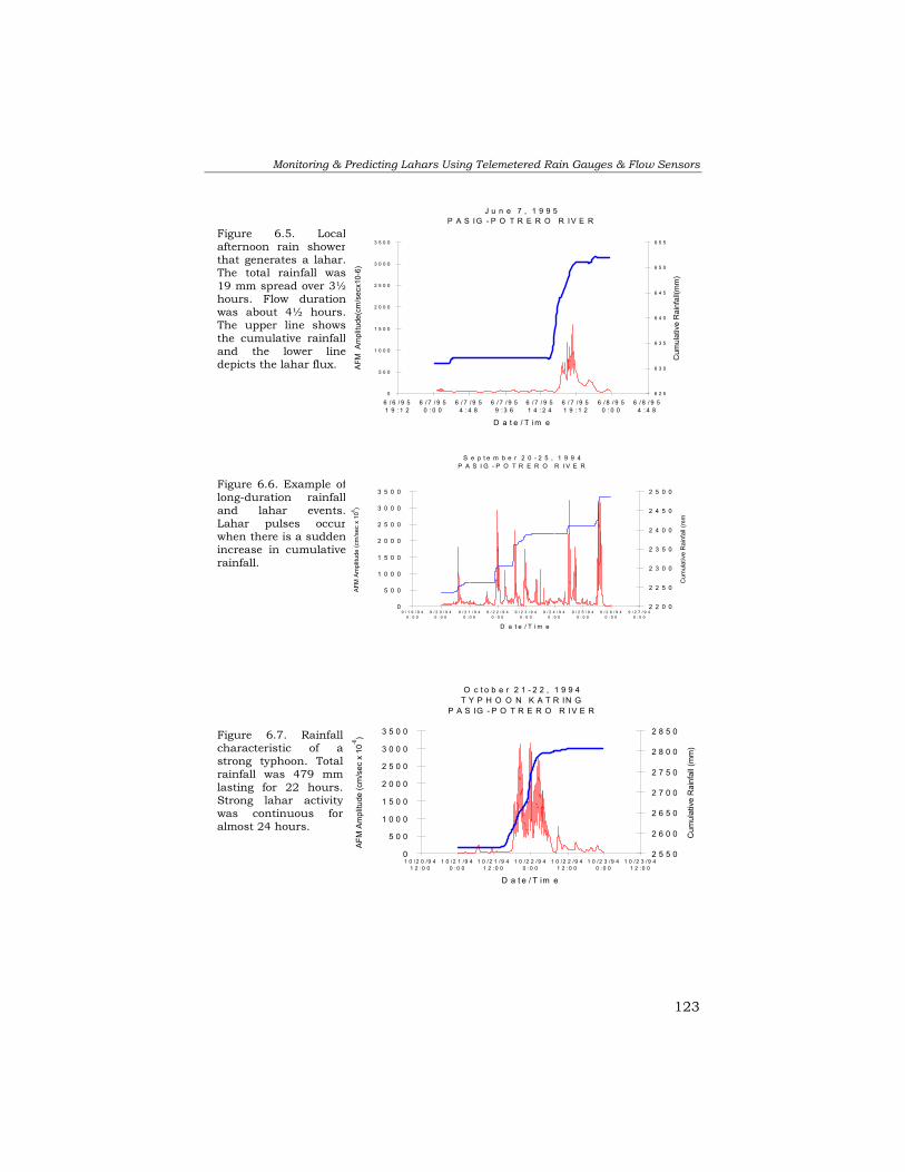
Monitoring & Predicting Lahars Using Telemetered Rain Gauges & Flow Sensors
123
O c t o b e r 2 1 - 2 2 , 1 9 9 4T Y P H O O N K A T R IN G
P A S IG - P O T R E R O R IV E R
0
5 0 0
1 0 0 0
1 5 0 0
2 0 0 0
2 5 0 0
3 0 0 0
3 5 0 0
1 0 /2 0 /9 41 2 :0 0
1 0 /2 1 /9 40 :0 0
1 0 /2 1 /9 41 2 :0 0
1 0 /2 2 /9 40 :0 0
1 0 /2 2 /9 41 2 :0 0
1 0 /2 3 /9 40 :0 0
1 0 /2 3 /9 41 2 :0 0
D a t e / T im e
AFM
Am
plitu
de (c
m/s
ec x
10-6
)
2 5 5 0
2 6 0 0
2 6 5 0
2 7 0 0
2 7 5 0
2 8 0 0
2 8 5 0
Cum
ulat
ive
Rai
nfal
l (m
m)
Figure 6.7. Rainfallcharacteristic of astrong typhoon. Totalrainfall was 479 mmlasting for 22 hours.Strong lahar activitywas continuous foralmost 24 hours.
Figure 6.5. Localafternoon rain showerthat generates a lahar.The total rainfall was19 mm spread over 3½hours. Flow durationwas about 4½ hours.The upper line showsthe cumulative rainfalland the lower linedepicts the lahar flux.
J u n e 7 , 1 9 9 5P A S IG - P O T R E R O R I V E R
0
5 0 0
1 0 0 0
1 5 0 0
2 0 0 0
2 5 0 0
3 0 0 0
3 5 0 0
6 / 6 / 9 51 9 : 1 2
6 / 7 / 9 50 : 0 0
6 / 7 / 9 54 : 4 8
6 / 7 / 9 59 : 3 6
6 / 7 / 9 51 4 : 2 4
6 / 7 / 9 51 9 : 1 2
6 / 8 / 9 50 : 0 0
6 / 8 / 9 54 : 4 8
D a t e / T im e
AFM
Am
plitu
de(c
m/s
ecx1
0-6)
6 2 5
6 3 0
6 3 5
6 4 0
6 4 5
6 5 0
6 5 5
Cum
ulat
ive
Rai
nfal
l(mm
)
Figure 6.6. Example oflong-duration rainfalland lahar events.Lahar pulses occurwhen there is a suddenincrease in cumulativerainfall.
S e p t e m b e r 2 0 - 2 5 , 1 9 9 4P A S I G - P O T R E R O R I V E R
0
5 0 0
1 0 0 0
1 5 0 0
2 0 0 0
2 5 0 0
3 0 0 0
3 5 0 0
9 / 1 9 / 9 40 : 0 0
9 / 2 0 / 9 40 : 0 0
9 / 2 1 / 9 40 : 0 0
9 / 2 2 / 9 40 : 0 0
9 / 2 3 / 9 40 : 0 0
9 / 2 4 / 9 40 : 0 0
9 / 2 5 / 9 40 : 0 0
9 / 2 6 / 9 40 : 0 0
9 / 2 7 / 9 40 : 0 0
D a t e / T i m e
AFM
Am
plitu
de (c
m/s
ec x
10-6
)
2 2 0 0
2 2 5 0
2 3 0 0
2 3 5 0
2 4 0 0
2 4 5 0
2 5 0 0
Cum
ulat
ive
Rai
nfal
l (m
m)

Chapter 6
124
Figure 6.9. Box plot diagram of different rainfall magnitudes that triggered lahars. Seetext for further explanation.
S e p t e m b e r 2 0 - 2 5 , 1 9 9 4P A S I G - P O T R E R O R I V E R
0
5 0 0
1 0 0 0
1 5 0 0
2 0 0 0
2 5 0 0
3 0 0 0
3 5 0 0
0 9 / 1 9 / 94 0 : 0 0
0 9 / 2 0 / 94 0 : 0 0
0 9 / 2 1 / 94 0 : 0 0
0 9 / 2 2 / 94 0 : 0 0
0 9 / 2 3 / 94 0 : 0 0
0 9 / 2 4 / 94 0 : 0 0
0 9 / 2 5 / 94 0 : 0 0
0 9 / 2 6 / 94 0 : 0 0
0 9 / 2 7 / 94 0 : 0 0
D a t e / T i m e
AFM
Am
plitu
de (c
m/s
ec x
10-6
)
2 2 0 0
2 2 5 0
2 3 0 0
2 3 5 0
2 4 0 0
2 4 5 0
2 5 0 0
Cum
ulat
ive
Rai
nfal
l (m
m)
Figure 6.8. Cumulative rainfall of the “siyam-siyam” type (see Chapter 3) andcorresponding flow data of multiple lahar events.

Monitoring & Predicting Lahars Using Telemetered Rain Gauges & Flow Sensors
125
The extreme values were statistically treated as outliers but in reality they are mostly the low-intensity longer-duration rainfalls. The figure also depicts how much variation in rainfall magnitude can be expected. The total amount of rainfall before a lahar is initiated is a function of intensity and duration. The lower tail-ends of the range are generally consistent, showing about 3 mm of rainfall. These events are the low-intensity and longer-duration rainfall occurrences. Extreme values above the range (shown in horizontal bar) were several orders of magnitude away from the mean rainfall magnitude. 6.7.2 Rainfall intensity-duration relationships Another way of obtaining rainfall-lahar thresholds is by correlating the rainfall intensity and duration with the lahar occurrence. From the envelopes of lahar thresholds, a power curve fitting is the most suitable correlation trend for the rainfall-lahar threshold. The power fitting regression has been used in several studies (Rodolfo and Arguden, 1991; Tungol and Regalado, 1996; Lavigne et al., 1998). The curve is characterized by the following equation:
bcDI −=
where I = rainfall intensity D = rainfall duration c and b are constants.
The resulting power fitting from all the data is negatively correlated. This would mean that, in order to trigger a lahar, a higher rainfall intensity is required for a shorter rainfall duration and a longer rainfall duration is required for a lower rainfall intensity. This is not surprising since it is normal for the relationships to behave in this way. What is remarkable is the very low rainfall that is required to trigger lahars. 6.7.2.1 Average yearly thresholds Due to extreme data values that represented both rainfall- and non rainfall triggered lahars, only the events that triggered lahars were considered in order to limit the huge deviations in the threshold values. About 286 rainfall-triggered lahar data points were considered, and plotted as shown in Figure 6.10. A power curve was used for the regression analysis. The relationship between rainfall intensity and duration is:
663.0284.3 −= DI
This relationship is an approximation of thresholds to initiate lahars. This would mean that at an average, a minimum of 0.33 mm/min rainfall intensity with a minimum duration of 30 min or 0.22 mm/min
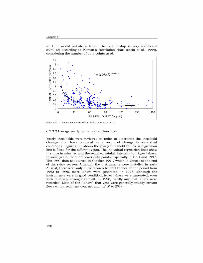
Chapter 6
126
in 1 hr would initiate a lahar. The relationship is very significant (r2=0.18) according to Pierson´s correlation chart (Stein et al., 1999), considering the number of data points used.
6.7.2.2 Average yearly rainfall-lahar thresholds Yearly thresholds were reviewed in order to determine the threshold changes that have occurred as a result of change in watershed conditions. Figure 6.11 shows the yearly threshold values. A regression line is fitted for the different years. The individual regression lines show the time in minutes and the required rainfall intensity to trigger lahars. In some years, there are fewer data points, especially in 1991 and 1997. The 1991 data set started in October 1991, which is almost at the end of the rainy season. Although the instruments were installed in early August, there were only a few records before October. In the period from 1992 to 1996, more lahars were generated. In 1997, although the instruments were in good condition, fewer lahars were generated, even with relatively stronger rainfall. In 1998, hardly any real lahars were recorded. Most of the “lahars” that year were generally muddy stream flows with a sediment concentration of 10 to 20%.
I = 3.284D -0.6443
0
0.2
0.4
0.6
0.8
1
1.2
1.4
1.6
1.8
2
2.2
0 30 60 90 120 150 180RAINFALL DURATION (min)
RAI
NFA
LL IN
TEN
SITY
(mm
/min
)
Figure 6.10. Seven-year data of rainfall triggered lahars.

Monitoring & Predicting Lahars Using Telemetered Rain Gauges & Flow Sensors
127
I = 3.2164D -0.7397
0
0.5
1
1.5
2
0 30 60 90 120 150 180RAINFALL DURATION (min)
RAI
NFA
LL IN
TEN
SITY
(mm
/min
) YEAR 1991
I = 2.5223D -0.579
0
0.5
1
1.5
2
0 30 60 90 120 150 180RAINFALL DURATION (min)
RAI
NFA
LL IN
TEN
SITY
(mm
/min
) YEAR 1992
I = 10.887D -1.058
0
0.5
1
1.5
2
0 30 60 90 120 150 180RAINFALL DURATION (min)
RAI
NFA
LL IN
TEN
SITY
(mm
/min
) YEAR 1993
I = 6.4103D -0.8652
0
0.5
1
1.5
2
0 30 60 90 120 150 180RAINFALL DURATION (min)
RAI
NFA
LL IN
TEN
SITY
(mm
/min
) YEAR 1994
I = 3.2182D -0.6078
0
0.5
1
1.5
2
0 30 60 90 120 150 180RAINFALL DURATION (min)
RAI
NFA
LL IN
TEN
SITY
(mm
/min
) YEAR 1995
I = 1.8278D -0.4503
0
0.5
1
1.5
2
0 30 60 90 120 150 180RAINFALL DURATION (min)
RAI
NFA
LL IN
TEN
SITY
(mm
/min
) YEAR 1996
I = 14.523D -0.9114
0
0.5
1
1.5
2
0 30 60 90 120 150 180RAINFALL DURATION (min)
RAI
NFA
LL IN
TEN
SITY
(mm
/min
) YEAR 1997
Figure 6.11. Yearly relationships of rainfall intensity (I) and rainfall duration (D) that triggeredlahars. The corresponding equations are shown in each plot.

Chapter 6
128
Interesting trends appear when comparing the different thresholds of the different years. The equations presented in Figure 6.11 were used to generate threshold levels of rainfall intensity and duration that would be required to trigger lahars. The results are displayed in Figure 6.12. The graph plots the threshold values in different rainfall durations, i.e., 15, 30, 45, 60 and 90 minutes. From this figure it can be deduced that the threshold amounts vary through time. It is logical to expect that the threshold value will increase each season because each year the source materials in the watershed are decreasing. In the Pasig watershed, the physical conditions changed significantly each year, causing the triggering thresholds to show variable trends. It can be observed from the graphs that in 1991 smaller rainfall intensities and duration were needed to trigger lahars. This condition is to be expected since erodible source sediments were abundant and a dense gulley network was formed which made erosion quite efficient. However, immediately after the eruption the moisture condition of the pyroclastic flow materials was still rather low. Consequently more time was needed for the deposits to become saturated before the lahars could be initiated. This condition was also observed after a new secondary pyroclastic flow had occurred. The 1991 threshold data were only available from October, without any significant data at the start of the rainy season, thus making the calculated threshold less reliable.
Figure 6.12. A lahar-triggering threshold predictive model based on the trend lines onrainfall intensity and duration. The thresholds differ each year as a result of dynamicwatershed changes, i.e., stream piracy. Eventually, higher thresholds are required as thewatershed stabilizes.
0
0.2
0.4
0.6
0.8
1
1.2
1991 1992 1993 1994 1995 1996 1997YEAR
RAI
NFA
LL IN
TEN
SITY
(mm
/min
)
15min 30min 45min 60min 90min
Monitoring & Predicting Lahars Using Telemetered Rain Gauges & Flow Sensors
129
The 1992 values show that a higher rainfall threshold was required to trigger lahars. The relative increase in threshold values is in the order of 25 to 35% for a rainfall duration of 30 to 60 minutes. In 1993 there was a major transition in the Pasig-Sacobia watershed owing to the secondary explosion of 6 October, which caused the capture of 20 km2
of the upper Sacobia watershed by the Pasig River. This resulted in substantially reduced lahar magnitude in the Sacobia River and a remarkable increased lahar hazard in the Pasig River. This major change is not clearly reflected in the calculated threshold values for 1993 since the event occurred almost at the end of the rainy season. The 1993 graph shows an increase in threshold values for shorter rainfall duration only (5 to 30 min). From 1994 to 1997, there is a slight progressive increase in threshold levels as the watershed progressively “recovers” and sediment entrainment becomes less effective. This can be a function of depleting source sediments and valley widening. Wide U-shaped valley floors are less susceptible to lateral erosion during small flows. The only effective way to erode is during a large flows when lateral erosion and undercutting play a major role. Thus, this requires a higher rainfall magnitude before lateral erosion begins. In this study, the linear relationships of rainfall intensity and duration are not very high but a good range could be established for the yearly and the overall plots combined for the seven years. We may expect that rainfall-lahar trigger values will vary each year as a result of the changing morphology of the watershed. The data showed that no good linear relationship could be established. 6.8 Lahar rheology determination using acoustic flow sensor The acoustic flow monitoring (AFM) system not only provides information related to the timing of lahar events, it can also provide useful information on the lahar type. The difference between the strength of the low and high band acoustic signals can give a general estimation of the sediment concentration in the flow (Hardley and Lahusen, 1993; Lavigne et al., 1998). At Merapi, moderately sized lahar events have signals of about 500 AFU. During bigger flows, debris flows can have a signal of about 1100 AFU while hyperconcentrated flows yield signal of 350 AFU. The difference between low and high band signals can be fivefold for debris flows. Diluted lahars show little difference in the low and high band signal (Lavigne at al., 1998). At Pinatubo, several observations of active lahars were carried out in the field, which were correlated with the corresponding flow sensor data. Most of these observations were done along the Sacobia and Pasig lahar channels.

Chapter 6
130
Depending on the type of flow, either one of the signals dominates. Debris flows produce more low frequency signals; hence this signal dominates the low band signal when this type of flow occurs. On the other hand, during diluted hyperconcentrated flows to muddy stream flows, the high band signal records higher values than the low band signal. In order to establish the relationships between the two band signals with the types of lahar flow, a simple direct subtraction of the two band signals was made. Since low band signals are dominant during several lahar events, we use the low band signal as a minuend and the high band as a subtrahend. In this regard, positive high values are expected for debris flow events. For example, 1500 AFU (low band) minus 100 AFU (high band) will give a difference of 1400 AFU. This example is considered as debris flow, since low band values are dominant. The larger the AFU difference, the more sediment concentration the debris flow or hyperconcentrated flow will have. On the other hand, during diluted hyperconcentrated flow to muddy stream flow, the values of the high frequency band are greater than those of the low band. For example, 100 AFU (low band) minus 500 AFU (high band) will give negative 400 AFU. At Mt. Pinatubo, high-density debris flows can have a difference of 2,500 AFU between low and high band signals, while for muddy stream flows the difference can be -500. A lahar flow discharge of 200 m3/s can have an acoustic signal of 1,200 AFU and a flow with a discharge of 500 m3/s about 2,000 AFU. Figure 6.13 illustrates the average difference in the acoustic signals of several lahar events plotted chronologically for seven years. Each dot represents the average difference between low and high band signals of one single event. It can be deduced that during the initial years of lahars the events generated were mostly debris flows or hyperconcentrated flows. In the initial years, from 1991 and up to the stream capture incidents (October 1993), the average flux difference is not very high, in the order of 300 to 400. Most of these lahars are considered events of moderate size. After the capture in October 1993, subsequent lahars were remarkably large, in terms not only of magnitude but also of difference in low and high band signals, indicating that most lahars were debris flows. Most of the observed large flows (debris and hyperconcentrated flows) have associated acoustic flow values with large discrepancies between the low and high band signals. The difference is in the order of at least 300 AFU and even greater for larger flows. In 1997, lahar flows were more diluted, resulting in high band dominated signals.

Monitoring & Predicting Lahars Using Telemetered Rain Gauges & Flow Sensors
131
6.9 Lahar discharge measurements Data from the acoustic flow sensors were correlated with observed lahars. Most observations were done in the initial years (1991 and 1992) at Sacobia and on some occasions at Pasig. Some events were fully observed, from the front right up to the tail of the flow. These flows were generally small events lasting only a few hours. It is hard to document the full event of large flows because they may last for a day or even more. Field calculation of active lahar discharge has a number of inherent uncertainties. A great uncertainty lies in the measurement of the flow depth of relatively large flows. Lahars are very erosive, thus during flows streambed profile can change significantly, resulting in some uncertainty in the measurement of volume discharge. As regards relatively small flows, there may be some measurable objects that could lead to a better estimation. These are the dunes and anti-dunes of flow
ACOUSTIC FLUX DIFFERENCE BETWEEN LOW AND HIGH FREQUENCY SIGNALS OF LAHAR EVENTS
-1000
-500
0
500
1000
1500
2000
2500
3000
1991
1992
1992
1993
1994
1994
1994
1994
1994
1994
1995
1995
1995
1996
1996
1997
1997
1997
YEAR
AVE
RA
GE
FLU
X D
IFFE
REN
CE
Figure 6.12. Lahar events (red dots) showing the acoustic signal strenght difference(low vs. high frequency) for a period of 8 years following the 1991 eruption. Eventsabove the zero line are low frequency dominated signals, while events that havenegative values are signals dominated by high frequency. Points with a value above100 are considered debris- and hyperconcentrated-dominated flows, while eventsbelow negative 100 flux are muddy to watery flows.
Figure 6.13. Lahar events (in small dots) showing the acoustic flow signal difference (lowfrequency band minus high band) for the period of seven years. Events above the zeroline are low band dominated signals, while events with negative values are dominated byhigh band signals. Points with a value above +100 are considered debris andhyperconcentrated flows, while events below -100 are muddy to watery flows.
Chapter 6
132
and the presence of rolling boulders. In general, since the estimation of discharge is mostly visual, subjectivity plays a role. Since 1997 lahar activity has greatly diminished, mainly due to the depletion of source materials. Heavy rainfall during a typhoon in September 1998 only produced muddy stream flow with a maximum 25% sediment volumetric ratio. Despite the strong rainfall, no debris or hyperconcentrated flows were observed. Hayes (1999) has correlated discharge (m3/s) with acoustic flow monitoring values (AFM units in cm/s x 10-6) of low band signals. These flows generally range from muddy stream flow to small flow lahars at Pasig River in 1997 and 1998. A correlation equation of Q=0.34AFM with r=0.85 was obtained. The flow observations were mostly below 20 m3/s. An acoustic reading of 100 units roughly corresponds to a discharge of 35 m3/s. Tungol and Regalado (1996) correlated the debris flows and hyperconcentrated flows at the Sacobia channel with the AFM values in July and August 1992. They obtained the relationship of Q=0.24AFM with a correlation coefficient of r=0.76. Lahar discharge ranged from tens to 600 m3/s. The relationship tends to be exponential for higher flow sensor amplitude (>2,000) and high discharge. Figure 6.14 displays the lahar discharge and the corresponding flow sensor values (low band) observed at the Pasig channel during a 12-hour period on 29 August 1992. Although there are some gaps in the discharge estimation, the lahar was observed from the start of the initial flow at 11:45 hrs to the period of normal stream flow with a discharge of no more than 10 m3/s and acoustic signals of less than 100 units. Acoustic signals above 300 have at least 250 m3/s discharge and these are lahars (debris to hyperconcentrated flows). The rheology of flow changed from lahar (from 12:00 hrs to 14:30 hrs) to transitional muddy stream flow (14:30 hrs to 16:00 hrs) and back again to lahar (mostly hot debris flow). Acoustic flow data will give an estimate of the type of flow that can be expected in the channel even without direct observation in the field. Estimating the lahar discharge purely by correlating the acoustic flow signals will result in a very rough estimate of the flow, as presented by Tungol and Regalado (1996) and Hayes (1999).

Monitoring & Predicting Lahars Using Telemetered Rain Gauges & Flow Sensors
133
6.10 Discussion and conclusions This chapter discussed the use of telemetered rain gauge and flow sensor data to define the relationships between rainfall and lahar occurrences. In some cases, the flow sensor signals were used to estimate the magnitude and rheology of lahar flows. Several field observations were conducted to correlate the rain gauge and flow sensor data. The major advantage of the telemetry system is that it can record data continuously from many field stations in real time, which is vital for lahar warning. Data are received in digital format and can be used directly to model rainfall-lahar thresholds, magnitude and duration of lahar flows, and in estimating the rheology of lahars flows. However, some data gaps were inevitable when some instruments ceased operation or when transmitted data was badly affected by radio noise. This system also has some drawbacks, such as: a) Rain gauges must be positioned on highly elevated areas where
antennas can have a line-of-sight to the base station for data transmission, however in many cases these sites are also prone to lightning strikes;
b) Flow sensors are positioned near the active lahar channels to maximize the signal produced by vibrations during lahar flows. In some cases channel erosion can endanger the instruments, which might be lost or should be relocated, which makes the data difficult to compare with previous records;
Figure 6.14. Record of acoustic flow difference (low minus high band signal strengthshown in dots) and corresponding lahar discharge (solid line) at the Pasig channel. Flowsignal difference below 100 is considered as muddy stream flow to dilutedhyperconcentrated flow.
-2000-1500-1000-500
0500
10001500200025003000
DATE AND TIME OF OBSERVATION
Acou
stic
Flu
x D
iffer
ence
(L
ow -
Hig
h Fr
eq.)
8/29/199209:21
8/29/199211:45
8/29/199214:09
8/29/199216:33
8/29/199218:57
8/29/199221:21
Chapter 6
134
c) The sensors are powered by batteries, which are recharged by a solar panel. Heavy ash fall or several cloudy days may lead to depletion of the batteries and malfunctioning of the system;
d) Telemetry data are transmitted using radio frequencies, which may sometimes cause problems due to radio interferences leading to strongly distorted recorded data.
In total, six rain gauges and seven flow sensors were installed on the upper slopes of Mt. Pinatubo volcano. Rainfall data are transmitted per 1 mm of rainfall, while flow sensor data are send every minute when a threshold value is met. Flow sensors record vibration using acoustic signals in three frequencies, i.e., low (10-100 Hz), high (100-300 Hz), and broad-band (10-300 Hz). A huge amount of data was collected over a span of 7.5 years. About 430 lahar events were recorded but only about 286 events could be used in the analysis of the rainfall-lahar threshold relation due to missing rainfall record as a result of sensor malfunctioning. Although the long-term erosion decay curve included a range of uncertainty, the effect of stream capture has made the prediction to deviate in some years from the forecasted values. In the first two years (1991 and 1992) of the studied period, there was a Pacific-wide El Niño Southern Oscillation (ENSO) event. This caused the southwest monsoon to arrive late and last for a shorter period, resulting in less rain in these particular years. Following the El Niño event, in 1993 and 1994 the occurrence of heavy rainfall events and typhoons and the effect of the stream capture enhanced the accelerated erosion significantly and resulted in more lahar events. From 1995 to 1997, however, the number of actual lahar events was significantly lower than the predicted one. The presence of high mountains significantly affects the rainfall variation over the Mt. Pinatubo area. It leads to some localized convection cells with intense rainfall that is sometimes not recorded by the rainfall network. Therefore lahar occurrences might be recorded with very low triggering rainfall values measured in the rain gauges. In the opposite case, extreme high rainfall values may be concentrated in the area of the rain gauge itself, whereas no lahar is recorded by the flow sensors. The installed rain gauges and flow sensors were an important tool in lahar warning. The flow sensors gave about 30 minutes' to an hour's lead-time before the lahars were detected at the first lahar watch point. It was then about an hour or more before they reached the community downstream. These systems were successful in issuing warnings of lahars and have been extensively used in the Pinatubo area.

Monitoring & Predicting Lahars Using Telemetered Rain Gauges & Flow Sensors
135
Rainfall events that triggered lahars in the period from 1991 to 1997 were presented using box plots as shown in Figure 6.9 and the results suggest that strong variations of rainfall magnitude have triggered lahars. On an average, a rainfall magnitude of 13 mm was sufficient to trigger lahars. The lahar-triggering rainfall amounts varied significantly from year to year as a result of changing morphological conditions in the watersheds. Rainfall intensity-duration relationships were used to determine the rainfall-lahar threshold using a power function. A power function gives a better correlation, as was also proven in the case of other volcanoes. The average threshold for the seven-year data was represented by the equation I=3.284D-0.663 (I = rainfall intensity and D = rainfall duration). This means that on the average, a rainfall intensity of 0.33 mm/min with duration of 30 minutes (or 0.22 mm/min in 1 hour) is required to trigger lahars. Yearly average rainfall-lahar thresholds vary significantly each year as presented in Figure 6.11. Higher rainfall intensity and duration was required to trigger lahars in subsequent years, ranging from 0.3 mm/min for half an hour in the period from 1991 to 1993 up to 0.4 to 0.6 mm/min in 30 minutes in the period from 1995 to 1997. These thresholds are significantly lower than those reported for the Mayon and Merapi volcanoes. From the flow sensor data recorded in three different frequencies it was possible to extract a number of relations. The magnitude and the duration of lahar flows in 1992 for the Sacobia river can be estimated by the relationship Q=0.24AFU (AFU = Acoustic flow units) (Tungol and Regalado, 1996). Hayes (1999) presented the relationship of Q=0.34AFU for muddy stream flows along the Pasig river. The established equations can be site or channel specific since the distance of the sensor to the active lahar channel can influence the sensitivity of the sensor and likewise the channel configuration can change after major lahar events. The data from the three frequencies of the flow sensors can also be used to estimate the rheological condition of lahars, and allow differentiating between lahars (debris flows or hyperconcentrated flows) and muddy stream flows. Debris flows produce low frequency vibrations while muddy stream flows generate high frequency ones. The difference between the values recorded in the low band and high band (Low minus High band) allow differentiating between the two types. An average flux difference of 100 AFU is typical for debris flows and hyperconcentrated flows while a difference of –100AFU is typical for muddy stream flows. The seven-year acoustic flow data suggest that debris flows were most prominant in the period from 1991 to early 1996, whereas after this period the lahars evolved into more diluted flows. The flow sensor data also allowed to determine the relative timing of the stream capture event of Pasig and Sacobia in October 1993, resulting in a sudden shift of lahar flow magnitude from the Sacobia to the Pasig River.

Chapter 6
136

The Use of Portable Rainfall Simulator for Erosion Estimation
137
Chapter 7: The Use of a Portable Rainfall Simulator for Erosion Estimation in Pyroclastic Flow Deposits 7.1 Introduction Most of the current understanding in quantitative soil erosion research was formulated using various rainfall simulators (Bubenzer, 1979). The advantage of using rainfall simulators is that the characteristics of the raindrops plus the intensity can be controlled under certain conditions. The fall height, the kinetic energy of rainfall, and the size, frequency and spacing of the raindrops can all be adjusted (Onstad et al., 1981). In terms of sophistication, rainfall simulators come with a variety of features and in a variety of sizes, ranging from a small portable set-up to large laboratory-based systems. Most rainfall simulators have standard features, such as the amount and intensity of rainfall that can be regulated. In this study, a simple portable rainfall simulator was used. The small simulator was ideal in the study area because of the poor accessibility of the site and the need to do in situ rainfall simulations on the different types of deposits. 7.2 Objectives and methods The objective of this chapter is to study the runoff and erosion of the different in situ lahar source sediments under simulated rainfall and under different slope conditions. Research has been conducted in correlating the rainfall magnitudes and intensities with lahar discharge at catchment scale, both instrumentally and with field observations under natural rainfall conditions. However, in order to understand the response of various deposits under different rainfall intensities in detail, more detailed field measurements were required. The different physical properties and characteristics of the deposits that influence erosion and runoff were studied. The results of the experiments will be used semi-quantitatively and qualitatively in the erosion modeling that will be treated in Chapter 8. The resulting data are only indicative of relative erosion and should not be treated as absolute values. To carry out these in situ experiments, a rainfall simulator was operated in the field under different rainfall intensities (2, 4, 6, and 12 mm/min). Field plots were prepared with different slope gradients of 20, 40, 60, 80

Chapter 7
138
and 100%. The physical properties of the sediments, such as soil strength and grain size distribution, were also determined in order to study the effects of these parameters on runoff and erodibility. Also erosion pins were set up in the field in a mini-catchment. Basically an erosion pin is a steel bar, about half a meter long, which is driven into the soil, leaving only a few millimeters unburied. Erosion can be monitored by measuring how much of the bar becomes exposed. Unfortunately, since the measurements were made during several months of the dry season, there was not enough strong rainfall to trigger substantial erosion during this period. 7.3 Characteristics of lahar source materials One of the main aspects in the study of erosion is to determine the physical characteristics of the different deposits that contribute to the development of lahar flows. The source sediments of Mt. Pinatubo lahars are the following material types (in order of importance): • Pyroclastic flow materials deposited during the 1991 eruption • Pre-eruption pyroclastic flow materials • Local lahar deposits • Volcanic ash Analysis of the lahar deposits produced in different years suggests an evolution in their source sediments. This is especially clear in the Pasig channel of the study area. In 1991, the lahar source sediments were primary pyroclastic flows and tephra fall. In the succeeding years, as tephra fall material became depleted, the pyroclastic flows were the biggest source of lahar sediments. Starting from the year 1994, deep gullies evolved dissecting pre-1991 eruption deposits, which were assimilated into the new lahars. Lake breakout events also scoured tremendous amounts of old materials. Tephra fall is the most widely distributed deposit, blanketing about 2,000 km2. Its contribution to lahars was only significant in the first few years. Some lahars that had traveled short distances were redeposited in the upper watershed and have the potential to be remobilized. They occur only along valley floors and are sometimes deposited on top of the new pyroclastic flow deposits. They are generally limited in occurrence in terms of both space and volume. These types of lahars are poorly sorted and are still rich in fines in comparison with hyperconcentrated flows and lahars that have traveled over a greater distance.

The Use of Portable Rainfall Simulator for Erosion Estimation
139
There are two kinds of pyroclastic flows that contribute to the lahar sediments. These are the old pre-1991 and the 1991 eruption pyroclastic flows. In the field, these two types of deposits are basically similar in terms of sedimentologic properties. Most of the pre-1991 pyroclastic flow deposits are at least 500 to a few thousand years old. As they have no soil development, they are difficult to distinguish in the field from recent ones. 7.3.1 Grain size distribution Lahars at Mt. Pinatubo basically consist of remobilized 1991 pyroclastic flow deposits. As mentioned in Chapter 4, these deposits were emplaced very hot (around 600°C), with almost no moisture content, no cohesion or shear strength, and behaving like dry powder. Fresh deposits measured using a 0.5 m thermometer probe a few months after the eruption showed surface temperatures of about 230°C. Deposits of more than 100 m thick will maintain their high temperatures since they are poor conductors of heat and thus temperature dissipation is slow. These high temperatures were sustained for several years, as witnessed by the production of hot lahars observed even during some lahar events in 1997. The 1991 pyroclastic flow deposits have massive structures and are matrix-rich and sand-size sediment supported; an individual depositional event can be several meters thick. They have poor sorting since they are deposited en masse, without any time for sorting. The 1991 pyroclastic flows can be further classified based on their process of emplacement, that is, primary and secondary (remobilized primary) pyroclastic flows. The two types of deposits have a similar structure and grain size distribution. The only difference is the smaller amount of fines present in the secondary pyroclastic flows because they have been removed by elutriations (ash clouds). Other than that, they can also be distinguished using a magnetometer, based on the principle that magnetic minerals tend to align to the magnetic North when deposited above the melting point, which surpassed the emplacement temperature of the primary pyroclastic flows. In the case of secondary pyroclastic flows, inconsistent thermo-remanent polarity of the clasts is exhibited due to lower emplacement temperatures (Torres et al., 1996). Scott et al. (1996) and Torres et al. (1996) reported the characterization of the primary and secondary deposits in detail. The 1991 deposits generally consist of a sandy matrix with median grain sizes of 0.25 to 1 mm and between 60 to 90% sediment in weight. Results of detailed grain size analyses of the primary and secondary pyroclastic flow deposits are shown in Figure 7.1 (after Torres et al., 1996).

Chapter 7
140
From the figures, it can be observed that primary and secondary pyroclastic flows have almost similar grain size distribution. Compared with a deposit, active hyperconcentrated flows are rich in fine sand and silt content. Lake breakout flood and debris flows are rich in coarser fractions. Tephra falls, due to their coarse-grained composition, are uncompacted and highly erodible.
Several grain size analyses were also done using sampled active lahar flows and deposits. The median grain sizes of these deposits are displayed in Figure 7.2
Figure 7.1. Grain size plots of primary and secondary pyroclastic flow deposits(ignimbrite), as presented by Torres et al. (1996). There is no great distinction betweenthe two types of pyroclastic flow deposits in terms of sedimentary structures and generalgrain sizes. However, there is a slight decrease in fines in the secondary deposits sincethe remobilisation turns some fines into ash cloud (as elutriates).
99
95
40
50
60
70
80
90
5
10
20
30
24816 1/81/41/21 1/16
-3-4 0-1-2 +3 +4+2+1PHI UNITS
MILIMITERS
PRIMARY PYROCLASTICFLOW DEPOSITS
MILIMITERS99
95
40
50
60
70
80
90
5
10
20
30
24816 1/81/41/21 1/16
-3-4 0-1-2 +3 +4+2+1PHI UNITS
SECONDARY PYROCLASTICFLOW DEPOSITS

The Use of Portable Rainfall Simulator for Erosion Estimation
141
Median grain size of lahars (debris flow and hyperconcentrated flow) are mostly in the range of 0.5 to 2 mm (-1 to 1 phi) (medium to coarse sand). Primary and secondary pyroclastic flow deposits have a median grain size range of 0.25 to 1 mm (medium sand). All of these deposits are sand-rich, with lahars having slightly less finer sediments (silt and clay) because they are washed away during the flow. 7.3.2 Shear strength Soil strength and texture have a direct influence on the erodibility of soil. They determine how cohesive and compacted the soil is. In this study, a vane shear meter (Torvane) was used to study the soil strength whenever possible. Field measurements were conducted in different deposits. To compare the behavior of deposits during dry and wet states, conditions of deposits were measured before and after conducting rainfall simulations. Table 7.1 shows the average shear strength of the different deposits, respectively. It can be noted that the shear strength under dry conditions can be twice as much as during wet conditions. To give a general idea of how the deposits behave, the value of 1 kilopascal (kPa) in the graph is a loose sand (comparable to tilled agricultural soil). Thus, wet deposits have almost no inherent shear strength. This is important in the rainfall runoff simulations on soils, since the structure of this type of deposit is prone to collapse when saturated with rain.
Figure 7.2. Median grain size distribution of a pyroclastic flow and several lahars (activeand deposited lahars) taken from various studies and from this study. Codes in the y-axis are: PF=pyroclastic flow, HF=hyperconcentrated flow and DF=debris flow.
MEDIAN GRAIN SIZE OF PYROCLASTIC FLOW AND ACTIVE LAHARS
-4 -3 -2 -1 0 1 2 3 4
DFDFDFDFDFDFDFDFDFDFDFDFDFHFHFHFHFHFHFHFHFHFHFHFPF
TYPE
OF
DEP
OSI
T
DIAMETER IN PHI
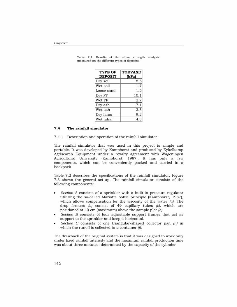
Chapter 7
142
TYPE OF DEPOSIT
TORVANE (kPa)
Dry soil 8.5 Wet soil 1.7 Loose sand 1.2 Dry PF 10.1 Wet PF 2.7 Dry ash 7.1 Wet ash 3.5 Dry lahar 9.2 Wet lahar 4.3
7.4 The rainfall simulator 7.4.1 Description and operation of the rainfall simulator The rainfall simulator that was used in this project is simple and portable. It was developed by Kamphorst and produced by Eykelkamp Agrisearch Equipment under a royalty agreement with Wageningen Agricultural University (Kamphorst, 1987). It has only a few components, which can be conveniently packed and carried in a backpack. Table 7.2 describes the specifications of the rainfall simulator. Figure 7.3 shows the general set-up. The rainfall simulator consists of the following components: • Section A consists of a sprinkler with a built-in pressure regulator
utilizing the so-called Mariotte bottle principle (Kamphorst, 1987), which allows compensation for the viscosity of the water (a). The drop formers (e) consist of 49 capillary tubes (c), which are positioned at 40 cm (maximum) above the sample plot (b).
• Section B consists of four adjustable support frames that act as support to the sprinkler and keep it horizontal.
• Section C consists of one triangular-shaped collector pan (h) in which the runoff is collected in a container (i).
The drawback of the original system is that it was designed to work only under fixed rainfall intensity and the maximum rainfall production time was about three minutes, determined by the capacity of the cylinder
Table 7.1. Results of the shear strength analysismeasured on the different types of deposits.

The Use of Portable Rainfall Simulator for Erosion Estimation
143
tank (a). In order to have uniformly comparable measurements of different soil types in the world, the system was also designed to work only on a slope of about 20%. The procedure for rainfall simulations is as follows: A 25 x 25 cm plot (g) with a slope of 20% is prepared on the ground. The whole system is set up over the plot but initially without water in the sprinkle section. The frame of the sprinkler system is then leveled horizontally using a simple bubble-type leveling system. The sprinkler system is placed upside down and water is poured in; a funnel is used to pour the water in (f) while at the other end (d) the cork is still plugged in. After the cylinder is filled with water, the cork is re-plugged at the opening (f) and the sprinkler system is again turned right side up. In this position no water comes out because it is still in a vacuum and the system is watertight. Rainfall simulation is started when the cork is removed from the cylinder head. During the simulation the sprinkler head is moved horizontally from side to side in order to distribute the water drops evenly onto the plot. When the rainfall simulation is finished, the accumulated sample is analyzed.
Table 7.2. Specifications of the rainfall simulator.
Magnitude of rain shower 10 mm Duration of rain shower 3 min Intensity of rain shower 6 mm/min Fall height of drops at top of slope 375 mm Fall height of drops at bottom of slope
425 mm
Average fall height of drops 400 mm Diameter of drops 5.9 mm Mass of drops 0.106 g Number of capillary tubes 49 pieces Kinetic energy of event 35.4 J/mm Surface area of test plot 625 cm2 Slope of test plot 20%
7.4.2 Modifying and calibrating rainfall intensity One of the objectives of this study was to assess the excessive erosion of the 1991 pyroclastic flow deposits. Several factors such as the slope angle, grain sizes and shear strength of the deposits, as well as the interactions with different rainfall intensities and durations, are important to study. The available rainfall simulator had to be modified and additional components were fabricated in order to extend its capabilities. The support frame was extended to enable work on slopes

Chapter 7
144
varying up to 100%. A large external funnel was attached to the sprinkler’s head via a flexi-hose in order to provide a continuous supply of water from an external source (to avoid the cumbersome task of refilling the system and to enable the system to work continuously for a period longer than three minutes). Since this was a new set-up for the system, the rainfall simulator had to be calibrated in order to regulate the intensity of rainfall (Figure 7.4). Rainfall intensity is expressed in mm/min based from calculations of certain volume of water leaving the cylinder in a given time in ml/min. In principle, the amount of pressure exerted on the head of the capillary tubes is proportional to the intensity of rainfall that will be produced. For the calibration, a certain water level in the sprinkler cylinder was maintained (i.e., 2 cm below full level). The external funnel with the hose connected to the head of the cylinder of the sprinkler was then adjusted to various levels. This correspondingly changed the pressure exerted on the capillary heads, making the rainfall intensity change proportionally. The various levels of the funnel were then recorded at discrete intervals and the corresponding intensities of the rain were recorded. A graph showing the results of the calibration is presented in Figure 7.5. A total of nine levels were calibrated. With the new set-up, a rainfall magnitude of 6 mm of rainfall will drain 1,125 ml of water in three minutes (intensity about 375 ml per minute = 6 mm/min). By ratio and proportions, we can derive the rainfall intensity by measuring the time it takes 375 ml of water to drain. Figure 7.5 is a graph showing the time (x-axis) it takes to drain the 375 ml of water with the corresponding levels of the funnel. The calibrations of rainfall intensities that were derived are shown in Table 7.3. The rainfall simulator was designed to work at 6 mm/min, which was taken as level 0. At this level, the average intensity of rainfall is about 6 mm/min with a standard deviation of 0.7 mm/min. As the level of the funnel increases, the pressure inside the bottle increases proportionally. Level 10 produced rainfall intensities of 8.7 mm/min with a standard deviation of about 1 mm/min. Level 20 had a rainfall intensity of 12.7 mm/min with a standard deviation of 0.8 mm/min, and level 30 yielded a rainfall intensity of 16 mm/min with 0.9 mm/min standard deviation.
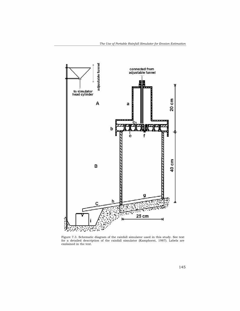
The Use of Portable Rainfall Simulator for Erosion Estimation
145
Figure 7.3. Schematic diagram of the rainfall simulator used in this study. See textfor a detailed description of the rainfall simulator (Kamphorst, 1987). Labels areexplained in the text.

Chapter 7
146
Figure 7.4. Field set-up of the rainfall simulatorin the pyroclastic flow deposits.
Figure 7.5. Graph showing the calibration of the rainfall simulator for different rainfallintensities. The level corresponds to the external pressure (exerted through theconnected funnel). The higher the level, the more pressure is applied, resulting inhigher rainfall intensities. There is a negative exponential relationship between thepressure level and rainfall intensities. The final rainfall intensity values are counter-checked with the volume of water released during the simulation time.
RAINFALL CALIBRATION AT DIFFERENT WATER LEVELS
y = 318.94x-0.97
R2 = 0.9901
0
2
4
6
8
10
12
14
16
18
20
0 20 40 60 80 100 120 140 160 180Time needed to empty 375ml of water in the cylinder (sec)
RAI
NFA
LL IN
TEN
SITY
(mm
/min
)
LEVEL <40 LEVEL -40 LEVEL -30 LEVEL -20 LEVEL -10LEVEL 0 LEVEL10 LEVEL 20 LEVEL30 Power (LEVEL 0)
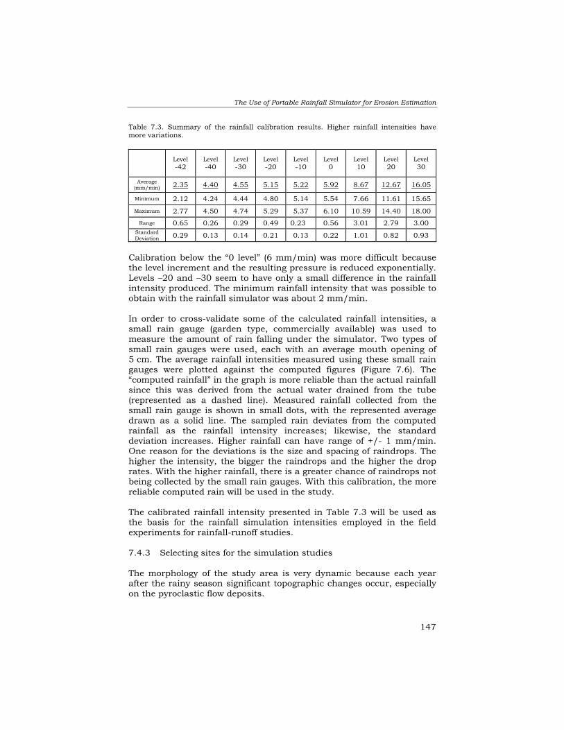
The Use of Portable Rainfall Simulator for Erosion Estimation
147
Table 7.3. Summary of the rainfall calibration results. Higher rainfall intensities have more variations.
Level -42
Level -40
Level -30
Level -20
Level -10
Level 0
Level 10
Level 20
Level 30
Average (mm/min) 2.35 4.40 4.55 5.15 5.22 5.92 8.67 12.67 16.05
Minimum 2.12 4.24 4.44 4.80 5.14 5.54 7.66 11.61 15.65
Maximum 2.77 4.50 4.74 5.29 5.37 6.10 10.59 14.40 18.00
Range 0.65 0.26 0.29 0.49 0.23 0.56 3.01 2.79 3.00 Standard Deviation 0.29 0.13 0.14 0.21 0.13 0.22 1.01 0.82 0.93
Calibration below the “0 level” (6 mm/min) was more difficult because the level increment and the resulting pressure is reduced exponentially. Levels –20 and –30 seem to have only a small difference in the rainfall intensity produced. The minimum rainfall intensity that was possible to obtain with the rainfall simulator was about 2 mm/min. In order to cross-validate some of the calculated rainfall intensities, a small rain gauge (garden type, commercially available) was used to measure the amount of rain falling under the simulator. Two types of small rain gauges were used, each with an average mouth opening of 5 cm. The average rainfall intensities measured using these small rain gauges were plotted against the computed figures (Figure 7.6). The “computed rainfall” in the graph is more reliable than the actual rainfall since this was derived from the actual water drained from the tube (represented as a dashed line). Measured rainfall collected from the small rain gauge is shown in small dots, with the represented average drawn as a solid line. The sampled rain deviates from the computed rainfall as the rainfall intensity increases; likewise, the standard deviation increases. Higher rainfall can have range of +/- 1 mm/min. One reason for the deviations is the size and spacing of raindrops. The higher the intensity, the bigger the raindrops and the higher the drop rates. With the higher rainfall, there is a greater chance of raindrops not being collected by the small rain gauges. With this calibration, the more reliable computed rain will be used in the study. The calibrated rainfall intensity presented in Table 7.3 will be used as the basis for the rainfall simulation intensities employed in the field experiments for rainfall-runoff studies. 7.4.3 Selecting sites for the simulation studies The morphology of the study area is very dynamic because each year after the rainy season significant topographic changes occur, especially on the pyroclastic flow deposits.

Chapter 7
148
The geomorphic evolution due to erosion of the 1991 pyroclastic flow deposits produced a complex topography with a wide range of gradients and forms, and a high-density network of gullies. Therefore, rainfall simulations were carried out on different deposits and at various slope angles. A total of nine deposits in four locations were sampled (Figure 7.7). For pyroclastic flow materials, sites were selected of different ages and at different distances from the crater. Plots with gradients of 20, 40, 60, 80 and 100% were selected on the 1991 pyroclastic flow materials. On the lahar and ashfall deposits, rainfall simulations were carried out on only two slopes, i.e., 20 and 40%, because of the relatively low gradients on which these sediments are deposited. Lahars were further sampled depending on their rheology, i.e., debris flows and hyperconcentrated flows. Original in situ ashfall deposits were difficult to find because they had been mostly eroded during the various rainy seasons, especially in 1991 and 1992. There was at least one site where ashfall could still be found: on a vegetated hill near the Sacobia River located in Mactan sampling area. However, the ashfall appeared to be highly compacted as compared with the initial in situ deposits. Figure 7.7 shows the areas where simulations were conducted. Most of the rainfall simulations were conducted in the last part of 1997 and the early part of 1998. During this time, most of the undisturbed pyroclastic flows were only
RAINFALL CALIBRATION USING COMPUTED AND MEASURED RAIN (mm/min)
y = 0.7777x + 0.4477R2 = 0.9004
0
1
2
3
4
5
6
7
8
9
10
0 1 2 3 4 5 6 7 8 9 10
MEASURED RAINFALL
CO
MPU
TED
RAI
NFA
LL
Figure 7.6. Plot of rainfall values measured using small rain gauges against thecomputed rain (dashed diagonal line). High rainfall intensities tend to have morevariations in the measured rainfall. Solid line is the optimal regression line for computedand measured.

The Use of Portable Rainfall Simulator for Erosion Estimation
149
found in the upper watershed, forming high terraces with deep gullies. Primary and secondary pyroclastic flows were also preserved at the distal deposit in Sacobia (Mactan).
7.5 Infiltration rates 7.5.1 Infiltration rates of the different types of deposits Infiltration rates of different deposits were studied by producing artificial rain using the rainfall simulator. A known rainfall intensity was produced over a plot of 25 x 25 cm. Infiltration rate is expressed in mm/min which was calculated from a volume of water that is infiltrated on a 25 cm² plot per unit time. High-intensity rainfall (6-12 mm/min) was applied for a duration of 15 minutes and a lower intensity (2-5 mm/min) was applied for about one hour. Runoff was measured and the volume deducted from the total rainfall magnitude. Thus, infiltration is equal to rainfall magnitude minus the measured runoff (water only). Table 7.4 shows the results of the infiltration measured on different deposits, with rainfall intensities of 2, 4, 5, 6 and 12 mm/min and on slopes of 20 and 40%. More extensive simulations were conducted on the 1991 pyroclastic flow deposits, where measurements were carried out using slopes of 20, 40, 60, 80 and 100%. Table 7.4 and Figure 7.8 present the infiltration rates of different deposits. The figure is a stacked bar of 15-minute simulations with intervals of 3, 6, 10 and 15 minutes. It can be noted that ashfall, old
Figure 7.7. Sites (shown in white dots) where rainfall simulations were conducted.

Chapter 7
150
pyroclastic flow deposits and lahars have lower infiltration capacities, due mainly to the presence of finer particles.
TOTAL AMOUNT OF
INFILTRATION (mm) IN MINUTES AFTER: SOIL TYPE
CODES For each sample
INTEN- SITY
mm/min
SLOPE %
3 min 6 min 10 min 15 min 1991 SACOBIA PF 2(A1)40 2 40 6 11 18 26 1991 SACOBIA PF 4(A1)20 4 20 11 20 28 40 1991 SA1OBIA PF 4(A1)40 4 40 11 20 32 45 1991 SACOBIA PF 5(A1)20 5 20 15 31 50 72 1991 SACOBIA PF 5(A1)40 5 40 12 21 33 47 1991 SACOBIA PF 6(A1)20 6 20 14 28 50 73 1991 SACOBIA PF 6(A1)40 6 40 4 16 34 55 1991 SACOBIA PF 12(A1)20 12 20 14 50 86 141 1991 SACOBIA PF 12(A1)40 12 40 17 50 87 146 OLD PF 6(A2)20 6 20 4 20 41 51 SANDY PF 6(A3)40 6 40 16 30 52 78 1991 UPPER PF 6(A4)20 6 20 17 31 51 79 1991 UPPER PF 6(A4)40 6 40 18 35 57 84 1991 UPPER PF 12(A4)20 12 20 28 55 99 151 PF WITH RILLS 6(A5)40 6 40 15 29 49 74 PF WITH RILLS 12(A5)40 12 40 15 49 89 148 1991 ASHFALL 6(C)20 6 20 7 18 40 57 1991 ASHFALL 6(C)40 6 40 9 26 43 64 1991 ASHFALL 12(C)20 12 20 14 46 84 134 1991 ASHFALL 12(C)40 12 40 12 44 84 133 DEBRIS FLOWS 6(B1)20 6 20 15 30 48 75 DEBRIS FLOWS 6(B1)40 6 40 15 32 54 90 DEBRIS FLOWS 12(B1)20 12 20 22 54 95 145 DEBRIS FLOWS 12(B1)40 12 40 19 48 99 155 LAHAR 6(B2)20 6 20 10 24 32 62 LAHAR WITH RILLS 6(B2)40 6 40 4 19 39 63 LAHAR 12(B2)20 12 20 18 44 87 134 LAHAR WITH RILLS 12(B2)40 12 40 18 51 90 143
Table 7.4. Total amount of infiltration at different time steps for the different types ofMt. Pinatubo deposits. The sample codes represent the parameters used in thesimulation. The values in front of the parenthesis represent the rainfall intensityused, the alphanumeric codes inside the parentheses refer to the soil code, and thevalues after the parenthesis relate to the slope of the plot in which the simulationwas conducted.

The Use of Portable Rainfall Simulator for Erosion Estimation
151
Figure 7.9 shows cumulative graphs depicting the trends in infiltration for the 15-minute simulation periods. The infiltration shows a linear trend through time for most of the deposits. The linear trend of the cumulative infiltration graph means that the effect of sorptivity on the infiltration rate is nearly zero. This can be demonstrated by the models currently used for the cumulative infiltration, such as the Philips equation (Kulitek and Nielsen, 1994).
atStI += ½
where: I = is cumulative infiltration S = sorptivity a = 2/3 Ks (saturated conductivity)
t = time Since I is linearly related to t, S must be zero. The non-effect of the sorptivity is explained by the high initial moisture content of the soil and the high intensities used in the simulation. This implies that the amount of infiltration in the deposit is continuously in a steady condition. Although the runoff generally starts after one minute of rainfall, infiltration proceeds linearly through time, at least during the 15-minute simulation. The increase in infiltration is about twofold between 6 and 12 mm/min rainfall intensity. From Table 7.4 it can be concluded that strong rainfall intensity is the main factor in the increase in infiltration. On the other hand, the difference in slope
Figure 7.8. Stacked bar chart of the infiltration results for the different deposits. Referto Table 7.4 for the identification of codes.
INFILTRATION AT 4 TIME INTERVALS OF DIFFERENT MT. PINATUBO DEPOSITS
020406080
100120140160180
2(A1
)40
4(A1
)20
4(A1
)40
5(A1
)20
5(A1
)40
6(A1
)20
6(A1
)40
6(A2
)20
6(A3
)40
6(A4
)20
6(A4
)40
6(A5
)40
6(C
)20
6(C
)40
6(B1
)20
6(B1
)40
6(B2
)20
6(B2
)40
12(A
1)20
12(A
1)40
12(A
4)20
12(A
5)40
12(C
)20
12(C
)40
12(B
1)20
12(B
1)40
12(B
2)20
12(B
2)40
Type of deposit
INFI
LTR
ATIO
N (m
m)
3min 6min 10min 15min

Chapter 7
152
has little influence on the infiltration. This also indicates the low initial water content of the soil. When there is much water in the soil, the water may runoff surficially especially on steep slopes. 7.5.2 Infiltration rates of the 1991 pyroclastic flow deposits More extensive infiltration tests were conducted on the 1991 pyroclastic flow deposits. Figure 7.10 shows the cumulative infiltration of pyroclastic flows with rainfall intensities of 2, 4, 5, 6 and 12 mm/min. Simulations with lower intensities were extended to an hour to observe the runoff. The graphs are coded. The numbers before the parenthesis indicate the rainfall intensity that was applied, and the values on the right side indicate the slope angle of the plot where the simulation was conducted. From Figure 7.10 it can be concluded that, even during a longer simulation period, infiltration behaves in a linear trend. It also shows that the higher the rainfall intensity, the higher the infiltration rate. 7.5.3 Infiltration relationships on the different deposits In order to understand the factors influencing runoff, several parameters were measured and analyzed using linear regression (see Table 7.5). That table shows the R2 correlation coefficient; P-value, a measure of significance; and the coefficient that depicts the rate of change in the variable. The P-values should have a value of 0.05 or less at 95% confidence level. However, for comparative studies on the effects of different parameters through time intervals, comparing R2 and the coefficient gives an idea of the relationships of the parameters, given a certain simulation time.

The Use of Portable Rainfall Simulator for Erosion Estimation
153
Figure 7.10. Cumulative infiltration curve of the dominant type of 1991 pyroclastic flowdeposits, derived from rainfall simulations with intensities of 2, 4, 5, 6 and 12 mm/min and onmicro-plots with slopes of 20, 40, 60, 80 and 100%. Simulation times at lower intensities wereextended to one hour.
0
50
100
150
200
250
0 10 20 30 40 50 60RAINFALL DURATION (min)
INFI
LTR
ATIO
N (m
m)
2(40) 2(60) 2(100) 4(20) 4(40) 4(60) 4(80) 4(100) 5(20)5(40) 5(60) 5(80) 5(100) 6(20) 6(40) 6(60) 6(80) 6(100)12(20) 12(40) 12(60) 12(80) 12(100)
12mm
2mm
4mm
6mm
Figure 7.9. Cumulative infiltration curves of different Mt. Pinatubo deposits, derived from rainfallsimulations using rainfall intensities of 2, 4, 5, 6 and 12 mm/min on micro-plots with slopes of 20and 40%. This data set is also shown in Table 7.4.
0
20
40
60
80
100
120
140
160
0 2 4 6 8 10 12 14 16RAINFALL DURATION (min)
INFI
LTR
ATIO
N(m
m)
2(A1)40 4(A1)20 4(A1)40 5(A1)20 5(A1)40 6(A1)20 6(A1)40 12(A1)2012(A1)40 6(A2)20 6(A3)40 6(A4)20 6(A4)40 12(A4)20 6(A5)40 12(A5)406(C)20 6(C)40 12(C)20 12(C)40 6(B1)20 6(B1)40 12(B1)20 12(B1)406(B2)20 6(B2)40 12(B2)20 12(B2)40
12mm
6mm
2-4mm
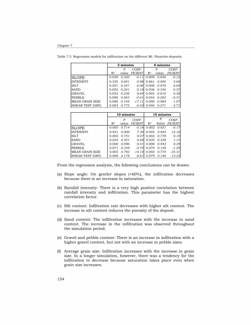
Chapter 7
154
Table 7.5. Regression models for infiltration on the different Mt. Pinatubo deposits.
3 minutes 6 minutes
R2 P
value COEF-
FICIENT R2 P value
COEF- FICIENT
SLOPE 0.038 0.320 -0.11 0.009 0.640 -0.12 INTENSITY 0.335 0.001 0.98 0.861 0.000 3.69 SILT 0.051 0.247 -0.06 0.000 0.978 0.00 SAND 0.053 0.241 0.19 0.036 0.336 0.37 GRAVEL 0.053 0.238 0.64 0.002 0.818 0.30 PEBBLE 0.000 0.943 -0.01 0.044 0.282 -0.31 MEAN GRAIN SIZE 0.080 0.144 17.11 0.000 0.969 1.07 SHEAR TEST (DRY) 0.003 0.772 -0.42 0.046 0.271 -3.71
10 minutes 15 minutes
R2 P
value COEF-
FICIENT R2
P value
COEF- FICIENT
SLOPE 0.005 0.714 -0.18 0.002 0.831 -0.17 INTENSITY 0.931 0.000 7.34 0.945 0.945 12.16 SILT 0.004 0.751 0.07 0.003 0.778 0.10 SAND 0.033 0.351 0.68 0.035 0.338 1.15 GRAVEL 0.000 0.996 0.01 0.000 0.942 0.29 PEBBLE 0.071 0.169 -0.75 0.079 0.148 -1.29 MEAN GRAIN SIZE 0.003 0.792 -14.14 0.003 0.774 -25.31 SHEAR TEST (DRY) 0.069 0.178 -8.61 0.079 0.146 -15.25
From the regression analysis, the following conclusions can be drawn: (a) Slope angle: On gentler slopes (<60%), the infiltration decreases
because there is an increase in saturation. (b) Rainfall intensity: There is a very high positive correlation between
rainfall intensity and infiltration. This parameter has the highest correlation factor.
(c) Silt content: Infiltration rate decreases with higher silt content. The
increase in silt content reduces the porosity of the deposit. (d) Sand content: The infiltration increases with the increase in sand
content. The increase in the infiltration was observed throughout the simulation period.
(e) Gravel and pebble content: There is an increase in infiltration with a
higher gravel content, but not with an increase in pebble sizes. (f) Average grain size: Infiltration increases with the increase in grain
size. In a longer simulation, however, there was a tendency for the infiltration to decrease because saturation takes place even when grain size increases.

The Use of Portable Rainfall Simulator for Erosion Estimation
155
(g) Shear strength: Infiltration decreases with the increase in shear strength of the material. More compacted sediments increase in shear strength and this reduces porosity, leading to less infiltration.
7.6 Runoff measurements 7.6.1 Runoff results on different types of Mt. Pinatubo deposits To determine the runoff response of the various deposits, in situ rainfall simulations were conducted on eight types of deposits. Rainfall intensities of 2, 4, 5, 6 and 12 mm/min were used. The results of the simulations are shown in Table 7.6. Runoff is highly influenced by rainfall intensities. When there is a constant infiltration rate, infiltration increases with rain intensity. Simulation tests using an intensity of 6 mm/min resulted in high runoff on ashfall, debris flows and old pyroclastic flows. These deposits contain more fine particles. On the other hand, results using the 12 mm/min simulation show that ashfall, debris flows and the new pyroclastic flows have the highest runoff values. Clearly, high rainfall intensities yield higher runoff. It is noticeable that on steep slopes (80 and 100%) runoff is lower than on gentler slopes (20 and 40%). This is due to the micro-depressions that are formed or have developed on steeper slopes. Steep slopes naturally form micro-depressions or micro-staircase structures, which retard the flow in the small depressions. This was maintained throughout the simulation. It appears that on slopes of 20 and 40%, water saturation and runoff increase. 7.6.2 Runoff simulation on the hot pyroclastic flows The 1991 pyroclastic flows were deposited under high temperatures. Although they remained hot even for several years, it was impossible to find hot deposits on the surface when this field campaign was conducted in 1997. It is highly feasible that hot pyroclastic flows still exist at certain depths where the overburden is still thick. To simulate the runoff on hot pyroclastic flows, the rainfall simulation experiment could only be performed in the laboratory.

Chapter 7
156
Table 7.6. Results of runoff (ml/min) with respect to different rainfall intensity and slopes. Intervals of four periods are shown in order to delineate the different rate of runoff. Average runoff is shown in the last column, which represents the 15-minute simulation.
SITE TYPE OF DEPOSIT
INTEN-SITY
SLO-PE
0-3 min
3-6 min
6-10 min
10-15 min
AVE-RAGE
2 40 0 12 21 30 16 4 20 20 68 114 100 76 4 40 30 46 68 86 58 5 20 0 1 24 44 17
PRIMARY PYROCLASTIC
FLOW DEPOSITS 5 40 80 120 138 144 120 6 20 89 173 164 228 164 6 40 324 457 432 459 418
12 20 502 489 564 506 515 MA
CTA
N A
RE
A
SECONDARY PYROCLASTIC
FLOW DEPOSITS 12 40 475 556 618 509 539 6 20 320 328 331 547 381 PASIG PRE-1991 PF
DEPOSIT 6 40 41 111 133 164 112 6 20 14 106 165 160 111 6 40 0 20 58 71 37
12 20 180 413 391 457 360 MT.
D
OR
ST PRIMARY
PYROCLASTIC FLOW DEPOSITS
12 40 265 372 384 361 346 6 20 223 169 37 166 149 6 40 199 22 116 105 110
12 20 490 84 163 125 215 ASHFALL
12 40 519 79 132 134 216 6 40 71 150 185 215 155
12 40 461 522 504 408 474 6 40 318 372 351 352 348
12 40 431 454 483 475 461 6 20 64 114 161 182 130
MA
CTA
N
HYPERCONCEN-TRATED LAHAR
DEPOSIT
12 20 52 68 89 70 6 20 339 406 416 467 407 6 40 398 573 443 449 466
12 20 173 267 445 357 310 MANCA-TIAN
DEBRIS FLOW DEPOSIT
12 40 430 639 534 592 549 To simulate the effect of high temperatures, a pan 26 x 34 x 17 cm was filled with the 1991 pyroclastic flow materials and placed inside an oven. The sample was heated for almost six hours. The pan was removed and placed under the rainfall simulator as fast as possible so that little heat was lost. The pan was mounted to have a slope of 20%. A thermometer was inserted in the base of the sample to measure the rate of heat loss. The rainfall simulation was then carried out with different intensities, and the runoff was collected and measured at given time intervals. Temperatures reached as high as 359°C, but when the sample was placed under the rainfall simulator, the temperature dropped quickly due to the effect of the ambient room temperature.
The Use of Portable Rainfall Simulator for Erosion Estimation
157
Figure 7.11 shows the temperature drop rate of different initial temperatures and different rainfall intensities. It demonstrates the relation between rainfall and the cooling rate of the hot pyroclastic flows. The graph shows a common trend, when the temperature starts to decrease uniformly slowl at a certain time in the simulation. The threshold temperature is slightly higher than 100°C, the boiling point of water. Lower rainfall intensities (3 mm/min) start to stabilize the temperature after a 20-minute simulation, a bit later compared with higher rainfall intensity simulations. It also appears that the cooling around 100°C of hot pyroclastic flow is nearly synchronous with the start of runoff. Figure 7.12 shows the runoff collected during the simulations. The start of runoff was generally observed after nine minutes of simulation, but a longer time was required for low rainfall intensities. 7.7 Erosion rates Erosion rate is defined as the amount of soil loss in a specified time period over an area of land (here at micro-plot level). It is expressed in units of mass per unit area, such as tons per hectare or kilograms per square meter, which is a suitable unit for plot level. In this case, our micro-plot uses g/625 cm2 or each unit is equivalent to 16 g/m2. On the other hand, sediment yield refers to a mass of sediment that crosses a boundary, such as the edge of a field or the outlet of a watershed, and is expressed in units of total mass (kg), mass per unit width of boundary (kg/m), or mass per unit area (kg/m2) (Nearing et al., 1994). In this study, sediment yield is expressed in total mass (grams) which is limited to the plot size of 625 cm2. The description of erosion refers to the sediments entrained during simulation, including splash detachment. The effect of splash detachment was not measured independently since it makes little contribution to the overall erosion. They are expressed in weight (grams) measured after drying. The rate of erosion is influenced by many factors, including the concentration of runoff, rainfall intensities and plot slopes.

Chapter 7
158
Figure 7.11. Cooling rate of hot pyroclastic flow sediments (experiments conducted in thelaboratory using a rainfall simulator and oven-heated pyroclastic flow sediments). Theexperiments were conducted using different rainfall intensities and temperatures ofsediments.
0
50
100
150
200
250
1 8 15 22 29 36 43 50 57 64 71TIME (min)
INIT
IAL
TEM
PER
ATU
RE
OF
P.F.
(°C
)
7mm 8mm 6mm 4mm 3mm
Figure 7.12. Runoff measured during the laboratory simulation of hot pyroclastic flowsediments.
0
100
200
300
400
500
600
0 5 10 15 20 25 30TIME (min)
RU
NO
FF V
OLU
ME
(ml)
3mm-120°C 6mm-164°C 6mm-202°C 4mm-131°C

The Use of Portable Rainfall Simulator for Erosion Estimation
159
7.7.1 Erosion rates for different types of deposits To compare the erosion rates of different deposits, tests were carried out with rainfall intensities of 6 and 12 mm/min and slopes of 20 and 40%. Table 7.7 gives the results of the erosion measurements using different intensities and slopes.
During low rainfall intensities, i.e., 2, 4 and 5 mm/min, no erosion was measured except for ashfall deposits. With higher rainfall intensities, lahars such as debris flows and hyperconcentrated flow deposits
SOIL LOSS
SITE TYPE OF DEPOSIT
INTEN-SITY SLO-PE 0-3
min 3-6 min
6-10 min
10-15 min
AVERAGE
2 40 0 0 0 0 0
4 20 1 1 1 1 1
4 40 1 1 0 0 1
5 20 0 0 0 0 0
PRIMARY PYROCLASTIC
FLOW DEPOSITS
5 40 3 1 0 1 1
6 20 14 6 4 9 8
6 40 57 52 18 13 35
12 20 102 26 21 12 40
MA
CTA
N
SECONDARY PYROCLASTIC
FLOW DEPOSITS
12 40 145 119 76 51 98
6 20 5 9 15 6 9
12 40 39 45 41 59 46
12 20 64 38 29 24 39
6 40 6 11 7 7 8
MT.
DO
RS
T
PRIMARY PYROCLASTIC
FLOW DEPOSITS
12 40 59 39 17 8 31
6 20 19 19 15 11 16
6 40 19 11 9 8 12
12 20 63 26 21 17 32 ASHFALL
12 40 40 18 13 7 19
6 40 49 17 15 7 22
12 20 98 53 17 15 46
12 40 101 28 17 5 38
MA
CTA
N
HYPERCON-CENTRATED
LAHAR DEPOSIT
6 20 21 26 15 8 18
6 20 3 18 26 15 16
6 40 10 12 5 0 7
12 20 102 43 29 23 49
MA
NC
ATI
AN
DEBRIS FLOW
DEPOSIT 12 40 117 67 97 89 93
Table 7.7. Soil loss (in grams) results from the simulations conducted with rainfallintensities of 2, 4, 5, 6, and 12 mm/min and plot slopes of 20 and 40%.
Chapter 7
160
produced high erosion. Pyroclastic flows (A1) yielded the highest erosion, especially at a 40% slope. Extensive simulations were also done on the 1991 pyroclastic flows. For intensities of 6 mm/min, the pyroclastic flow deposits yielded high sediment rates. For the 12 mm/min rainfall, some types of soil produced high sediments. In some cases an abrupt increase in erosion occurred, which may suggest some collapse of the materials on the slope. 7.7.2 Regression analysis on erosion From Table 7.8, the following conclusions can be drawn regarding the relationships of erosion rates with the individual factors: (a) Slope angle: As could be expected, erosion increases with increasing
slopes. The relationship improves with longer-duration rainfall. (b) Rainfall intensity: Higher rainfall intensity yields higher erosion.
This factor is highly significant in the erosion process. As the rainfall simulation increases in time, the effects of slope on the erosion have little influence in this situation.
(c) Silt content: With increasing silt content comes a decrease in
erosion. The relationship is reasonably similar for different simulation times. Fine sediments act as a cementing agent that enhances cohesion of the deposit, leading to less erosion.
(d) Sand, gravel and pebble content: Erosion is higher with increasing
sand content. The effect of the relationship does not improve with time. Sands are easily detachable and subject to collapse when saturated, and they can easily be entrained. Increase in gravel content results in increase in erosion. The relationship does not improve with simulation time. Gravel is often associated with high percentages of sand, and the results indicate the effect of the sand-size particles.
(e) Mean grain size: There is an increase in erosion with increasing
average grain size. The overall mean grain size is within the sand fraction.
(f) Shear strength: Erosion increases with decreasing shear strength. 7.7.3 Erosion results for the 1991 pyroclastic flow deposits Similar extensive simulations were carried out on the 1991 pyroclastic flow deposits. The results of these experiments disclosed that at low

The Use of Portable Rainfall Simulator for Erosion Estimation
161
intensities there is little or no erosion. The slope of 40% gives the highest erosion, both at 6 and 12 mm/min-rainfall intensity. There is no clear relation between slope and amount of erosion. Simple and multiple regression statistics were also conducted in order to see the influence of different factors on the erosion rate for the pyroclastic flow deposits. Table 7.9 shows the results of the regression for each parameter. Table 7.8. Linear regression model results used to determine the effects of different parameters in the behaviour of erosion. Regression models were calculated for four time intervals.
3 minutes 6 minutes
R2 P
value COEF-
FICIENT R2 P
value COEF-
FICIENT SLOPE 0.003 0.775 0.76 0.013 0.580 3.11 INTENSITY 0.722 0.000 32.64 0.576 0.000 62.05 SILT 0.007 0.675 -0.48 0.013 0.578 -1.35 SAND 0.008 0.669 1.68 0.005 0.731 2.87 GRAVEL 0.024 0.449 9.59 0.027 0.425 21.49 PEBBLE 0.034 0.369 -2.64 0.014 0.567 -3.61 MEAN GRAIN 0.001 0.898 35.88 0.006 0.701 229.69 SHEAR TEST (DRY) 0.069 0.195 -44.05 0.036 0.354 -67.64
10 minutes 15 minutes
R2 P
value COEF-
FICIENT R2 P
value COEF-
FICIENT SLOPE 0.018 0.511 6.38 0.023 0.465 11.22 INTENSITY 0.483 0.000 97.99 0.373 0.001 136.30 SILT 0.012 0.588 -2.26 0.012 0.595 -3.51 SAND 0.003 0.791 3.82 0.005 0.744 7.45 GRAVEL 0.027 0.419 37.57 0.024 0.447 56.06 PEBBLE 0.022 0.468 -7.87 0.020 0.495 -11.73 MEAN GRAIN 0.014 0.567 588.37 0.020 0.486 1132.25 SHEAR TEST (DRY) 0.042 0.316 -126.0 0.033 0.374 -177.24
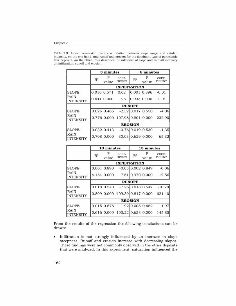
Chapter 7
162
Table 7.9: Linear regression results of relation between slope angle and rainfall intensity, on the one hand, and runoff and erosion for the dominant type of pyroclastic flow deposits, on the other. This describes the influence of slope and rainfall intensity on infiltration, runoff and erosion.
3 minutes 6 minutes
R2 P value
COEF- FICIENT R2 P
value COEF-
FICIENT
INFILTRATION SLOPE 0.016 0.571 0.02 0.001 0.896 -0.01 RAIN INTENSITY 0.641 0.000 1.26 0.933 0.000 4.15
RUNOFF SLOPE 0.026 0.466 -2.32 0.017 0.550 -4.06 RAIN INTENSITY 0.776 0.000 107.98 0.801 0.000 232.90
EROSION SLOPE 0.032 0.413 -0.76 0.019 0.530 -1.35 RAIN INTENSITY 0.708 0.000 30.03 0.629 0.000 65.32
10 minutes 15 minutes
R2 P value
COEF- FICIENT R2 P
value COEF-
FICIENT
INFILTRATION SLOPE 0.001 0.890 -0.03 0.002 0.849 -0.06 RAIN INTENSITY 4.154 0.000 7.61 0.970 0.000 12.56
RUNOFF SLOPE 0.018 0.540 -7.26 0.018 0.547 -10.79 RAIN INTENSITY 0.809 0.000 409.39 0.817 0.000 621.40
EROSION SLOPE 0.015 0.576 -1.92 0.008 0.682 -1.97 RAIN INTENSITY 0.616 0.000 103.22 0.628 0.000 145.85
From the results of the regression the following conclusions can be drawn:
• Infiltration is not strongly influenced by an increase in slope
steepness. Runoff and erosion increase with decreasing slopes. These findings were not commonly observed in the other deposits that were analyzed. In this experiment, saturation influenced the

The Use of Portable Rainfall Simulator for Erosion Estimation
163
erosion process since gentler slopes can be easily saturated. Likewise, less rain is experienced on steeper slopes.
• Infiltration, runoff and erosion increase with increasing rainfall
intensity. The relationships are observed at the same level of confidence with different time steps.
7.8 Comparison with rainfall simulation results from literature Kamphorst (1987) made several rainfall simulations, using the same type of rainfall simulator, in the province of Limburg, located in the southern part of the Netherlands. The topography is rolling and consists mostly of loess soils. Table 7.10 shows a comparison between Kamphorst's experiments and this work. Table 7.10. Comparison of rainfall simulation results for deposits from Mt. Pinatubo with those from Limburg (Kamphorst, 1987)
Runoff Volume
(ml)
Soil loss (dry
weight) (g)
Sediment concentrati
on (g/ml)
THIS WORK Pyroclastic flow deposit (Mactan) 268 41 162 Pyroclastic flow deposit (Mt.Dorst)
41 14 414
Ashfall deposit 668 57 86 Hyperconcentrated flow deposit(Mactan)
954 146 163
Pyroclastic flow deposit (Mactan) 214 18 86 Debris flow (Mancatian) 191 10 51 Hyperconcentrated flow deposit(Pasig)
519 64 130
KAMPHORST WORK Aeolian sand 641 17 27 Aeolian loamy sand 806 35 43 Aeolian sandy loam 864 40 46 Coarse loess 822 39 48 Medium loess 677 18 27 Fine loess 457 8 18 Riverine sandy loam 322 5 16 Riverine clay loam 692 5 7 Riverine clay 465 4 9
Soils from Limburg produce higher runoff than the Pinatubo deposits. On some erodible Limburg materials, e.g., aeolian sands and coarse

Chapter 7
164
loess, comparable amounts of soil loss can be measured. However, sediment concentrations for the Pinatubo deposits are significantly higher. This would lead to the conclusion that Pinatubo deposits are far more erodible than Limburg soils despite high Pinatubo’s infiltration rates. 7.9 Conclusions Field experiments were conducted to study the hydraulic properties of the different volcanic deposits. Extensive plot-scale rainfall simulations using a portable rainfall simulator were carried out in order to study the infiltration and runoff for different rainfall intensities, slopes angles, grain sizes and soil strengths. The following conclusions were derived: • The main sources of lahars are the pyroclastic flow materials
deposited in 1991. Grain size distribution of this type of deposit shows that about 60 to 80% of the sediments consist of medium to fine sands. These materials were deposited hot and were prone to secondary explosions, which may generate secondary pyroclastic flows. Grain size analysis of primary and secondary pyroclastic flow deposits revealed great similarity with only slightly less finer fractions in the latter due to elutriations produced during the redeposition. The median grain size of active lahars and lahar deposits is in the range of 0.5 to 2 mm, which is coarser as compared to pyroclastic flows since the finer fractions are washed away by water during the transport.
• Pyroclastic flows, lahars and other sand-rich deposits at Mt.
Pinatubo exhibit low shear strength and cohesion. Results from the measurements of shear strength in the field show a significant decrease in shear strength between dry and wet deposits. The deposits instantaneously loose strength when saturated.
• Studies on infiltration and runoff were done using a rainfall
simulator. The advantage of the simulator is that it can test infiltration and runoff at natural soil conditions. The original design of the simulator is to give a shower of 3 minutes with rainfall intensity of 6mm/minute on a test plot with a slope steepness of 20%. The rainfall simulator was modified in order to quantify the effects of other slope angles and rainfall intensities on the infiltration and runoff. After modification and calibration, the instrument could be operated to give showers from 2 up to 12 mm/minute on slopes ranging from 0% to 100%.

The Use of Portable Rainfall Simulator for Erosion Estimation
165
• The infiltration rates of most of the deposits are very high. For rainfall intensities of 2 to 6 mm/min, infiltration generally decreases in a linear way. For high rainfall intensities, the infiltration is also very high and the difference is large compared with the lower intensities. However, the relation is less clear for larger simulation times of 10 to 15 minutes, due to the effect of soil collapse.
• The high infiltration capacity of Mt. Pinatubo pyroclastic
deposits is due to the high porosity of the sediments that resulted from poor sorting due to rapid deposition. The bulk of the deposit consists of medium to coarse angular sand.
• Occurrences of very high intensity and short-duration rainfall
are very likely at Mt. Pinatubo, and some short-duration rainfall events may exceed 12 mm/min. These are still within the rainfall intensities used in the rainfall simulations. However, rainfall with less than 1 mm/min sustained for 30 minutes is enough to trigger lahars. There is a sharp increase in sediment production as simulation time is increased especially with high intensity rainfall.
• The infiltration data shows generally a linear trend due to the
effect of sorptivity that is nearly zero as explained by the high initial moisture content and the high intensities used in the simulation. The slope of the trend is gradual, although constant, and it indicates that infiltration remains generally steady even if runoff starts.
• Regression analysis on the infiltration and the effects of
different parameters, i.e., slope, rainfall intensity, grain size and soil strength, indicated that rainfall intensity has the greatest influence on the infiltration. An increase in fine sediments and slopes less than 60% decrease infiltration because there is a greater tendency of water saturation.
• Runoff results show a general decrease with increasing slope
angle. At slopes of 40 to 60%, the runoff is greater than on steeper slopes, i.e., 80 and 100%. Similar observations were also made by other researchers, such as Mannaerts (1992). A possible explanation is that on steep slopes micro-depressions or “staircase” features are formed in the soil, which retard the effect of runoff.
• Erosion results from the experiments show that rainfall
intensities below 6 mm/min do not entrain a significant volume of sediments. Higher rainfall intensities from 6 to 12 mm/min
Chapter 7
166
result in a drastic increase in soil runoff. Regression analysis on the behaviour of sediment yield with several parameters revealed that the increase in rainfall intensity and slope conditions lead to higher erosion. Erosion is high on soils with a higher sand content.
• Experiments conducted in the laboratory regarding the cooling
rate and runoff of hot pyroclastic flows revealed that runoff starts after a steep decline in the cooling rate of the hot pyroclastic flows. The initial cooling rate of hot pyroclastic flows drops exponentially until it reaches a temperature slightly above 100ºC, which is maintained for some time, while runoff starts.
• There are some drawbacks in the use of a small plot (25 cm by
25 cm) for conducting infiltration and runoff studies. One major drawback is that the effect of long slopes is not fully accounted for. Slope configuration such as the presence of rills and gullies are not well represented. It is noticeable in the simulations that rainfall intensities below 6 mm/min do not lead to significant erosion, while on a catchment scale, much smaller rainfall intensities could already lead to significant lahars. It was established in the experiments that highly saturated sediments could lead to accelerated sediment erosion. One observable reason is that saturation occurs more on longer slopes due to the effect of overland flow and its contribution to the formation of rills and gullies, which may contribute to soil collapse. These catchment scale effects cannot be quantified using plot scale experiments.
• The erosion figures are only indicative of relative erodibility and
the measured values cannot be treated as absolute values when extrapolating them to catchment-scale erosion studies.

Cell-based Dynamic Modeling of Lahar Initiation in Pyroclastic Flow Deposits
167
Chapter 8: Cell-based Dynamic Modelling of Lahar Initiation in Pyroclastic Flow Deposits
8.1 Introduction Process-based models, which are abstractions of reality, are created in order to simulate and understand the relationships of natural processes under certain physical rules and conditions. There are several types of models, ranging from very simple one-dimensional (1D) models using a single equation to very complex models involving many parameters with several mathematic and physical equations simulated in a 4D (x, y, z and time) environment. Cell-based physical models for catchment studies are not simple; they involve several physical parameters and processes acting on a catchment. These models vary according to the scale at which they are used. Several surface hydrologic models have been designed to simulate rainfall and runoff, even at catchment scale. Most of these models are used for soil loss estimation at a variety of scales (Morgan et al., 1994; Kirkby and Cox, 1995; Morgan et al., 1998). Depending on the catchment’s physical conditions and the desired results, each model has its own input parameter requirements. Commonly, such hydrologic models, which simulate rainfall, infiltration, erosion and water discharge, are aimed at erosion management, irrigation, water conservation and inundation studies. Hydrologic models for simulating rainfall-runoff relations on recently erupted and sediment-rich volcanoes entail very different concepts. Few models exist and those that do are mostly at the developmental stage and are generally site-specific. Models on a volcanic environment are to some extent site-sensitive, owing to the high heterogeneity of the catchment’s inherent physical parameters, such the grain sizes of the newly deposited sediments, the temperature of emplacement, sorting, cohesion, distribution, and other properties that were never measured in case of new eruptions. Other significant differences from the current erosion models are as follows: • Different flow conditions exist in such volcanic catchments, ranging
from muddy stream flow to hyperconcentrated flow and debris flow • Generation of high sediment concentrations takes place due to the
high erodibility of sediments and bank collapse

Chapter 8
168
In this study, our main interest is to develop a cell-based catchment-scale physical model in order to simulate rainfall events in the catchment and predict the resulting lahar hydrographs, taking into account the specific local physical conditions. Several physical parameters were used to validate the model and this entailed field monitoring and measuring active lahars. 8.2 Objectives of this chapter The objectives of this chapter are the following: • To develop a runoff model that will simulate a short storm (a few
hours) on the catchment and predict the erosion of the pyroclastic flow deposits and the resulting lahar hydrographs.
• To demonstrate the effect of stream piracy in the change of lahar
magnitude of catchments. • To estimate, given a certain rainfall, the magnitude of lahars, the
volumetric concentration, duration of flow, velocity of the flow, and lahar discharge through time.
• To study the different catchments’ physical attributes that affects
the lahar model. • To analyse the sensitivity of different parameters in order to
understand the controlling factors in the lahar discharge model. 8.3 Current catchment-scale cell-based erosion models 8.3.1 Models designed for water resources management studies This section gives a brief overview of hydrologic erosion models that have been developed for use in erosion and water resources management. Depending on their specific purpose, they required a range of physical parameters or factors. Models can be lumped or semi-distributed. The following are some of the widely used models. The USLE (Universal Soil Loss Equation) considers the soil erodibility factor, crops, slope length and erosion control as input parameters. Later, MUSLE was developed replacing the rain energy factor with the runoff energy factor (Williams, 1975). The SCS (Soil Conservation Service) model is among the most widely used models in water resources planning. It was developed for agricultural purposes and also extended to suburban and urban areas. Its major input parameters include land-use and soil type (Ragan, 1980). The WEPP (Water Erosion Prediction Project) model allows continuous monitoring of erosion in any given time and space. This model is very useful when introducing remote
Cell-based Dynamic Modeling of Lahar Initiation in Pyroclastic Flow Deposits
169
sensing data as parameter input (Ballerini, et al., 1996). TOPMODEL is a physically based semi-distributed hydrologic forecasting model for predicting and subsequently understanding the rainfall-runoff mechanism. HEC-1 is a semi-distributed model and one of the most widely used hydrologic single event models developed by the US Army Corps of Engineers (USACE). It was designed to simulate the surface runoff from precipitation by representing the basin as interconnected compartments, each having its own physical parameters. A group of USACE personnel were also involved in the study of Mt. Pinatubo during the first four years. They used the HEC-1 model to predict runoff and peak discharge of some catchments at Mt. Pinatubo (USACE, 1996). These models ranged from 1-dimensional to semi-distributed that are extensively used for agricultural purposes measuring erosion and runoff. They cannot be fully adopted for the conditions of Mt. Pinatubo for simulating lahars when detailed catchment and terrain conditions are important factors. Recently, many modellers have fully adopted the use of digital terrain models (DTMs) and other thematic maps to be part of the input parameters in hydrologic models. These models can be categorized as grid-based or cell-based distributed models. The input from a DTM in such grid-based hydrologic models is becoming more demanding than that for the lumped models. The topography of the catchment has a major impact on the hydrologic processes active in the landscape (Moore et al., 1991). Speight (1974) listed about 20 topographic attributes that can be used to describe a landform and each attribute has important weights, depending on the hydrologic model. These models tend to replicate in more detail the physical conditions of the catchment. The following are some of the currently distributed models that are available. LISEM (Limburg Soil Erosion Model) is one of the first examples of a physically based model that is completely incorporated in a raster geographic information system (GIS). It incorporates several processes, such as rainfall, interception, surface storage in micro-depressions, infiltration, vertical movement of water in soil, overland flow, channel flow, detachment by rainfall and throughfall, detachment by overland flow, and transport capacity of flow (De Roo et al., 1996). Other models include ANSWERS (Aerial Non-Point Source Catchment Environment Response Simulation Model) (Beasly et al., 1980); AGNPS (Agricultural Non-point Source Pollution Model) (Young et al., 1989); and SHE (Système Hydrologique Européen), a fully distributed hydrologic model that requires the highest amount of physical parameters (Abbott and Refsgaard, 1996). Although these distributed models exist, routing of flows do not consider rheologic component of lahar flows, likewise they do not calculate the sediment concentration of the flow. The high volumetric concentration of sediment and water in the flow would greatly affect the hydrograph.

Chapter 8
170
8.3.2 Models for simulating volcanic processes In the field of volcanology, there are only a few existing models that simulate and integrate the different volcanic processes. Modelers try to do simulations of different volcanic processes in order to study the different sensitive parameters that control the mechanism. Existing models such as those for volcanic landslides and debris avalanches were developed by Di Gregorio et al., (1994), using 2D cellular automata on Ontake Volcano. The cellular automata model can be seen as a 2D plane, partitioned into square cells representing portions of the surface, with corresponding altitude and physical characteristics of the debris flow column. The advantage of this model using cellular automata is that it can serve as an alternative to differential calculus in the description of complex phenomena. The complex nature of lava flows represents generally unconfined flow of the liquid, whose phases, temperature, rheology and flux rate vary with time (Wadge et al., 1994). Barca et al., (1993), Wadge et al., (1994) and Crisi et al., (1996) used parallel computing tools in modelling the Etnean lava flows. Pyroclastic flows were also modelled by Beget and Limke (1998), using 2D kinematic and rheologic models. Levine and Kieffer (1991) used topographic data, estimates of volumetric flow rate, and a Manning coefficient appropriate for the channel to predict zones of erosion and deposition, and hazards for pyroclastic flows. Pyroclastic flows were also modelled by Beget and Limke (1998), using 2D kinematic and rheologic models. Lahars are complex flows to model. From the initial erosion to the flow process, the supply and entrainment of new sediments mixed with water can change dynamically. The highly dynamic changes of rheology from muddy stream flow to hyperconcentrated flow to debris flow and vice versa have been commonly observed in the field during the intense activity of lahar flows - thus making a lahar model quite complex. Lava flows and lahars, since they are non-Newtonian flows, differ remarkably from the many existing hydrologic models. The rheology of flows has to be treated to arrive at a more realistic approach. Calculation of mass and energy transport in viscous flows has been treated using the Navier-Stokes and Bingham equations (Ishihara et al., 1989; Wadge et al., 1994). The physics of lahars or debris flows have been extensively modelled using laboratory experiments (Takahashi, 1978, 1980; Savage, 1984, 1989, 1993; Savage and Hutter, 1989, 1991; Mizuyama and Yazawa, 1987; Chen, 1988a, b; O’Brien et al., 1993; Major and Iverson, 1999) as cited by Pierson (1998). Such methods have not been tested, parameterised, calibrated or tested in field conditions for reliable predictions, particularly of travel time (Pierson, 1998). Likewise, little work has been done on trying to integrate these models into a catchment-scale distributed model.
Cell-based Dynamic Modeling of Lahar Initiation in Pyroclastic Flow Deposits
171
Rainfall-lahar runoffs were analyzed at Mt. Pinatubo using the HEC-1 and HEC-2 models established by the US Army Corps of Engineers (USACE). A group of USACE personnel were commissioned to study the lahars in order to make technical suggestions about the engineering design of lahar engineering mitigation. Their studies cover the year 1992 to 1993, just before the October 1994 catchment capture. Their study used a semi-distributed catchment-scale model. The results of the peak flow hydrograph simulations are presented as probabilities of recurrence intervals, using time frames of 2, 5, 10, 20 and 100 years. Likewise, the Japan International Cooperating Agency (JICA), in cooperation with the local Department Public Work and Highways (DPWH), started a study in November 1993. Their study covers the Sacobia and Abacan catchments. The Storage Function Method was employed for the flood analysis because it can express the non-linearity of the rainfall-runoff relation and it has been used widely for a long time to generate hydrographs. The method involves constructing a basin runoff for each river, based on the sub-basin division and topographic conditions. The long-term design condition is established on the assumption that the field of 1991 pyroclastic flow deposits will have hardened and the sediment delivery rate will be equivalent to that in the pre-eruption period. The design criteria affect the future structural measures prepared to cope with the magnitude of mudflow/flood on the basis on the catchment area. The stream piracy that occurred in October 1993 invalidated the lahar hydrograph forecast (JICA, 1996). Schilling (1998) has created a cell-based GIS program using ArcInfo Grid and Arc Macro Language (AML) to automate the mapping of lahar-inundated hazard zones. Empirical equations were applied using the scaling and statistical analyses of the geometry of 27 lahar paths at nine volcanoes, which predict inundated valley cross-sectional and planimetric areas as a function of lahar volume (Iverson et al., 1998). LAHARZ, which is menu-driven software that runs within a GIS, uses these equations, a DTM and user-specified lahar volumes to provide an automated method for mapping areas of potential lahar inundation (Schilling, 1998). These lahar models have their own advantages depending on their designs. Most of them deal with probabilistic long-term lahar hazards based on statistical data on rainfall and floods that occurred in the area designed for engineering mitigations. These models are semi-distributed. In this study, the lahar model is a cell-based dynamic model that will use actual rainfall events and simulate the lahar hydrograph taking into account the changing rheology of the flow. It uses several catchment parameters that replicates the conditions in the field.

Chapter 8
172
8.4 Methods and data requirements 8.4.1 Description of modelling approach The aim of the rainfall-runoff simulation is to estimate lahar runoff given a short-duration rainfall, taking several catchment conditions and parameters into consideration. Due to the complexity of the rainfall-runoff interactions, a physically distributed dynamic model has been developed with the capability of computing on a grid basis. In the study area, every significant rainfall event can cause large-scale erosion, thus altering the physical conditions of the catchment - even more so when stream piracy occurs. To include the complex interactions of these parameters followed by certain physical rules in a given simulation time frame, GIS-based analysis is needed. Three GIS software packages capable of calculating static and dynamic environments were used. The input maps were made using ILWIS software, which handles vector and raster files. ArcInfo/ARCVIEW software was initially used to handle the extremely large files of vector contour data (5 m contour interval) that were acquired from JICA (see Chapter 5). Most raster maps were made in an ILWIS GIS and later exported to a GIS called PCRASTER. Dynamic modelling was done entirely on 4D PCRASTER software. PCRASTER is a spatio-temporal GIS software that allows environmental modelling functions to be integrated with classical GIS functions. It enables landscape to be discretely represented in space as square cells or pixels. Each cell has its own attributes and can receive and transmit information to and from neighbouring cells (Karssenberg et al., 1995; Karssenberg et al., 1996). Spatial manipulations for cartographic modelling use Map Algebra, which is commonly available in any classical GIS software. However, the great advantage of the software is that it has rich suites of geomorphologic and hydrologic functions that go beyond the functions available in Map Algebra. The software has a Dynamic Modelling Module - which reads a meta-language - within which the user can build a dynamic model using pre-defined mathematic and hydrologic functions developed for catchment studies. However, this does not limit the application; Eleveld (1999) used the same software to predict beach development. Extra operators were added to address the temporal aspects of the model, using iterations and reading and reporting time series within the model runs. With this module, a modeller can make not only a very simple (point) model but also a very complicated physically based model for environmental modelling. The dynamic lahar model in this study is a physically based model that takes into account several site-specific conditions. It incorporates the extraction of hydrologic parameters from field experimental data as well as field observation of lahar discharges. Since the model is a cell-based
Cell-based Dynamic Modeling of Lahar Initiation in Pyroclastic Flow Deposits
173
distributed model, it takes into account several spatial parameters on the catchments. Three catchments were considered in the simulations: Pasig, Abacan and Sacobia. Each catchment has its own gauging stations or outflow points capable of producing independent hydrographs as results. 8.4.2 Data requirements and input The data required in this model are taken from two sources: spatial data (maps) related to the physical attributes of the catchments, and physiographic data measured in the field. 8.4.2.1 Spatial data 8.4.2.1.1 Digital terrain model A DTM is necessary for the study of distributed catchment studies since several hydrologic terrain attributes can be directly extracted from it. Two DTMs were used to represent two major changes in catchment boundaries: the 1992 DTM (post-1991 Abacan-Sacobia capture) and the 1994 DTM (post-1994 Pasig-Sacobia capture). The JICA project came out with four high-resolution DTMs from pre-1991, 1992, 1993 and 1994. These are the only available post-1991-eruption DTMs with contour intervals of 5 m in the highland and 1 m in the lowland. Catchment parameters were extracted from these DTMs, among them catchment boundaries, slope, channel density and geometry, and local drain direction. Figure 8.1 shows the terrain conditions in 1992, including catchment boundaries and the area covered by pyroclastic flow deposits. A similar data set is presented in Figure 8.2 for the 1998 simulations. Three outflow points were designated to calculate the hydrograph at that certain point.

Chapter 8
174
8.4.2.1.2 Local drain direction PCRASTER uses a local drain direction map for neighborhood analysis and has several customized mathematic functions to perform specific hydrologic calculations. Local drain direction (LDD) uses an eight-point algorithm (from eight neighboring cells) and determines the flow direction from each cell to its steepest downslope neighbor to where the material (e.g., water) will flow (PCRASTER Manual, version 2, 1996). For each cell, local drain direction is determined on the basis of the difference in elevation of the neighboring eight cells, which are extracted from a DTM. These flow directions are linked to each other, resulting in a local direction network or flow pattern on the map. Figure 8.3 is an example of the LDD network for the 1992 catchment condition.
Figure 8.1. Digital terrain model (DTM) of the catchments in their entirety in 1992.Figure shows the drainage divide, drainage density used for routing lahars and thethree outflow points.

Cell-based Dynamic Modeling of Lahar Initiation in Pyroclastic Flow Deposits
175
Figure 8.2. Catchment boundary and drainage density conditions in 1998. The1991 pyroclastic flow deposit is bounded by the white line.
Figure 8.3. Local drain direction map (LDD) derived from the 1992 DTM.

Chapter 8
176
8.4.2.1.3 Pre-defined channel width Channel density and width in the study area change considerably after each major lahar season and have to be accounted for in the model as they affect the nature of sediment entrainment. Two channel densities and several channel widths based on field observations have been used in the simulations. The 1992 and 1998 channel conditions show significant differences (Figures 8.1 and 8.2). For the 1992 case, channel density is high due to numerous rills and small gullies, and channel widths are in the order of 25 to about 100 m, depending on the stream order. The 1998 channel condition shows less channel density because of channel widening and gully integration resulting from the continuous process of lateral and vertical erosion and deposition. Assumed channel width ranged from 50 to 200 m. 8.4.2.2 Physiographic data measured in the field 8.4.2.2.1 Rainfall Rainfall data that were considered in the simulation are from moderate to very strong short-duration events. Selected rainfall events were from the rainy season of 1992 and 1998. To simulate and calibrate lahar events, only rainfall events that triggered lahars or led to considerable runoff were used. Hydrographs were observed in the field to validate the simulation results. A rainfall map is used to describe the spatial distribution of rainfall. Since the three catchment areas are rather small, it was assumed that equal rainfall has equal spatial distribution. Actual rainfall data were acquired from the rain gauges based in Sacobia, which represents the three catchments (see Chapter 6). The intensity of rainfall as recorded in the digital rain gauges is given in mm/min. Depending on the intensity of rainfall in a given time, the model creates a series of rainfall intensity value maps per time step or per iteration, which are converted into meters per hour (m/hr/time step). The model aims to simulate a short-duration rainstorm (a few hours) with a high rate of reporting, with time steps of five seconds. To complete the simulation, 3,000 iteration runs were necessary. This would mean 250 minutes' simulation time, an average time for a short-duration rainfall and lahar. Three rainfall events were used, those of 29 August 1992, and 16 and 19 September 1998 (Figure 8.4).
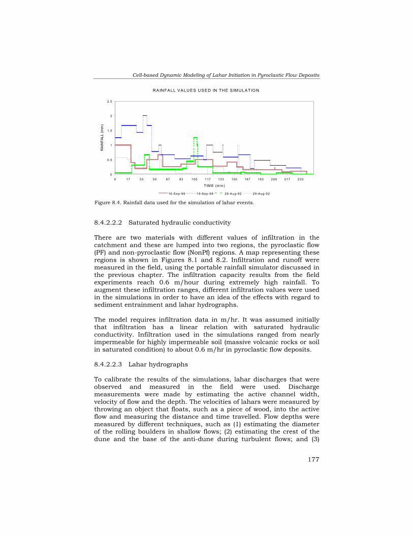
Cell-based Dynamic Modeling of Lahar Initiation in Pyroclastic Flow Deposits
177
8.4.2.2.2 Saturated hydraulic conductivity There are two materials with different values of infiltration in the catchment and these are lumped into two regions, the pyroclastic flow (PF) and non-pyroclastic flow (NonPf) regions. A map representing these regions is shown in Figures 8.1 and 8.2. Infiltration and runoff were measured in the field, using the portable rainfall simulator discussed in the previous chapter. The infiltration capacity results from the field experiments reach 0.6 m/hour during extremely high rainfall. To augment these infiltration ranges, different infiltration values were used in the simulations in order to have an idea of the effects with regard to sediment entrainment and lahar hydrographs. The model requires infiltration data in m/hr. It was assumed initially that infiltration has a linear relation with saturated hydraulic conductivity. Infiltration used in the simulations ranged from nearly impermeable for highly impermeable soil (massive volcanic rocks or soil in saturated condition) to about 0.6 m/hr in pyroclastic flow deposits. 8.4.2.2.3 Lahar hydrographs To calibrate the results of the simulations, lahar discharges that were observed and measured in the field were used. Discharge measurements were made by estimating the active channel width, velocity of flow and the depth. The velocities of lahars were measured by throwing an object that floats, such as a piece of wood, into the active flow and measuring the distance and time travelled. Flow depths were measured by different techniques, such as (1) estimating the diameter of the rolling boulders in shallow flows; (2) estimating the crest of the dune and the base of the anti-dune during turbulent flows; and (3)
Figure 8.4. Rainfall data used for the simulation of lahar events.
RAIN FA LL VALUES U SED IN TH E S IM U LATIO N
0
0.5
1
1.5
2
2.5
0 17 33 50 67 83 100 117 133 150 167 183 200 217 233
TIM E (m in)
RAI
NFA
LL (m
m)
16 -S ep-98 19-Sep-98 28-Aug-92 29-A ug-92
Chapter 8
178
making graduated markings on the opposite bank of the channel before the lahar event. Concentrations of the flow were measured using a bucket to take samples from the top portion of the active lahar flow. Concentrations of lahars were estimated by putting the sample in a clear container and allowing it to settle for a day. When settling was finished, the ratio between clear water and sediments was measured. Although the measurement of discharges and the sampling of flows are recorded at intervals, recordings are also made when there is a significant change in the flow discharges. It is assumed that in between sampling intervals there is little change in the lahar flow. The availability of the flow sensors during the lahar events served as a useful tool in determining the time, duration and magnitude of the lahar flow. Lahar hydrographs from the flow sensor data were used to fill some observation gaps in the lahar hydrograph, since the reading in the flow sensor is continuous. 8.5 The Lahar Model 8.5.1 Introduction The lahar simulation model is run entirely on PCRASTER environmental modelling software. The model is robust to operate in an environment where rapid erosion of very loose sediment occurs, capable of producing lahars. The objective was to predict a mudflow hydrograph for a designated outflow point. The model is catchment-scale and cell-based, and uses some physical laws in order to predict lahar hydrographs, taking into account the velocity, mud heights along the channel, mud concentrations and other flow properties. The cell or grid size used is 50 m and the simulation increments are in time steps (T) of five seconds. Figure 8.5 shows the general schematic diagram of the processes involved. In each time step, a new value is assigned to every cell, based on the series of equations involved in the model. The direction of the outgoing and receiving values of every cell is determined based on the LDD map.
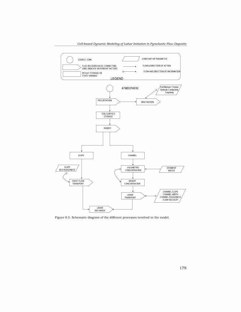
Cell-based Dynamic Modeling of Lahar Initiation in Pyroclastic Flow Deposits
179
ATMOSPHERE Soil Moisture / TextureHydraulic Conductivity
Sorpetivity
SLOPE CHANNEL
LAHARTRANSPORT
VOLUMETRICCONCENTRATION
WEIGHTCONCENTRATION
SEDIMENTWATER
CHANNEL SLOPECHANNEL WIDTH
CHANNEL ROUGHNESSFLOW VISCOSITY
LAHARDISCHARGE
SLOPEBED ROUGHNESS
SOURCE / SINK
FLUX /DECISION VALVE; CONNECTINGLINES INDICATE DEPENDENT FACTORS
RESULT STORAGE ORSTATE VARIABLE
CONSTANT OR PARAMETER
FLOW & DIRECTION OF ACTION
LEGEND
SOIL SURFACESTORAGE
PRECIPITATIONINFILTRATION
RUNOFF
SHEET FLOWTRANSPORT
FLOW AND DIRECTION OF INFORMATION
Figure 8.5. Schematic diagram of the different processes involved in the model.

Chapter 8
180
8.5.2 Input data Rainfall is assumed to be equally distributed over the catchment area. Rainfall interception was neglected since the area had nearly no vegetation at the time of the simulation. Rain was divided into time steps of five seconds.
TtssrainRain *)3600/.(= [1]
where: Rain or Pr is the amount of rainfall in m/T rain.tss = rainfall input data for one event in m/hr
T = time steps of five seconds Depending on the types of deposits, saturated hydraulic conductivity ranges from 0 to 0.02 m/hr in areas with no 1991 pyroclastic flow deposits. For the areas that have extensive 1991 pyroclastic flow deposits, input values range from 0 (fully saturated) to about 0.3 m/hr. Potential infiltration is assumed to have a linear relation with saturated hydraulic conductivity. Infiltration is calculated in two areas, i.e., on slopes and in channels. In-channel infiltration value is assumed to be zero because it is in a fully saturated condition during the simulated lahar event. Infiltration rates on slopes used different fixed values similar to hydraulic conductivity, as mentioned above. When infiltration capacity is exceeded, overland flow (runoff) is simulated. Runoff on slopes is routed into the channel. It is calculated as: H = Pr – FcA [2] where: H = height of water in slope (m/T) Pr = rainfall amount (m/T) FcA = actual infiltration (m/T) When pure rainwater falls into the channel, the volumetric concentration of the flow is diluted, and this was taken into account. 8.5.3 Transport / Routing models Two transport models were used for routing the overland flows on hill slopes and in the channel. On hill slopes, Horton overland flow is routed with the Manning equation. As regards in-channel flows for lahars, the Meunier mudflow equation is used since flow velocity is affected by mud concentration and flow volume.

Cell-based Dynamic Modeling of Lahar Initiation in Pyroclastic Flow Deposits
181
8.5.3.1 Sheet and small channel non-lahar flows Sheet flow and non-lahar channel flows are modelled using the Manning equation to calculate velocities:
NSRV )*( 2
13
2
= [3]
where: V = flow velocity (m/s) R = hydraulic radius (m) S = slope gradient (fraction) N = Manning roughness coefficient
The hydraulic radius (R ) is calculated as:
)2()(HBHBR∗+
∗= [4]
where: B = width of channel (m or pixel) H = water height in channel (m or pixel)
The mean velocity (Vmean) in a pixel is the average velocity of the central pixel and the neighbouring upper and lower pixels. 8.5.3.2 Transport model for mudflow Channel flow velocities in can start with normal stream flow, which uses the Manning equation. When a certain flow viscosity is reached that is more than 1 kNsec/m2, the Meunier flow velocity equation is used. Meunier derived the mudflow equation by conducting experiments on the behaviour of mudflow velocities with respect to rheology (Meunier, 1991). The rheology of lahars is affected by several factors, e.g., flow viscosity, volumetric concentration and weight concentration. Other factors that affect the velocity of lahars are channel slope and channel width. For the velocity of mudflow in the channel, the relationships of several rheologic aspects of the flow are incorporated in the equation. The required data were measured in the field. The Meunier equation states that:
+−=
6231 3αα
µτ hV o
Chan [5]
where: ChanV = mean velocity of mudflow in channel (m/s)
oτ = shear stress of the flow (kPa)
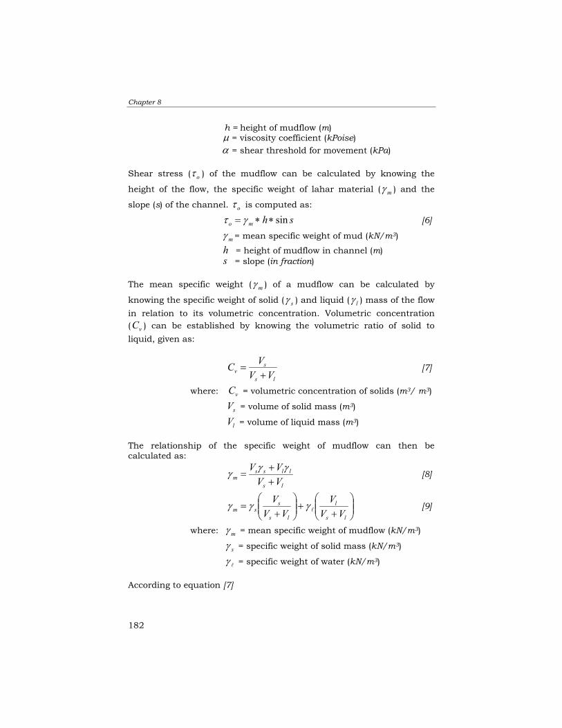
Chapter 8
182
h = height of mudflow (m) µ = viscosity coefficient (kPoise)
α = shear threshold for movement (kPa)
Shear stress ( oτ ) of the mudflow can be calculated by knowing the
height of the flow, the specific weight of lahar material ( mγ ) and the
slope (s) of the channel. oτ is computed as:
shmo sin∗∗= γτ [6]
mγ = mean specific weight of mud (kN/m3)
h = height of mudflow in channel (m) s = slope (in fraction)
The mean specific weight ( mγ ) of a mudflow can be calculated by
knowing the specific weight of solid ( sγ ) and liquid ( lγ ) mass of the flow in relation to its volumetric concentration. Volumetric concentration ( vC ) can be established by knowing the volumetric ratio of solid to liquid, given as:
ls
sv VV
VC+
= [7]
where: vC = volumetric concentration of solids (m3/ m3)
sV = volume of solid mass (m3)
lV = volume of liquid mass (m3) The relationship of the specific weight of mudflow can then be calculated as:
ls
llssm VV
VV++
=γγγ [8]
+
+
+
=ls
l
ls
ssm VV
VVV
Vlγγγ [9]
where: mγ = mean specific weight of mudflow (kN/m3)
sγ = specific weight of solid mass (kN/m3)
lγ = specific weight of water (kN/m3) According to equation [7]
Cell-based Dynamic Modeling of Lahar Initiation in Pyroclastic Flow Deposits
183
vls
s CVV
V⇒
+ and )1( v
ls
l CVV
V−⇒
+ [10]
Therefore equation [9] can be simplified as:
)1( vlvsm CC −+= γγγ [11]
Knowing the volumetric concentration of the flow, the relationship of weight concentration ( wC ) of solid to liquid could be established as:
)1( vvs
vsw CC
CC−+
=lγγ
γ [12]
where: wC = weight concentration (kN/kN)
For estimating sediment concentration in the channel and sheet erosion, the lumped model based on field measurements was used. An empirical relationship of lahar discharge and its volumetric weight was established from several field-measured lahar discharges and their corresponding volumetric weight. A regression line was fitted showing this relationship (r2 =0.89).
Qbw eaC **= [13]
where: wC = weight concentration a = constant~78.07 e = exponent b = constant~0.0057 Q = flow discharge (m³/s) Calculation of mudflow height (h) is based on mud concentration. Given
vC , the height of mudflow can be calculated given the height of water (Meunier, 1991).
v
v
l
s
CC
hh
−=
1 [14]
where: sh = fictive height of solids
lh = fictive height of liquid Fictive height of solids can be transposed to:

Chapter 8
184
−
=v
vls CChh
1 [15]
And height of mudflow (h ) can be calculated as: )( ls hhh += [16]
The Meunier equation [5] also requires the viscosity coefficient. This viscosity coefficient ( µ ) was calculated using Lee’s equation:
)2*7.79.15.2()1(* vC
vCvw C ++−−= µµ [17]
where: µ = viscosity of flow (kNsec/m2)
wµ = viscosity of pure water (kNsec/m2) Shear threshold for movement (α ) is also needed in the Meunier equation. It is calculated as:
oττα c= [18]
where: α = shear stress flow threshold
cτ = shear threshold for movement to be held constant equals to cohesion (kPa)
oτ = shear stress of the flow (kPa)
Final calculation of the total discharge (Q ) at a given time step is then calculated as: CWhVQ Chan **= [19]
where: Q = is the total discharge at given time step (m3/s)
ChanV = velocity of mudflow in channel (m/s) h = height of mudflow CW = channel width (m)

Cell-based Dynamic Modeling of Lahar Initiation in Pyroclastic Flow Deposits
185
8.6 Sensitivity analysis The different parameters that were mentioned in the model have to be tested for sensitivity in order to understand which parameters have more influence on the result. The following discussion concerns the sensitivity analysis of the model. It will be presented before showing the final results on calibration. 8.6.1 DTM: Local Drain Direction The response hydrographs generated with the model of two different time periods are significant as a result of different topographic terrain conditions and channel characteristics. The major difference in the DTMs of various periods is the change in the catchment areas. As discussed in Chapter 5 on DTM analysis, after the stream piracy event in 1993 the Pasig catchment gained an additional 20 km2, which is roughly 45% more than its original size. To demonstrate this effect on runoff, Figures 8.6 and 8.7 show the difference in total water and lahar volume between 1992 and 1998. These graphs were created by using hypothetic total rainfall events of 5 to 50 mm at 5 mm increments. In the 1992 Pasig catchment, assuming no water is lost due to infiltration, the ratio of the volume of total water collected with an increase in rainfall increases linearly at a rate of 120 times. Increase in catchment size after the 1994 capture increased the rate to about 220 times, roughly twice the 1992 catchment condition. This relationship is also portrayed in the Sacobia catchment in 1992 and in 1998. However, owing to the large catchment of Sacobia in 1992, the ratio is about 190 times. The significant reduction of catchment in 1998 reduced the capacity by about three times. The change of DTM also reflects the change in channel density and configuration. This has an enormous effect on the hydrograph with respect to lahars. This will be discussed in the next section.

Chapter 8
186
8.6.2 Channel density and channel width Another important effect of the change in DTMs is the change in channel density and geometry. The channel system in 1992 consisted of numerous densely spaced channels and gullies that were the sources of erosion and lahar transport. Compared with the DTMs used in 1998, several small gullies were interconnected, forming wider channels. This condition had an influence on the lahar delivery. To quantify this effect, an assumed total rainfall of 5, 10, 15, 25 and 50 mm in two hours were simulated. All parameters were kept equal except for the channel density and channel width. Table 8.1 gives the results of the five simulations for the three catchments. Total lahar discharge is also plotted in the Figures 8.6 and 8.7. From these figures, it can be concluded that the change in DTM conditions in 1992 and 1998 resulted in a considerable increase in the total discharge, primarily due to increase in catchment size. Peak velocity increased in the 1998 simulation, primarily due to increase in the lahar discharge. It can be further concluded that channel density is a more sensitive parameter when it comes to lahar discharge than channel width. In 1992, all catchments produced lahar volumes several orders of magnitude higher than the 1998 simulations. This occurs despite a change in the catchment area.
Figure 8.6. Simulated total lahar discharge at Pasig watershed (filled symbols in primaryleft y-axis) and total water volume (non-filled symbols on right secondary y-axis) in Pasigwatershed in 1992 and 1998 condition.
y = 120.65x
y = 220.81x
0
10000
20000
30000
40000
50000
60000
70000
80000
90000
5 10 15 20 25 30 35 40 45 50RAINFALL (mm)
TOTA
L LA
HAR
VO
LUM
E (m
3 )
0
500
1000
1500
2000
2500PASIG WATERSHED
TOTA
L W
ATER
VO
LUM
E (m
3)
Lahar 1992 Lahar 1998 Water 1992 Water 1998

Cell-based Dynamic Modeling of Lahar Initiation in Pyroclastic Flow Deposits
187
Channel width affects the velocity and height of the flow, and will therefore influence the overall response of the hydrograph. Channel width (Cw) considered in the simulation ranged from 25, 75 and 100 m for the 1992 simulations. For the 1998 simulations, channel width ranged from 100 to 200 m, owing to the channel widening in the later years after the eruption.
Figure 8.7. Simulated total lahar discharge in Sacobia watershed (filled symbols inprimary left y-axis) and total water volume (non-filled symbols on right secondary y-axis)in Pasig watershed in 1992 and 1998 condition.
y = 189.98x
y = 90.19x
0
10000
20000
30000
40000
50000
60000
70000
80000
90000
5 10 15 20 25 30 35 40 45 50RAINFALL (mm)
TOTA
L LA
HAR
VO
LUM
E (m
3 )
0
500
1000
1500
2000
2500SACOBIA WATERSHED
TOTA
L W
ATER
VO
LUM
E (m
3 )
Lahar 1992 Lahar 1998 Water 1992 Water 1998
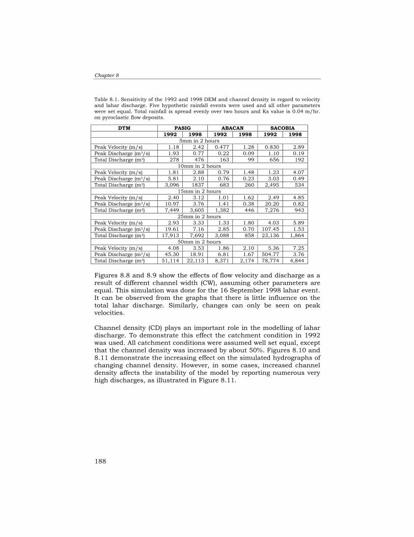
Chapter 8
188
Table 8.1. Sensitivity of the 1992 and 1998 DEM and channel density in regard to velocity and lahar discharge. Five hypothetic rainfall events were used and all other parameters were set equal. Total rainfall is spread evenly over two hours and Ks value is 0.04 m/hr. on pyroclastic flow deposits.
Figures 8.8 and 8.9 show the effects of flow velocity and discharge as a result of different channel width (CW), assuming other parameters are equal. This simulation was done for the 16 September 1998 lahar event. It can be observed from the graphs that there is little influence on the total lahar discharge. Similarly, changes can only be seen on peak velocities. Channel density (CD) plays an important role in the modelling of lahar discharge. To demonstrate this effect the catchment condition in 1992 was used. All catchment conditions were assumed well set equal, except that the channel density was increased by about 50%. Figures 8.10 and 8.11 demonstrate the increasing effect on the simulated hydrographs of changing channel density. However, in some cases, increased channel density affects the instability of the model by reporting numerous very high discharges, as illustrated in Figure 8.11.
DTM PASIG ABACAN SACOBIA 1992 1998 1992 1998 1992 1998
5mm in 2 hours Peak Velocity (m/s) 1.18 2.42 0.477 1.28 0.830 2.89 Peak Discharge (m3/s) 1.93 0.77 0.22 0.09 1.10 0.19 Total Discharge (m3) 278 476 163 99 656 192
10mm in 2 hours Peak Velocity (m/s) 1.81 2.88 0.79 1.48 1.23 4.07 Peak Discharge (m3/s) 5.81 2.10 0.76 0.23 3.03 0.49 Total Discharge (m3) 3,096 1837 683 260 2,495 534
15mm in 2 hours Peak Velocity (m/s) 2.40 3.12 1.01 1.62 2.49 4.85 Peak Discharge (m3/s) 10.97 3.76 1.41 0.38 20.20 0.82 Total Discharge (m3) 7,449 3,605 1,382 446 7,276 943
25mm in 2 hours Peak Velocity (m/s) 2.93 3.33 1.33 1.80 4.03 5.89 Peak Discharge (m3/s) 19.61 7.16 2.85 0.70 107.45 1.53 Total Discharge (m3) 17,913 7,692 3,088 858 23,136 1,864
50mm in 2 hours Peak Velocity (m/s) 4.08 3.53 1.86 2.10 5.36 7.25 Peak Discharge (m3/s) 45.30 18.91 6.81 1.67 504.77 3.76 Total Discharge (m3) 51,114 22,113 8,371 2,174 78,774 4,844

Cell-based Dynamic Modeling of Lahar Initiation in Pyroclastic Flow Deposits
189
8.6.3 Infiltration Infiltration is one of the most sensitive input variables in the simulation. It is also the most important parameter in a rainfall-runoff simulation. The infiltration condition determines the soil water capacity
LAHAR HYDROGRAPH
0200400600800
1000120014001600
0 50 100 150 200 250TIME (min)
DIS
CH
ARG
E(m
3 /s)
PASIG ABACAN SACOBIA OBSERVED (PASIG)
FLOW VELOCITY
0
1
2
3
4
5
6
7
0 50 100 150 200 250TIME (min)
VELO
CIT
Y (m
/s)
PASIG SACOBIA OBSERVED(PASIG)
Figure 8.8. 16 September 1998 simulation. Parameters Ks: Pf=0.02, Non-Pf=0.03;Cv=0.1-0.3; CW=100.
LAHAR HYDROGRAPH
0200400600800
1000120014001600
0 50 100 150 200 250TIME (min)
DIS
CH
ARG
E(m
3 /s)
PASIG ABACAN SACOBIA OBSERVED (Pasig)
FLOW VELOCITY
0
1
2
3
4
5
6
7
0 50 100 150 200 250TIME (min)
VELO
CIT
Y (m
3 /s)
PASIG SACOBIA OBSERVED(PASIG)
Figure 8.9. 16 September 1998 simulation. Parameters Ks: Pf=0.02, Non-Pf=0.03;Cv=0.1-0.3; CW=150.
LAHAR HYDROGRAPH
0200400600800
1000120014001600
0 50 100 150 200 250 300TIME (min)
DIS
CH
ARG
E(m
3 /s)
PASIG ABACAN SACOBIA OBSERVED(PASIG)
LAHAR HYDROGRAPH
0200400600800
1000120014001600
0 50 100 150 200 250TIME (min)
DIS
CH
ARG
E(m
3 )
PASIG ABACAN SACOBIA OBSERVED(PASIG)
Figure 8.10. Simulation with low channeldensity. Parameters Ks: Pf=0.2, Non-Pf=0.06; Cv=0.4-0.8; CW=100. Chapter 10
Chapter 11 Figure 8.11. Simulation withhigh channel density. Parameters Ks:Pf=0.2, Non-Pf=0.06; Cv=0.4-0.8; CW=100.

Chapter 8
190
and the amount of runoff that influences the rate of erosion in the model. Based on the observation of infiltration values from the rainfall simulations, infiltration of the different types of unsaturated deposits ranges from 0.12 to 0.6 m/hr. For the non-pyroclastic flow (NonPf) region, the infiltration values that were used ranged from 0.02 to 0.18 m/hr. For the area covered by 1991 pyroclastic flow deposits (PF), the infiltration values used range from 0.02 to 0.3 m/hr. Infiltration values above 0.3 m/hr yield low lahar discharge as compared with the actual lahars observed. The limits of the infiltration values used are lower than those that were gathered in the rainfall simulator. The high values in the rainfall simulator are due to the high rainfall intensity that was introduced - higher than that of natural rainfall. Using ranges of infiltration rates gives some insight into their effect on the lahar hydrographs. As observed in Figures 8.12 and 8.13, changing the infiltration value resulted in a higher peak discharge. 8.6.4 Initial volumetric concentration Volumetric concentration (Cv) is the ratio of water and mud in the lahar flow. This concentration of the lahar flows largely affects the transport model and volumetric lahar discharge. This parameter is directly related to the calculation of the runoff hydrograph. In this model, the input values of volumetric concentration are set to a certain range in order to control the minimum and maximum limit based on observed lahar concentrations in the field. Based on observed active lahar flows, lahar concentrations change during the flow event. This is due to complex interactions of rainfall variability, sediment supply, channel migration and many others. The lahar volumetric concentrations of lahars in 1992 and 1998 have significant differences. Lahars in 1992 are more of the hyperconcentrated to debris flow type due to abundant sediment supply upstream. Volumetric concentrations range in the order of 30 to 70%. In 1998, due to the depletion of source materials, lahars are generally more diluted and range from diluted hyperconcentrated flows to muddy stream flows. For this reason, lower volumetric concentrations are set in the simulations for 1998.

Cell-based Dynamic Modeling of Lahar Initiation in Pyroclastic Flow Deposits
191
Simulation results for the 29 August 1992 event are shown in Figures 8.14 and 8.15. Assuming all other parameters are constant and assigning different values for volumetric concentrations, the lahar hydrograph yielded different results. Figure 8.15 uses a volumetric concentration range of 0 to 80%. The model gives a relatively better fit compared with the hydrograph in Figure 8.16, which assumes a higher volumetric range value.
8.6.5 Effects of the different parameters on the hydrograph A summary of the effects of the different parameters on the output hydrographs is presented in Figure 8.16. The figure demonstrates the relative change in discharge with the three parameters in the three catchments. Volumetric concentration (Cv) is the most sensitive parameter since it controls the behaviour and quantity of the initial and the upper limit of the flow. In most cases, infiltration (Ks), channel density (CD) and saturated conductivity are the most sensitive parameters, particularly for runoff studies. Channel width (CW) is the least sensitiv among the parameters.
LAHAR HYDROGRAPH
0
100
200
300
400
500
600
0 50 100 150 200 250TIME (min)
DIS
CH
ARG
E(m
3 /s)
PASIG ABACAN SACOBIA OBSERVED(PASIG)
Chapter 12 Figure 8.12. Sept 16,1998; Ks: Pf=0.12, Non-Pf=0.2
LAHAR HYDROGRAPH
0
100
200
300
400
500
600
0 50 100 150 200 250TIME (min)
DIS
CH
ARG
E(m
3 /s)
PASIG ABACAN SACOBIA OBSERVED(PASIG)
Chapter 13 Figure 8.13. Sept 16,1998; Ks: Pf=0.06, Non-Pf=0.2
LAHAR HYDROGRAPH
0200400600800
1000120014001600
0 50 100 150 200 250TIME (min)
DIS
CH
ARG
E(m
3 /s)
PASIG ABACAN SACOBIA OBSERVED(SACOBIA)
Figure 8.14. 29 August 1992; Ks: Pf=0.2,Non-Pf=0.06, Cv=0-0.8, CW=100m
LAHAR HYDROGRAPH
0200400600800
1000120014001600
0 50 100 150 200 250 300TIME (min)
DIS
CH
ARG
E(m
3 /s)
PASIG ABACAN SACOBIA OBSERVED(SACOBIA)
Figure 8.15. 29 August 1992; Ks:Pf=0.2, Non-Pf=0.06; Cv= 0.4-0.8,CW=100m
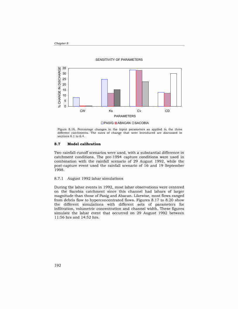
Chapter 8
192
8.7 Model calibration Two rainfall-runoff scenarios were used, with a substantial difference in catchment conditions. The pre-1994 capture conditions were used in combination with the rainfall scenario of 29 August 1992, while the post-capture event used the rainfall scenario of 16 and 19 September 1998. 8.7.1 August 1992 lahar simulations During the lahar events in 1992, most lahar observations were centered on the Sacobia catchment since this channel had lahars of larger magnitude than those of Pasig and Abacan. Likewise, most flows ranged from debris flow to hyperconcentrated flows. Figures 8.17 to 8.20 show the different simulations with different sets of parameters for infiltration, volumetric concentration and channel width. These figures simulate the lahar event that occurred on 29 August 1992 between 11:56 hrs and 14:52 hrs.
Figure 8.16. Percentage changes in the input parameters as applied in the threedifferent catchments. The rates of change that were introduced are discussed insections 6.1 to 6.4.
SENSITIVITY OF PARAMETERS
0
5
10
15
20
25
30
35
CW Ks Cv CDPARAMETERS
% C
HAN
GE
IN D
ISC
HAR
GE
PASIG ABACAN SACOBIA
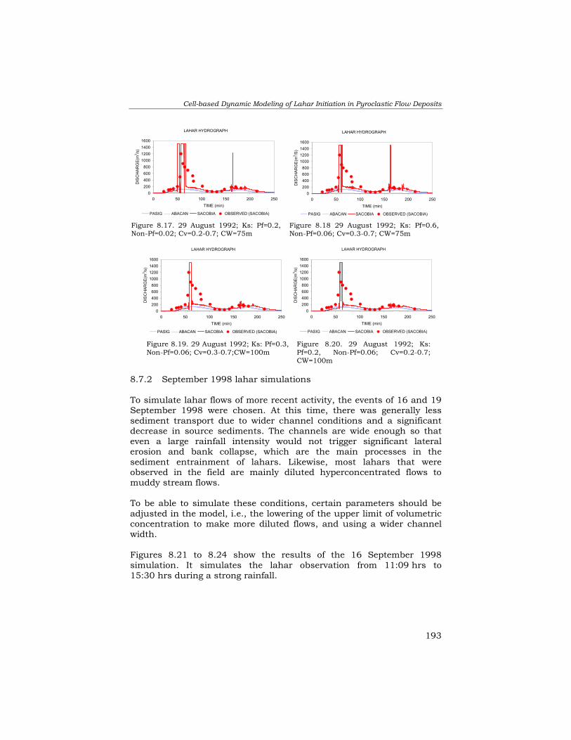
Cell-based Dynamic Modeling of Lahar Initiation in Pyroclastic Flow Deposits
193
8.7.2 September 1998 lahar simulations To simulate lahar flows of more recent activity, the events of 16 and 19 September 1998 were chosen. At this time, there was generally less sediment transport due to wider channel conditions and a significant decrease in source sediments. The channels are wide enough so that even a large rainfall intensity would not trigger significant lateral erosion and bank collapse, which are the main processes in the sediment entrainment of lahars. Likewise, most lahars that were observed in the field are mainly diluted hyperconcentrated flows to muddy stream flows. To be able to simulate these conditions, certain parameters should be adjusted in the model, i.e., the lowering of the upper limit of volumetric concentration to make more diluted flows, and using a wider channel width. Figures 8.21 to 8.24 show the results of the 16 September 1998 simulation. It simulates the lahar observation from 11:09 hrs to 15:30 hrs during a strong rainfall.
LAHAR HYDROGRAPH
0200400600800
1000120014001600
0 50 100 150 200 250TIME (min)
DIS
CH
ARG
E(m
3 /s)
PASIG ABACAN SACOBIA OBSERVED (SACOBIA)
LAHAR HYDROGRAPH
0200400600800
1000120014001600
0 50 100 150 200 250TIME (min)
DIS
CH
ARG
E(m
3 /S)
PASIG ABACAN SACOBIA OBSERVED (SACOBIA)
Figure 8.17. 29 August 1992; Ks: Pf=0.2,Non-Pf=0.02; Cv=0.2-0.7; CW=75m
Figure 8.18 29 August 1992; Ks: Pf=0.6,Non-Pf=0.06; Cv=0.3-0.7; CW=75m
LAHAR HYDROGRAPH
0200400600800
1000120014001600
0 50 100 150 200 250TIME (min)
DIS
CH
ARG
E(m
3 /s)
PASIG ABACAN SACOBIA OBSERVED (SACOBIA)
Figure 8.19. 29 August 1992; Ks: Pf=0.3,Non-Pf=0.06; Cv=0.3-0.7;CW=100m
Figure 8.20. 29 August 1992; Ks:Pf=0.2, Non-Pf=0.06; Cv=0.2-0.7;CW=100m
LAHAR HYDROGRAPH
0200400600800
1000120014001600
0 50 100 150 200 250TIME (min)
DIS
CH
ARG
E(m
3 /s)
PASIG ABACAN SACOBIA OBSERVED (SACOBIA)

Chapter 8
194
Figures 8.25 to 8.26 simulate the lahar flow that occurred on 19 September 2001 from 11:25 hrs to 11:41 hrs. The simulation was taken during a strong typhoon when precipitation was very high. In order to arrive at a reasonable simulation, a lower volumetric ratio is used, i.e., 10%, which matches the actual concentration that was observed in the field. Using a higher volumetric concentration will give a higher hydrograph, which will give poor correlation with what has been observed in the field.
LAHAR HYDROGRAPH
0100200300400500600700800
0 50 100 150 200 250TIME (min)
DIS
CH
ARG
E(m
3 /s)
PASIG ABACAN SACOBIA OBSERVED (PASIG)
Figure 8.21. 16 Sept 1998; Ks: Pf=0.18,Non-Pf=0.02; Cv=0.2; CW=CW94cut
LAHAR HYDROGRAPH
0
100
200
300
400
500
600
700
0 50 100 150 200 250TIME (min)
DIS
CH
ARG
E(m
3 /s)
PASIG ABACAN SACOBIA OBSERVED (PASIG)
Figure 8.22. 16 Sept 1998; Ks: Pf=0.03,Non-Pf=0.02; Cv=0.2; CW=CW94cut
Figure 8.23. 16 Sept 1998; Ks: Pf=0.06,Non-Pf=0.02; Cv=0.2; CW=CW94cut
LAHAR HYDROGRAPH
0
100
200
300
400
500
600
0 50 100 150 200 250TIME (min)
DIS
CH
ARG
E(m
3 /s)
PASIG ABACAN SACOBIA OBSERVED (PASIG)
LAHAR HYDROGRAPH
0
100
200
300
400
500
600
0 50 100 150 200 250TIME (min)
DIS
CH
ARG
E(m
3 /s)
PASIG ABACAN SACOBIA OBSERVED (PASIG)
Figure 8.24. 16 Sept 1998; Ks: Pf=0.12,Non-Pf=0.02; Cv=0.2; CW=CW94cut
Figure 8.25. 19 Sept 1998; Ks: Pf=0.2,Non-Pf=0.18; Cv=0.1; CW=200
LAHAR HYDROGRAPH
0
100
200
300
400
500
600
700
0 50 100 150 200 250TIME (min)
DIS
CH
ARG
E(m
3 /s)
PASIG ABACAN SACOBIA OBSERVED (PASIG)
Figure 8.26. 19 Sept 1998; Ks: Pf=0.2,Non-Pf=0.18; Cv=0.4; CW=200
LAHAR HYDROGRAPH
0
500
1000
1500
2000
2500
0 50 100 150 200 250TIME (min)
DIS
CH
ARG
E(m
3 /s)
PASIG ABACAN SACOBIA OBSERVED (PASIG)

Cell-based Dynamic Modeling of Lahar Initiation in Pyroclastic Flow Deposits
195
8.8 Conclusions Modelling rainfall-runoff on a catchment-scale can be carried out using various approaches. Simple models are generally one-dimensional, taking into account very limited parameters. More complex models that were developed involve the use of DTMs and several physical parameters for simulations. More recently, grid-based physical models were developed. Several of these catchment-scale rainfall-runoff models exist but they are generally used for agricultural and soil conservation measures. This research is among the first attempts to model rainfall runoff utilizing a cell-based distributed model, which takes into account several catchment parameters, to predict lahar runoff. In addition, this modelling approach calculates the volumetric concentration of the flows during the whole simulation period. PCRaster software, a dynamic GIS designed for environmental modelling, was used to model the lahar flows of Mt. Pinatubo. The generation of a cell-based dynamic model to simulate erosion of pyroclastic flows and lahar generation at catchment-scale for this kind of environment, involves complex procedures because of the interplay of several sensitive parameters. Routing and calculating lahar flows is complicated and involves several calculations that may make the model unstable. To minimize the instability in the model, a limited range of values was introduced for some input parameters. The physical attributes of the watersheds in the Mt. Pinatubo area changed considerably during the years after the eruption. These changes had to be incorporated in the model. They include the increase/decrease in watershed areas due to stream piracy, changes in channel density and geometry due to large-scale erosion, and changes in infiltration due to secondary pyroclastic flows or landslides. Sensitivity analysis was done to test the behaviour of the model in relation to variations of several parameters. Based on the analysis, the most sensitive parameter is the initial volumetric concentration, followed by saturated hydraulic conductivity and channel density. Channel width has little influence on the lahar hydrograph. It is recommended to calibrate several parameters after each significant change in the catchment, to obtain acceptable simulation results. It has been demonstrated that simulations of the period between 1992 and 1998 produced significant lahar magnitudes in the Sacobia and Pasig channels. The volumetric concentration of lahars largely decreased due to the depletion of source materials and the widening of channels, which made bank erosion and collapse less effective.

Chapter 8
196
The various simulations allowed to evaluate the relation between lahar discharge and rainfall amounts. Lahar hydrographs calculated by the model were compared with actual lahar hydrographs that were measured in the field. The conclusion was that the model gives reasonable estimates that can be used for lahar warning and also gives an acceptable approximation of the total sediments transported. Calculated flow velocities and the concentration of lahar flows throughout the simulation can be adopted for mitigation purposes. However, lahar flow surges observed in the field may not be well represented in the lahar model since they involve sudden fluxes in the sediment supply due to large slope failures along the channel. Although several parameters have been measured in the field, there are still some that do not reflect the exact conditions of the catchments. Since this model calculates with fairly large cells of 50 by 50 meters, in order to have acceptable calculation time, some physical attributes of the catchment had to be generalized to some extent. This simulation model is one of the few existing models that have attempted to simulate excessive erosion and lahar transportation in a volcanic setting. It is able to describe lahar flow velocity for different discharges and concentrations. There is a need to introduce an additional model component describing the frequency of bank erosion and particularly bank collapse, which delivers the sediment to the flow. This extension of the model would be a most difficult task but also highly challenging.

Conclusions and Recommendations
197
Chapter 9: Conclusions and Recommendations 9.1 Introduction A calderagenic volcanic eruption can unleash several cubic kilometres of magma and spread them as pyroclastic deposits over several hundreds of square kilometres. Such an eruption can significantly alter the topography in the watersheds surrounding the volcano. Post-eruption hazards such as lahars can be more devastating as compared to those hazards during the climactic eruption, and the threat may last for several years after the eruption. The eruption of Mt. Pinatubo in 1991 was one of the few historical cases of a calderagenic eruption. It disrupted the lives of many people and has continued to do so nearly to the present day. On the other hand, it gave many scientists from various disciplines the excellent opportunity to conduct research. In the span of a decade, numerous scientific papers have been produced that have led to a better understanding of the various phenomena related to this type of disaster. This study is focused on the post-eruption related events and contributes to a better understanding of the processes of pyroclastic flow erosion and lahar generation. Geomorphic changes were studied in a spatio-temporal context with the use of multi-date satellite images and aerial photographs. Digital Terrain Models were generated to quantify the erosion rates of the lahar source materials over the years. Hydrological properties of volcanic deposits were studied using a rainfall simulator. Rainfall-lahar threshold models were established using data from telemetered rain gauges and flow sensors, which were useful in lahar warnings. Finally, a lahar initiation and flow model was generated using dynamic GIS software to simulated short-duration lahar events. This chapter presents a synthesis and highlights the results of the different components of the research, which were initially presented in Chapter 1.4. 9.2 Research issues and main results The study of the 1991 eruption of Mt. Pinatubo and the yearly occurrences of secondary processes such as pyroclastic flow erosion and lahars, has produced several new insights into these type of hazards, which are presented below. 9.2.1 Mapping and monitoring volcanic eruption products and lahar
deposits

Chapter 9
198
Immediately after the eruption there was a huge demand for a rapid assessment of the new situation in the various watersheds surrounding the volcano. An area of about 3,000 km2 (Chapter 4.3.2) was directly affected by thick ashfall deposits, and about 200 km2 by pyroclastic flow deposits. Satellite images and vertical aerial photographs were used to rapidly assess the extent of the new deposits and evaluate the conditions of the different watersheds. The use of remote sensing technology was proven vital during the climax of the eruption on June 15-16, 1990, when the extent and magnitude of the eruption was exclusively monitored using remote sensing, as there were no direct observations possible. On the basis of the remotely sensed imagery a call was made for a total evacuation within a 40 km radius from the volcano. The use of multi-temporal remote sensing data revealed that 8 out of 15 major catchments were severely affected by pyroclastic flow deposits. Among the 8 catchments, Bucao, Marella and Sacobia-Pasig-Abacan were the most affected ones (Table 3.2). Lakes that were developed on the highly inaccessible upper slopes of the volcano were monitored using remote sensing. The main lakes that were developed were Mapanuepe, Pasig and Crater Lake, with sizes ranging from 5 to 10 km2, large enough to cause devastating lake-breakout lahars. The areas affected by lahars and siltation, with a total size of 500 km2 were rapidly mapped with the aid of remote sensing data. Though monitoring vegetation growth using NDVI maps (Figure 4.16) it can be concluded that initial vegetation growth after the eruption was limited to areas with pre-1991 pyroclastic flow deposits. Images from 1997 and 2000 showed significant vegetation growth on the upper slope of the volcano even on the 1991 pyroclastic flow deposits. In order to quantify the land cover changes, supervised classifications were carried out using all available images. One major problem encountered in the classification was the differentiation of pyroclastic flow deposits and dry lahar materials, as these two have similar spectral characteristics, and almost similar grain size distributions. In order to improve the classification, a mask outlining the area covered by pyroclastic flow deposits was used for post classification (Table 4.1). Extensive field-based mapping in accessible areas was done to collect ground truth data. Secondary explosion craters and secondary pyroclastic flow deposits, which occur in areas with thick (> 50 m) still-hot pyroclastic flow deposit, were also mapped using remote sensing. These sites were generally inaccessible and dangerous due to threat of new secondary explosions. Changes in catchment boundaries were monitored using vertical aerial photographs (see Section 9.2.3.) Although the use of satellite imagery has proven to be very useful in rapid monitoring of the impact of the Mt. Pinatubo eruption, there were also some serious limitations. For some satellite platforms, the interval

Conclusions and Recommendations
199
of satellite acquisitions for the same particular area is in the order of two to four weeks. And in practice some satellite data could only be obtained several months after acquisition. Furthermore, the Mt. Pinatubo area is mostly covered with clouds, especially during the rainy season, which makes the acquisition of cloud-free images difficult. The latter problem is overcome when using radar imagery, with which it has proven to be feasible to map wet lahar deposits. However, radar has proven to be less useful to extract information on pyroclastic flows deposits in the mountainous terrain. One other problem encountered in the monitoring of deposits through time was the incomplete scene coverage by the different images. Change detection had to be limited to the area covered by all available images. 9.2.2 Sediment budget analysis using DTMs Saturated loose volcanic deposits on the upper slopes will flow downstream as lahars. In most volcanoes, it will take several years before the source sediments will be depleted. This depletion rate is based on several factors, such as initial volume and composition of source materials, catchment configuration, amount and intensity of rainfall, and other hydrological parameters. In order to design a long-term lahar hazard mitigation plan, the annually expected sediment budget should be forecasted. In the case of Mt. Pinatubo, the initial source material erosion decay forecast curve was released during the first year after the eruption (Chapter 1.1.). It was a general erosion curve for 20 years that represented all affected watersheds. Yearly forecasts of lahar volume are known to decrease exponentially based on information from other volcanoes. Based on actual recorded events from the years following the eruption, it can be concluded that the erosion indeed followed the predicted exponential decay curve, but there were some important deviations from it in certain years due to the occurrence of “geomorphic accidents” which will be further discussed in Section 9.2.3. Calculation of the amount of erosion in the source sediments is traditionally done by mapping and quantifying the total volume of lahar deposits, which are then subtracted from the initial volume of the source sediments. This method has the advantage that lahar volume calculation can be done directly in the field. However, this method also has major drawbacks, as the analysis should include the mapping and quantification of the remaining source sediments, the geomorphic conditions of each catchment and more importantly the occurrence of stream piracy events that can effectively redistribute the remaining source sediments to another catchment. This study demonstrated that quantifying the volume of the source sediments could be achieved by using vertical aerial photographs and DTMs.

Chapter 9
200
This study quantified the amount of erosion in three watersheds located on the eastern side of the volcano, i.e., Sacobia, Pasig and Abacan. These are the most documented ones because they are located in the area with the highest population density, and the highest risk. They also experienced several cases of secondary explosions, lake breakout lahar events and stream piracies. Calculation of yearly deposition and erosion on a catchment scale was done with the aid of GIS. Twelve DTMs were available from five different organizations (Chapter 5.2). Each organization used different methods and map scales. As a consequence of that, the DTMs made by different organizations had serious discrepancies, even when they represented similar topographic areas at similar times. DTM based volumetric analysis revealed that the total volume of pyroclastic flows in the three watersheds was 1.27 km³, with 0.631 km³ in Sacobia, 0.517 km³ in Pasig and 0.128 in Abacan. Yearly estimates of the erosion rates derived from DTMs were cross-validated by comparing them with the calculated lahar deposits. Both results were of a similar order, meaning that the method was acceptable (Chapter 5.4.1 and 5.4.2). The DTMs have also been used for monitoring the spatio-temporal conditions of the different watersheds and the changes in watershed boundaries through time, which made it possible to indicate the watersheds that may produce more lahars in the following period and the areas where lahar mitigation efforts should be concentrated (Chapter 5.3.2.1). The analysis included an accuracy assessment of all the available DTMs, and the results were presented in an error matrix (Chapter 5.5.2). Misregistration errors proved to be very considerable, especially for the DTMs that were obtained without georeference. Georeferencing DTMs may suffer registration accuracies since control points are difficult to recognize and the resampling method will also have a considerable effect. Some of the available DTMs had such a low level of accuracy, that they could not be used for quantitative volumetric calculations. Among them were the DTMs produced by Jones and Newhall (dtmuspre and dtm92us) of which the resolution of 100 m was too low in comparison with the other ones, which had a 20 m resolution. The DTM that was derived from radar interferometry using TOPSAR (dtm96ts) also had large inconsistencies due to the presence of radar shadows and the poor coherence of the data. Despite the problems related to the use of secondary data, it can be concluded that DTMs are useful tools for calculating and monitoring erosion rates, for large inaccessible areas. When dealing with large-scale erosion features, the use of simple photogrammetric techniques, such

Conclusions and Recommendations
201
as height estimations using a stereoscope and parallax bar coupled with limited field checks, can give acceptable erosion estimates. Digital photogrammetrical techniques should be used for more detailed results. The most promising technique nowadays is laser altimetry, which has the capability of altitude mapping with a 15 cm vertical accuracy, which can considerably improve the accuracy of volume estimation. This technology was not used in this study since the acquisition of the data is still very costly. 9.2.3 Geomorphic accidents The term “geomorphic accidents” refers to unforeseen events that suddenly change the geomorphology of an area, and can have a serious impact on the environment. In the Mt. Pinatubo area these were mostly large secondary explosions occurring on the still-hot 1991 pyroclastic flow deposits, or massive landslides capable of eroding or burying major drainage divides. Previously, the triggering mechanism of secondary explosions was poorly understood, and it is at Mt. Pinatubo that these events were recently documented. Contributing factors are the hot temperature of pyroclastic flow deposits, thickness of the deposits, occurrence of high intensity rainfall, presence of subsurface channel water flows, and large-scale bank erosions. The occurrence of hot lahars and secondary explosions even as late as 1998 clearly showed that the pyroclastic flows, deposited in 1991, remained hot for a considerable amount of time. During the long process of cooling, these deposits are prone to secondary explosions and rapid landslides. Secondary pyroclastic flows behave similarly to vent-derived pyroclastic flows. One of the most significant effects of this process is stream piracy. The immediate effect of stream piracy is the sudden change in watershed size, and results in sudden changes of lahar activity in the affected watersheds. Such events have occurred on several occasions, such as the 4 April 1992 capture of Abacan by Sacobia, and the event of 4 October 1993 that led to the capture of upper Sacobia by the Pasig River. The April 1992 event suddenly stopped lahar activity in the Abacan River. The October 1993 event increased the Pasig catchment by 20 km² and resulted in a tremendous increase of lahar volumes in the Pasig River, from 105 million m³ in 1992 to 253 million m³ in 1993. This two-fold increase in lahar volume, caused by stream piracy, caused a temporary deviation from the exponential decay curve as mentioned in section 9.2.2. After a major volcanic eruption comparable to the one of Mt. Pinatubo, the conditions of the different watersheds should be monitored frequently. Predicting the time of occurrence of stream piracy is nearly

Chapter 9
202
impossible. However, potential sites for stream piracy can be indicated on the basis of regular updated geomorphologic maps. 9.2.4 Lahar prediction and monitoring using telemetered rain gauges
and flow sensors Lahars at Mt. Pinatubo were mostly triggered by rainfall, except for a few devastating lake breakout events. In this study, prediction and monitoring of lahars concentrated on rainfall-triggered events. Predicting lake breakout events proved to be difficult, although the magnitude of the resulting lahar can be inferred by the amount of impounded water. Rainfall triggered lahars occurred almost daily during the peak of the rainy seasons following the eruption. Visual monitoring of these events was impractical since there are eight major watersheds that produced lahar almost simultaneously, also during nighttime. Instrumental monitoring of these lahars was considered a better solution. Six rain gauges and seven flow sensors were installed in the upper part of the major watersheds around the volcano. Data from this network were received in a central computer via a telemetry system. A network of telemetered digital rain gauges and flow sensors has the advantage of recording rainfall and lahars in real time, and proved to be an important tool for lahar warning. The flow sensors give a lead-time of about 30 minutes to one hour before lahars are detected at the first lahar watch point. From there it takes about an hour or more before they reach the communities downstream. This system works day and night, a vital factor when visual observations of lahars are not possible at night or during bad weather conditions. A huge amount of data was collected over the span of 7 years. Malfunctioning instruments and interference of the transmitted data with other radio signals caused some data gaps. In order to automate the correlation of rainfall and lahars, an Excel Macro was developed to extract only the main lahar events recorded by flow sensors with at least 100 acoustic units. Likewise rainfall data that triggered lahars was only used if it had a duration between 5 and 200 minutes. Based on studies of lahars in other volcanoes, rainfall intensity and duration are considered the most important parameters for predicting the initiation of lahar flows. The relationship of rainfall intensity and duration required to trigger lahars follows a power curve. From the seven-year recordings of lahar and rainfall data, around 450 lahar events were selected. Only events with both rainfall and flow sensor data were finally selected in order to verify the timing of lahar flow, resulting in 286 events. Based on the analysis it can be concluded

Conclusions and Recommendations
203
that the rainfall intensity (I) and duration (D) required to trigger lahars varied each year. For 1991, a correlation of I = 3.2164.D -0.7397 was established, i.e., an average of about 0.26 mm/min for 30 minutes. In 1997, the average threshold increased to I = 14.523. D -0.9114, about an average of 0.65 mm/min for 30 minutes (Chapter 6.7.2.2). The increase in lahar triggering thresholds reflects the changes of the catchment conditions during various years and the depleting source sediments and changes in channel morphology. In general the yearly thresholds increased, except in 1993 due to the occurrence of a large secondary pyroclastic flow. For the seven-year period, the average threshold was I = 3.284.D -0.6443, i.e., 0.37 mm/min for 30 minutes. The flow sensors were able to record vibrations in three frequencies, i.e., low (10-100 Hz), high (100-300 Hz) and broad-band (10-300 Hz). These served as an additional tool in estimating the rheology of lahars. Debris flows and hyperconcentrated flows have a higher recording in the low frequency band, while muddy stream flows are stronger in the high frequency band. The difference in the recorded values served as the basis for distinguishing the two types of flow. The seven-year record of flow sensors showed that debris flows and hyperconcentrated flows were dominant in the initial years, and decreased significantly from late 1996 onwards, when muddy stream flow became the most frequent type. Lahar discharge or magnitude was also estimated using the flow sensor records. Flows are recorded by the sensors in terms of ground vibrations, represented as Acoustic Flow Units (AFU) in cm/sec x 10-6. A relationship of Q = 0.24.AFU was calculated for debris flows in 1992 and Q = 0.34.AFU in 1997 for muddy stream flow. These relationships of discharge and AFU are sensor specific, since the readings are affected by the distance of the sensor to the active lahar channel, and cannot be directly applied to other channels. From the analysis of the rainfall and lahar data it can be concluded that a lahar warning system cannot be based on single rainfall triggering thresholds only, as variations of threshold can vary significantly over the years. In fact a network of flow sensors coupled with manned watch points on the upper slopes will give a more reliable advance warning including information on the velocity, characteristic and magnitude of the flow.
Chapter 9
204
9.2.5 Hydraulic properties of Mt. Pinatubo deposits Hydraulic properties, such as infiltration and runoff, and their relation to slope, grain size and shear strength were investigated on-site for different deposits with the use of a portable rainfall simulator. The device was modified and calibrated to work on plots with slopes from 0 to 100%, and under rainfall intensities from 2 to 12 mm/min with duration up to several hours. Based on a large number of simulations, the following conclusions were derived. The infiltration rates of most of the deposits are very high. The infiltration shows a linear trend through time for most of the deposits. The linear trend of the cumulative infiltration graph means that the effect of sorptivity on the infiltration rate is nearly zero. This can be demonstrated by the models currently used for the cumulative infiltration, such as the Philips equation. From studying rainfall-runoff with slope variation as the main parameter, it can be concluded that on slopes of 40 to 60% the runoff is greater than on steeper slopes, i.e., 80 to 100%. This is assumed to be caused by micro-depressions or “staircase” features on steep slopes that retard the effects of runoff. Erosion results from the experiments show that rainfall intensities below 6 mm/min do not entrain significant volumes of sediment. Above this threshold collapse of sand-rich sediments in the plot leads to the accelerated contribution of sediment. Regression analysis was conducted in order to correlate infiltration and runoff with rainfall intensity, soil slope, grain size and shear strength of the deposits. The result of the analysis indicated that rainfall intensity has the highest influence. The effect of steep slopes is relatively less because it was found that slopes less than 60% produce more runoff because the material is saturated faster. The presence of finer sediments such as silt increases runoff because of lower infiltration. Rainfall simulation was also conducted in the laboratory to test the erodibility and cooling rate of the hot pyroclastic flow deposits. Samples from the field were heated to temperatures similar to those of recent pyroclastic flow deposits. The results of the simulations showed that runoff started when the temperature dropped to about 100°C, just about when the sediments began to saturate. The rainfall simulations have provided important input data for lahar modelling. However, they also have several impediments. One of the most important is the very limited size of the plot, which does not allow the inclusion of features such as overland flow from the upper slope,
Conclusions and Recommendations
205
gully formation and soil collapse in channels, which can only be studied in a large area. The resulting runoff and erosion estimates measured by the rainfall simulations are only relative indicators and should not be treated as absolute values. The transferability of the results from small plot-scale to catchment-scale is complicated and should be treated with great caution. 9.2.6 Lahar simulation modelling Most of the existing grid-based hydrological models for runoff prediction were designed for agricultural purposes predicting sediment yield in the order of few hundred tons/km²/year with watershed areas in the order of 100 km². The sediment yield at Mt. Pinatubo was calculated to be as high as 5 million tons/km²/year with catchment size of only about 40 km² (Chapter 2.2.2). Common hydrological models simulate discharge within normal stream flows using the Manning equation for routing. At Mt. Pinatubo discharge can range from muddy stream flow to debris flow in which the use of the Manning equation for routing will not be suitable. The Meunier mudflow equation was used for routing hyperconcentrated flows and debris flows. This is one of the first attempts to make a simulation model for lahars using a cell-based distributed model in a dynamic GIS. A cell-based, catchment-scale simulation of lahar flows requires several complex procedures because of the interplay of several sensitive parameters. Among these are channel width and density, infiltration capacity and volumetric concentration. In order to give a reasonable range of lahar hydrographs, these parameters should be preset to a given observed range. Lahar events that were used in the simulations represent two different lahar seasons, i.e., 1992 and 1998. Actually recorded rainfall events with a duration of about 4 hours were used for both events, as well as the resulting lahars which were continuously monitored in the field in terms of discharge, flow velocity and sediment concentrations. Both events demonstrate the effects of stream piracy that occurred in October 1993 and the change in lahar rheology from debris flow in 1992 to muddy stream flow in 1998. The August 29, 1992 simulation has a rainfall magnitude of 42 mm in 4 hours and the maximum discharge was 1,400 m3/s. While the September 19, 1998 event had a rainfall magnitude of 170 mm in 4 hours and a calculated peak discharge of 700 m3/s. The large discrepancy in discharge is caused largely by the difference in sediment concentration of the two events, i.e., more debris flow in 1992 and muddy stream flow in 1998.

Chapter 9
206
Sensitivity analysis of the input variables was conducted in order to evaluate the behaviour of these in the lahar discharge simulation model. Five parameters were tested, e.g., DTM source, channel width, infiltration, volumetric concentration of the active flow, and channel density. Among these parameters, volumetric concentration is the most sensitive since it controls the type of flow and the quantity of the initial and the upper limit of the flow. This has large effects on the 1992 simulation. Other sensitive parameters are infiltration and channel density since they have a direct influence on runoff and channel routing. Channel width is the least sensitive parameter since discharge is compensated by velocity of the flow. The model does not simulate the effect of bank erosion and collapse making the channel width parameter less sensitive. Lahar magnitude and volumetric concentrations have decreased exponentially in time as a result of sediment source depletion, channel widening, vegetation growth and the stabilization of pyroclastic flow deposits. However, this trend is interrupted when there is an occurrence of a lake breakout event or a secondary pyroclastic flow that significantly alters the watershed condition. The dynamic lahar model, which has been developed, has a number of constraints, such as: (a) Channels used in the model are assumed to have a constant
channel width. Multiple channel widths assigned to different stream orders were also simulated but resulted in some instability of the model evidenced by unrealistic fluctuations in the hydrographs.
(b) Soil collapse and bank erosion were not incorporated in the model,
due to the large complexity involved. (c) Simulating lahars with changing rheology, i.e., flow changes from
muddy stream flow to debris flow and visa versa, will require the possibility to include changing volumetric concentrations during the flow. In the model, a fixed range of threshold values was applied for simulating debris flows in order to control the instability of the model, which resulted in extremely high discharge values.
9.3 Recommendations The results of this study can be applied to other volcanoes with similar eruption characteristics. However, due to the uniqueness of Mt. Pinatubo’s watershed environments, the relationships between parameters in the model have to be studied before the model can be applied in another area. Future work has to be carried out to improve a number of issues, such as:
Conclusions and Recommendations
207
(a) The differentiation between pyroclastic flow deposits and lahars,
which exhibit similar spectral characteristics, is difficult using the classification of optical satellite data. Spectrometer measurements of these deposits may improve classification in the future. Post-classification using field knowledge will significantly improve the results.
(b) The use of secondary data, such as DTMs from different sources
entails inherent errors, such as registration and resampling errors. The accuracy of the data should be established before its possible use. It is recommended to only use DTMs that have been generated by the same method and the same accuracy standards.
(c) Thresholds for rainfall intensities and durations that trigger lahars
vary each year due to the complex interaction of the controlling factors in the watersheds. A more detailed study of the different parameters that control the thresholds should be pursued.
(d) A network of rain gauges and flow sensors gives excellent
continuous records. However, since the stations are only accessible by helicopter for maintenance purposes, there were some data gaps when the instruments were not in operation. A complete record will greatly improve the studies on rainfall-lahar thresholds.
(e) Extending the simulation duration of the lahar model is the next
important step, since this model was designed to work on short-duration lahars. This model can be extended to incorporate detailed models on sediment entrainment due to bank collapse and lateral erosion in streams, and finally on lahar accumulation.
(f) The engineering works for lahar mitigation in the form of Sabo dams
and extensive dike systems are very expensive. Several of these structures have failed in the following lahar seasons, as the designers often underestimated the volume and erosive strength of lahars. The complex behaviour of the lahar fan development has led to numerous erosion, deposition and avulsion events along several sections of the channel, making mitigation very difficult. For this reason, the far-reaching recommendation is to permanently evacuate the villages that are situated in the highest danger zones identified as a result of hazard mapping. However, such drastic measures are difficult to accept by society because people are deeply rooted in their environment, and would like to avoid inadequate evacuation centers. The government has allocated 300 million dollars for the rehabilitation of the Mt. Pinatubo area. A large part of this budget was spent on engineering mitigation structures that, to some extent proved to be ineffective.

Chapter 9
208
(g) Geomorphic accidents such as large secondary explosions causing
major stream captures were largely unrecognised before. These events should be taken into account in designing the mitigation plans with emphasis on social- and infrastructural vulnerability. Mitigation plans that are not based on sound knowledge of the terrain and are imposed too early and too quickly become inadequate because they cannot cope with a sudden shift of lahar hazards to a different watershed. Therefore such inadequate plans may waste huge amount of resources.
References
209
References
Abbott, M.B. and Refsgaard, J.C., 1996, Distributed Hydrological Modelling. Kluwer
Academic, ISBN 0-7923-4042-6, 321 p. Arboleda, R. and Martinez, M.M., 1996, 1992 Lahars in the Pasig Potrero River
System. In Newhall, C.G. and Punongbayan, R.S. (eds), Fire and Mud, Eruptions and Lahars of Mt. Pinatubo, Philippines. Quezon City/Seattle, PHIVOLCS/ University of Washington Press, p. 1045-1052.
ARCVIEW Manual, 1994, Environmental System Research Institute Inc. Arguden, T.A. and Rodolfo, K.S., 1990, Sedimentologic and Dynamic Differences
between Hot and Cold Laharic Debris Flows of Mayon Volcano, Philippines. Geological Society of America Bulletin, Vol. 102, No. 7, p. 865–876.
Atienza, G.J., 1995, Lahar Mapping Using Remote Sensing (RS) and Geographic
Information System (GIS) Techniques. MSc Thesis, International Institute for Aerospace Survey and Earth Sciences (ITC), Enschede, The Netherlands, 96 p.
Ballerini, P., Bechini, C. and Moretti, S., 1996, Experimental Activities for Soil Erosion
Evaluation and Modelling. In Slaymayer, O. (ed.), Geomorphic Hazards, 1996.
Barca, D., Crisi, G.M., Di Gregorio, S. and Nicolleta, F.P., 1993, Cellular Automata
Methods for Modelling Lava Flow: Simulation of the 1986-1987 Ethnean Eruption. Kilburn, C. and Luongo, G. (eds), Chapter 12 of Active Franas, UCL Press, London, p. 283-301.
Bautista, B.C., Bautista, M.L.P. and Garcia, D.C., 1986, Seismic Monitoring: A Useful
Tool for Mudflow Detection at Mayon Volcano, Albay, Philippines. Philippine Journal of Volcanology, Vol. 3, No. 2, p. 90-108.
Bautista, B.C., Bautista, M.L.P., Marcial, S.S., Melosantos, A.A. and Hadley, K.C.,
1991, Instrumental Monitoring of Mt. Pinatubo Lahars, Philippines [abs.]. EOS, Transactions, American Geophysical Union, Vol. 72, No. 44, p. 63.
Beasly, D.B., Huggins, L.F. and Monke, E.J., 1980. ANSWERS: A Model for Watershed
Planning. Transaction of the ASAE, Vol. 23 (1980), No. 4, p. 938-944. Beget, J.E. and Limke, A.J., 1998, Two-Dimensional Kinematic and Rheological
Modeling of the 1912 Pyroclastic Flow, Katmai, Alaska. Bulletin of Volcanology, Vol. 50, p.148-160.
Beverage, J.P. and Culbertson, J.K., 1964, Hyperconcentrations of Suspended
Sediment. American Society of Civil Engineers Proceedings, Journal of the Hydraulics Division, Vol. 90, No. HY6, p. 117-128.
Bovis, M.J. and Jakob, M., 2000, The July 29, 1998, Debris Flow and Landslide Dam
at Capricorn Creek, Mount Meager Volcanic Complex, Southern Coast Mountains, British Columbia. Canadian Journal of Earth Sciences, Vol. 37, Issue 10, p.1321-1334.
Bruinsma, J.W., 1983, Results of Potassium-argon Age Dating on Twenty Rock
Samples from the Pinatubo, Southeast Tongonan, Bacon-Manito, Southern Negros, and Tongonan, Leyte Areas, Philippines. Proprietary Report by
References
210
Robertson Research to the Philippine National Oil Company-Energy Development Corporation, 24 p.
Bubenzer, G.D., 1979, Rainfall Characteristics Important for Simulation. Proceedings
of the Rainfall Simulator Workshop, Tucson, Arizona, March 7-9, 1979. Calomarde, R.I., 1997, Lahar: An Attribute of Change in the Mophology of Sto. Tomas
– Marella River, Mt. Pinatubo, Zambales, Luzon Philippines. ITC, MSc Thesis, July 1991.
Campita, N.R., Daag, A.S., Newhall, C.G., Rowe, G. and Solidum, R.E., 1996,
Evolution of Small Crater Lake at Mt. Pinatubo. In Newhall, C.G and Punongbayan, R.S. (eds), Fire and Mud, Eruptions and Lahars of Mt. Pinatubo, Philippines. Quezon City/Seattle, PHIVOLCS/ University of Washington Press.
Castro, O.T., 1999, Potential Use of Multi-Sensor Remote Sensing for Lahar Mapping:
A Case Study in Mt. Pinatubo, Philippines. ITC MSc Thesis, 130 p. Chen, C.L., 1988a, Generalized Viscoplastic Modeling of Debris Flow. Journal
Hydraulic Engineer, Issue 114, p. 237–258. Chen, C.L., 1988b, General Solutions for Viscoplastic Debris Flow. Journal Hydraulic
Engineer, Issue 114, p. 259–282. Chorowicz, J., Lopez, E., Garcia, F., Parrot, J. F., Rudant, J. P., and Vinluan, R.,
1997, Keys to Analyze Active Lahars from Pinatubo on SAR ERS imagery. Remote Sensing of Environment, Issue 62, p. 20-29.
Costa, J.E., 1984, Physical Geomorphology of Debris Flows. In Costa, J.E. and
Fleisher, P.J. (eds), Developments and Applications of Geomorphology. Springer, Berlin, p. 268-317.
Crisi, G.M., Di Francia, A., Di Gregorion, S., Nicoletta, F., Rongo, R. and Spataro, W.,
1996, Simulation of 1991-1992 Etnean Lava Flows by Cellular Model SCIARA-2. Computational Science and Engineering, Fall 1996.
Cronin, S.J., Neall, V.E., Lecointre, J.A. and Palmer, A.S., 1995, Unusual “Snow
Slurry” Lahars from Ruapehu Volcano, New Zealand. Geology, Vol. 24, No. 12, p. 1107–1110.
Cronin, S.J., Neall, V.E., Lecointre, J.A. and Palmer, A.S., 1999, Dynamic Interactions
between Lahars and Stream Flow: A Case Study from Ruapehu Volcano, New Zealand. Geological Society of America Bulletin, Vol. 111, No. 1, p. 28–38.
Daag, A.S., 1994, Geomorphic Developments and Erosion of the Mt. Pinatubo 1991
Pyroclastic Flows in the Sacobia Watershed, Philippines. A Study Using Remote Sensing and GIS. ITC MSc Thesis, 105 p.
Daag, A.S., Dolan, M.T., Laguerta, E.P., Meeker, G.P, Newhall, C.G., Pallister, J.H. and
Solidum, R.U., 1996. Growth of a Post-Climactic Lava Dome at Mount Pinatubo, July-October 1992. In Newhall, C.G and Punongbayan, R.S. (eds), Fire and Mud, Eruptions and Lahars of Mt. Pinatubo, Philippines. Quezon City/Seattle, PHIVOLCS/ University of Washington Press, p. 647-664.
Daag, A.S., Tubianosa, B.S., Newhall, C.G., Tuñgol, N.M., Javier, D.V., Dolan, M.T., de
Los Reyes, P.J., Arboleda, R.A., Martinez, M.M. and Regalado, M.M.T., 1996, Monitoring Sulfur Dioxide Emission at Mt. Pinatubo. In Newhall, C.G and Punongbayan, R.S. (eds), Fire and Mud, Eruptions and Lahars of Mt.

References
211
Pinatubo, Philippines. Quezon City/Seattle, PHIVOLCS/ University of Washington Press, p. 409-414.
Daag, A.S. and van Westen, C.J., 1996, Cartographic Modelling of Erosion in
Pyroclastic Flow Deposits of Mt. Pinatubo, Philippines. ITC Journal, 1996-2. Daligdig, J.A., Besana, G.M. and Punongbayan, R.S., 1992, Overview and Impacts of
the 1991 Mt. Pinatubo Eruptions. Proceedings of the 4th Annual Geological Convention, 1992, Geological Society of the Philippines, p. 29-55.
Delfin, F.G., Jr., 1983, Geology of Mt. Pinatubo Geothermal Project. Philippine
National Oil Company, unpublished report, 35 p. plus figures. Delfin, F.G., Jr., Villarosa, H.G., Layugan, D.B., Clemente, V.C., Candelaria, M.R. and
Ruaya, J.R., 1996, Geothermal Exploration of the Pre-1991 Mt. Pinatubo Hydrothermal Systems. In Newhall, C.G and Punongbayan, R.S. (eds), Fire and Mud, Eruptions and Lahars of Mt. Pinatubo, Philippines. Quezon City/Seattle, PHIVOLCS/ University of Washington Press, p. 197-212.
De Roo, A.P.J., Wesseling, C.G., Cremers, N.H.D.T. and Verzandvoort, M.A., 1996,
LISEM - A Physically Based Model to Simulate Runoff and Soil Erosion in Catchments: Model Structure. In Slaymayer, O. (ed.), Geomorphic Hazards, 1996.
Di Gregorio, S., Nicoletta, F.P., Rongo, R., Sorriso-Valvo, M., Spataro, W., Spezzano, G.
and Talia, D., 1994, Landslide Simulation by Cellular Automata in Parallel Environment. Proceedings of 2nd International Workshop on Massive Parallelism: Hardware, Software and Application. October 3-7, 1994. Capri, Italy, p. 392-407.
Eleveld, M.A., 1999, Exploring Coastal Morphodynamics of Ameland (The Netherlands)
with Remote Sensing Monitoring Techniques and Dynamic Modelling in GIS, PhD Thesis, ITC Publication No. 70, ISBN 90-6461-166-7. 225 p.
Fournelle, J., Camrody, R. and Daag, A.S., 1996. Anhydrite-Bearing Pumices from the
June 15, 1991, Eruption of Mount Pinatubo. Geochemistry, Mineralogy and Petrology.
Francis, P., 1993, Volcanoes - A Planetary Perspective. Clarendon Press, 1993. ISBN 0
19 854452, 443 p. Hadley, K.C. and Lahusen, R.G., 1991, Deployment of an Acoustic Flow Monitor
System and Examples of its Application at Mt. Pinatubo, Philippines. American Geophysical Union 1991 Fall Meeting, Abstract, p. 67.
Hadley, K.C. and Lahusen, R.G., 1993, Technical Manual for Acoustic Flow Monitor.
U.S. Geological Survey, Open-file Rep. 93-xx, 19 p. Hayes, S.K., 1999, Low-Flow Sediment Transport on the Pasig-Potrero Alluvial Fan,
Mt. Pinatubo, Philippines. MSc Thesis, University of Washington, 60 p. Hayes, S.K., Montgomery, D.R. and Newhall, C.G., 2002, Fluvial Sediment Transport
and Deposition Following the 1991 Eruption of Mt. Pinatubo. Geomorphology. Vol. 45 (2002), p. 211-224.
Hoblitt, R.P., Miller, C.D. and Vallance, J.W., 1981, Origin and Stratigraphy of the
Deposit Produced by the May 18 Directed Blast. In Lipman, P.W. and
References
212
Mullineaux, D.R. (eds), The 1980 Eruptions of Mount St. Helens, Washington. U.S. Geological Survey. Professional Paper 1250, p. 401-419.
Huke, R.E., 1963, Shadows on the Land: An Economic Geography of the Philippines.
Bookmark, Manila, 428 p. IAVCEI, 1986, Understanding Volcanic Hazards Video. Produced by International
Association of Volcanology and Chemistry of the Earth's Interior (IAVCEI) and United Nations Educational Scientific and Cultural Organization (UNESCO). 24 min.
ILWIS Reference Guide, 1997, Chapter 10: Using Digital Elevation Models. Ishihara, K., Iguchi, M. and Kamo, K., 1989, Numerical Simulation of Lava Flows on
Some Volcanoes in Japan. In Fink, J.H. (ed), Lava Flows and Domes, IAVCEI Proceeding in Volcanology, Vol. 2, Springer-Verlag, New York, 1989, p. 174-207.
Iverson, R.M., Schilling, S.P. and Vallance, J.W., 1998, Objective Delineation of Areas
at Risk from Inundation by Lahars. Geological Society of America Bulletin, Vol. 110, No. 8, p. 972-984.
Janda, J.J., Daag, A.S., de los Reyes, P.J., Newhall, C.G., Pierson, T.C., Punongbayan,
R.S., Rodolfo, K.S., Solidum, R.U. and Umbal, J.V., 1996, Assessment and Response to Lahar Hazard Around Mt. Pinatubo, 1991 to 1993. In Newhall, C.G and Punongbayan, R.S. (eds), Fire and Mud, Eruptions and Lahars of Mt. Pinatubo, Philippines. Quezon City/Seattle, PHIVOLCS/ University of Washington Press, p. 107-140.
Japan International Cooperation Agency (JICA), 1996, The Study on Flood and
Mudflow Control for Sacobia-Bamban / Abacan River Draining from Mt. Pinatubo. Master Plan Study Main Report, 231 p.
Japan International Cooperation Agency (JICA), 1996, Proceedings: Seminar on Sabo
Flood Control Works (Vols 1 & 2). The Study on Flood and Mudflow Control for Sacobia – Bamban / Abacan River Draining Mt. Pinatubo
Javelosa, R., 1994, Active Quaternary Environments in the Philippine Mobile Belt.
PhD Thesis, International Institute for Aerospace Survey and Earth Sciences (ITC) Publication No. 20ISBN 90-6164—086-5, 179p.
Johnson, A.M., 1984, Debris flow, in Brunsden. In Denys, A and Prior, D.B. (eds),
Slope Instability, Wiley and Sons, Chichester, p. 257-361. Jones, J.W. and Newhall, C.G., 1996, Pre-Eruption and Post-Eruption Digital-Terrain
Models of Mt. Pinatubo. 1996. In Newhall, C.G and Punongbayan, R.S. (eds), Fire and Mud, Eruptions and Lahars of Mt. Pinatubo, Philippines. Quezon City/Seattle, PHIVOLCS/ University of Washington Press, p. 571–582.
Kamphorst, A., 1987, A Small Rainfall Simulator for the Determination of Soil
Erodibility. Department of Soil Science and Plant Nutrition, Wageningen Agricultural University, P.O. Box 8005, NL 6700 EC Wageningen, Netherlands, Journal of Agricultural Science 35 (1987) 00-00, Art. Nr. 09.06.
Karssenberg, D.J., 1996, PCRASTER Manual. Version 2. (Software by Van Duersen,
W.P.A. and Wesseling, C.G.). PCRaster Team and the Faculty of Geographical Sciences, Utrecht University, Utrecht, The Netherlands, 368 p.

References
213
Karssenberg, D.J. and the Department of Physical Geography, University of Utrecht, 1995, PCRaster Workbooks. Faculty of Geographical Sciences, University of Utrecht, Utrecht, The Netherlands.
Kerle, N., 2001, Remote Sensing Applied to the 1998 Lahar Disaster at Casita Volcano,
Nicaragua. PhD Thesis, University of Cambridge, 204 p. Kerle, N. and van Wyk de Vries, B., 2001, The 1998 Debris Avalanche at Casita
Volcano, Nicaragua: Investigation of Structural Deformation as the Cause of Slope Instability Using Remote Sensing. Journal of Volcanology and Geothermal Research, Vol. 105, Issue 1-2, p. 49-63.
Kirkby, M.J. and Cox, N.J., 1995, A Climatic Index for Soil Erosion Potential CSEP
Including Seasonal and Vegetation Factors. Catena 25, p. 333–352. Koyaguchi, T., 1996, Volume Estimation of Tephra-Fall Deposits from the June 15,
1991, Eruptions of Mt. Pinatubo by Theoretical and Geological Methods. In Newhall, C.G and Punongbayan, R.S. (eds), Fire and Mud, Eruptions and Lahars of Mt. Pinatubo, Philippines. Quezon City/Seattle, PHIVOLCS/ University of Washington Press, p. 583-600.
Kutílek, M. and Nielsen, D.R., 1994, Soil hydrology. Catena-Verlag, Cremlingen, 370 p. Lavigne, F., Thouret, J.C., Voight, B., Suwa, D. and Sumaryono, A., 1998, Lahars at
Merapi Volcano, Central Java: An Overview. Journal of Volcanology and Geothermal Research, in Voight, B. (ed.), Special Issue on Merapi Volcano.
Lavigne, F., Thouret, J.C., Voight, B., Young, K., Lahusen, R., Marso, J., Suwa, H.,
Sumaryono, A., DeJean, M. and Sayudi, D.S., 1998, Instrumental Lahar Monitoring at Merapi Volcano, Central Java, Indonesia. Journal of Volcanology and Geothermal Research, in Voight, B. (ed.), Special Issue on Merapi Volcano.
Lee, D.I. (1969) in: Van Rijn, L.C., 1993, Principles of Sediment Transport in Rivers,
Estuaries and Coastal seas. Aqua Publications, p. I-11. Levine, A.H. and Kieffer, S.W., 1991, Hydraulics of the August 7, 1980, Pyroclastic
Flow at Mount St. Helens, Washington. Geology, Vol. 19, No. 11, p. 1121–1124.
Lillesand, T.M. and Kiefer, R.W., 1987, Remote Sensing and Image Interpretation (2nd
edit.). Wiley and Sons, New York, 1987, 721 p. Lillesand, T.M. and Kiefer, R.W, 2000, Remote Sensing and Image Interpretation (4th
edit.).Wiley and Sons, New York, 2000, 724 p. Lynch, J. and Stephens, G., 1996, Mount Pinatubo: A Satellite Perspective of the June
1991 Eruptions. In Newhall, C.G and Punongbayan, R.S. (eds), Fire and Mud, Eruptions and Lahars of Mt. Pinatubo, Philippines. Quezon City/Seattle, PHIVOLCS/ University of Washington Press, p. 637-646.
Major, J.J. and Iverson, R.M., 1999, Debris-Flow Deposition: Effects of Pore-Fluid
Pressure and Friction Concentrated at Flow Margins. Geological Society of America Bulletin, Vol. 111, No. 10, p. 1424–1434.
Major, J.J., Janda, R.J. and Daag, A.S., 1996, Watershed Disturbance and Lahars on
the East Side of Mt. Pinatubo during the Mid-June 1991 Eruptions. In Newhall, C.G and Punongbayan, R.S. (eds), Fire and Mud, Eruptions and

References
214
Lahars of Mt. Pinatubo, Philippines. Quezon City/Seattle, PHIVOLCS/ University of Washington Press, p. 895-920.
Major, J.J., Pierson, T.C., Dinehart, R.L. and Costa, J.E., 2000, Sediment Yield
Following Severe Volcanic Disturbance−A Two-Decade Perspective from Mount St. Helens. Geology, Vol. 28, Issue 9, p. 819-822.
Mannaerts, C., 1992, Assessment of the Transferability of Laboratory Rainfall-Runoff and Rainfall-Soil Loss Relationships to Field and Catchment Scales. A Study in the Cape Verde Islands. PhD Thesis, University of Gent, 1992.
Marcial, S., Melosantos, A.A., Hardley, K.C., Lahusen, R.G. and Marso, J.N., 1996,
Instrumental Lahar Monitoring at Mt. Pinatubo. In Newhall, C.G and Punongbayan, R.S. (eds), Fire and Mud, Eruptions and Lahars of Mt. Pinatubo, Philippines. Quezon City/Seattle, PHIVOLCS/ University of Washington Press, p. 1015-020.
Martinez, M.M.L., Arboleda, R.A., de los Reyes, P.J., Gabinete, E. and Dolan, M.T.,
1996, Observations of 1992 Lahars along the Sacobia-Bamban River System. In Newhall, C.G and Punongbayan, R.S. (eds), Fire and Mud, Eruptions and Lahars of Mt. Pinatubo, Philippines. Quezon City/Seattle, PHIVOLCS/ University of Washington Press, p. 1033-1044.
Meunier M., 1991, Elements D'Hydraulique Torrentielle. Etudes Montagne No. 1,
Cemagref, Grenoble, 278 p. Mizuyama, T. and Yazawa, A., 1987, Computer Simulation of Debris Flow Depositional
Processes. In: Beschta T, Grant, G.E., Ice, G.G. and Swanson, F.J. (eds), Erosion and Sedimentation in the Pacific Rim. International Association of Hydrologist, Scientific Publication 165, p.179–190.
Moore, I.D., Grayson, R.B. and Ladson, A.R., 1991, Digital Terrain Modeling: A Review
of Hydrological, Geomorphological, and Biological Applications. Hydrological Processes, Vol. 5, p. 3-30.
Morgan, R.P.C., Quinton, J.N. and Rickson, R.J., 1994, Modelling Methodology for Soil
Erosion Assessment and Soil Conservation Design: The EROSEM Approach. Outlook on Agriculture, Vol. 23 (1994)1, p. 5-9.
Morgan, R.P.C., Quinton, J.N., Smith, R.E., Govers, G., Poesen, J.W.A., Auerswald, K.,
Chisci, G., Torri, D. and Styczen, M.E., 1998, The European Soil Erosion Model (EUROSEM): A Dynamic Approach for Predicting Sediment Transport from Field and Small Catchments. Earth Surface Processes and Landforms 23, p 527-544.
Mutcher, C.K., Murphree, C.E. and McGregor, K.C., 1994, Laboratory and Field Plots
for Erosion Research. In Lal, R. (ed.), Modeling Soil Erosion. Soil Erosion Research Methods (2nd edit.), 1994, ISBN 1-884015-09-3, 340 p.
Nearing, M.A., Lane, L.J. and Lopes, V.L., 1994, Modeling Soil Erosion. Soil Erosion
Research Methods (2nd edit.), 1994, ISBN 1-884015-09-3, 340 p. Newhall, C.G., Daag, A.S., Delfin, F.G., Hoblitt, R.P., McGeehin, J., Pallister, J.S.,
Regalado, M.T.R., Rubin, M., Tubianosa, B.S., Tamayo, R.A. and Umbal, J.V., 1996, Eruptive History of Mt. Pinatubo. In Newhall, C.G and Punongbayan, R.S. (eds), Fire and Mud, Eruptions and Lahars of Mt. Pinatubo, Philippines. Quezon City/Seattle, PHIVOLCS/ University of Washington Press, p. 165-198.
References
215
O’Brien, J.S., Julien, P.Y., and Fullerton, W.T., 1993, Two-Dimensional Water Flood and Mudflow Simulation. Journal Hydraulic Engineer, ASCE 119, p. 244–261.
Onstad, C.A., Radke, B.R. and Young, A., 1981, An Outdoor Portable Rainfall Erosion
Laboratory. Erosion and Sediment Transport Measurement (Proceedings of the Florence Symposium, June 1981). IAHS Publication No. 133.
Paladio-Melosantos, M.L., Solidum, R.U., Scott, W.E., Quiambao, R.B., Umbal, J.V.,
Rodolfo, K.S., Tubianosa, B.S., de Los Reyes, P.J., Alonso, R.A. and Ruelo, H.B., 1996, Tephra Fall of the 1991 Eruptions of Mt. Pinatubo, Philippines. In Newhall, C.G and Punongbayan, R.S. (eds), Fire and Mud, Eruptions and Lahars of Mt. Pinatubo, Philippines. Quezon City/Seattle, PHIVOLCS/ University of Washington Press, p. 513-536.
PCRASTER Manual, 1996. Pierson, T.C., 1998, An Empirical Method for Estimating Travel Times for Wet Volcanic
Mass Flows. Bulletin of Volcanology Vol. 60, Issue 2, p. 98-109. Pierson, T.C. and Costa, J.E., 1987, A Rheologic Classification of Subaerial Sediment-
Water Flows. Geological Society of America Reviews in Engineering Geology, Vol. 7, p. 1-12.
Pierson, T.C., Daag, A.S., de los Reyes, P.J., Regalado, M.T.M., Solidum, R.U. and
Tubianosa, B.S., 1996, Flow and Deposition of Hot lahars on the East Side of Mt. Pinatubo, July-October 1991. In Newhall, C.G and Punongbayan, R.S. (eds), Fire and Mud, Eruptions and Lahars of Mt. Pinatubo, Philippines. Quezon City/Seattle, PHIVOLCS/ University of Washington Press, p. 921-950.
Pierson, T.C., Janda, R.J., Thouret, J.C. and Borrero, C.A., 1990, Perturbation and
Melting of Snow and Ice by the 13 November 1985 Eruption of Nevado del Ruiz, Colombia, and Consequent Mobiliztion, Flow, and Deposition of Lahars. Journal of Volcanology and Geothermal Research, Vol. 41, p. 17-66.
Pierson, T.C., Janda, R.L., Umbal, J.V. and Daag, A.S., 1992, Immediate and Long-
Term Hazards and Excess Sedimentation in Rivers Draining Mt. Pinatubo, Philippines. U.S. Geological Survey Water-Resources Investigations Report 92-4039, 37 p.
Pierson, T.C. and Scott, K.M., 1985, Downstream Dilution of Lahar: Transition from
Debris Flow to Hyperconcentrated Streamflow. Water Resources Research, Vol. 21, p. 1511-1524.
Punongbayan, R.S., Newhall, C.G., Bautista, L.P., Garcia, D., Harlow, D.H., Hoblitt,
0.R.P., Sabit, J.P. and Solidum, R.U., 1996, Eruption Hazard Assessments and Warnings. In Newhall, C.G and Punongbayan, R.S. (eds), Fire and Mud, Eruptions and Lahars of Mt. Pinatubo, Philippines. Quezon City/Seattle, PHIVOLCS/ University of Washington Press, p. 67-85.
Ragan, R.M. and Jackson, T.J., 1980, Runoff Synthesis Using LANDSAT and SCS
Model. Journal of the Hydraulics Division, HY5 (1980), p. 667-679. Rodolfo, K., 1989, Origin and Early Evolution of Lahar Channel at Mabinit, Mayon
Volcano, Philippines. Geological Society of America Bulletin, Vol. 101, No. 3, p. 414–426.

References
216
Rodolfo, K.S. and Arguden, A.T., 1991, Rain-Lahar Generation and Sediment Delivery Systems at Mayon Volcano, Philippines. In Fischer, R.V. and Smith, G.A. (eds), Sedimentation in Volcanic Settings. SEPM (Society for Sedimentary Geology) Special Publication No. 45, p. 71-87.
Rodolfo, K.S., Umbal, J.V, Alonso, R.A., Remotigue, C.T., Paladio-Melosantos, M.L.O.,
Salvador, J.H.G., Evangelista, D. and Miller, Y., 1996, Two Years of Lahars on the Western Flank of Mount Pinatubo: Initiation, Flow Processes, Deposits, and Attendant Geomorphic and Hydraulic Changes. In Newhall, C.G and Punongbayan, R.S. (eds), Fire and Mud, Eruptions and Lahars of Mt. Pinatubo, Philippines, Quezon City/Seattle, PHIVOLCS/ University of Washington Press, p. 989-1013.
Savage, S.B., 1984, The Mechanics of Rapid Granular Flows, Advance Applied
Mechanic, Vol. 24, p. 289–366. Savage, S.B., 1989, Flow of Granular Materials. In Germain, P., Piau, M., Caillerie and
D. (eds), Theoretical and Applied Mechanics. Elsevier, Amsterdam, p. 241–266.
Savage, S.B., 1993, Mechanics of Debris Flows. In Hydraulic Engineering 1993,
Proceedings 1993 Conference Hydraulic Division, American Society Civil Engineers, Vol. 2, p. 1402–1407.
Savage, S.B. and Hutter, K., 1989, The Motion of a Finite Mass of Granular Material
down a Rough Incline. Journal of Fluid Mechanics, Vol. 199, p. 177–215. Savage, S.B. and Hutter, K., 1991, The Dynamics of Avalanches of Granular Materials
from Initiation to Runout. Part I. Analysis. Acta. Mech., Vol. 86, p. 201–223. Schilling, S.P., 1998, LAHARZ: GIS Programs for Automated Mapping of Lahar-
Inundation Hazards Zones. U.S. Department of the Interior, U.S. Geological Survey Open-File Report 98-638, Vancouver, Washington, 1998, 79 p.
Scott, W.E., Hoblitt, R.P., Torres, R.C., Self, S., Martinez, M.M.L. and Nillos, T., 1996,
Pyroclastic Flows of the June 15, 1991 Climactic Eruption of Mt. Pinatubo. In Newhall, C.G and Punongbayan, R.S. (eds), Fire and Mud, Eruptions and Lahars of Mt. Pinatubo, Philippines, Quezon City/Seattle, PHIVOLCS/ University of Washington Press, p. 545-570.
Scott, K.M., Janda, R.L., de la Cruz, E.G., Gabinete, E., Eto, I., Isada, M., Sexon, M.
and Hardley, K.C., 1996, Channel and Sediment Responses to Large Volumes of 1991 Volcanic Deposits on the East Flank of Mount Pinatubo. In Newhall, C.G and Punongbayan, R.S. (eds), Fire and Mud, Eruptions and Lahars of Mt. Pinatubo, Philippines, Quezon City/Seattle, PHIVOLCS/ University of Washington Press, p. 971-988.
Scrivenor, A. (1929) in Rodolfo, K., 1989, Origin and Early Evolution of Lahar Channel
at Mabinit, Mayon Volcano, Philippines. Geological Society of America Bulletin, Vol. 101, No. 3, p. 414–426.
Self, S., Zhao, J.X., Holasek, R.E., Torres, R.C. and King, A., 1996, The Atmospheric
Impact of the 1991 Mount Pinatubo. In Newhall, C.G and Punongbayan, R.S. (eds), Fire and Mud, Eruptions and Lahars of Mt. Pinatubo, Philippines, Quezon City/Seattle, PHIVOLCS/ University of Washington Press, p. 1089-1114.

References
217
Siebert, L., 1996, Hazards of Large Volcanic Debris Avalanches and Associated Eruptive Phenomena. In Scarpa, R. and Tilling, R.I. (eds), Monitoring and Mitigation of Volcano Hazards. Springer-Verlag, Berlin, p. 541–572.
Simkin, T. and Siebert, L., 1984, Explosive Eruptions in Space and Time: Duration,
Intervals, and a Comparison of the World’s Active Volcanic Belts. In Explosive Volcanism: Inception, Evolution and Hazards. National Press Academy.
Simkin, T. and Siebert, L., 1995, Volcanoes of the World. Geoscience Press, p. 165-
176. Smith, G.A. and Fritz, W.J., 1989, Volcanic Influences on Terrestrial Sedimentation.
Geology, Vol. 17, p. 375-376. Smith, G.A. and Lowe, D.R., 1991, Lahars: Volcano-Hydrologic Events and Deposition
in the Debris Flow-Hyperconcentrated Flow Continuum. Sedimentation in Volcanic Settings: SEPM Special Publication No. 45.
Sohn, Y.K., Rhee, C.W. and Kim, B.C., 1999, Debris Flow and Hyperconcentrated
Flood-Flow Deposits in an Alluvial Fan, Northwestern Part of the Cretaceous Yongdong Basin, Central Korea. Journal of Geology, Vol. 107, p.111–132.
Speight, J.C., 1974, A Parametric Approach to Landform Regions. Special Publication
of British Geographers, Vol. 7, p. 213-230. Stein, A., van der Meer, F. and Gorte, B., 1999, Spatial Statistics for Remote Sensing.
ISBN 0-7923-5978-X, 284 p. Takahashi, T., 1978, Mechanical Characteristics of Debris Flows. Journal of Hydraulic
Division, American Society Civil Engineers, Vol. 104, p. 1153–1169. Takahashi, T., 1980, Debris Flow on Prismatic Channel. Journal of Hydraulic Division,
American Society Civil Engineers, Vol. 106, p. 381–396. Thouret, J.C., Abdurachman, K.E., Bourdier, J.L. and Bronto, S., 1998, Origin,
Characteristics, and Behaviour of Lahars following the 1990 Eruption of Kelud Volcano, Eastern Java. Indonesia. Bulletin of Volcanology, Vol. 59, Issue 7, p. 460–480.
Tilling, R.I., 1989, Volcanic Hazards and their Mitigation: Progress and Problems.
Review of Geophysics, Vol. 27, No. 2, p. 237-269. Torres, R.C., 1994, Personal Communication. Torres, R., Mouginis-Mark, P., Gabreil, H., Kallianpur, K., Self, S. and Quiambao, R.,
in press, Monitoring the Evolution of the Pasig-Potrero Alluvial Fan. (forthcoming). Journal of Volcanology and Geothermal Research.
Torres, R.C., Self, S. and Martinez, M.M.L., 1996, Secondary Pyroclastic Flows from
the June 15, 1991 Ignimbrite of Mt. Pinatubo. In Newhall, C.G and Punongbayan, R.S. (eds), Fire and Mud, Eruptions and Lahars of Mt. Pinatubo, Philippines, Quezon City/Seattle, PHIVOLCS/ University of Washington Press, p. 665-678.
Tuñgol, N. and Regalado, M.T., 1996, Rainfall, Acoustic Flow Monitor Records, and
Observed Lahars of the Sacobia River in 1992. In Newhall, C.G and Punongbayan, R.S. (eds), Fire and Mud, Eruptions and Lahars of Mt. Pinatubo, Philippines, Quezon City/Seattle, PHIVOLCS/ University of Washington Press, p. 1023-1032.

References
218
Umbal, J.V. and Rodolfo, K.S., 1996, The 1991 Lahars of Southwestern Mt. Pinatubo and Evolution of the Lahar-Dammed Mapanuepe Lake. In Newhall, C.G and Punongbayan, R.S. (eds), Fire and Mud, Eruptions and Lahars of Mt. Pinatubo, Philippines, Quezon City/Seattle, PHIVOLCS/ University of Washington Press, p. 951-970.
United State Army Corps of Engineers (USACE), 1996, Mt. Pinatubo Project Report. Vallance, J.W. and Scott, K.M., 1997, The Osceola Mudflow from Mount Rainier:
Sedimentology and Hazard Implications of a Huge Clay-Rich Debris Flow. Geological Society of America Bulletin, Vol. 109, No. 2, p. 143–163.
Van Bemmelen, R.W., 1949, The Geology of Indonesia. Government Printing Office,
The Hague, Vol. IA, 732 p. Villones, R., 1980, The Aksitero Formation: Its Implications and Relationship with
Respect to the Zambales Ophiolite, Philippine Bureau of Mines and Geosciences, Technical Information Series, No. 16-80, 21 p.
Wadge, G., Young, P.A. and McKendrick, I.J., 1994, Mapping Lava Flow Hazards Using
Computer Simulation. Journal of Geophysical Research, Vol. 99, No. B1, January 10, 1994, p. 489-504.
Waythomas, F., 2000, Formation and Failure of Volcanic Debris Dams in the
Chakachatna River Valley Associated with Eruptions of the Spurr Volcanic Complex, Alaska. Geomorphology, Vol. 39, 2001, p. 111–129.
Waythomas, C.F., Walder, J.S., McGimsey, R.G. and Neal, C.A., 1996, A Catastrophic
Flood Caused by Drainage of a Caldera Lake at Aniakchak Volcano, Alaska, and Implications for Volcanic Hazards Assessment. Geological Society of America Bulletin, Boulder, Colo., Geological Society of America (GSA), Vol. 108, p. 861-871.
Whipple, K. and Dunne, T., 1992, The Influence of Debris-Flow Rheology on Fan
Morphology, Owens Valley, California. Geological Society of America Bulletin, Vol. 104, No. 7, p. 887–900.
Whiting, P.J., Stamm, J.F., Moog, D.B. and Orndorff, R.L., 1999, Sediment-
Transporting Flows in Headwater Streams. Geological Society of America Bulletin, Vol. 111, Issue 3, p. 450-466.
Wiesner, M.G and Wang, Y., 1996, Dispersal of the 1991 Tephra in the South China
Sea. In Newhall, C.G and Punongbayan, R.S. (eds), Fire and Mud, Eruptions and Lahars of Mt. Pinatubo, Philippines, Quezon City/Seattle, PHIVOLCS/ University of Washington Press, p. 537-544.
Williams, J.R., 1975, Sediment Yield Prediction with Universal Equation Using Run-
Off Factor. Present and Prospective Technology for Predicting Sediment Yield Source. U.S. Department of Agriculture, ARS-S-40, p. 244-252.
Wolfe, E.W. and Hoblitt, R.P., 1996, Overview of Eruption. In Newhall, C.G and
Punongbayan, R.S. (eds), Fire and Mud, Eruptions and Lahars of Mt. Pinatubo, Philippines, Quezon City/Seattle, PHIVOLCS/ University of Washington Press, p. 3-20.
Yokoyama, S., 1999, Rapid Formation of River Terraces in Non-Welded Ignimbrite
along the Hishida River, Kyushu, Japan. Geomorphology, Vol. 30, Issue 3, p. 291-304.

References
219
Young, R.A., Onstad, C.A., Bosch, D.D. and Anderson, W.P., 1989, AGNPS: A Nonpoint-Source Pollution Model for Evaluating Agricultural Watershed. Journal of Soil and Water Conservation, Vol. 44, No. 2, p. 168-173.

References
220

Annex A:PCRaster Script
221
Annex A: PCRaster Script PCRASTER SCRIPT for 1992 Simulation. For 1998 Simulation completely different sets of data were used. binding #Map reports DeltaHRo=deltahro; DistChan=distchan.map; VChanmean=vchan.map; Viscosity=viscos.map; Cv=cv.map; Qmud=qmud.map; H=h.map; HChan=hchan.map; Vmean=v.map; TotDischarge=totdis92.map; #outflow point map for the 3 catchments T = scalar(5); # time of one timestep (s) Area = clone92.map; # bit map covering the 3 catchments Loc = pnt92cut.map; # point map of 3 outflow points #PRECIPITATION# PI = rain92.tss; # rainfall data input (m/hour) Rain92 = rain92.map; # area map where rain should fall PStop = scalar(4.0); # duration of simulated rainstorm (hour) #MUD CHARACTERISTICS# #Specific weight of solids in mud (kN per m3) GammaSolid=18.379; #Specific weight of water in mud (kN per m3) GammaWater=10; #coefficients relating weight of solids Cw to Discharge using the equation #Qmud:Cw=a*exp(b*Qmud) a=78.07; #constant b=0.0057; #exp Qmud #Viscosity of pure water (kNsec/m2) ViscW=0.000001; #ROUTING# Ldd = ldd92cut.map; # local drain direction map N=scalar(0.04); # manning’s roughness coefficient, sheet flow CWDEF = cw92cut.map; # map depicting the actual width of channels DTM = DTM92cut.map; # elevation model BoundRou = str92cut.map; # map with stream boundaries, channels, id's

Annex A:PCRaster Script
222
areamap clone92.map;
timer 1 2160 1; #number of iterations anim=1,10+10..endtime; last=endtime;
initial PStopSec=PStop*3600; # end of rainstorm (s) PStopSt=PStopSec/T; # end of rainstorm (timesteps) #INFILTRATION# H=scalar(0); # total amount of pure water on slope(m) #ROUTING# CL=celllength(); # cell size (m) CA=cellarea(); # cellarea (m2) Channel= if(BoundRou,boolean(1),boolean(0)); # channels # distance to downstream cell (m) DCL=CL;#max(downstreamdist(Ldd),CL); # classic slope (m/m), must be larger than 0 SlopeCl=max(0.001,(slope(DTM)+upstream(Ldd,slope(DTM)) +upstream(Ldd,slope(DTM)))/3); Slope=min(0.6,SlopeCl); SinSlope=sin(atan(Slope)); #Sinus of slope SlopeSqrt=sqrt(Slope); # square root of slope TwoDivThree=2/3; # 2 divided by 3 VChanold=0; #MUDFLOW CHARACTERISTICS# Cw=0; #kg solids per m3 in mudflow mixture #Volume fraction solids in mudflow mixture Cv=0; Cvold=0; Cw = 0; HChan=scalar(0); #Initial height of water/mud in channel Viscosity=0.000001; #Viscosity in kNsec/m2 Cohesion=0; #Cohesion of mud in kPa GammaMud=GammaWater; #Gamma mud is in initial Gamma water CW= max(0.1,(CWDEF+downstream(Ldd,CWDEF))/2); #width of channel CumDischarge = 0; CumRain=0; CumInfilt=0; dynamic # PRECIPITATION # PIScalar = timeinputscalar(PI,Rain92.map); #rain per timestep (m) Rain =(PIScalar/3600)*T; #PIScalar = scalar(PI) Pr=if(time() lt PStopSt,Rain,0); # rain per timestep (m)

Annex A:PCRaster Script
223
#SATURATED CONDUCTIVITY (m/timestep)# Ks= scalar(if(Ks92cut.map == 1, 0.0130, 0.0000)); KsSt=(Ks/3600)*T; # INFILTRATION # #addition of pure water height by rain corrected for channel width DeltHrain=if (Channel,Pr,0); HChan=if(Channel,HChan+DeltHrain,0); #Correction of Cv because of addition of pure water Cv=if((HChan+DeltHrain) gt 0,(Cv*HChan)/ (HChan+DeltHrain),0); #New water height on slope by rain H=if(Channel,0,H+Pr); # potential infiltration per timestep ('rate', m/timestep) # Fc=Lineair function KsSt Fc=KsSt; # actual infiltration in channel and on slope # per timestep ('rate', m/timestep) FcA=if(Channel,0,if(H gt Fc,Fc,H)); # total amount of water on slope and channel after infiltration (m) H=if(Channel,0,max(H-FcA,0)); HChan=if(Channel,max(HChan-FcA,0),0); # ROUTING # # hydraulic radius for sheet flow R=(CL*H)/(CL+2*H); #hydraulic radius for channel flow RChan=(CW*HChan)/(CW+(2*HChan)); # flow velocity of sheetflow (m/s)# V=if(Channel,0,((R**TwoDivThree)*SlopeSqrt)/N); #mean v over three pixels Vmean=if(Channel,0,(V+upstream(Ldd,V)+downstream(Ldd,V))/3); #flow velocity in channel (m/s) #if viscosity <1 kNsec/m2 Manning else Meunier equation of mudflow ##Parameters needed for Meunier # Calculation of total shear stress (KPa) Tautot=GammaMud*HChan*SinSlope; #Calculution of alpha (Meunier equation) Alpha=Cohesion/Tautot; VChan=if(Channel,min(VChanold+0.1,if(Viscosity<1, ((RChan**TwoDivThree)*SlopeSqrt)/N,if(HChan*Alpha>=HChan,0, ((Tautot*HChan)/Viscosity)* (1/3-Alpha/2+((Alpha)**3)/6)))),0); #mean channel velocitu (vchan) over three pixels VChanmean=if(Channel,(VChan+upstream (Ldd,VChan)+downstream(Ldd,VChan))/3,0); Qmud=VChanmean*HChan*CW; #Calculation of new mud weight Cw kg/m3 empirically related to Qmud #Cw=a*exp(b*Qmud) #non cumulative Cw = Cw + (a*exp(b*Qmud)); #Calculation mudconcentration Cv m3 /m3 Cv=min(0.9,Cw*10/(GammaSolid*1000));

Annex A:PCRaster Script
224
Cv = 0.6; #in case for fix Cv #Calculation of new HChan due to new concentration of sediment HChan=if(Channel,(HChan*(1-Cvold))/(1-Cv),0); #Calculation of new viscosity in kNsec/m2 for new Cv, according to Lee Viscosity=if(Cv>0,ViscW*(1-Cv)**(-(2.5+1.9*Cv+7.7*Cv**2)),Viscosity); #Calculation of new Specific weight of mud GammaMud=GammaSolid*Cv+GammaWater*(1-Cv); # distance traveled during timestep of water/mud channel, water slope(m) Dist=if(Channel,0,Vmean*T); DistChan=if(Channel,VChanmean*T,0); ## amount of pure water(mud) that leaves the cell on slope and channel(m) #remind that Dist in channel =0 so Htr in channel= 0 HTr=(Dist/DCL)*H; HTrChan=(DistChan/DCL)*HChan; #new amount of pure water on slope m water height H=if(Channel,0,H-HTr+upstream(Ldd,HTr)); ##new amount of water/mud in channel #remind HTr is 0 in channel so channel will recieve only pure water (Htr) #from slope and HTrChan from upstream channel. #First the amount of pure water coming from the slope into the channel pixel: #with correction of channel width DeltaHRo=if(Channel,upstream(Ldd,HTr*(CL/CW)),0); #Correction of Cv because of addition of pure waterfrom run off from slopes Cv=if((HChan+DeltHrain) gt 0,(Cv*HChan)/(HChan+DeltaHRo),0); #Calculation of new hchan due to outflow and inflow in channel pixel HChan=max(0,if(Channel,Hchan- HTrChan+upstream(Ldd,HTrChan)+DeltaHRo,0)); VChanold=VChanmean; Cvold=Cv; HChanmn=(HChan+upstream(Ldd,HChan)+downstream(Ldd,HChan))/3; #BUDGET CHECK # # Total discharge in M3 per timestep at three samplepoints SumDischarge=maptotal(TotDischarge*Qmud)*T; CumDischarge=SumDischarge+CumDischarge; # Total rain per timestep in M3 RainTot=maptotal(Pr*CA); CumRain=CumRain+RainTot; #total infiltration m3 per timestep InfiltroTot=maptotal(FcA*CA); CumInfilt=CumInfilt+InfiltroTot; #total storage on slopes HTot=maptotal(H*CA); #total storage in channel HChanTot=maptotal(HChan*CW*DCL); #budget analyses per timestep. Budget=CumRain-CumInfilt-CumDischarge-HChanTot-HTot; report cumrain.tss=timeoutput(Loc,CumRain); report cuminfil.tss=timeoutput(Loc,CumInfilt); report cumdis.tss=timeoutput(Loc,CumDischarge); report htot.tss=timeoutput(Loc,HTot); report hchantot.tss=timeoutput(Loc,HChanTot); report budget.tss=timeoutput(Loc,Budget); report pr.tss=timeoutput(Loc,Pr);

Annex A:PCRaster Script
225
report qmud.tss=timeoutput(Loc,Qmud); report cv.tss=timeoutput(Loc,Cv); report cw.tss=timeoutput(Loc,Cw); report viscos.tss=timeoutput(Loc,Viscosity); report vchan.tss=timeoutput(Loc,VChanmean); report h.tss=timeoutput(Loc,H); report hchanmn.tss=timeoutput(Loc,HChanmn); report v.tss=timeoutput(Loc,Vmean); # report DeltaHRo=deltahro; report DistChan=distchan.map; # report H=h.map; # report HChan=hchan.map; report Cv=cv.map; # report Qmud=qmud.map; report VChanmean=vchan.map; # report Vmean=v.map; # report Viscosity=viscos.map; #report(anim)Qmud;

Annex A:PCRaster Script
226

Summary
227
Summary The eruption of Mt. Pinatubo in June 1991 has offered several opportunities for scientific research in various disciplines. This thesis is focused on the monitoring and modelling aspects of the erosion of pyroclastic flows and the occurrences of lahars. Monitoring the cataclysmic eruption of June 15-16, 1991 were done using satellite imageries wherein ground mapping was nearly impossible due to the widespread ashfall and the generation of large pyroclastic flows reaching up to 15 kilometres. Assessment of the yearly changes in pyroclastic flow erosion and lahar development was done using Remote Sensing (RS) and Geographic Information Systems (GIS). The eruption grossly altered eight major watersheds surrounding the volcano by depositing roughly 6.5 km³ of pyroclastic material. The Sacobia-Pasig-Abacan watersheds, with a surface of 64 km² received an initial 1.55 km³ of pyroclastic flow deposits. These watersheds have been selected for detailed studies on quantitative erosion monitoring of pyroclastic flows, determining the erosivity of the different deposits, establishing rainfall-lahar thresholds, and modelling the initiation of lahar flows. Monitoring the geomorphic changes and quantifying the erosion rate of the 1991 pyroclastic flow deposits were done using remote sensing and Geographic Information Systems (GIS). Digital Terrain Models (DTMs) were generated and were used to calculate the erosion rates and the sediment budgets. Stream piracies caused by the occurrences of secondary explosions within the thick still-hot pyroclastic flow deposits, formed a serious geomorphic threat which was previously unrecognised. These events can alter the drainage divides substantially and result in effectively gaining additional erodible pyroclastic flow deposits, and eventually shifting the catastrophic effects of lahars to the captured watershed. This has also altered the trend in the sediment budget forecast. Rain gauges and flow sensors were installed in several catchments for lahar flow warnings to the public. These instruments capture data in digital format, which were sent via telemetry and received in real time. These gave opportunities to study the lahar thresholds of several lahar events that have been recorded in a time span of 7 years. Due to the constant geomorphic changes in the watersheds after rainy seasons, the thresholds for lahar initiation also vary. As an average, a minimum rainfall of 0.33 mm/min over 30 minutes or 0.22 mm/min during 1 hour would trigger lahar flows.

Summary
228
To understand the infiltration capacity and erodibility of these deposits, a portable rainfall simulator was used in the field. Emphasis was given to the 1991 pyroclastic flow deposit since this is the main source of lahars. Simulations were conducted in order to understand the relationships of slope, grain size, infiltration and rainfall intensity in the erositivity of the deposits. Rainfall intensity is the most influential factor when it comes to erosion. The result also showed that erosion and runoff increased with decreasing slope angle since gentler slopes saturate faster. Saturation of sediments plays major role in entrenchment and collapse of deposits. Infiltration is not strongly influenced by an increase in slope steepness. Modelling of lahars using a cell-based dynamic modelling software was conducted in order to simulate short duration lahar events. The model considered several parameters including terrain, infiltration capacity, channel width, channel density and initial volumetric concentration of flows. In the model, the most sensitive parameter is volumetric concentration, followed by channel density and infiltration, while channel width is the least sensitive. The lahar model can be applied to other volcanoes with similar eruption characteristics. However, due to the uniqueness of the conditions in the Mt. Pinatubo’s are, the relationships between parameters in the model have to be studied carefully before the model can be applied elsewhere.

Summary
229
Samenvatting De vulkaan Mt. Pinatubo is gelegen op het Filippijnse eiland Luzon, ruim 100 km ten noorden van Manila. De paroxysmale eruptie van Juni 1991 heeft aanleiding gegeven tot wetenschappelijk onderzoek in vele disciplines. Dit proefschrift is gericht op het monitoren en modelleren van de erosie van pyroclastic flow afzettingen en het ontstaan van lahars. De cataclysmische eruptie vond plaats op 15 en 16 Juni 1991 en zijn effecten konden gevolgd worden met gebruik van satellietbeelden. Veldwaarnemingen waren aanvankelijk vrijwel onmogelijk door de aanwezigheid van zeer hete as en proclastic flow afzettingen die tot 15 km vanaf de krater reikten. Deze hete en losse afzettingen vormen het bronmateriaal voor vulkanische modderstromen (lahars) onder het moesson klimaat van dit gebied, dat veelvuldig door tyfoons wordt getroffen. Voor het bestuderen van de jaarlijkse verschillen in erosie van pyroclastic flow afzettingen en de ontwikkeling van lahars werd gebruik gemaakt van remote sensing en van geo-informatiesystemen (GIS). De eruptie heeft ingrijpende veranderingen teweeg gebracht in acht stroomgebieden rondom de vulkaan, door de afzetting van ongeveer 6.5 kubieke kilometer pyroclastisch materiaal. De Sacobia-Pasig-Abacan stroomgebieden met een oppervlak van 64 km2 ontvingen aanvankelijk 1.55 km3 pyroclastic flow afzettingen. Dit gebied is geselecteerd voor gedetailleerde kwantitatieve erosie monitoring op pyroclastic flows, waarbij de erodibiliteit van de verschillende afzettingen is bepaald, de regenval-lahar drempelwaarden zijn berekend, en het ontstaan van lahars is gemodelleerd. Het monitoren van de geomorfologische veranderingen en het kwantificeren van de erosiewaarden van de 1991 pyroclastic flow afzettingen werd gedaan met behulp van remote sensing en GIS. Digitale terreinmodellen (DTM’s) werden gegenereerd en gebruikt om de erosiewaarden en de sedimentbudgetten te berekenen. Stroomonthoofdingen die plaats vonden als gevolg van secondaire stoomexplosies in de dikke en nog hete pyroclastic flow afzettingen, vormden een ernstig geomorfologisch gevaar dat voordien niet herkend was. Hierdoor worden waterscheidingen verlegd waardoor andere erodeerbare pyroclastic flow afzettingen als bron gaan fungeren voor catastrofale lahars in het rovende stroomgebied. Dit betekent een onvoorzienbare verandering in de lahar-intensiteit: in het ene stroomgebied treden ze onverwachts op of verhevigen onverwachts, in het ander stroomgebied nemen ze onverwachts af. Dit heeft ook

Summary
230
veranderingen in de tendens van het verwachte sediment budget tot gevolg. Regenmeters en stroomsensors werden geïnstalleerd in verscheidene stroomgebieden om lahar waarschuwingen aan het publiek mogelijk te maken. Deze instrumenten nemen gegevens op in digitaal formaat, die via telemetrie in real-time werden ontvangen. Dit gaf mogelijkheden om de lahar drempelwaarden van diverse lahar gebeurtenissen te bestuderen, die over een periode van 7 jaar zijn geregistreerd. Door de constante geomorfologische veranderingen in het stroomgebied na het regenseizoen, varieert ook de drempelwaarde voor lahar initiatie. Als gemiddelde kan worden gesteld dat regenval van tenminste 0.33 mm/min over 30 minuten, of 0.22 mm/min met minimum duur van 1 uur, laharstromen laat ontstaan. Om de infiltratiecapaciteit en erodibiliteit van deze afzettingen te bestuderen, werd een draagbare regenvalsimulator in het veld gebruikt. Nadruk werd gelegd op de 1991 pyroclastic flow afzettingen omdat deze de hoofdbron van lahars zijn. De simulaties werden uitgevoerd om inzicht te krijgen in de verbanden tussen hellingshoek, korrelgrootte, infiltratie en regenvalintensiteit en de erodeerbaarheid van de afzettingen. Als het op erosie aankomt, is regenvalintensiteit de belangrijkste factor. Echter, erosie en afstroming nemen ook toe met afnemende hellingshoeken omdat geringere hellingen sneller verzadigd raken. Verzadiging van sedimenten speelt een belangrijke rol in de insnijding en instorting van afzettingen. Infiltratie wordt niet sterk beïnvloed door een toename in steilheid van de helling. Het modelleren van lahars met gebruik van een cell-based dynamisch modelleer softwarepakket werd gedaan om lahars van korte duur te simuleren. Het model beschouwde diverse parameters waaronder terrein, infiltratiecapaciteit, kanaalbreedte, kanaaldiepte en initiële volumetrische concentratie van stromen. In het model zijn de gevoeligste parameters: volumetrische concentraties, gevolgd door kanaaldichtheid en dan infiltratie, terwijl kanaalbreedte de minst gevoelige is. Het ontwikkelde lahar model kan worden toegepast op vulkanen met vergelijkbare condities. Echter, vanwege het unieke karakter van het Pinatubo gebied, moeten de relaties tussen de verschillende model parameters eerst onderzocht worden voordat het model elders wordt toegepast.

Summary
231
Curriculum vitae Arturo Santos Daag was born in 14 August 1962 in San Miguel, Betis, Guagua, Pampanga, Philippines. He graduated in Geology at the Mapua Institute of Technology in Manila in 1984. He continued his career by entering the Master of Science Program in Geology at the University of the Philippines in 1987. After a year in the University, he went to Enschede, the Netherlands to attend the 11-month Post-Graduate Diploma Course in Applied Geomorphology and Engineering Geology at the International Institute for Aerospace Survey and Earth Sciences (ITC). In 1994 he continued his study and was awarded Master of Science in Applied Geomorphology at ITC, Enschede. His MSc. thesis title was “Modelling Pyroclastic Flow Erosion of Mt. Pinatubo, Philippines”. Mr. Daag currently works as a Supervising Science Research Specialist at the Philippine Institute of Volcanology and Seismology (PHIVOLCS) under the Department of Science and Technology (DOST). He has been involved extensively in the study of Mt. Pinatubo during the pre-eruption monitoring and the study of lahars for several years after the eruption. His research on Mt. Pinatubo gave him the opportunity to present his work in several international conferences. He is also a major contributor to the book on “Fire and Mud: Eruption and Lahars of Mt. Pinatubo, Philippines.”

Summary
232

ITC Dissertation List
233
ITC DISSERTATION LIST 1. Akinyede, 1990, Highway cost modelling and route selection
using a geotechnical information system 2. Pan He Ping, 1990, 90-9003757-8, Spatial structure theory in
machine vision and applications to structural and textural analysis of remotely sensed images
3. Bocco Verdinelli, G., 1990, Gully erosion analysis using remote sensing and geographic information systems: a case study in Central Mexico
4. Sharif, M, 1991, Composite sampling optimization for DTM in the context of GIS
5. Drummond, J., 1991, Determining and processing quality parameters in geographic information systems
6. Groten, S., 1991, Satellite monitoring of agro-ecosystems in the Sahel
7. Sharifi, A., 1991, 90-6164-074-1, Development of an appropriate resource information system to support agricultural management at farm enterprise level
8. Zee, D. van der, 1991, 90-6164-075-X, Recreation studied from above: Air photo interpretation as input into land evaluation for recreation
9. Mannaerts, C., 1991, 90-6164-085-7, Assessment of the transferability of laboratory rainfall-runoff and rainfall - soil loss relationships to field and catchment scales: a study in the Cape Verde Islands
10. Ze Shen Wang, 1991: 90-393-0333-9, An expert system for cartographic symbol design
11. Zhou Yunxian, 1991, 90-6164-081-4, Application of Radon transforms to the processing of airborne geophysical data
12. Zuviria, M. de, 1992, 90-6164-077-6, Mapping agro-topoclimates by integrating topographic, meteorological and land ecological data in a geographic information system: a case study of the Lom Sak area, North Central Thailand
13. Westen, C. van, 1993, 90-6164-078-4, Application of Geographic Information Systems to landslide hazard zonation
14. Shi Wenzhong, 1994, 90-6164-099-7, Modelling positional and thematic uncertainties in integration of remote sensing and geographic information systems
15. Javelosa, R., 1994, 90-6164-086-5, Active Quaternary environments in the Philippine mobile belt
16. Lo King-Chang, 1994, 90-9006526-1, High Quality Automatic DEM, Digital Elevation Model Generation from Multiple Imagery

Summary
234
17. Wokabi, S., 1994, 90-6164-102-0, Quantified land evaluation for maize yield gap analysis at three sites on the eastern slope of Mt. Kenya
18. Rodriguez, O., 1995, Land Use conflicts and planning strategies in urban fringes: a case study of Western Caracas, Venezuela
19. Meer, F. van der, 1995, 90-5485-385-9, Imaging spectrometry & the Ronda peridotites
20. Kufoniyi, O., 1995, 90-6164-105-5, Spatial coincidence: automated database updating and data consistency in vector GIS
21. Zambezi, P., 1995, Geochemistry of the Nkombwa Hill carbonatite complex of Isoka District, north-east Zambia, with special emphasis on economic minerals
22. Woldai, T., 1995, The application of remote sensing to the study of the geology and structure of the Carboniferous in the Calañas area, pyrite belt, SW Spain
23. Verweij, P., 1995, 90-6164-109-8, Spatial and temporal modelling of vegetation patterns: burning and grazing in the Paramo of Los Nevados National Park, Colombia
24. Pohl, C., 1996, 90-6164-121-7, Geometric Aspects of Multisensor Image Fusion for Topographic Map Updating in the Humid Tropics
25. Jiang Bin, 1996, 90-6266-128-9, Fuzzy overlay analysis and visualization in GIS
26. Metternicht, G., 1996, 90-6164-118-7, Detecting and monitoring land degradation features and processes in the Cochabamba Valleys, Bolivia. A synergistic approach
27. Hoanh Chu Thai, 1996, 90-6164-120-9, Development of a Computerized Aid to Integrated Land Use Planning (CAILUP) at regional level in irrigated areas: a case study for the Quan Lo Phung Hiep region in the Mekong Delta, Vietnam
28. Roshannejad, A., 1996, 90-9009284-6, The management of spatio-temporal data in a national geographic information system
29. Terlien, M., 1996, 90-6164-115-2, Modelling Spatial and Temporal Variations in Rainfall-Triggered Landslides: the integration of hydrologic models, slope stability models and GIS for the hazard zonation of rainfall-triggered landslides with examples from Manizales, Colombia
30. Mahavir, J., 1996, 90-6164-117-9, Modelling settlement patterns for metropolitan regions: inputs from remote sensing
31. Al-Amir, S., 1996, 90-6164-116-0, Modern spatial planning practice as supported by the multi-applicable tools of remote sensing and GIS: the Syrian case
32. Pilouk, M., 1996, 90-6164-122-5, Integrated modelling for 3D GIS 33. Duan Zengshan, 1996, 90-6164-123-3, Optimization modelling of
a river-aquifer system with technical interventions: a case study for the Huangshui river and the coastal aquifer, Shandong, China

ITC Dissertation List
235
34. Man, W.H. de, 1996, 90-9009-775-9, Surveys: informatie als norm: een verkenning van de institutionalisering van dorp - surveys in Thailand en op de Filippijnen
35. Vekerdy, Z., 1996, 90-6164-119-5, GIS-based hydrological modelling of alluvial regions: using the example of the Kisaföld, Hungary
36. Pereira, Luisa, 1996, 90-407-1385-5, A Robust and Adaptive Matching Procedure for Automatic Modelling of Terrain Relief
37. Fandino Lozano, M., 1996, 90-6164-129-2, A Framework of Ecological Evaluation oriented at the Establishment and Management of Protected Areas: a case study of the Santuario de Iguaque, Colombia
38. Toxopeus, B., 1996, 90-6164-126-8, ISM: an Interactive Spatial and temporal Modelling system as a tool in ecosystem management: with two case studies: Cibodas biosphere reserve, West Java Indonesia: Amboseli biosphere reserve, Kajiado district, Central Southern Kenya
39. Wang Yiman, 1997, 90-6164-131-4, Satellite SAR imagery for topographic mapping of tidal flat areas in the Dutch Wadden Sea
40. Saldana-Lopez, Asunción, 1997, 90-6164-133-0, Complexity of soils and Soilscape patterns on the southern slopes of the Ayllon Range, central Spain: a GIS assisted modelling approach
41. Ceccarelli, T., 1997, 90-6164-135-7, Towards a planning support system for communal areas in the Zambezi valley, Zimbabwe; a multi-criteria evaluation linking farm household analysis, land evaluation and geographic information systems
42. Peng Wanning, 1997, 90-6164-134-9, Automated generalization in GIS
43. Lawas, C., 1997, 90-6164-137-3, The Resource Users' Knowledge, the neglected input in Land resource management: the case of the Kankanaey farmers in Benguet, Philippines
44. Bijker, W., 1997, 90-6164-139-X, Radar for rain forest: A monitoring system for land cover Change in the Colombian Amazon
45. Farshad, A., 1997, 90-6164-142-X, Analysis of integrated land and water management practices within different agricultural systems under semi-arid conditions of Iran and evaluation of their sustainability
46. Orlic, B., 1997, 90-6164-140-3, Predicting subsurface conditions for geotechnical modelling
47. Bishr, Y., 1997, 90-6164-141-1, Semantic Aspects of Interoperable GIS
48. Zhang Xiangmin, 1998, 90-6164-144-6, Coal fires in Northwest China: detection, monitoring and prediction using remote sensing data

Summary
236
49. Gens, R., 1998, 90-6164-155-1, Quality assessment of SAR interferometric data
50. Turkstra, J., 1998, 90-6164-147-0, Urban development and geographical information: spatial and temporal patterns of urban development and land values using integrated geo-data, Villaviciencia, Colombia
51. Cassells, C., 1998, Thermal modelling of underground coal fires in northern China
52. Naseri, M., 1998, 90-6164-195-0, Characterization of Salt-affected Soils for Modelling Sustainable Land Management in Semi-arid Environment: a case study in the Gorgan Region, Northeast, Iran
53. Gorte B.G.H., 1998, 90-6164-157-8, Probabilistic Segmentation of Remotely Sensed Images
54. Tenalem Ayenew, 1998, 90-6164-158-6, The hydrological system of the lake district basin, central main Ethiopian rift
55. Wang Donggen, 1998, 90-6864-551-7, Conjoint approaches to developing activity-based models
56. Bastidas de Calderon, M., 1998, 90-6164-193-4, Environmental fragility and vulnerability of Amazonian landscapes and ecosystems in the middle Orinoco river basin, Venezuela
57. Moameni, A., 1999, Soil quality changes under long-term wheat cultivation in the Marvdasht plain, South-Central Iran
58. Groenigen, J.W. van, 1999, 90-6164-156-X, Constrained optimisation of spatial sampling: a geostatistical approach
59. Cheng Tao, 1999, 90-6164-164-0, A process-oriented data model for fuzzy spatial objects
60. Wolski, Piotr, 1999, 90-6164-165-9, Application of reservoir modelling to hydrotopes identified by remote sensing
61. Acharya, B., 1999, 90-6164-168-3, Forest biodiversity assessment: A spatial analysis of tree species diversity in Nepal
62. Akbar Abkar, Ali, 1999, 90-6164-169-1, Likelihood-based segmentation and classification of remotely sensed images
63. Yanuariadi, T., 1999, 90-5808-082-X, Sustainable Land Allocation: GIS-based decision support for industrial forest plantation development in Indonesia
64. Abu Bakr, Mohamed, 1999, 90-6164-170-5, An Integrated Agro-Economic and Agro-Ecological Framework for Land Use Planning and Policy Analysis
65. Eleveld, M., 1999, 90-6461-166-7, Exploring coastal morphodynamics of Ameland (The Netherlands) with remote sensing monitoring techniques and dynamic modelling in GIS
66. Yang Hong, 1999, 90-6164-172-1, Imaging Spectrometry for Hydrocarbon Microseepage
67. Mainam, Félix, 1999, 90-6164-179-9, Modelling soil erodibility in the semiarid zone of Cameroon

ITC Dissertation List
237
68. Bakr, Mahmoud, 2000, 90-6164-176-4, A Stochastic Inverse-Management Approach to Groundwater Quality
69. Zlatanova, Z., 2000, 90-6164-178-0, 3D GIS for Urban Development
70. Ottichilo, Wilber K., 2000, 90-5808-197-4, Wildlife Dynamics: An Analysis of Change in the Masai Mara Ecosystem
71. Kaymakci, Nuri, 2000, 90-6164-181-0, Tectono-stratigraphical Evolution of the Cankori Basin (Central Anatolia, Turkey)
72. Gonzalez, Rhodora, 2000, 90-5808-246-6, Platforms and Terraces: Bridging participation and GIS in joint-learning for watershed management with the Ifugaos of the Philippines
73. Schetselaar, Ernst, 2000, 90-6164-180-2, Integrated analyses of granite-gneiss terrain from field and multisource remotely sensed data. A case study from the Canadian Shield
74. Mesgari, Saadi, 2000, 90-3651-511-4, Topological Cell-Tuple Structure for Three-Dimensional Spatial Data
75. Bie, Cees A.J.M. de, 2000, 90-5808-253-9, Comparative Performance Analysis of Agro-Ecosystems
76. Khaemba, Wilson M., 2000, 90-5808-280-6, Spatial Statistics for Natural Resource Management
77. Shrestha, Dhruba, 2000, 90-6164-189-6, Aspects of erosion and sedimentation in the Nepalese Himalaya: highland-lowland relations
78. Asadi Haroni, Hooshang, 2000, 90-6164-185-3, The Zarshuran Gold Deposit Model Applied in a Mineral Exploration GIS in Iran
79. Raza, Ale, 2001, 90-3651-540-8, Object-oriented Temporal GIS for Urban Applications
80. Farah, Hussein, 2001, 90-5808-331-4, Estimation of regional evaporation under different weather conditions from satellite and meteorological data. A case study in the Naivasha Basin, Kenya
81. Zheng, Ding, 2001, 90-6164-190-X, A Neural - Fuzzy Approach to Linguistic Knowledge Acquisition and Assessment in Spatial Decision Making
82. Sahu, B.K., 2001, Aeromagnetics of continental areas flanking the Indian Ocean; with implications for geological correlation and Gondwana reassembly
83. Alfestawi, Y., 2001, 90-6164-198-5, The structural, paleogeographical and hydrocarbon systems analysis of the Ghadamis and Murzuq Basins, West Libya, with emphasis on their relation to the intervening Al Qarqaf Arch
84. Liu, Xuehua, 2001, 90-5808-496-5, Mapping and Modelling the Habitat of Giant Pandas in Foping Nature Reserve, China
85. Oindo, Boniface Oluoch, 2001, 90-5808-495-7, Spatial Patterns of Species Diversity in Kenya
86. Carranza, Emmanuel John, 2002, 90-6164-203-5, Geologically-constrained Mineral Potential Mapping

Summary
238
87. Rugege, Denis, 2002, 90-5808-584-8, Regional Analysis of Maize-Based Land Use Systems for Early Warning Applications
88. Liu, Yaolin, 2002, 90-5808-648-8, Categorical Database Generalization in GIS
89. Ogao, Patrick, 2002, 90-6164-206-X, Exploratory Visualization of Temporal Geospatial Data using Animation
90. Abadi, Abdulbaset M., 2002, 90-6164-205-1, Tectonics of the Sirt Basin – Inferences from tectonic subsidence analysis, stress inversion and gravity modelling
91. Geneletti, Davide, 2002, 90-5383-831-7, Ecological Evaluation for Environmental Impact Assessment
92. Sedogo, Laurent G., 2002, 90-5808-751-4, Integration of Participatory Local and Regional Planning for Resources Management using Remote Sensing and GIS
93. Montoya, Lorena, 2002, 90-6164-208-6, Urban Disaster Management: a case study of earthquake risk assessment in Carthago, Costa Rica
94. Ahmad, Mobin-ud-Din, 2002, 90-5808-761-1, Estimation of Net Groundwater Use in Irrigated River Basins using Geo-information Techniques: A case study in Rechna Doab, Pakistan
95. Said, Mohammed Yahya, 2003, 90-5808-794-8, Multiscale perspectives of species richness in East Africa
96. Schmidt, Karin, 2003, 90-5808-830-8, Hyperspectral Remote Sensing of Vegetation Species Distribution in a Saltmarsh
97. Lopez Binnquist, Citlalli, 2003, 90-3651-900-4, The Endurance of Mexican Amate Paper: Exploring Additional Dimensions to the Sustainable Development Concept
98. Huang, Zhengdong, 2003, 90-6164-211-6, Data Integration for Urban Transport Planning
99. Cheng, Jianquan, 2003, 90-6164-212-4, Modelling Spatial and Temporal Urban Growth
100. Campos dos Santos, Jose Laurindo, 2003, 90-6164-214-0, A Biodiversity Information System in an Open Data/Metadatabase Architecture
101. Hengl, Tomislav, 2003, 90-5808-896-0, PEDOMETRIC MAPPING, Bridging the gaps between conventional and pedometric approaches
102. Barrera Bassols, Narciso, 2003, 90-6164-217-5, Symbolism, Knowledge and management of Soil and Land Resources in Indigenous Communities: Ethnopedology at Global, Regional and Local Scales
103. Zhan, Qingming, 2003, 90-5808-917-7, A Hierarchical Object-Based Approach for Urban Land-Use Classification from Remote Sensing Data