Embed Size (px)
Citation preview
49
MODELLING OF SELECTION AND MATING DECISIONS INTREE BREEDING PROGRAMS
Hardwood trees from the temperate forests of southern Australia arean important source of timber for high quality paper. Two species inparticular, Eucalyptus globulus and Eucalyptus nitens are well suitedto this purpose and are now widely grown in commercial plantations.These plantations have been established by professional tree breed-ers using seedlings derived originally from broadly based collectionof seed in natural forests. To increase productivity it is desirableto select trees that grow quickly and give high yields of top qualitytimber. Nevertheless it is important to maintain genetic diversityin the breeding population and thereby retain a robust capacity toadapt to changing environmental factors. In this article we formu-late a number of related mathematical models for the selection andmating processes and discuss the consequences of these models. Werecommend a relatively simple scheme which can be implemented onan IBM compatible PC using standard algorithms.
1. Introduction
Tree breeding aims to maximise the rate of genetic progress with each gener-ation. To achieve this goal, tree breeders have to take a number of key decisions:
• which of the available trees should be selected for use in the breedingprogram;
• to what extent should each selected tree contribute to the next generation;and
• which mate pairs should be used.
After a brief review of relevant literature (Brisbane and Gibson, 1995; Jansenand Wilt on, 1985; Meuwissen and Woolliams, 1994; and Sedgley and Griffin,1989) and discussion with representatives from the Cooperative Research Cen-tre in Temperate Hardwood Forestry, the Southern Tree Breeding Associationand Northern Forest Products, the MISG team suggested three alternative mod-els. The basic tree selection model was developed in detail and a correspondingselection scheme has already been implemented using real data. This schemewill
50 eRe in Temperate Hardwood Forestry
• select the number of times each tree should be mated in order to maximisethe total breeding value of the selected trees subject to an appropriatepenalty for their collective pairwise relatedness.
Two other models were developed in principle. The entropy model makes noveluse of a standard entropy function to measure the genetic diversity of the breed-ing population and a corresponding scheme would
• select the number of times each tree should be mated in order to maximisethe entropy of the selected trees while maintaining an acceptable totalbreeding value.
The third model is more complicated but may be useful in the longer termto predict the improvement in breeding values over a number of generations.In recognizing that the breeding value for the progeny of a particular matingis a random variable with expected value equal to the average breeding valueof the parents the MISG team realised that if a large number of progeny areproduced from each particular cross and only the best progeny are selected thenthe expected breeding value of the selected progeny will be somewhat higherthan the average breeding value of the parents. The enhanced tree selectionmodel incorporates these ideas and a corresponding scheme would
• calculate the number of progeny to be produced and the minimum accept-able breeding value for each cross in order to maximise the total expectedbreeding value for the selected progeny subject to the incorporation ofsufficient genetic diversity in the progeny.
2. Measuring the genetic content of a population
We suppose the current population 'Pt at time t is descended from an originalpopulation 'Po of N individuals denoted by aba2, ... ,aN. Thus we write
(1)
Each individual a is represented by a pedigree composed of an ordered pair ofpedigrees of the male and female parents respectively. Thus when a E 'Pt and{3E 'Pt we denote the offspring by a X (3 E 'Pt and write
p(a X (3) = (p(a),p({3)) (2)
for the corresponding pedigree. For the original population 'Po we write
(3)

'free breeding programs 51
The genetic content v(-y) = (vky)) E !RNof each individual v E Pt is a measureof the relative contribution of each member of the original population to thepedigree of that individual and is calculated from the genetic content of theparents by the formula
1 11'(0 X (3) = 21'(0) + 21'((3)· (4)
For the original population Po we assume that
(5)
which means we effectively assume that the original population is composed ofunrelated individuals. The genetic measure v(Pt} = (vAPt)) E ~N of eachoriginal ancestor in the current population Pt is defined by
(6)
where 1'(0) E ~N is the genetic content of the individual 0 and where M, =M(Pt} is the number of individuals in the current population. It is easy to seethat
N
LVj(o) = 1j=l
(7)
for all 0 E Pt and henceN
LVj(Pt) = 1.j=l
(8)
The degree of relatedness of two individuals is measured by their commonancestry and is defined by
N
a(o, (3) = L min(vAo), vj{(3)).j=l
(9)
If the genetic contents of 0 and (3 are equal then clearly a( 0, (3) = 1. Otherwiseo :S a( 0, (3) < 1. For our discussions we are assuming that the individuals in theoriginal population are completely unrelated with ajj = a(oj, OJ) = 0 for j i- i.
The measurement scheme described above is illustrated by the simple exam-ple in Section 8.

52 eRe in Temperate Hardwood Forestry
3. The basic tree selection model
We wish to select m trees from a population with M individuals in order tomaximise the genetic merit of the selection subject to an appropriate limit onthe relatedness of the m selected trees. We suppose that the population P = Ptis denoted by /3b ... , /3M and that we use mi clones of the individual /3i for eachi = 1,2, ... , M. Thus we require
M
Lmi=m.i=1
(10)
We assume that the estimated breeding value of /3i is given by Vi and define anobjective function
M M MV L Vimi - k ~)L aijmj)2
;=1 ;=1j=1yTm - kllAml12 (11)
where v = (v;) E lRM, m = (mj) E !RM, k E !R with k > 0 is a known constantand the symmetric matrix A = (a;j) E !RMxM is the relatedness matrix definedby
(12)
The penalty term expresses the total pairwise relatedness of the selected indi-viduals. It is convenient to define the associated relatedness matrix B = (bij) E!RMxM by B = AT A in which case we can write
VM M M
"-v-m- - k "-"-m-b-m-~ I I ~~ I I) )
;=1 i=1j=1yTm_ kmTBm. (13)
If we definem-
Zi == ---=-m
then we can rewrite the objective function as
(14)
V V(x)M M M
mL Vj:Cj - km2 L L :Cibij:C j;=1 j=1 j=1
myT x - km2xT Bx (15)
1ree breeding programs 53
where x = (Zi) E !lM and we seek to maximise V(x) on a region :F ~ !lMdefined by the constraints
(16)
and Zi ;::::0 for each i = 1,2, ... , M. H we regard the variables Zi as continuousvariables then the problem can be solved using Lagrange multipliers. BecauseV(x) is concave and because x is restricted to a convex subset :F ~ !lM anylocal maximum is also a global maximum. Because V (x) is continuous and :F iscompact there must be at least one point where the global maximum is achieved.We define a Lagrangean function
v V(x)
m [EViZi - km t t ZibijZj + ~(1-t Zi) +t 7riZi].=1 .=1)=1 .=1 .=1
m [vT x - kmxTBx + ~(1- IT x) + 7rTx] (17)
where I = (1) E !lM and where ~ E !l, 7r = (1ri) E !lM are Lagrange multiplierswith x ;::::0, 7r ;::::O. By applying the Kuhn-Tucker equations
8V = 08Zi
(18)
for each i = 1,2, ... , M and the complementary slackness conditions we obtainnecessary conditions for a local maximum. We have
MVi - 2km L bijZ i - ~+ 1ri = 0
j=l
(19)
for each i = 1,2 ... ,M and
M M~(1- LZi) + L1riZi = o.
i=l i=l
(20)
In vector form we can write
v - 2kmBx - ~I + 7r = 0 (21)
and(22)
Let S ~ :F be the solution set. H we assume that xa, Xb are distinct solutionswith V(xa) = V(Xb) = Vmax then we have
v - 2kmBxa - ~a I + 7ra = 0 (23)

54 CRC in Temperate Hardwood Forestry
and(24)
and some elementary manipulations allow us to deduce that
(25)
Since each term in this equation is non-negative it follows that each term is zero.Now we can see that
yT(OXa + [1 - 0JXb)-km(Oxa + [1 - oJxbf B(Oxa + [1 - 0JXb)
OV(xa) + (1 - O)V(Xb) + km(xa - xbf B(xa - Xb)Vmax (26)
for each 0 E [O,lJ and hence each point between Xa and Xb is also a solution.Therefore the solution set S is convex. To find S it is necessary to solve equa-tions (21) and (22) but we can only do this if we first nominate which variables:1:; will be zero at the solution point. These variables are then deleted from theproblem and we reformulate a corresponding reduced order problem in the sameform as the original. For convenience we will use the same notation for the re-duced order problem. We can now assume that all variables :1:; are non-zero atthe solution point. We decompose each vector into orthogonal components in thenull space.IV = .IV(A) and the range space n = n(AT) where A E ~LxL is nowthe reduced order relatedness matrix. For each U E ~L we write U = Un + u,;Because x > 0 it follows that 7r = 0 and the equation
y - 2kmBx - .H = 0 (27)
can be rewritten as
(28)
from which we deduce that(29)
and(30)
If equation (29) is satisfied we can calculate a unique solution for x; in equa-tion (30). For every feasible x = Xn -l-x, E :F we can use equation (30) to deducethat
(31)

Tree breeding programs 55
and hence
V(X) vT x - kmllAxI12T T 2vn Xn + vr x, - kmllAxrl1
kmllAxrl12 + ).(In TXn + L,T Xr)kmllAXrll2 +). (32)
and the solution set is given by
S = {xix = Xn + x, where Xn EN} n F. (33)If this set is empty then it means we have nominated the wrong variables totake zero values and we must begin the solution process again with a differentset of zero variables. If S is non-empty it is still possible that we may have settoo many variables equal to zero and may not have found the complete solutionset. In general we need to find feasible solutions which minimise the number ofzero variables.
The solution scheme is illustrated by the simple example in Section 9.
The choice of the constant k in the penalty term will influence the solution.We can consider the problem from a different point of view. Suppose that thematrix B is positive definite. Then equation (27) can be solved to give
Xk
1 12km B- (v - ).kl).
Since condition (16) can be rewritten in the form
ITXk = 1
x
(34)
(35)we now have
1 T 1-k-I B- (v - ).kl) = 1.2m
From equation (27) we deduce that
vT Xk - 2kmxkTBxk -).k = 0
(36)
(37)
and if we define- Tv« = v Xk (38)
and choose k so that(39)
where r is the acceptable level of relatedness and is essentially the risk factorthen equation (37) shows that
).k = 'i1k- 2kmr. (40)
56 GRG in Temperate Hardwood Forestry
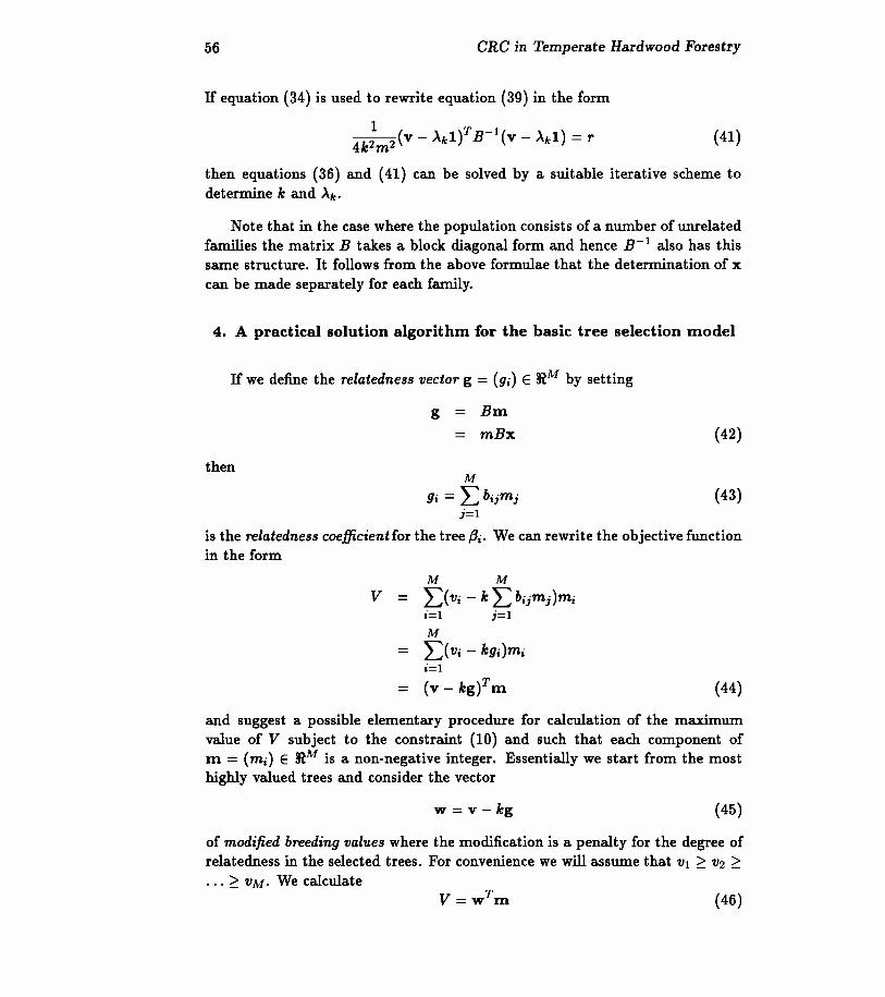
ITequation (34) is used to rewrite equation (39) in the form
4k;m2(v - Akl)TB-l(V - Ak1) = r (41)
then equations (36) and (41) can be solved by a suitable iterative scheme todetermine k and Ak.
Note that in the case where the population consists of a number of unrelatedfamilies the matrix B takes a block diagonal form and hence B-1 also has thissame structure. It follows from the above formulae that the determination of xcan be made separately for each family.
4. A practical solution algorithm for the basic tree selection model
ITwe define the relatedness vector g = (gi) E lJlM by setting
g Bm
mBx (42)
thenM
gi = Ebijmjj=1
is the relatedness coefficient for the tree {3i. We can rewrite the objective functionin the form
(43)
M MV E(Vi - k E bijmj)mi
i=l j=l
M
E(Vi - kgi)mii=1
(v-kgfm (44)
and suggest a possible elementary procedure for calculation of the maximumvalue of V subject to the constraint (10) and such that each component ofm = (mi) E lJlM is a non-negative integer. Essentially we start from the mosthighly valued trees and consider the vector
W = v - kg (45)
of modified breeding values where the modification is a penalty for the degree ofrelatedness in the selected trees. For convenience we will assume that VI ~ V2 ~
••• ~ VM. We calculate(46)
Tree breeding programs 57
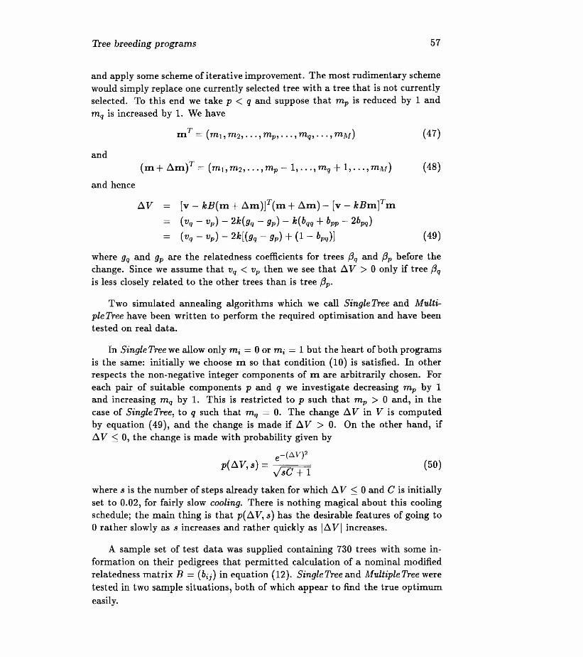
and apply some scheme of iterative improvement. The most rudimentary schemewould simply replace one currently selected tree with a tree that is not currentlyselected. To this end we take p < q and suppose that mp is reduced by 1 andmq is increased by 1. We have
(47)
and
and hence
AV [v - kB(m + Am)]T(m + Am) - [v - kBmf m(vq - vp) - 2k(gq - gp) - k(bqq + bpp - 2bpq)(vq - vp) - 2k[(gq - gp) + (1- bpq)] (49)
where gq and gp are the relatedness coefficients for trees (Jq and (Jp before thechange. Since we assume that Vq < vp then we see that AV > 0 only if tree (Jqis less closely related to the other trees than is tree (Jp.
Two simulated annealing algorithms which we call Single Tree and Multi-pleTree have been written to perform the required optimisation and have beentested on real data.
In Single Tree we allow only mi = 0 or mj = 1 but the heart of both programsis the same: initially we choose m so that condition (10) is satisfied. In otherrespects the non-negative integer components of m are arbitrarily chosen. Foreach pair of suitable components p and q we investigate decreasing mp by 1and increasing mq by 1. This is restricted to p such that mp > 0 and, in thecase of Single Tree, to q such that mq = O. The change AV in V is computedby equation (49), and the change is made if AV > O. On the other hand, ifAV :S 0, the change is made with probability given by
e-(.6.V)2
p( A V, s) = ~v't=;;;=='7sC + 1
(50)
where s is the number of steps already taken for which AV :S 0 and C is initiallyset to 0.02, for fairly slow cooling. There is nothing magical about this coolingschedule; the main thing is that p( AV,s) has the desirable features of going too rather slowly as s increases and rather quickly as IAV I increases.
A sample set of test data was supplied containing 730 trees with some in-formation on their pedigrees that permitted calculation of a nominal modifiedrelatedness matrix B = (bij) in equation (12). Single Tree and Multiple Tree weretested in two sample situations, both of which appear to find the true optimumeasily.

58 CRC in Temperate Hardwood Forestry
Single Tree was used with m = 20 and M = 730, and with k = 0.1. Startingwith two permutations of the input data, firstly unsorted and secondly sorted byVi > Vi+! Single Tree gave the same solution after only about 200,000 iterations,taking less than a minute and with no further improvement after an overnightrun.
In MultipleTree we allow mi to take any non-negative integer values. Thisprogram was tested with m = 60 and M = 730 and a range of k values from 0.01to 0.2 and seemed to give consistent results. Later tests with different coolingfunctions showed that choosing C ~ 10 gives the best results for k up to about0.1. More extensive testing should be done to check the most appropriate valuesfor C. Different cooling schedules all seemed to give the same apparently optimalsolutions after a few hundred thousand iterations and these solutions could notbe improved upon even if millions of iterations were tried.
In summary, the fact that MultipleTree gives the same solution when runwith different cooling schedules suggests that for these problems the simulatedannealing method is actually finding the true maximum of the objective function,and in a very short time. The time was less than a minute for the values of k, Mand m in the test examples mentioned above. This is to be expected when thestate space is asymmetric. In this regard the region of the space containing thetrees with the highest breeding values, where the optimum would be expected tolie, acts in an attractive manner. For the same reason, one would expect geneticalgorithms also to perform well.
Further evidence that the true maximum is being found by simulated anneal-ing was obtained when the Single Tree problem was reformulated as an integerlinear programming problem. Since the linear programming algorithm uses ap-proximately M2/2 variables it was necessary to make the problem size moremanagable by restricting our attention to the top 100 trees, ranked by Vi. Thiswas regarded as a fairly safe restriction since with m = 20, all trees used in thesolution found by Single Tree were ranked in the top 80 trees. After several hours,a standard package confirmed the solution found by Single Tree. The Multiple-Tree problem is much harder to write as an integer linear programming problembecause each quadratic term bijmjmj in equation (13) can take on more thantwo possible values.
5. Existence of a solution in non-negative integers for the basic treeselection model in the case of a population of unrelated clones.
It is common practice in seed orchards to plant equal numbers of essentiallyunrelated clones. We ask whether the expected breeding value could be increased

Tree breeding programs 59
by using more of the superior clones. In this case we have
(51)
for j i= i and the objective function defined in equation (11) reduces to
M
V = L)vjmj - km;];=1
(52)
and is a special case of the more general form
M
V = L[v;mj - f(m;)];=1
(53)
which must be maximised subject to condition (10) and subject to the restrictionthat each component of In = (m;) E lRM is a non-negative integer. Once againwe assume that VI 2 V2 2 ... 2 VM. If In E !RM is a feasible selection and ifmp < mq for some p < q then we can see that the new selection with mp andmq interchanged will change V by an amount
(54)
If vp > Vq then ~ V > 0 and the new selection is better. Since there are onlya finite number of alternatives it follows from this reasoning that an optimalsolution exists and that the optimal solution will satisfy
(55)
This problem can be solved very effectively using dynamic programming withthe total number of iterations required of the order of M3• Although it is notnecessary to argue that condition (55) holds it is nevertheless true that the useof this condition makes the solution scheme more efficient. We formulate theproblem in the following way. Let P(j, t) denote the problem of selecting thenumbers
(56)
withM
L m;=t;=j+l
(57)
so thatM
Vj = L [Vim; - f(m;)]i=j+I
(58)
is maximised. If we write
V(j, t) = max{Yj I mj+I 2 .. ·2 mM 2 0 and mj+l + ... + mM = t} (59)

60 GRG in Temperate Hardwood Forestry
then it is clear that
The dynamic programming solution uses equation (60) to solve the problemsP(M, t), P(M - 1, t), ... in sequence for all t = 0,1, ... , m.
6. The entropy model
The genetic diversity of the current population Pt can be measured by theentropy which is defined by
N
H(Pt) = (-1) LVj(Pt)logvj(Pt)j=l
(61)
where v(Pt) is the genetic measure defined in equation (6). For the originalpopulation we have
1vj{Po) = N
for each i = 1,2, ... , N and hence
(62)
H(Po) = log N. (63)
It is clear that(64)
and although it is not true to say that the entropy of the population decreaseswith time we observe that if
(65)
for i = i.,h,....i« then
H(Pa) :S log(N - n) (66)
for all s 2: t. These ideas are also illustrated by the simple example in Section 8.
As before we suppose the current population P = Pt is denoted by 131,... , 13Mand that we use mi clones of the individual f3i for each i = 1,2, ... , M. Wesuppose that the genetic content of f3i is denoted by
V(f3i) = (67)

Tree breeding programs 61
and we note thatNL lIij = 1.
j=l
The entropy of the effective population is given by
N
H = (-1) L IIj loglljj=l
(68)
(69)
whereM
IIj = L "ijZi·i=l
(70)
It is convenient to begin by solving an unconstrained problem. We show thatthe entropy of the effective population is maximised by choosing Zl, Z2, ... , ZM
in such a way that1
"1 = "2 = ... = IIN = N·
Because of the conditions (10) and (68) we have
(71)
H H(Zb Z2,···, ZM-1)N
(-1) L IIj log IIjj=l
(72)
whereM-I
IIj = L (lIij - IIMj)Zi+ "Mji=l
(73)
for each j = 1, 2, ... , N - 1 and where
N-1
IIN = 1- E IIj.j=l
(74)
Now we calculate
(75)
and solve the equations
BH = 0 (76)BZi
for each i = 1,2, ... , M - 1. It is clear that this gives M - 1 linear equations inthe N - 1unknowns
(VI) (VN-I)log IIN , ••. ,log ~ . (77)

62 CRC in Temperate Hardwood Forestry
ITM ::::N and the rank of this set is equal to N - 1 then the unique solution isgiven by
log (:~) = 0 (78)
for each j = 1,2, ... ,N - 1. Thus, in this generic case, we can see that H ismaximised when "1 = "2 = ... = "N·
Strictly speaking we should solve the above problem subject to the addi-tional constraint x ::::0 but because the solution is not conditional on theserestrictions we can formally omit them. This is an important point in relationto our subsequent arguments with the real constrained selection problem.
We now wish to maximise the entropy H subject to the constraints V ::::Vo,where Vo is the minimum allowed total breeding value, x ::::0 and 1T X = 1. Wedefine a Lagrangean function
(79)
where "-E lRand .\ E RM are Lagrange multipliers with "- ::::0, .\ ::::0 and applythe Kuhn-Tucker equations
a'J-l = 0aZi
for each i = 1,2, ... , M -1 and the complementary slackness conditions to obtainthe necessary conditions
(80)
for each i= 1,2, ... ,M -1 and
(81)
Therefore we again have M - 1 linear equations in the N - 1 unknowns
log (:~ ) , ... , log (":~I)but since the equations are now non-homogeneous we can no longer expect anunconstrained solution. In fact, if we assume that .Ai = 0 for N different valuesof i we can obtain a solution for the corresponding Zi in which each of these Zi
is strictly positive. All other Zi are set to zero and the corresponding .Ai and "-are determined from the remaining equations.
(82)

Tree breeding programs 63
The important insight is that we expect only N of the variables :1:1, •.• , :I:M
will be non-zero.
More information about this technique can be obtained from a technicalreport by Howlett et al. (1996).
7. The enhanced tree selection model
In the previous models an implicit assumption about breeding values is thatthe breeding value of the offspring of a particular mating is the average of thebreeding values of the two parents and hence we have assumed that
(83)
This is tantamount to saying that the best parents will produce the best offspringand on average this is observed to be true. Although this is a useful assumptionin models with an unbiassed selection of the next generation of breeding trees theassumption is not appropriate when we choose only the best progeny from eachcross and when we wish to make projections about the consequent improvementin breeding values over several generations.
It is clear that the genetic structure of the offspring is not determineduniquely for each mating pair. Each individual in the population carries a fixednumber of chromosomes and the offspring of a particular cross receives thesechromosomes from one or other of the parents. The allocation of the chromo-somes is essentially a random process. If there are k different chromosomes thenthere are 2k different genetic combinations that could be obtained. It is there-fore more reasonable to regard the breeding value Vij for the progeny f3i X f3jas a random variable. Since the breeding value is determined by a large num-ber of independent characteristics we could assume that Vij is a normal randomvariable with probability density function given by
N[JLij, O"i/] ( v)
1 [ 1 (v - JLij) 2]----,= exp - - .O"ij...J2i 2 O"ij
(84)=
Appropriate values for the parameters should really be determined by experi-ment. On the other hand we could assume that the breeding value Vi of eachindividual f3i is a random variable and that the random variable Vij is deter-mined from the random variables Vi and Vj by a simple formula. Indeed, if weassume that
1 1v... - -V; + -v·IJ - 2 I 2 J (85)

64 CRC in Temperate Hardwood Forestry
then we could argue that
J.Lij E[Vij]1 1
E[-V.· + -V]2 I 2}1 1"2 J.Li + "2 J.Lj (86)
and
U··2I} E[(Vij - J.Lij)2]
E[l(Vi - J.Li)2 + l(Vj - J.Lj)2 + ~(Vi - J.L;)(Vj - J.Lj)]
1 2 1 2 1:tu; + :tUj + "2a;jU;Uj (87)
where A = (aij) E !RMxM is the relatedness matrix and where we have assumedfor the sake of argument that
(88)
If nij is the number of progeny produced from f3i X f3j and if Wij is the minimumacceptable breeding value from this cross then the expected number of progenyselected for the next breeding population will be given by
(89)
and the associated expected mean breeding value will be
Vij = !.w~Vlij(v)dv.)
Uij [1 (Wij - J.Lij) 2]--exp --.y'27r 2 Uij (90)
We need to select nij and Wij for i, i = 1,2, ... , M and i ~ j such that wemaximise the overall expected breeding value
(91)
subject to the equality constraint
L mij = ml~i~j~M
(92)
Tree breeding programs 65
and the inequality constraint
(93)
where m is the total number of progeny we wish to select, Ps is the populationof selected progeny and r is some fixed number with 0 :S r < N. This problemcan be formulated as a standard finite dimensional constrained optimisationproblem.
The main importance of this model is that it is not only a model for makinga good selection for the next generation of breeding stock but is also a modelthat allows us to estimate the expected improvement in the breeding populationfrom one generation to the next. This could be useful for forward projectionsconcerned with the economic viability of the breeding operation.
8. A simple example
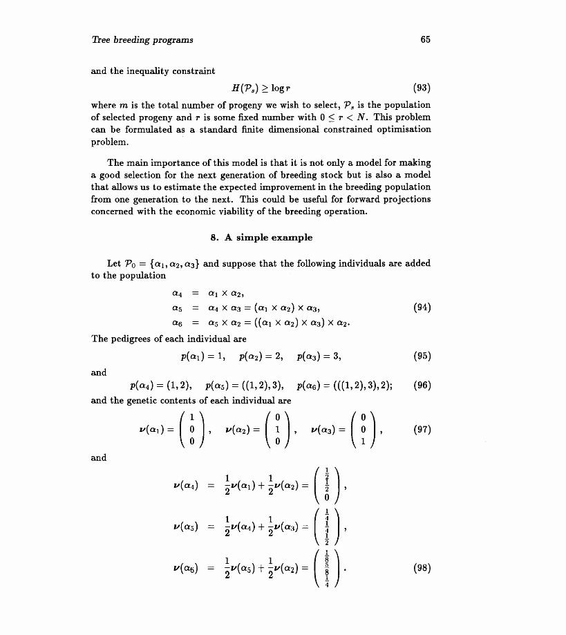
Let Po = {a1' a2, a3} and suppose that the following individuals are addedto the population
a4 al X a2,
a5 a4 X a3 = (a1 X (2) X a3, (94)a6 a5 X a2 = ((al X (2) X (3) X a2.
The pedigrees of each individual are
p(at} = 1, p(a2) = 2, p(a3) = 3, (95)and
p(a4) = (1,2), p(a5) = ((1,2),3), p(a6) = (((1,2),3),2); (96)and the genetic contents of each individual are
v(ad = 0), v(a,) = ( n, v(a3) = 0)' (97)
and
v(a4)1 1 (n'2"v(at} + 2"v(a2) =
( 1 ),1 1 4"v(a5) 2"v( (4) + 2"v( (3) = 1
4"12"
( 1 ).1 1 8v(a6} 2v(a5) + 2v(a2) = 5 (98)8
14"
66 CRC in Temperate Hardwood Forestry
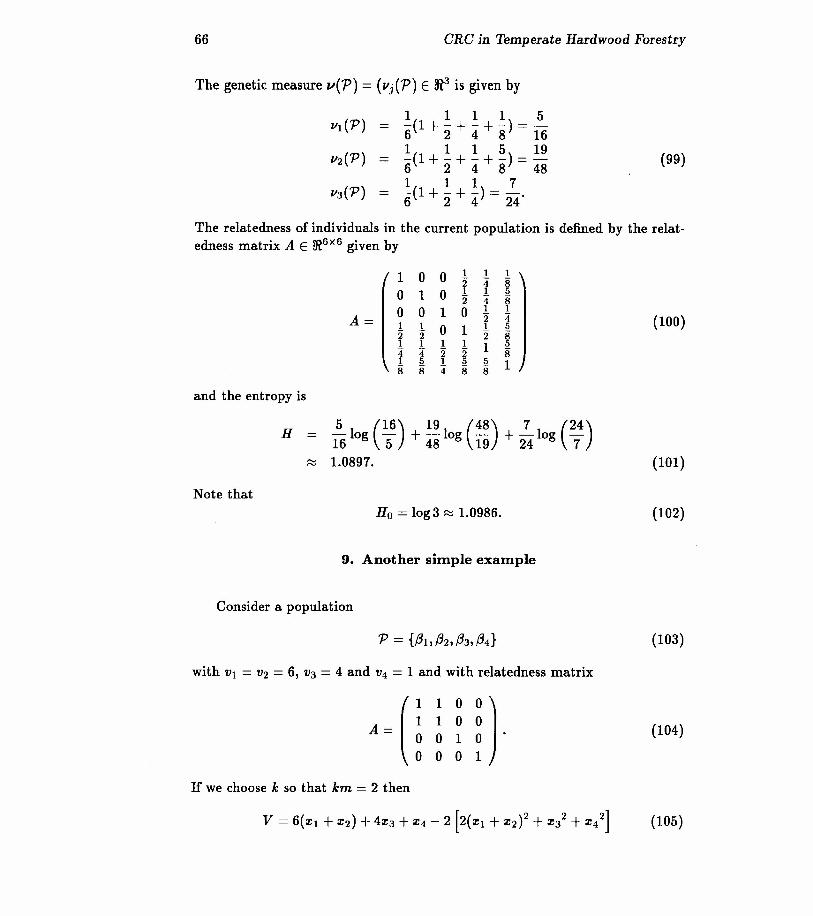
The genetic measure v(P) = (Vj(P) E 313 is given by
1 1 1 1 56(1 + 2 + 4 + 8) = 161 1 1 5 196(1+2+4+8)=481 1 1 76(1 + 2 + 4) = 24·
(99)
The relatedness of individuals in the current population is defined by the relat-edness matrix A E !R6X6 given by
1 0 0 I I I"2 4" 8
0 1 0 I I 5"2 4" 8
0 0 1 0 I I
A= "2 4"I I 0 1 I 5"2 "2 "2 8I I I I 1 54" 4" "2 "2 8I 5 I 5 5 18 8 4" 8 8
(100)
and the entropy is
H ~log (16) + 19 log (48) + l..-log (24)16 5 48 19 24 7
~ 1.0897. (101)
Note thatHo = log 3 ~ 1.0986. (102)
9. Another simple example
Consider a population
(103)
with VI = V2 = 6, V3 = 4 and V4 = 1 and with relatedness matrix
(104)
If we choose k so that km = 2 then
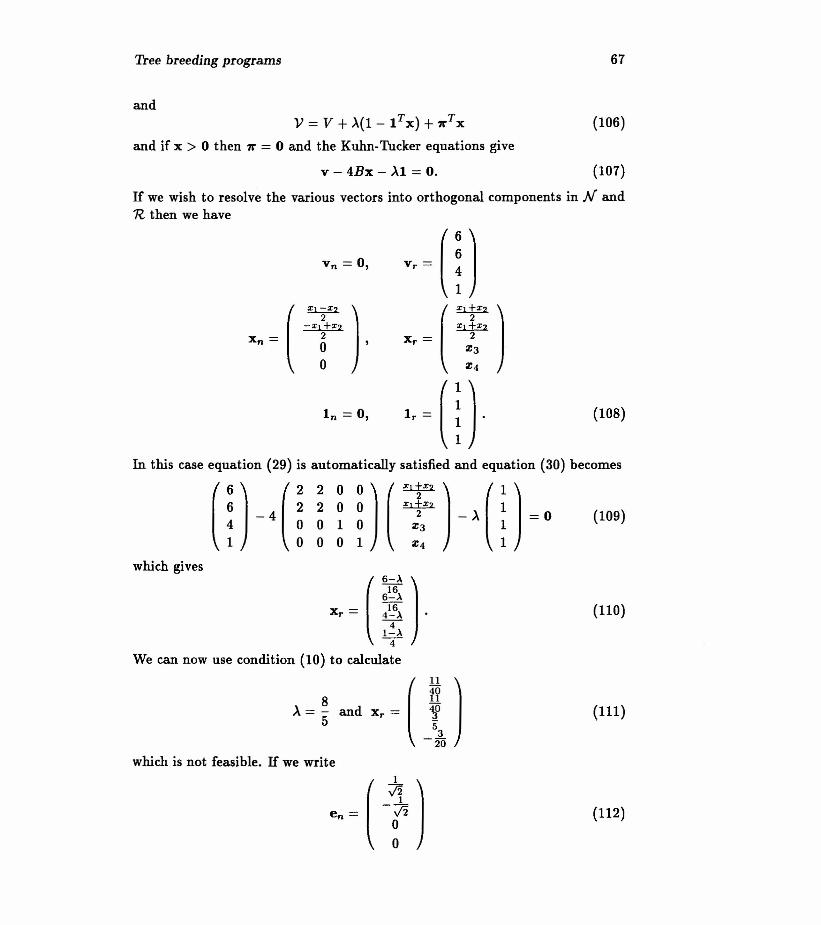
Tree breeding programs 67
andv = V + A(l - IT x) + 7rT x
and if x> 0 then 7r = 0 and the Kuhn-Tucker equations give
v - 4Bx - Al = o.
(106)
(107)
ITwe wish to resolve the various vectors into orthogonal components in.N andR then we have
Vn = 0, Vr = (n(= ) (~)_ -X!~+X2 ~
Xn - 0 ' x, = 2Z3
0 Z4
In = 0, 1, = (i)- (108)
In this case equation (29) is automatically satisfied and equation (30) becomes
which gives
x, = ( :~~ ) .1-~-4-
We can now use condition (10) to calculate
l=~=dx'=(JJ
(110)
(111)
which is not feasible. ITwe write
(112)

68 CRC in Temperate Hardwood Forestry
then we find that the solution set
S = [xjx = x, + ()en for () E !R} (113)does not intersect the feasible set F. On the other hand if we assume that :l:4 = 0and delete :l:4 from the problem then equation (30) becomes
(6) (2 2 O)(~) (1): - 4 ~ ~ ~ XI}:2 - A ~ = 0
(114)which gives
(
6~6A )6-Ax; = 16"4-A-4-
and we can use condition (10) to calculate
A = 2 and x, = ( 1 )t
(115)
(116)which is feasible. If we write
en = ( -}, ) (117)
the entire solution set is
(118)and the set of feasible solutions is given by
{ I () E [- V242, V242]}S n F = x x = x, + ()en for all (119)
with V(x) = Vmax = ~ for all x E S n F.
10. Discussion
In summary we simply observe that The basic tree selection model has beenfully analysed and tested and appears to offer an effective selection procedurefor the next generation of breeding stock. The entropy model although not fullydeveloped offers an alternative procedure that we believe would simply changethe emphasis of the selection rather than the nature. The enhanced tree selectionmodel is a proposal that could be used as a basis for a more comprehensive schemethat is concerned with longer term analysis over several generations.

Tree breeding programs 69
Acknow ledgements
The moderators, Colin Thompson and Phil Rowlett, would like to thank theindustry representatives, Nuno Borrahlo, Mike Powell, Richard Kerr, and PeterGore, and the other team members, Nick Wormald, Bill Whiten, Jerzy Filar,Genevieve Mortiss, Ernie Chow, Jemery Day, Natashia Boland, Pierre Prado,David Peel, Matthew York and Peter Watson for their special inspirations andexcellent co-operation. We were particularly grateful for the willingness of teammembers to undertake the various specific tasks that were handed out from timeto time. We would also like to thank Tim Thwaites for compiling the executivesummary.
References
J.R. Brisbane and J.P. Gibson, "Balancing selection response and rate of in-breeding by including genetic relationships in selection decisions" Theoryand Application of Genetics 91 (1995),421-431.
P.G. Rowlett, J.A. Filar, C.J. Thompson and G. Mortiss, "An entropy modelfor selection and mating decisions in tree breeding programs", School ofMathematics Report, University of South Australia (in preparation).
G.B. Jansen and J.W. Wilton, "Selecting mating pairs with linear programmingtechniques", Journal of Dairy Science 68 (1985), 1302-1305.
T.R.E. Meuwissen and J.A. Woolliams, "Response versus risk in various breed-ing schemes", Proceedings 5th. World Conference of Genetics applied toLivestock Production, University of Guelph, Canada (1994), 236-243.
M. Sedgley and A.R. Griffin, Sexual Reproduction of Tree Crops (AcademicPress, 1989).