Embed Size (px)
Citation preview

Geophys. J. Int. (2003) 154, 483–498
Modelling of seismic waves in heterogeneous media using awavelet-based method: application to fault and subduction zones
Tae-Kyung Hong and B. L. N. KennettResearch School of Earth Sciences, Institute of Advanced Studies, The Australian National University, Canberra, ACT 0200, Australia.E-mails: [email protected]; [email protected]
Accepted 2003 March 5. Received 2003 March 3; in original form 2002 November 18.
S U M M A R YThe wavelet approach to numerical simulation of elastic wave propagation is applied to modelswith localized heterogeneity, with significant contrasts with their surroundings. We considerzones with both lowered wave speed such as a fault gouge zone and elevated wave speeds suchas in a subduction zone. In each of these situations the source lies within the heterogeneity.The representation of the source region has therefore been adapted to work directly in aheterogeneous environment, rather than using a locally homogeneous zone around the source.This extension also allows the wavelet method to be used with a wider variety of sources,e.g. propagating sources. For the fault zone we consider both point and propagating sourcesthrough a moment tensor representation and reveal significant trapped waves along the gougezone as well as permanent displacements. For subduction zones a variety of effects are produceddepending on the depth and position of the source relative to the subducting slab. A varietyof secondary waves, such as reflected and interface waves, can be produced on wave trains atregional distances and tend to be more important for greater source depths.
Key words: elastic-wave theory, fault, heterogeneous media, numerical techniques, subduc-tion zone, wavelets.
1 I N T RO D U C T I O N
Tectonic regions are associated with complex and faulted structures,which can bring material with considerable contrast in propertiesinto close proximity. Earthquakes are initiated in regions of consid-erable heterogeneity, which needs to be taken into account in thedescription of the generation of seismic waves by the source. Smalldistortions in the wavefield associated with systematic structure canlead to substantial differences on further propagation (e.g. Li &Vidale 1996).
It is therefore necessary to develop techniques that can considersources in a heterogeneous environment and that do not dependon the commonly used assumption of local homogeneity near thesource (e.g. Alterman & Karal 1968; Kelly et al. 1976; Levander1988). In many circumstances such an approximation can work wellwhen waves propagate from a simple into a more complex zone (e.g.Yomogida & Etgen 1993), but may be misleading where the sourceregion itself is complex.
Two representative regions in the Earth where tectonic processesdevelop strongly heterogeneous structures in which earthquakes ini-tiate are fault and subduction zones. Many different styles of numeri-cal techniques have been used to simulate the propagation of seismicwaves in such regions. Finite-difference methods have been used ininvestigating trapped waves in fault zones (Li & Vidale 1996; Igelet al. 2002) and guided waves in a subduction zone with an accre-tionary prism (Shapiro et al. 2000). To study waveform and ampli-
tude variations associated with subduction zones, Vidale (1987) ap-plied a coupled finite-difference and Kirchhoff method, Furumura &Kennett (1998) implemented a pseudospectral method, and Cormier(1989) and Sekiguchi (1992) used Gaussian-beam methods.
Classical finite-difference techniques (e.g. Alterman & Karal1968) generally need more gridpoints per wavelength than othermethods implementing a high-accuracy differentiation scheme (e.g.the pseudospectral method). Since a large region needs to be con-sidered for subduction zone modelling memory requirements arehigh. If strong heterogeneity needs to be modelled, numerical disper-sion is likely (Hong & Kennett 2003). Higher-order finite-differencetechniques (Igel et al. 1995; Falk et al. 1998) cure most of the limi-tations of classical finite-difference methods but require the sourcetime functions to be smooth enough to be differentiated many times.This requirement makes it difficult to handle dislocation sources forwhich the displacement time functions are both complicated andmay well not be differentiable.
The Gaussian-beam method is attractive because of its low com-putational cost for simple situations because it is built on the frame-work of ray theory, with the superposition of all Gaussian beamspassing through the neighbourhood of a point. However, in zonesof high heterogeneity the ray tracing itself becomes a dauntingtask. Furthermore, it is difficult to include all necessary secondaryphases which may affect the waveforms, such as interface wavesalong a zone of contrast such as the boundary of a subductingslab.
C© 2003 RAS 483
484 T.-K. Hong and B. L. N. Kennett
Although a pseudospectral method (or Fourier method, Kosloffet al. 1984) can implement high-accuracy differentiation, thetraction-free condition on a free surface is difficult to implement ef-fectively. In the Chebyshev spectral method (Kosloff et al. 1990) thetraction-free condition is satisfied using 1-D analysis at the bound-ary, but this method also suffers from a non-uniform spatial gridspacing in the vertical direction imposed from the character of theChebyshev polynomials.
Recently, a wavelet-based method (WBM) has been introducedfor modelling of elastic wave propagation (Hong & Kennett2002a,b). Because the representation of differential operators iscarried out to high accuracy, the WBM approach is very ef-fective for describing propagation through highly heterogeneousrandom media, retaining both accuracy and stability (Hong &Kennett 2002c). In this paper we consider the extension of the WBMto a general source representation (such as dislocation sources) em-bedded in heterogeneous zones. The treatment of heterogeneity isbased on splitting the second-order differential operators in the zonearound the source into two parts, so that a simple first-order operatoris all that is left at the source location itself.
The extended WBM scheme is applied to two representative prob-lems with heterogeneous source regions: fault and subduction zones.Fault zones are composed of physically perturbed materials createdduring prior rupturing processes, and resultantly behave as low-velocity structures. In contrast, a subduction zone has a dynami-cally subducting cool slab that displays a high-velocity anomaly tosurrounding media.
In the application to fault-zone problems, we probe the effectsof trapped waves in the low-velocity fault zone and the permanentdisplacements around sources. We include dislocation sources (in-cluding a propagating rupture) in the fault zone and are able toinclude an arbitrarily complex time history of slip to handle thecomplexities of real events.
In modelling for subduction zones, we investigate waveform andamplitude variation of SH waves propagating through a subductingslab. The size of the subduction zone means that we need to takeaccount of the sphericity of the Earth and we have to make the ap-proximation of working in a cylindrical coordinate system for SHwaves. Previous studies (e.g. Sekiguchi 1992) on waveform varia-tion in subduction zones did not pay attention to effects of interfacewaves and post-critically reflected waves sufficiently in regional dis-tances, we investigate those effects by varying the relative positionof the source and the slab boundaries. In particular, since earth-quakes are, in general, close to the boundaries of the subductingslabs (e.g. Pankow & Lay 2002), there are considerable possibilitiesfor the development of interface waves that can travel considerabledistances along the slab.
2 A WAV E L E T - B A S E D M E T H O D F O RE L A S T I C WAV E M O D E L L I N G
In this section, we briefly introduce the wavelet-based method whichis described more fully in Hong & Kennett (2002a,b).
The P–SV elastic wave equation system in 2-D including bodyforce terms ( f x, f z) and absorbing boundary conditions via attenu-ation factors (Qx, Qz) is given by
∂2ux
∂t2= −2Qx
∂ux
∂t+ 1
ρ
(∂σxx
∂x+ ∂σxz
∂z+ fx
),
∂2uz
∂t2= −2Qz
∂uz
∂t+ 1
ρ
(∂σxz
∂x+ ∂σzz
∂z+ fz
), (1)
where (ux, uz) is the displacement vector and (σ xx, σ xz, σ zz) arecomponents of the stress tensor:
σxx = (λ + 2µ)∂ux
∂x+ λ
∂uz
∂z, σzz = λ
∂ux
∂x+ (λ + 2µ)
∂uz
∂z,
σxz = µ
(∂ux
∂z+ ∂uz
∂x
), (2)
and λ(x , z) and µ(x , z) are the Lame coefficients. The attenuationfactors Qj( j = x , z) control the dissipation rate of waves at theabsorbing boundaries.
By introducing linear operators (Li j , i , j = x , z) for spatial differ-ential operators and recasting the governing equation system (1) ina displacement–velocity formulation, we obtain a set of first-orderpartial differential equations (PDEs) in time:
∂ux
∂t= vx ,
∂vx
∂t= −2Qxvx + Lxx ux + Lxzuz + fx
ρ,
∂uz
∂t= vz,
∂vz
∂t= −2Qzvz + Lzx ux + Lzzuz + fz
ρ, (3)
where (vx, vz) is the velocity vector and the operators Li j are givenby
Lxx = 1
ρ
∂
∂x
[(λ + 2µ)
∂
∂x
]+ 1
ρ
∂
∂z
(µ
∂
∂z
),
Lxz = 1
ρ
∂
∂x
(λ
∂
∂z
)+ 1
ρ
∂
∂z
(µ
∂
∂x
),
Lzx = 1
ρ
∂
∂x
(µ
∂
∂z
)+ 1
ρ
∂
∂z
(λ
∂
∂x
),
Lzz = 1
ρ
∂
∂x
(µ
∂
∂x
)+ 1
ρ
∂
∂z
[(λ + 2µ)
∂
∂z
]. (4)
The equation system (3) can be written as a form of first-orderdifferential equation with a vector unknown U:
∂t U = LU + N, (5)
where U is (ux, vx, uz, vz)t and the operator matrix L is given by
L =
0 I 0 0
Lxx −2Qx Lxz 0
0 0 0 I
Lzx 0 Lzz −2Qz
. (6)
N is composed of the body forces (0, f x/ρ, 0, f z/ρ)t. When ad-ditional boundary conditions are considered, such as traction-freeconditions on a free surface or inside a medium (e.g. a medium witha cavity), these conditions can be expressed via equivalent forcesusing the stress values on the boundaries, added to the body forcecomponents in N.
Spatial differentiations of displacement or velocity fields are con-ducted on wavelet spaces by projecting the differential operators andvector fields using a wavelet transform. The differentiated fields arerecovered by recombining all the wavelet space contributions us-ing an inverse wavelet transform. For more details, refer to Beylkin(1992) and Hong & Kennett (2002a,b).
With a semi-group approach (e.g. Beylkin & Keiser 1997), thediscrete time solution of eq. (5) is given by
Un+1 = Un + δtLUn + δt2
2L2Un + · · · + δtm
m!LmUn
+ δtNn + δt2
2LNn + δt3
6L2Nn + · · · + δtm+1
(m + 1)!LmNn, (7)
C© 2003 RAS, GJI, 154, 483–498
A wavelet-based method for heterogeneous media 485
where δ t is a discrete time step, Un is the displacement–velocityvector at discrete time tn, N n is a vector of forcing terms and mcontrols the truncation order in the discrete time solution.
As we can see from eq. (7), this scheme needs multiple spa-tial differentiations on a delta function for a point force (e.g. LNn), and numerical dispersion will occur if the matrix operator L
is applied directly. This problem can be avoided if the source re-gions are assumed to be locally homogeneous, and linear opera-tors are formulated in simplified forms where multiple first-orderdifferentiations are replaced by a second-order differentiation (e.g.∂ x (a ∂ x u) → a ∂2
x u). So, the linear operators (Lsi j ) in the source
region are represented by
Lsxx = (λs + 2µs)
ρ
∂2
∂x2+ µs
ρ
∂2
∂z2, Ls
xz = Lszx = (λs + µs)
ρ
∂2
∂x∂z,
Lszz = µs
ρ
∂2
∂x2+ (λs + 2µs)
ρ
∂2
∂z2, (8)
where λs and µs are values of the Lame coefficients at the sourceposition and Ls
i j are the components of the matrix operator (Ls) inthe source region. By applying this source-region scheme with Ls
while the source is active, the WBM sustains numerical stability.However, when a source is initiated in a heterogeneous region this
approach is no longer valid and needs to be modified as discussedin the next section.
3 M O D I F I E D T E C H N I Q U E
3.1 Theory
We modify the source representation by using a linear combinationof operators to cope with heterogeneity, whilst retaining numericalstability. We require that the operators both inside and outside thesource zone should be equivalent to the linear operators Li j in eq.(4) for a general medium. We extract the Ls
i j contribution in thesource region, and write the new form of the linear operators Lr
i j as
Lrxz = Lxz, Lr
xx =Lxx , z > zs + l, z < zs − l,
Lsxx + Ld
xx , zs − l ≤ z ≤ zs + l,
Lrzx = Lzx , Lr
zz =Lzz, x > xs + l, x < xs − l,
Lszz + Ld
zz, xs − l ≤ x ≤ xs + l,
(9)
where (x s, zs) is the source position and l defines the size of theimmediate source zone. The additional operators Ld
j j ( j = x , z) in aheterogeneous source zone take the form
Ldxx = 1
ρ
∂
∂x
[(λ + 2µ)
∂
∂x
]+ 1
ρ
∂
∂z
(µ
∂
∂z
),
Ldzz = 1
ρ
∂
∂x
(µ
∂
∂x
)+ 1
ρ
∂
∂z
[(λ + 2µ)
∂
∂z
], (10)
where λ(x , z) = λ(x , z) − λs and µ(x , z) = µ(x , z) − µs.It can be readily proved that Ls
j j + Ldj j is mathematically equiv-
alent to L j j . Also, note that the terms Li j (i = j) do not need tobe recast in the new form since only multiple differentiations in thesame direction (e.g. ∂ x∂ x or ∂ z∂ z) develop numerical instability andthey are not included in these operators. Therefore, the original formof Li j can be implemented directly when i = j .
In addition, we can find that only the linear operators Lsi j are
needed at the source position since the Lame coefficient differenceterms (λ, µ) vanish at this point. So, with this modified linearoperators Lr
i j , one can treat any variation in the properties of sourceregions without numerical dispersion.
Source
10 km
10 km
ΓRΓL
ΓB
ΓT
R1 R2 R3 R4
D1 D2 D3 D4
Ω1
Ω2
4.53 km
x
z
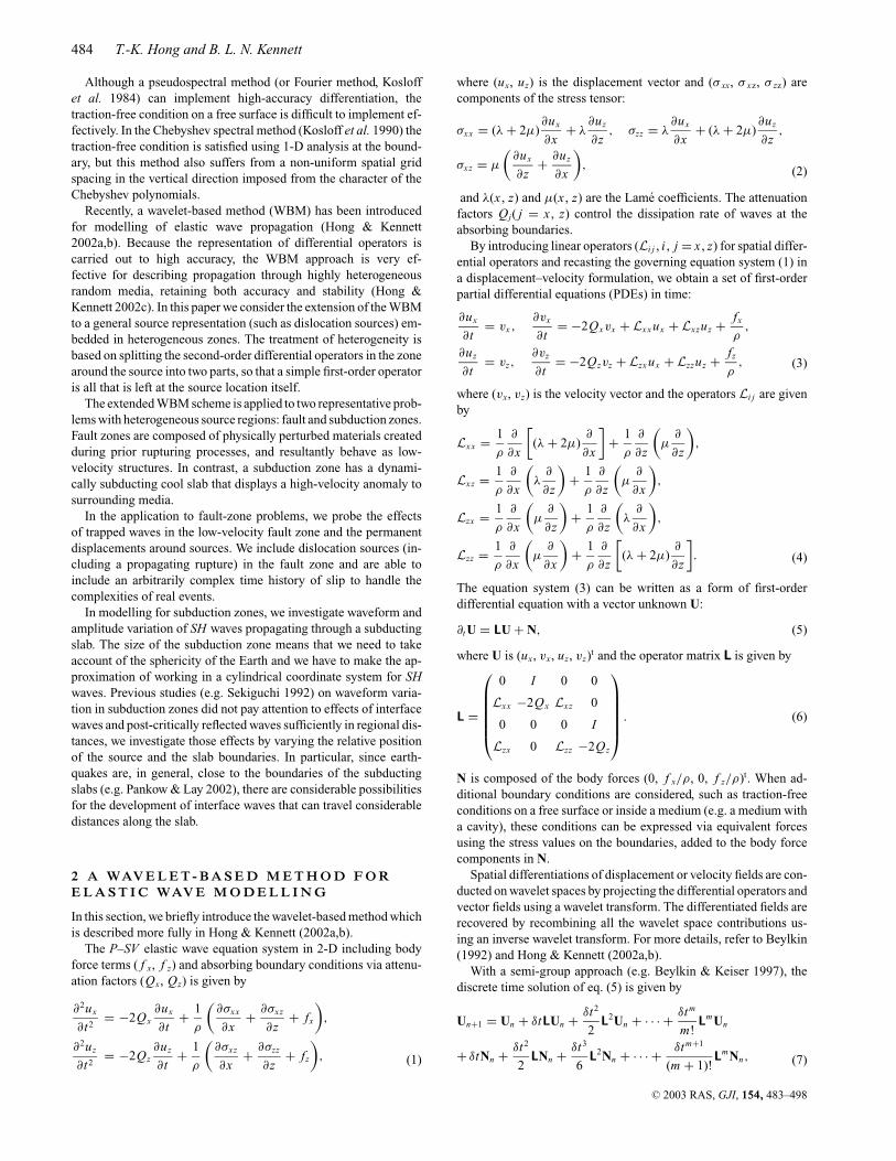
Figure 1. Representation of the two-layered medium used for the validationtest of the modified WBM. The domain is 10 ×10 km2 and a planar internalboundary is placed at a depth of z = 4.53 km. The compressional wavevelocity (α1) in the top layer (1) is 3.5 km s−1, the shear wave velocity(β1) is 2.0 km s−1, and the density (ρ1) is 2.2 Mg m−3. The velocities inthe bottom layer (2) are twice those in the top layer (i.e. α2 = 7.0 km s−1,β2 = 4.0 km s−1) and the density (ρ2) is 3.3 Mg m−3. A vertically directedpoint source is applied at (2.34 km, 2.97 km), and four artificial boundaries(T , B , R , L ) are treated by absorbing boundary conditions. In orderto record time responses, eight receivers are deployed at depths of z =3.75 km (Rj, j = 1, . . . , 4) and 6.88 km (Dj) from x = 2.5 km with aconstant spacing of 1.875 km.
3.2 Validation test
In order to test whether the modified procedure is equivalent tothe previous technique (Hong & Kennett 2002a,b), which has beenvalidated by comparison with analytical solutions and other numer-ical methods, we compare the time responses of both techniques in aheterogeneous situation. We implement several values of l and com-pare the results to determine a suitable value for accurate and stablemodelling and also to investigate whether any numerical anisotropyarises from the implementation of a combination of linear operators(see, e.g., Kaser & Igel 2001).
We consider a two-layered medium (Fig. 1) in a 10×10 km2
domain, represented by 128 × 128 gridpoints. The elastic wavevelocities in the lower layer are twice those in the upper layer andthe density ratio is a factor of 1.5. The four artificial boundaries(T , B , R , L ) are treated via absorbing boundary conditions.A vertically directed point force is applied at (2.34 km, 2.97 km)inside the upper layer and eight receivers (Rj, Dj t j = 1, . . . , 4) aredeployed with a spacing of 1.875 km starting from x = 2.5 km atdepths of z = 3.75 and 6.88 km. A Ricker wavelet with dominantfrequency 4.5 Hz is introduced as the source time function.
When direct P and S waves are incident on an internal boundary,reflected (PPr, PSr, SPr, SSr) and transmitted (PPt, PSt, SPt, SSt)waves with phase coupling, interface waves and head waves developand propagate from the boundary as indicated in Fig. 2.
We consider three different implementations of the modified ap-proach with different values of l, and compare the resulting seismo-grams with those for the previous scheme. In case A we considerusing the sum of the two operators Ls
j j and Ldj j across the whole
domain. In the other two cases we consider a more localized appli-cation of the split operator. In case B we use three grid steps for l,and in case C the extreme position where the modified technique
C© 2003 RAS, GJI, 154, 483–498

486 T.-K. Hong and B. L. N. Kennett
-10
-8
-6
-4
-2
0z
(km
)
0 2 4 6 8 10
x (km)
-10
-8
-6
-4
-2
0
z (k
m)
0 2 4 6 8 10
x (km)
t=1.5 s
X comp. Z comp.
PS
PPtPSt
PPr
PSr
SSt
Figure 2. Snapshots of elastic wave propagation in the two-layered medium of Fig. 1 at t = 1.5s. Incident P and S waves are reflected (PPr, PSr, SPr, SSr) andtransmitted (PPt, PSt, SPt, SSt) with phase coupling on the boundary.
is just the row and column of gridpoints in which the source areplaced.
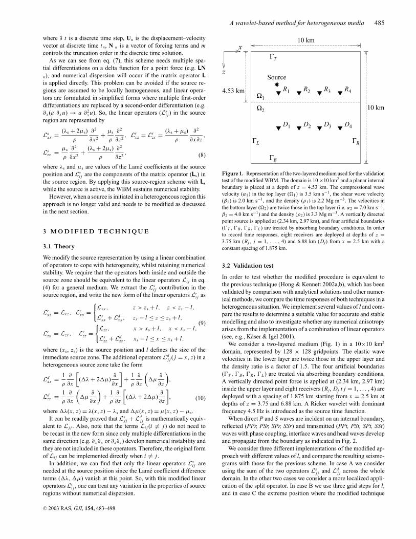
Fig. 3 displays a comparison of the numerical results for thethree cases with reference solutions calculated using the previ-ous approach. In general, the numerical results for cases A andB agree well with reference solutions for the whole wave trains ex-cept for a couple of slight misfits (indicated by the solid arrowsin Fig. 3). These effects may arise from numerical anisotropy (e.g.Kaser & Igel 2001), whereby the successive action of operatorscan have different effects depending on the order of applicationand analytically equivalent operators can have different numericalproperties.
Although case C needs much less computational effort, the qual-ity of the time response is not satisfactory. There are numericallydispersed phases arriving before the first-arrival phases and someslight misfits among the main phases (marked by broken arrows).The problem is that the operator is acting on too small a region toachieve accurate results. The quality of the time response can beensured by applying the modified technique in a ‘sufficiently broadlocalized’ area, i.e. a band of rows and columns including a sourceposition. Case B satisfies the number of gridpoints per wavelengthneeded for the WBM based on Daubechies-20 wavelets, i.e. threegridpoints (Hong & Kennett 2002a,b), and generates time responsesthat match well with the reference solutions.
Also, it is worth mentioning that the solutions, except for case A,display slight oscillations after main phases (see, a in the figure).This phenomenon is also related to numerical anisotropy, whichdevelops through the transition of numerical schemes in limited ar-eas. Here, note that the reference solutions are computed by theprevious technique in Hong & Kennett (2002a,b), which needsboth a source-region and a main-region scheme. In contrast, thecase A displays good results. However, the maximum amplitudeof the oscillations is less than 2 per cent of that of main phasesand reduces with time, and thus the oscillations do not affect wave-fields. In the following modelling, we implement the scheme forcase A.
4 M O D E L L I N G I N FAU LT Z O N E S
The implementation of a realistic fault source in numerical mod-elling has been a challenging issue, and many studies have con-fined their scope to cases using simple single-body forces (e.g.Huang et al. 1995; Igel et al. 2002). Although some SH stud-ies based on finite-difference techniques (Vidale et al. 1985; Li& Vidale 1996) have managed to incorporate dislocation sourcesby considering near-field displacement fields with approximate an-alytic representations, such dislocation modelling is still difficultfor P–SV waves. An attempt to incorporate dislocation sources in aP–SV -wave system by controlling stress values around a sourceposition has been made by Coutant et al. (1995), but the pro-posed scheme is unsatisfactory for accurate modelling. Moreover,since a real fault zone is highly heterogeneous it is desirable to beable to implement dislocation sources, including rupture in realisticmodelling.
The fault gouge zone has lowered velocities relative to its sur-roundings and so is able to support trapped waves. Such trappingphenomena have been investigated for fault zones by using 2-D (Li& Vidale 1996) and 3-D (Graves 1996) finite-difference codes orusing analytic expressions (Ben-Zion 1998). The analytic expres-sion for SH-type fault-zone trapped waves with a unit source ina uniform zone have been established by several studies (e.g. Li1988; Ben-Zion & Aki 1990; Li & Leary 1990; Li et al. 1990).They demonstrated shear waveform variations for 2-D fault zonesas a function of the parameters of the fault zone and the obser-vation pattern, e.g. fault-zone width, velocity structures, relativesource and receiver positions, and attenuation factors; they wereable to show clear development of trapped waves and head wavesas features of time responses in fault zones. The analytical ap-proach demonstrates the presence of the phenomenon but is notable to handle heterogeneity or more complex geometry. Such ef-fects can, however, be examined with numerical methods such as thehigher-order finite-difference technique (e.g. Jahnke et al. 2002),and they could treat a problem with seismic-wave initiation on a
C© 2003 RAS, GJI, 154, 483–498
A wavelet-based method for heterogeneous media 487
0 1 2 3 4 5
Time (s)
X comp.
Z comp.
R1
R2
R3
R4
R1
R2
R3
R4
a
reference solutioncase Acase Bcase C
0 1 2 3 4 5
Time (s)
X comp.
Z comp.
D1
D2
D3
D4
D1
D2
D3
D4
reference solutioncase Acase Bcase C
3.6 3.8 4 4.2
Time (s)
a reference solutioncase Acase B
Figure 3. Comparisons of time responses, for several different versions of the modified WBM with a reference solution by the previous method (Hong &Kennett 2002b). The seismograms are recorded at eight receivers (Rj, Dj, j = 1, . . . , 4) in Fig. 1. Amplified seismograms are provided for those of verticalcomponent in R4 (marked a). Case A applies the modified WBM technique to the whole domain, case B to a region three gridpoints across around the sourcepoint, and case C to a row and a column of gridpoints including a source position. Major misfits in the waveforms for case C are indicated by broken arrows,with solid arrows for other cases. The discrepancies for case C mainly arise from numerical dispersion. Records of Dj are amplified by a factor of the order of6 for display.
material boundary in a fault zone. However, the finite-differencescheme may generate artificially attenuated seismic waves in me-dia with complex strong heterogeneities (Hong & Kennett 2003)and has difficulty in treating a complex (unsmooth) source timefunction. The WBM is particularly effective in this context be-cause of its capacity to handle strong heterogeneity, and, as weshall see, is able to include a propagating rupture with a roughsource time function within the heterogeneous zone. Note thatthe WBM has been shown to preserve the energy of seismicwaves correctly even in strongly perturbed media (Hong & Kennett2003).
4.1 Implementation of dislocation sources
Dislocation sources can be implemented in the WBM through thedouble-couple force system based on a moment-tensor (M) rep-resentation, and the equivalent body force f(t) for the dislocationsources can be expressed as (e.g. Ben-Menahem & Singh 1981;Komatitsch & Tromp 2002)
f(t) = −M · ∇δ(r − rs)D(t), (11)
where D(t) is the displacement history of a particle on the fault, ris the location vector and rs is the location of the source, (x s, zs).
C© 2003 RAS, GJI, 154, 483–498
488 T.-K. Hong and B. L. N. Kennett
-10
-8
-6
-4
-2
0z
(km
)
0 2 4 6 8 10-10
-8
-6
-4
-2
0
z (k
m)
0 2 4 6 8 10
90 deg. dip-slipt=2.0 sX comp. Z comp.
N
S
P
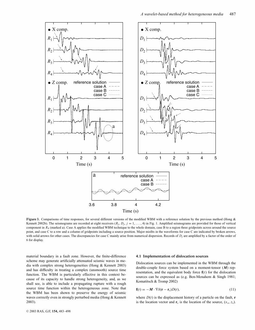
Figure 4. Snapshots of elastic wave propagation from a 90 dip-slip fault in a homogeneous medium. Both permanent displacements (N) and transientwavefields (P, S) are clearly shown.
Note that D(t) corresponds to the far-field source time function andthe area under D(t) is unity (Vidale et al. 1985; Lay & Wallace1995).
For an arbitrary fault the moment tensor can be expressed interms of strike angle (φ), dip angle (ξ ) and rake angle (η) of a faultgeometry (e.g. Lay & Wallace 1995; Kennett 2001). the strike angle(φ) is measured from the north, the dip angle (ξ ) from the horizontalplane normal to z direction and the rake angle (η) from the strikedirection on the fault plane.
We consider a thrust (90 dip-slip) fault, which is placed par-allel to the E–W direction and the corresponding moment tensorscan be computed easily for the geographic reference frame (see,e.g., Lay & Wallace 1995, p. 343; Kennett 2001, p. 72). With theassumption that there is no structural variation in the y-direction,the thrust fault source can be implemented in 2-D as a 90dip-slipfault activated on a vertical plane (x–z plane). Here, x correspondsto east and z is the downward vertical direction. The results forthis line source in 2-D can be adjusted to match the geometricalspreading in 3-D for a point source by convolving seismogramswith 1/
√t and differentiating in time (Vidale et al. 1985; Igel et al.
2002).Fig. 4 displays snapshots of elastic wave propagation in a ho-
mogeneous medium (α = 3.15 km s−1, β = 1.8 km s−1, ρ =2.2 Mg m−3) with 90dip-slip on a fault plane. Here a ramp ex-citation model where a fault slip increases linearly with time duringthe slip duration time (t r), is considered for the displacement timefunction D(t); we take 0.1 s for t r in this study. Permanent displace-ments induced by the dislocation are found in a four-lobed patternaround the source position (N in Fig. 4), and diminish with distanceas r−1. On the other hand, a transient displacement activated by prop-agating elastic waves falls off with distance as 1/
√r (Vidale et al.
1985). Therefore, in the far field, only the transient displacementsare discernible in wavefields.We are able to simulate the effect of rupture propagation by combin-ing several dislocation sources with their own source time histories,and model a simple rupture problem using a ramp source time func-tion in Section 4.3.
4.2 Modelling with a point dislocation in a fault zone
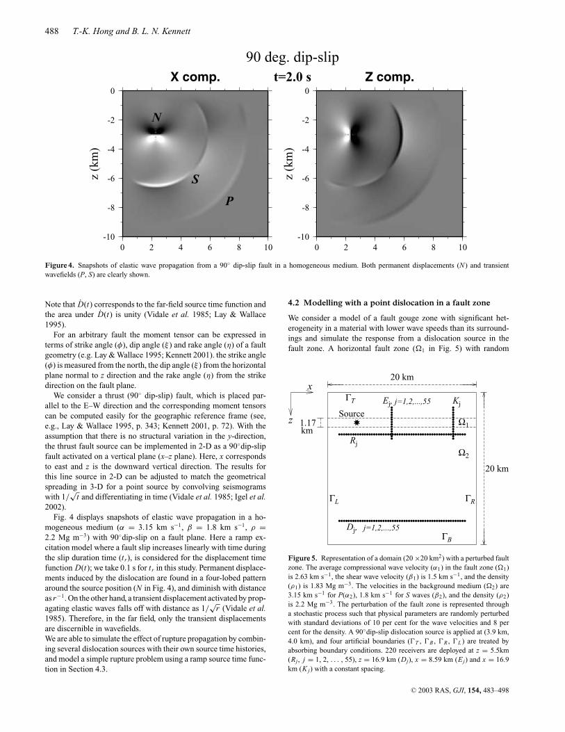
We consider a model of a fault gouge zone with significant het-erogeneity in a material with lower wave speeds than its surround-ings and simulate the response from a dislocation source in thefault zone. A horizontal fault zone (1 in Fig. 5) with random
Source
20 km
20 km
ΓRΓL
ΓB
ΓT
Rj
j=1,2,...,55
Dj, j=1,2,...,55
Ω1
Ω2
1.17km
x
z
KjEj,
Figure 5. Representation of a domain (20 ×20 km2) with a perturbed faultzone. The average compressional wave velocity (α1) in the fault zone (1)is 2.63 km s−1, the shear wave velocity (β1) is 1.5 km s−1, and the density(ρ1) is 1.83 Mg m−3. The velocities in the background medium (2) are3.15 km s−1 for P(α2), 1.8 km s−1 for S waves (β2), and the density (ρ2)is 2.2 Mg m−3. The perturbation of the fault zone is represented througha stochastic process such that physical parameters are randomly perturbedwith standard deviations of 10 per cent for the wave velocities and 8 percent for the density. A 90dip-slip dislocation source is applied at (3.9 km,4.0 km), and four artificial boundaries (T , B , R , L ) are treated byabsorbing boundary conditions. 220 receivers are deployed at z = 5.5km(Rj, j = 1, 2, . . . , 55), z = 16.9 km (Dj), x = 8.59 km (Ej) and x = 16.9km (K j) with a constant spacing.
C© 2003 RAS, GJI, 154, 483–498
A wavelet-based method for heterogeneous media 489
perturbation in physical properties (wave velocities, density) is setin a homogeneous background medium (2) where the P-wave ve-locity (α2) is 3.5 km s−1, the S-wave velocity (β2) is 2.0 km s−1
and the density (ρ2) is 2.2 Mg m−3. The average wave velocitiesin the fault zone are 2.63 km s−1 for P waves (α1) and 1.5 km s−1
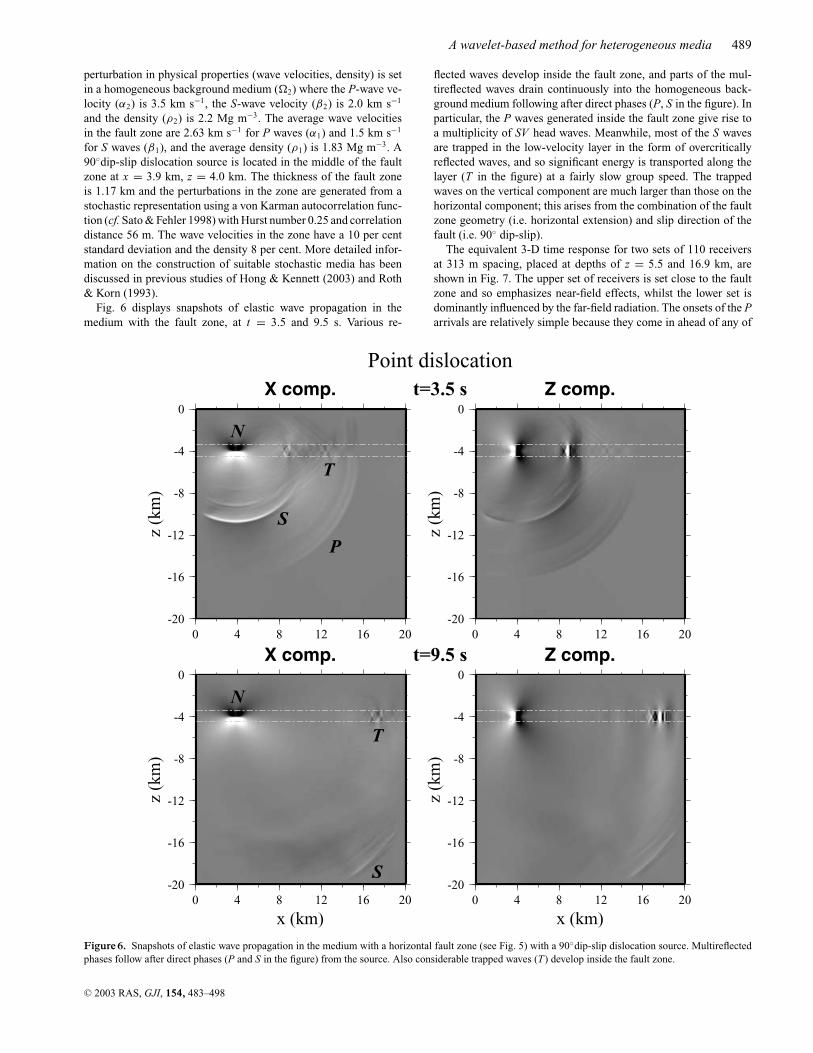
for S waves (β1), and the average density (ρ1) is 1.83 Mg m−3. A90dip-slip dislocation source is located in the middle of the faultzone at x = 3.9 km, z = 4.0 km. The thickness of the fault zoneis 1.17 km and the perturbations in the zone are generated from astochastic representation using a von Karman autocorrelation func-tion (cf. Sato & Fehler 1998) with Hurst number 0.25 and correlationdistance 56 m. The wave velocities in the zone have a 10 per centstandard deviation and the density 8 per cent. More detailed infor-mation on the construction of suitable stochastic media has beendiscussed in previous studies of Hong & Kennett (2003) and Roth& Korn (1993).
Fig. 6 displays snapshots of elastic wave propagation in themedium with the fault zone, at t = 3.5 and 9.5 s. Various re-
-20
-16
-12
-8
-4
0
z (k
m)
0 4 8 12 16 20-20
-16
-12
-8
-4
0
z (k
m)
0 4 8 12 16 20
-20
-16
-12
-8
-4
0
z (k
m)
0 4 8 12 16 20
x (km)
-20
-16
-12
-8
-4
0
z (k
m)
0 4 8 12 16 20
x (km)
Point dislocationt=3.5 s
t=9.5 s
X comp. Z comp.
X comp. Z comp.
N
N
T
T
S
P
S
Figure 6. Snapshots of elastic wave propagation in the medium with a horizontal fault zone (see Fig. 5) with a 90dip-slip dislocation source. Multireflectedphases follow after direct phases (P and S in the figure) from the source. Also considerable trapped waves (T) develop inside the fault zone.
flected waves develop inside the fault zone, and parts of the mul-tireflected waves drain continuously into the homogeneous back-ground medium following after direct phases (P, S in the figure). Inparticular, the P waves generated inside the fault zone give rise toa multiplicity of SV head waves. Meanwhile, most of the S wavesare trapped in the low-velocity layer in the form of overcriticallyreflected waves, and so significant energy is transported along thelayer (T in the figure) at a fairly slow group speed. The trappedwaves on the vertical component are much larger than those on thehorizontal component; this arises from the combination of the faultzone geometry (i.e. horizontal extension) and slip direction of thefault (i.e. 90 dip-slip).
The equivalent 3-D time response for two sets of 110 receiversat 313 m spacing, placed at depths of z = 5.5 and 16.9 km, areshown in Fig. 7. The upper set of receivers is set close to the faultzone and so emphasizes near-field effects, whilst the lower set isdominantly influenced by the far-field radiation. The onsets of the Parrivals are relatively simple because they come in ahead of any of
C© 2003 RAS, GJI, 154, 483–498

490 T.-K. Hong and B. L. N. Kennett
2
4
6
8
10
12
0 2 4 6 8 10 12 14 16 18 20
Tim
e (s
)
Range (km)
X
P+Pr
S+Sr
Tr
2
4
6
8
10
12
0 2 4 6 8 10 12 14 16 18 20
Tim
e (s
)
Range (km)
Z
2
4
6
8
10
12
0 2 4 6 8 10 12 14 16 18 20
Tim
e (s
)
Range (km)
X
P+Pr
S+Sr
2
4
6
8
10
12
0 2 4 6 8 10 12 14 16 18 20
Tim
e (s
)
Range (km)
Z
Figure 7. Time responses, with conversion to a 3-D response, at 110 receivers placed at (a) depth z = 5.5 (Rj in Fig. 5) and (b) 16.9 km (Dj) with an appropriateconversion procedure to the case of a point source. Multireflected phases (Pr, Sr) in a fault zone follow direct waves (P, S). Trapped waves interfere with randomheterogeneities in the fault zone, and leak into the background medium in a form of scattered waves (Tr).
the scattered arrivals, but the influence of the heterogeneity is seenin the significant S arrivals for the x component on the upper lineof receivers. The main trapped wave is of relatively low frequency,reflecting evanescent decay outside the fault-zone waveguide, butis accompanied by a higher-frequency coda with complex wave-forms from multiple scattering in the fault zone (Tr in the figure).A distinct complex of scattered energy is seen on the x-componentseismograms for small offsets from the source location. At largerdistances a more coherent set of arrivals follows S and becomesmore distinct for larger offsets.
The nature of the trapped wave phenomena can be most clearlyseen in a receiver profile across the fault zone as illustrated in Fig. 8.The lines are set at 4.7 and 13.0 km from the source. On the closerprofile, Fig. 8(a), there is still a significant influence from near-fieldeffects and the main part of the trapped wave train tends to mergewith the direct phases. The heterogeneity in the gouge zone leadsto an extended coda of backscattered waves on the z component.On the further line, Fig. 8(b), the nature of the trapping phenomenabecomes more evident. On the x component the fast P waves inthe surrounding material link into the slower P waves in the gougefrom which a significant SV head wave is being shed. The mainamplitude on the z component lies as expected in the S wave anddecays exponentially away from the fault zone so that relatively low-
frequency energy dominates at the receivers furthest from the faultzone, and a similar pattern was reported in Li & Leary (1990, Figs 7and 8). Part of the trapped waves consists of conversions betweenP and S and these are again prominent on the z component. Thepatterns of arrivals including long dispersed wave trains behind Sare similar to those recorded from aftershocks of the Hector Mineearthquake in California (Li et al. 2002) in a similar profile acrossthe fault zone. In this case the concentration of high-frequency ar-rivals was used as a means of mapping out the location of the faultzone.
4.3 Modelling with rupture propagation
In studies of ground motion in the vicinity of earthquakes it is nor-mally not adequate to approximate fault sources by a point dislo-cation source since the radiation patterns and frequency contentof the transient waves are strongly dependent not only on faultgeometry but also on the dynamic source process. For instance,Kasahara (1981) showed that radiation patterns vary with the ratio ofrupture velocity to shear wave velocity in the background mediumand they are shown to be elongated with an increase of rupturevelocity.
C© 2003 RAS, GJI, 154, 483–498

A wavelet-based method for heterogeneous media 491
0
2
4
6
8
10
6.5 6 5.5 5 4.5 4 3.5 3 2.5 2.0 1.5
Tim
e (s
)
Range (km)
X
0
2
4
6
8
10
6.5 6 5.5 5 4.5 4 3.5 3 2.5 2.0 1.5
Tim
e (s
)
Range (km)
Z
0
2
4
6
8
10
12
14
6.5 6 5.5 5 4.5 4 3.5 3 2.5 2.0 1.5
Tim
e (s
)
Range (km)
X
0
2
4
6
8
10
12
14
6.5 6 5.5 5 4.5 4 3.5 3 2.5 2.0 1.5
Tim
e (s
)
Range (km)
Z
Figure 8. Time responses, with conversion to 3-D response, for lines of receivers crossing the fault zone illustrating the nature of the trapped wave system inthe heterogeneous gouge zone (a) at x = 8.59 km (Ej in Fig. 5) and (b) at 16.88 km (K j) from the source.
-20
-16
-12
-8
-4
0
z (k
m)
0 4 8 12 16 20-20
-16
-12
-8
-4
0
z (k
m)
0 4 8 12 16 20
Rupture propagationt=3.5 sX comp. Z comp.
N
T
S
P
Figure 9. Snapshots of elastic wave propagation in a medium with a horizontal fault zone (Fig. 5) with a propagating 90dip-slip rupture. The same magnitudeof scalar moment M0 as in Fig. 6 is considered, and subsequent dislocations are considered in an area with horizontal extent 0.86 km. The permanent displacementpattern on the x component displays a horizontally extended shape following the rupture direction, but that on the z component is concentrated at the ends ofthe rupture.
C© 2003 RAS, GJI, 154, 483–498
492 T.-K. Hong and B. L. N. Kennett
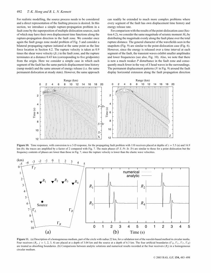
For realistic modelling, the source process needs to be consideredand a direct representation of the faulting process is desired. In thissection, we introduce a simple rupture-propagation problem in afault zone by the superposition of multiple dislocation sources, eachof which may have their own displacement time functions along therupture-propagation direction in the fault zone. We consider onceagain the fault gouge zone model problem of Fig. 5 and consider abilateral propagating rupture initiated at the same point as the lineforce location in Section 4.2. The rupture velocity is taken as 0.9times the shear wave velocity (β1) in the fault zone, and the ruptureterminates at a distance 0.43 km (corresponding to five gridpoints)from the origin. Here we consider a simple case in which eachsegment of the fault has the same particle displacement time history(ramp model) and the same amount of energy release (i.e. the samepermanent dislocation at steady state). However, the same approach
2
4
6
8
10
12
0 2 4 6 8 10 12 14 16 18 20
Tim
e (s
)
Range (km)
X
P+Pr
S+Sr
Tr
2
4
6
8
10
12
0 2 4 6 8 10 12 14 16 18 20
Tim
e (s
)
Range (km)
Z
Figure 10. Time responses, with conversion to a 3-D response, for the propagating fault problem with 110 receivers placed at depths of z = 5.5 (a) and 16.9km (b). the traces are amplified by a factor of 2 compared with Fig. 7. The main phases (P, S, Pr, Sr, Tr) are similar to those for a point dislocation but thefrequency contents of phases are lower than those in Fig. 7, since the rupture velocity is lower than the elastic wave velocities.
Source
R1
R2 R3 R4
543210-1-2-3-4-50
1
2
3
4
5
6
7
8
9
10
(km)
ΓRΓL
ΓB
ΓT
0 1 2 3 4 5 0 1 2 3 4 5
Time (s)
R1 R2
R3 R4
numericalanalytic
Figure 11. (a) Description of a homogeneous medium, part of the circle with radius 22 km, for a validation test of the wavelet-based method in circular media.Four receivers (Rj, j = 1, 2, 3, 4) are placed at a depth of 3.04 km and the source at a depth of 6.3 km. The four artificial boundaries (R , L , T , B )are treated as absorbing boundaries. (b) Comparisons between analytic solutions and numerical results recorded at the four receivers (Rj) in a homogeneouscircular medium.
can readily be extended to much more complex problems whereevery segment of the fault has own displacement time history andenergy release rate.
For comparison with the results of the point-dislocation case (Sec-tion 4.2), we consider the same magnitude of seismic moment M0 bydistributing the magnitude evenly along the fault plane over the totalrupture distance. The general character of the wavefields seen in thesnapshots (Fig. 9) are similar to the point-dislocation case (Fig. 6).However, since the energy is released over a time interval at eachsegment of the fault, the transient waves exhibit smaller amplitudesand lower frequencies (see also, Fig. 10). Also, we note that thereis now a much weaker P disturbance in the fault zone and conse-quently much fewer in the way of S head waves in the surroundings.The permanent displacement patterns (N in Fig. 9) around the faultdisplay horizontal extension along the fault propagation direction
C© 2003 RAS, GJI, 154, 483–498
A wavelet-based method for heterogeneous media 493
(km)
S1
S2
hθ
ΓR
ΓL
ΓT
ΓB
-150 -100 -50 0 50 100 150
0
50
100
150
a
b
A
B
A
B
b
a
case Acase B
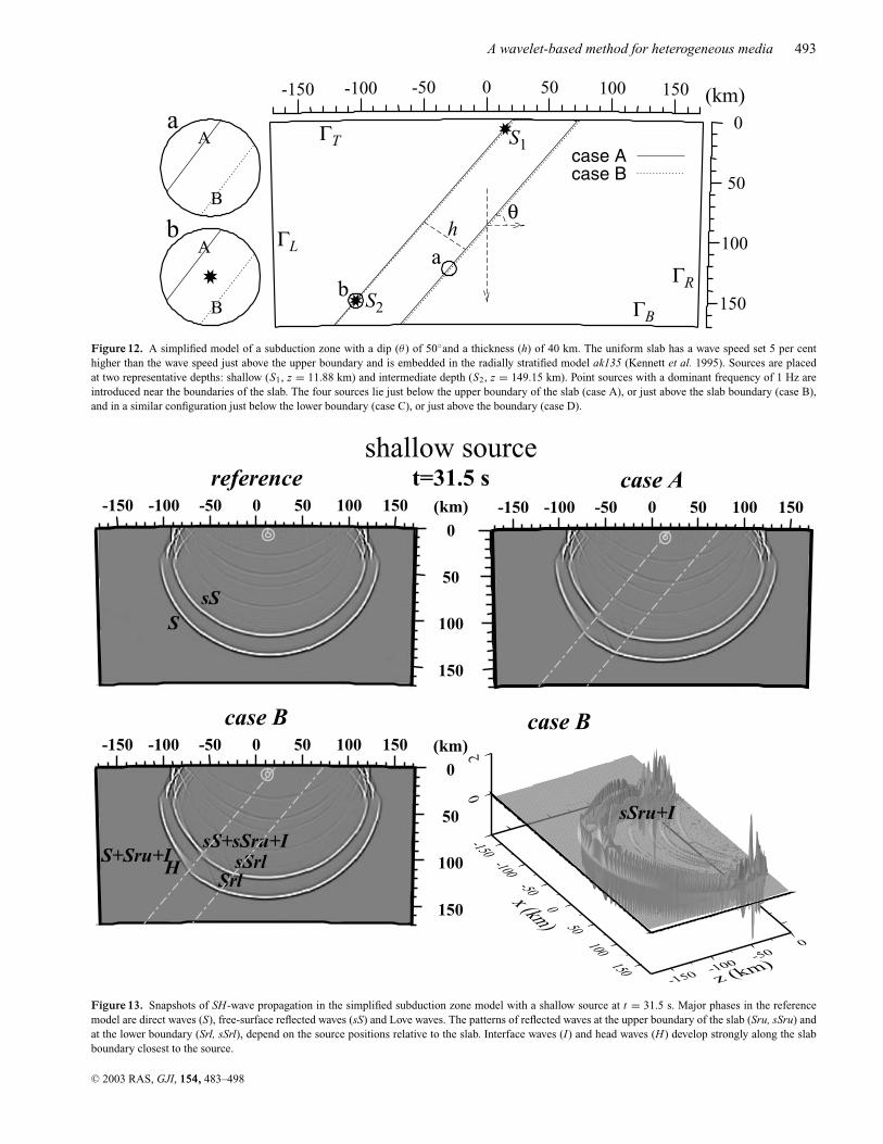
Figure 12. A simplified model of a subduction zone with a dip (θ ) of 50and a thickness (h) of 40 km. The uniform slab has a wave speed set 5 per centhigher than the wave speed just above the upper boundary and is embedded in the radially stratified model ak135 (Kennett et al. 1995). Sources are placedat two representative depths: shallow (S1, z = 11.88 km) and intermediate depth (S2, z = 149.15 km). Point sources with a dominant frequency of 1 Hz areintroduced near the boundaries of the slab. The four sources lie just below the upper boundary of the slab (case A), or just above the slab boundary (case B),and in a similar configuration just below the lower boundary (case C), or just above the boundary (case D).
-150 -100 -50 0 50 100 150
0
50
100
150
(km)
referenceshallow source
t=31.5 s
SsS
-150 -100 -50 0 50 100 150
case A
-150 -100 -50 0 50 100 150
0
50
100
150
(km)
case B
SrlsSrlS+Sru+I
sS+sSru+I
H
-150-100
-500
50100
150
x (km)
-150 -100-50
0
z (km)
02
case B
sSru+I
Figure 13. Snapshots of SH-wave propagation in the simplified subduction zone model with a shallow source at t = 31.5 s. Major phases in the referencemodel are direct waves (S), free-surface reflected waves (sS) and Love waves. The patterns of reflected waves at the upper boundary of the slab (Sru, sSru) andat the lower boundary (Srl, sSrl), depend on the source positions relative to the slab. Interface waves (I) and head waves (H) develop strongly along the slabboundary closest to the source.
C© 2003 RAS, GJI, 154, 483–498

494 T.-K. Hong and B. L. N. Kennett
in the x components. In contrast the permanent displacements areconcentrated at the end of the rupture on the z component and arenot discernible along the plane of rupture.
The time responses in Fig. 10 for the propagating rupture sourceare displayed with twice the amplification used in Fig. 7. The mul-tiple reflected waves following S waves for receivers at short offseton the x components for the point dislocation case (Fig. 7) do notappear in the profiles for propagating rupture.
5 M O D E L L I N G I NS U B D U C T I O N Z O N E S
A further region in which sources occur within a zone of hetero-geneity is in the coherent and systematic high-velocity zone of thesubducting slab. The majority of earthquakes associated with thesubduction zone lie within the slab but relatively close to its up-per surface. Seismic waves generated from such sources within theslab have the potential of strong interaction with the slab boundarieswith reflections and conversions. There is also the possibility of in-terface waves associated with the contrasts in properties at the edgeof the slab. The combination of the effects introduced by the slab canhave significant effects on the local wavefield and also have the po-tential to modify the high-frequency characteristics for teleseismicpropagation.
Waveform and amplitude variations of incident waves prop-agating through a slab have been studied at regional distance
-150 -100 -50 0 50 100 150
0
50
100
150
(km)
referenceintermediate-depth source
t=31.5 s
S
-150 -100 -50 0 50 100 150
case A
S+Sru+I
-150 -100 -50 0 50 100 150
0
50
100
150
(km)
case B
H
Srl
Figure 14. Snapshots of SH-wave propagation in subduction zones with an intermediate depth of source at t = 31.5s. The wavefields are simpler than thosein Fig. 14, but the phases developing on boundaries are clearly shown to travel into the free surface. The main reflected waves (Sru, Srl), interface waves (I)and head waves (H) are indicated.
with both numerical modelling (e.g. Cormier 1989; Sekiguchi1992; Kennett & Furumura 2002) and observational analysis(Lay & Young 1989). Recently, waveguide effects in the accre-tionary prism above the slab have been investigated by Shapiroet al. (2000). However, the generation of secondary waves insubduction zones (such as reflected waves, interface waves) havenot received much attention. Moreover, when waves interferewith a fast-velocity layer placed between low-velocity layers,it is possible to get tunnelling effects (Fuchs & Schulz 1976;Drijkoningen 1991), which depend on the frequency content of thewavefield and the thickness of the layer, which can contribute towaveform complexity. Thus, low-frequency waves with large wave-length are hardly affected by the presence of the subducting slab butthe impact increases at higher frequencies.
We consider the SH-wave case at a regional scale, and show howthe WBM method can be used to handle the presence of a simpli-fied subduction zone embedded in a radially stratified backgroundmodel, including secondary wave effects.
The subduction zone structure extends to such a depth that we can-not ignore the influence of the sphericity of the Earth and so needto adapt the WBM to a non-Cartesian coordinate system. Spheri-cal finite-difference methods have been introduced for the simula-tion of SH waves in the mantle (Igel & Weber 1995; Chaljub &Tarantola 1997) and P–SV (Igel & Weber 1996) wave propagationin the sphere. An alternative approach, which remains in 2-D, wasadopted by Furumura et al. (1998) with a cylindrical-coordinate
C© 2003 RAS, GJI, 154, 483–498

A wavelet-based method for heterogeneous media 495
representation for P–SV -wave equations in modelling using apseudospectral method. For a 2-D structure such as a subductingplate, modelling with a spherical coordinate system, requires thepole axis to be treated by a symmetry condition, with a vanishingdisplacement vector on the axis, and thus an additional boundarycondition is needed. To preserve the simplicity of the situation weuse cylindrical coordinates for SH waves with the background radi-ally stratified model based on ak135 (Kennett et al. 1995).
5.1 Numerical implementation
The SH-wave equation in a cylindrical coordinate (r , θ , y) system(cf. Aki & Richards 1980) takes the form
∂2uy
∂t2= 1
ρ
(σr
r+ ∂σr
∂r+ 1
r
∂σθ
∂θ+ fy
), (12)
where the stress terms σ r and σ θ are given by
σr = µ∂uy
∂r, σθ = µ
r
∂uy
∂θ. (13)
This set of equations for SH can be recast in the wavelet represen-tation in a similar way to that in Sections 2 and 3, working withnormalized radius.
The traction-free condition at the free surface and the core–mantleboundary (if applicable) is σ r = 0, and this can be implemented viaequivalent forces in N, eq. (5), as in Hong & Kennett (2002a).
5.2 Validation tests
The accuracy of the wavelet-based method in cylindrical coordinateshas been tested with a variety of models where analytic solutions areavailable. We illustrate these tests for a cylinder with small radiuswhere the influence of curvature is strong.
10
20
30
40
50
60
0 40 80 120 160-40-80-120-160
Tim
e (s
)
reference
Range (km)
10
20
30
40
50
60
0 40 80 120 160-40-80-120-160
Tim
e (s
)
reference - case A
Range (km)
10
20
30
40
50
60
0 40 80 120 160-40-80-120-160
Tim
e (s
)
case A - case B
Range (km)
Figure 15. Seismograms at the surface for shallow sources in the simplified subduction model. (a) The main features of the seismograms are well representedby the reference model. The features associated with the presence of the slab are enhanced by considering difference seismograms. The main features of sourcepositions at the upper and lower slab boundaries can be seen from (b) reference case A (upper), (c) reference case C (lower). The more subtle differences arisingfrom the position of the source, inside or outside the slab, are apparent from the difference seismograms (d) case A–case B and (e) case C–case D. The maindifferences arise from the time advance of the waves in the slab models when they pass through the slab. Reflected arrivals from the upper boundary of the slabare important for sources near the upper boundary, and are more pronounced for case B where the source lies outside the slab.
We consider a portion of a uniform cylinder with radius 22 km(Fig. 11a). Four artificial boundaries (R , L , T , B) are treatedby absorbing boundary conditions. Four receivers (Rj, j = 1, 2, 3, 4)are placed at a depth of 3.04 km in a row with interval 1.61 km, anda point force is applied at a depth of 6.3 km. The numerical modelis represented with 128 × 128 gridpoints, the shear wave velocity isset to be 2.0 km s−1, and the density 2.2 Mg m−3. A Ricker waveletwith dominant frequency 4.5 Hz is implemented for the source timefunction.
As shown in Fig. 11(b), the wavelet-based method generatestime responses with correct traveltimes and amplitudes for this uni-form cylinder case. A barely noticeable high-frequency jitter distin-guishes the numerical simulation from the analytical results.
A similar comparison has been made for both the effects of thefree surface and layering for model segments placed at the surfaceof the Earth so that curvature effects are minimized. The replicationof the analytic results matches that of Fig. 11(b) and so confirmsthe accuracy of the cylindrical WBM method. For more complexstratified models analytic solutions are not available but a strongcheck on the validity of the WBM method is provided by the precisematch of the wave front patterns for both shallow and deep sources.
5.3 SH waves in subduction zones
The geometry of subducting slabs is approximately 2-D, but thevelocity anomalies revealed by seismic tomography indicate thatthere can be significant variations along a single subduction zone(e.g. Pankow & Lay 2002; Kennett 2002; Widiyantoro et al.1999;Ding & Grand 1994).
Here we implement a simplified slab model based on a recentstudy (Pankow & Lay 2002) of shear wave velocity structure inthe Kurile subduction zone. We consider a slab with a dip (θ ) of
C© 2003 RAS, GJI, 154, 483–498
496 T.-K. Hong and B. L. N. Kennett
25 30 35 40 45
Time (s)
shallow source
x= -100.0 km
x= 116.2 km
referencecase Acase B
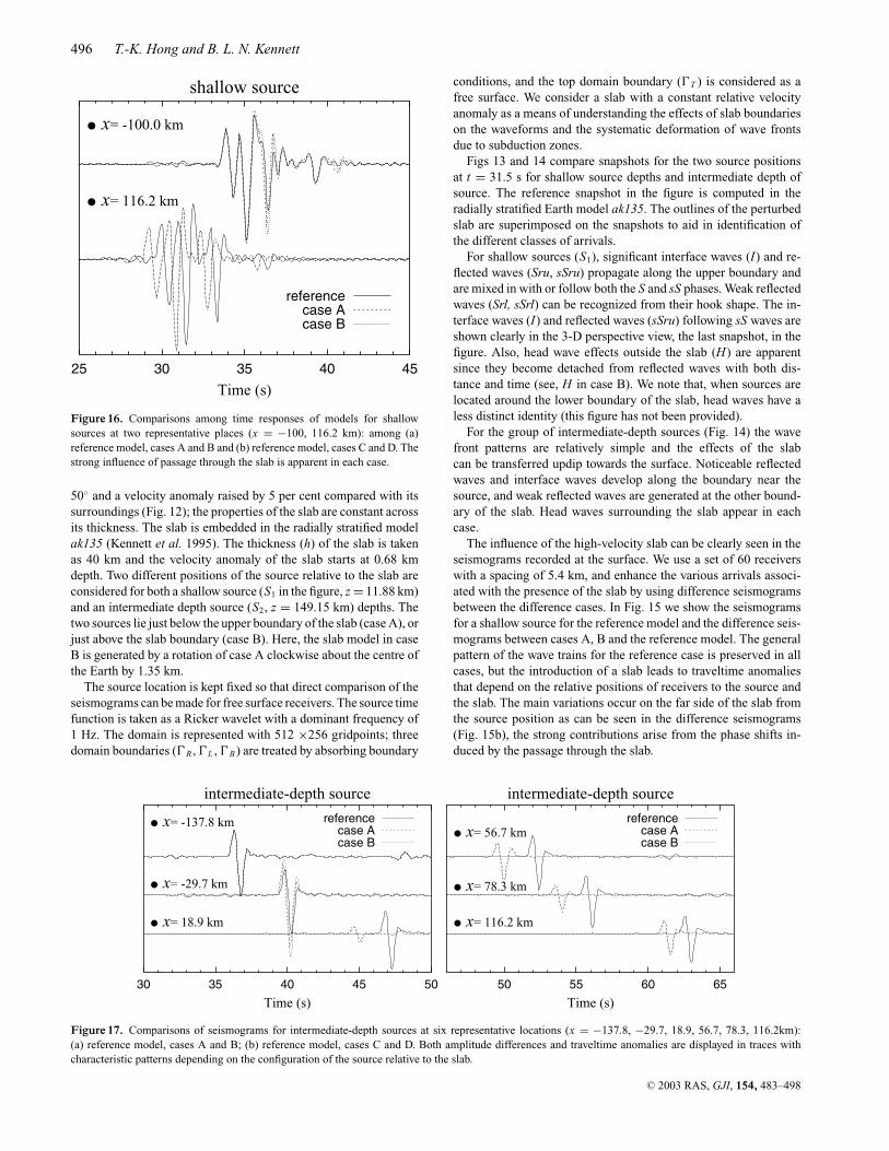
Figure 16. Comparisons among time responses of models for shallowsources at two representative places (x = −100, 116.2 km): among (a)reference model, cases A and B and (b) reference model, cases C and D. Thestrong influence of passage through the slab is apparent in each case.
50 and a velocity anomaly raised by 5 per cent compared with itssurroundings (Fig. 12); the properties of the slab are constant acrossits thickness. The slab is embedded in the radially stratified modelak135 (Kennett et al. 1995). The thickness (h) of the slab is takenas 40 km and the velocity anomaly of the slab starts at 0.68 kmdepth. Two different positions of the source relative to the slab areconsidered for both a shallow source (S1 in the figure, z = 11.88 km)and an intermediate depth source (S2, z = 149.15 km) depths. Thetwo sources lie just below the upper boundary of the slab (case A), orjust above the slab boundary (case B). Here, the slab model in caseB is generated by a rotation of case A clockwise about the centre ofthe Earth by 1.35 km.
The source location is kept fixed so that direct comparison of theseismograms can be made for free surface receivers. The source timefunction is taken as a Ricker wavelet with a dominant frequency of1 Hz. The domain is represented with 512 ×256 gridpoints; threedomain boundaries (R , L , B) are treated by absorbing boundary
30 35 40 45 50
Time (s)
intermediate-depth source
x= -137.8 km
x= -29.7 km
x= 18.9 km
referencecase Acase B
50 55 60 65
Time (s)
intermediate-depth source
x= 56.7 km
x= 78.3 km
x= 116.2 km
referencecase Acase B
Figure 17. Comparisons of seismograms for intermediate-depth sources at six representative locations (x = −137.8, −29.7, 18.9, 56.7, 78.3, 116.2km):(a) reference model, cases A and B; (b) reference model, cases C and D. Both amplitude differences and traveltime anomalies are displayed in traces withcharacteristic patterns depending on the configuration of the source relative to the slab.
conditions, and the top domain boundary (T ) is considered as afree surface. We consider a slab with a constant relative velocityanomaly as a means of understanding the effects of slab boundarieson the waveforms and the systematic deformation of wave frontsdue to subduction zones.
Figs 13 and 14 compare snapshots for the two source positionsat t = 31.5 s for shallow source depths and intermediate depth ofsource. The reference snapshot in the figure is computed in theradially stratified Earth model ak135. The outlines of the perturbedslab are superimposed on the snapshots to aid in identification ofthe different classes of arrivals.
For shallow sources (S1), significant interface waves (I) and re-flected waves (Sru, sSru) propagate along the upper boundary andare mixed in with or follow both the S and sS phases. Weak reflectedwaves (Srl, sSrl) can be recognized from their hook shape. The in-terface waves (I) and reflected waves (sSru) following sS waves areshown clearly in the 3-D perspective view, the last snapshot, in thefigure. Also, head wave effects outside the slab (H) are apparentsince they become detached from reflected waves with both dis-tance and time (see, H in case B). We note that, when sources arelocated around the lower boundary of the slab, head waves have aless distinct identity (this figure has not been provided).
For the group of intermediate-depth sources (Fig. 14) the wavefront patterns are relatively simple and the effects of the slabcan be transferred updip towards the surface. Noticeable reflectedwaves and interface waves develop along the boundary near thesource, and weak reflected waves are generated at the other bound-ary of the slab. Head waves surrounding the slab appear in eachcase.
The influence of the high-velocity slab can be clearly seen in theseismograms recorded at the surface. We use a set of 60 receiverswith a spacing of 5.4 km, and enhance the various arrivals associ-ated with the presence of the slab by using difference seismogramsbetween the difference cases. In Fig. 15 we show the seismogramsfor a shallow source for the reference model and the difference seis-mograms between cases A, B and the reference model. The generalpattern of the wave trains for the reference case is preserved in allcases, but the introduction of a slab leads to traveltime anomaliesthat depend on the relative positions of receivers to the source andthe slab. The main variations occur on the far side of the slab fromthe source position as can be seen in the difference seismograms(Fig. 15b), the strong contributions arise from the phase shifts in-duced by the passage through the slab.
C© 2003 RAS, GJI, 154, 483–498

A wavelet-based method for heterogeneous media 497
Reflected waves from the upper boundary of the slab also playan important role in the waveform variation in the later part of thewave trains recorded above the slab in a narrow interval x = −60 to−140 km, Fig. 15(b), corresponding to ranges of 80–160 km fromthe epicentre. For the source inside the slab (case A) the reflectedwaves are mainly generated by sS waves, but for an external source(case B) both S and sS waves contribute and the amplitude is en-hanced (see Figs 15b and c for x = −100.0 km).
The waveforms for a shallow source at two locations are comparedin Fig. 16. At x = −100 km, the influence of the reflected waves forthe upper boundary of the slab can be seen in the modification ofthe later part of the main pulse. With the observation point on theother side of the slab at x = 116.2 km, there is a bulk shift of thewaveforms.
For an intermediate depth source a rather different pattern of ar-rivals is produced. Although the slab offers a fast propagation path,energy is continuously shed from the high-velocity slab into thelower-velocity surroundings (note the weakened wave fronts in theslab in Fig. 14). As a result the waves emerging at the surface in theslab zone are advanced in time but show rather small amplitudescompared with the reference case (Fig. 17 at x = 18.9 km). Directtransmission through the slab also induces some loss in amplitudedue to the contrasts at the slab boundaries (at x = 78.3, 116.2 km).Reflected waves can contribute to local enhancement of the ampli-tude just outside the slab zone (x = −29.7 km).
6 D I S C U S S I O N A N D C O N C L U S I O N S
The wavelet-based method (WBM) provides an effective means ofsimulating elastic wave propagation in heterogeneous media, sinceit can cope with rapid variations in physical properties without lossof accuracy. With the improved scheme for source representationintroduced in this paper it is possible to place moment-tensor or dis-location sources directly in regions of heterogeneity. This enablesthe WBM to be used effectively in a variety of problems where sig-nificant contrasts in physical properties occur in the neighbourhoodof the source.
In the case of sources within a highly heterogeneous fault gougezone, we get strong waveguide effects for P–SV waves, whichare modified somewhat when we introduce a propagating rupture.The fault-trapped waves decay outside the fault zone and the pres-ence of high-frequency energy provides a good guide to the locationof the fault zone itself.
In subduction zones, the slab represents a region of elevated wavespeed compared with its surroundings. Although propagation alongthe slab is fast, substantial energy is shed in an antiwaveguide effect.The contrasts at the boundaries of the slab have the potential togenerate reflected and interface phases that can add to the complexityof the seismograms for stations in the vicinity of the slab.
A C K N O W L E D G M E N T S
This paper has benefited from the helpful review comments of DrsYong-Gang Li, Heiner Igel and Michael Korn (editor). Also, wethank the Australian National University Supercomputer Facilityfor allocation of computer time on the Alpha server.
R E F E R E N C E S
Aki, K. & Richards, P.G., 1980. Quantitative Seismology, Theory and Meth-ods, Vol. 1, Freeman, San Francisco.
Alterman, Z. & Karal, F.C., Jr, 1968. Propagation of elastic waves in layeredmedia by finite difference methods, Bull. seism. Soc. Am., 58, 367–398.
Ben-Menahem, A. & Singh, S.J., 1981. Seismic Waves and Sources, Springer-Verlag, New York.
Ben-Zion, Y., 1998. Properties of seismic fault zone waves and their utilityfor imaging low-velocity structures, J. geophys. Res., 103, 12 567–12 585.
Ben-Zion, Y. & Aki, K., 1990. Seismic radiation from an SH line sourcein a laterally heterogeneous planar fault zone, Bull. seism. Soc. Am., 80,971–994.
Beylkin, G., 1992. On the representation of operators in bases of compactlysupported wavelets, SIAM J. Numer. Anal., 6, 1716–1740.
Beylkin, G. & Keiser, J.M., 1997. On the adaptive numerical solution ofnonlinear partial differential equations in wavelet bases, J. Comput. Phys.,132, 233–259.
Chaljub, E. & Tarantola, A., 1997. Sensitivity of SS precursors to topographyon the upper-mantle 660-km discontinuity, Geophys. Res. Lett., 24, 2613–2616.
Cormier, V.F., 1989. Slab diffraction of S waves, J. geophys. Res., 94, 3006–3024.
Coutant, O., Virieux, J. & Zollo, A., 1995. Numerical source implementationin a 2-D finite difference scheme, Bull. seism. Soc. Am., 85, 1507–1512.
Ding, X.-Y. & Grand, S.P., 1994. Seismic structure of the deep kurile sub-duction zone, J. Geophys. Res., 99(B12), 23, 767–786.
Drijkoningen, G.G., 1991. Tunnelling and the generalized ray method inpiecewise homogeneous media, Geophys. Prospect., 39, 757–781.
Falk, J., Tessmer, E. & Gajewski, D., 1998. Efficient finie-difference mod-elling of seismic waves using locally adjustable time steps, Geophys.Prospect., 46, 603–616.
Fuchs, K. & Schulz, K., 1976. Tunneling of low-frequency waves throughthe subcrustal lithosphere, J. Geophys., 42, 175–190.
Furumura, T. & Kennett, B.L.N., 1998. On the nature of regional seismicphases—III. The influence of crustal heterogeneity on the wavefield forsubduction earthquakes: the 1985 Michoacan and 1995 Copala, Guerrero,Mexico earthquakes, Geophys. J. Int., 135, 1060–1084.
Furumura, T., Kennett, B.L.N. & Furumura, M., 1998. Seismic wavefieldcalculation for laterally heterogeneous whole Earth models using the pseu-dospectral method, Geophys. J. Int., 135, 845–860.
Graves, R.W., 1996. Simulating seismc wave propagation in 3-D elasticmedia using staggered-grid finite differences, Bull. seism. Soc. Am., 86,1091–1106.
Hong, T.-K. & Kennett, B.L.N., 2002a. A wavelet-based method for simula-tion of two-dimensional elastic wave propagation, Geophys. J. Int., 150,610–638.
Hong, T.-K. & Kennett, B.L.N., 2002b. On a wavelet-based method for thenumerical simulation of wave propagation, J. Comput. Phys., 183, 577–622.
Hong, T.-K. & Kennett, B.L.N., 2003. Scattering attenuation of 2D elasticwaves: theory and numerical modeling using a wavelet-based method,Bull. seism. Soc. Am., 93, 922–938.
Hough, S.E., Ben-Zion, Y. & Leary, P., 1994. Fault-zone waves observed atthe Southern Joshua Tree earthquake rupture zone, Bull. seism. Soc. Am.,84, 761–767.
Huang, B.-S., Teng, T.-L. & Yeh, Y.T., 1995. Numerical modeling of fault-zone trapped waves: acoustic case, Bull. seism. Soc. Am., 85, 1711–1717.
Igel, H., Mora, P. & Riollet, B., 1995. Anisotropic wave propagation throughfinite-difference grids, Geophysics, 60, 1203–1216.
Igel, H., Ben-Zion, Y. & Leary, P.C., 1997. Simulation of SH- andP–SV-wave propagation in fault zones, Geophys. J. Int., 128, 533–546.
Igel, H., Jahnke, G. & Ben-Zion, Y., 2002. Numerical simulation of faultzone guided waves: accuracy and 3-D effects, Pure appl. Geophys., 159,2067–2083.
Igel, H. & Weber, M., 1995. SH–wave propagation in the whole mantle usinghigh-order finite differences, Geophys. Res. Lett., 22, 731–734.
Igel, H. & Weber, M., 1996. P–SV–wave propagation in the Earth’s mantleusing finite differences: applications to heterogeneous lowermost mantlestructure, Geophys. Res. Lett., 23, 415–418.
Jahnke, G., Igel, H. & Ben-Zion, Y., 2002. Three-dimensional calculationsof fault-zone-guided waves in various irregular structures, Geophys. J.Int., 151, 416–426.
C© 2003 RAS, GJI, 154, 483–498
498 T.-K. Hong and B. L. N. Kennett
Kasahara, K., 1981. Earthquake Mechancis, Cambridge University Press,Cambridge.
Kaser, M. & Igel, H., 2001. Numerical simulation of 2-D wave propaga-tion on unstructured grids using explicit differential operators, Geophys.Prospect., 49, 607–619.
Kelly, K.R., Ward, R.W., Treitel, S. & Alford, R.M., 1976. Synthetic sismo-grams: a finite-difference approach, Geophysics, 41, 2–27.
Kennett, B.L.N., 2001. Seismic Wavefield, vol. I:Introduction and Theoreti-cal Development, p. 370, Cambridge University Press, New York.
Kennett, B.L.N., 2002. Seismic Wavefield, vol. II: Interpretation of Seis-mograms on Regional and Global Scales, p. 534, Cambridge UniversityPress, New York.
Kennett, B.L.N. & Furumura, T., 2002. The influence of 3-D structure onthe propagation of seismic waves away from earthquakes, Pure appl. Geo-phys., 159, 2113–2131.
Kennett, B.L.N., Engdahl, E.R. & Buland, R., 1995. Constraints on seismicvelocities in the Earth from travel times, Geophys. J. Int., 122, 108–124.
Komatitsch, D. & Tromp, J., 2002. Spectral-element simulations of globalseismic wave propagation—I. Validation, Geophys. J. Int., 149, 390–412.
Kosloff, D., Reshef, M. & Loewenthal, D., 1984. Elastic wave calcuationsby the Fourier method, Bull. seism. Soc. Am., 74, 875–891.
Kosloff, D., Kessler, D., Filho, A.Q., Tessmer, E., Behle, A. & Strahilevitz,R., 1990. Solution of the equations of dynamic elasticity by a Chebychevspectral method, Geophysics, 55, 734–748.
Lay, T. & Wallace, T.C., 1995. Modern Global Seismology, Academic, NewYork.
Lay, T. & Young, C.J., 1989. Waveform complexity in teleseismic broadbandSH displacements: slab diffractions or deep mantle reflections?, Geophys.Res. Lett., 16, 605–608.
Levander, A.R., 1988. Fourth-order finite-difference P–SV seismograms,Geophysics, 53, 1425–1436.
Li, Y.-G., 1988. Trapped modes in a transversely isotropic fault-zone, PhDthesis, pp. 168–189, University of Southern California.
Li, Y.-G. & Leary, P.C., 1990. Fault zone trapped seismic waves, Bull. seism.Soc. Am., 80, 1245–1271.
Li, Y.-G. & Vidale, J.E., 1996. Low-velocity fault-zone guided waves: nu-merical investigations of trapping efficiency, Bull. seism. Soc. Am., 86,371–378.
Li, Y.-G., Leary, P.C., Aki, K. & Malin, P.E., 1990. Seismic trapped modesin the Oroville and San Andreas fault zones, Science, 249, 763–766.
Li, Y.-G., Aki, K., Vidale, J.E. & Xu, F., 1999. Shallow structure of theLanders fault zone from explosion-generated trapped waves, J. geophys.Res., 104, 20 257–20 275.
Li, Y.-G., M., Vidale, J.E., Day, S.M., Oglesby, D.D. & the SCEC FieldWorking Team, 2002. Study of the 1999 M 7.1 Hector mine, California,earthquake fault plane by trapped waves, Bull. seism. Soc. Am., 92, 1318–1332.
Pankow, K.L. & Lay, T., 2002. Modeling, S wave amplitude patterns forevents in the Kurile slab using three-dimensional Gaussian beams, J. geo-phys. Res., 107, 10.1029/2001JB000594.
Roth, M. & Korn, M., 1993. Single scattering theory versus numerical mod-elling in 2-D random media, Geophys. J. Int., 112, 124–140.
Sato, H. & Fehler, M.C., 1998. Seismic Wave Propagation and Scattering inthe Heterogeneous Earth, Springer-Verlag, New York.
Sekiguchi, S., 1992. Amplitude distribution of seismic waves for laterallyheterogeneous structures including a subducting slab, Geophys. J. Int.,111, 448–464.
Shapiro, N.M., Olsen, K.B. & Singh, S.K., 2000. Wave-guide effects insubduction zones: evidence from three-dimensional modeling, Geophys.Res. Lett., 27, 433–436.
Vidale, J.E., 1987. Waveform effects of a high-velocity, subducted slab,Geophys. Res. Lett., 15, 542–545.
Vidale, J., Helmberger, D.V. & Clayton, R.W., 1985. Finite-difference seis-mograms for SH waves, Bull. seism. Soc. Am., 75, 1765–1782.
Widiyantoro, S., Kennett, B.L.N. & van der Hilst, R.D., 1999. Seismic to-mography with P and S data reveals lateral variations in the rigidity ofdeep slabs, Earth planet. Sci. Lett., 173, 91–100.
Yomogida, K. & Etgen, J.T., 1993. 3-D wave propagation in the Los AngelesBasin for the Whittier–Narrows earthquake, Bull. seism. Soc. Am., 83,1325–1344.
C© 2003 RAS, GJI, 154, 483–498