Embed Size (px)
Citation preview

Atmos. Chem. Phys., 12, 8499–8527, 2012www.atmos-chem-phys.net/12/8499/2012/doi:10.5194/acp-12-8499-2012© Author(s) 2012. CC Attribution 3.0 License.
AtmosphericChemistry
and Physics
Modelling of organic aerosols over Europe (2002–2007) using avolatility basis set (VBS) framework: application of differentassumptions regarding the formation of secondary organic aerosol
R. Bergstrom1,2, H. A. C. Denier van der Gon3, A. S. H. Prevot4, K. E. Yttri 5, and D. Simpson6,7
1Department of Chemistry and Molecular Biology, University of Gothenburg, 41296 Gothenburg, Sweden2Swedish Meteorological and Hydrological Institute, 60176 Norrkoping, Sweden3TNO Netherlands Organisation for Applied Scientific Research, Utrecht, The Netherlands4Laboratory of Atmospheric Chemistry, Paul Scherrer Institut, Villigen, Switzerland5Norwegian Institute for Air Research, Kjeller, Norway6EMEP MSC-W, Norwegian Meteorological Institute, Oslo, Norway7Dept. Earth & Space Sciences, Chalmers Univ. Technology, Gothenburg, Sweden
Correspondence to:D. Simpson ([email protected])
Received: 3 January 2012 – Published in Atmos. Chem. Phys. Discuss.: 20 February 2012Revised: 20 August 2012 – Accepted: 6 September 2012 – Published: 21 September 2012
Abstract. A new organic aerosol module has been imple-mented into the EMEP chemical transport model. Four dif-ferent volatility basis set (VBS) schemes have been testedin long-term simulations for Europe, covering the six years2002–2007. Different assumptions regarding partitioning ofprimary organic aerosol and aging of primary semi-volatileand intermediate volatility organic carbon (S/IVOC) speciesand secondary organic aerosol (SOA) have been explored.Model results are compared to filter measurements, aerosolmass spectrometry (AMS) data and source apportionmentstudies, as well as to other model studies. The present studyindicates that many different sources contribute significantlyto organic aerosol in Europe. Biogenic and anthropogenicSOA, residential wood combustion and vegetation fire emis-sions may all contribute more than 10 % each over substan-tial parts of Europe. This study shows smaller contributionsfrom biogenic SOA to organic aerosol in Europe than ear-lier work, but relatively greater anthropogenic SOA. SimpleVBS based organic aerosol models can give reasonably goodresults for summer conditions but more observational stud-ies are needed to constrain the VBS parameterisations andto help improve emission inventories. The volatility distribu-tion of primary emissions is one important issue for furtherwork. Emissions of volatile organic compounds from bio-genic sources are also highly uncertain and need further vali-
dation. We can not reproduce winter levels of organic aerosolin Europe, and there are many indications that the presentemission inventories substantially underestimate emissionsfrom residential wood combustion in large parts of Europe.
1 Introduction
During the last 10–15 yr carbonaceous aerosol has becomeone of the most intensively studied fields within the at-mospheric sciences. This can be attributed to its postu-lated impacts on global climate (Novakov and Penner, 1993;Kanakidou et al., 2005), and on human health (McDonaldet al., 2004). Particulate carbonaceous matter (PCM) con-tributes around 10–40 % (mean 30 %) to the total concentra-tion of particulate matter (PM) with diameter less than 10 µm(PM10) at rural and natural background sites in Europe (Yt-tri et al., 2007; Putaud et al., 2004). PCM consists largely oforganic matter (OM, of which typically 40–80 % is OC: or-ganic carbon (Turpin and Lim, 2001; El-Zanan et al., 2009),with the rest made up of associated oxygen, hydrogen, andother atoms) and so-called elemental or black carbon (EC orBC). The sum of EC and OC is referred to as total carbon(TC). OM is a very important fraction of sub-micron parti-cles (PM1) as well. In a recent aerosol mass spectrometry
Published by Copernicus Publications on behalf of the European Geosciences Union.

8500 R. Bergstrom et al.: Modelling organic aerosol over Europe 2002–2007
(AMS) study of non-refractory (NR) PM1 in Central Europe,Lanz et al.(2010) found that about 40–80 % of the NR-PM1was made up of OM.
The EMEP EC/OC model has previously been presentedby Simpson et al.(2007); two versions of a gas-particlescheme for secondary organic aerosol (SOA) were used,Kam-2 from Andersson-Skold and Simpson(2001), anda modification, Kam-2X, which use alternative “effective”vapour pressures, for the semi-volatile organic aerosol com-pounds, to increase partitioning to the particulate phase.Model results were compared with measurements from theEMEP EC/OC campaign (Yttri et al., 2007) and the EUCARBOSOL project (Legrand and Puxbaum, 2007). Com-parisons were also made of the different components of TC,e.g. anthropogenic and biogenic secondary organic aerosols(ASOA, BSOA) from emitted volatile organic compounds,against observation-based estimates of these compoundsmade byGelencser et al.(2007).
The study demonstrated that the Kam-2 and Kam-2Xschemes were able to predict observed levels of OC in North-ern Europe fairly well, but for southern Europe the modelunderestimated OC significantly. In wintertime, the under-prediction was shown to be caused by problems with wood-burning emissions (possibly local). In summer the problemswere due to an under-prediction of the SOA components. Themodel results were very sensitive to assumptions concerningthe vapour pressures of the model compounds.
As discussed in, e.g.Hallquist et al.(2009), the sourcesand formation mechanisms of SOA are still very uncertain,with many plausible pathways but still no reliable estimatesof their relative importance. In such a situation one cannotexpect a model to accurately reproduce measurements. Still,it is important to understand the extent to which models orparameterisations derived from smog-chambers can captureobserved levels and variations in OC.
Donahue and co-workers introduced the use of a volatilitybasis set (VBS) to help models cope with the wide range oforganic aerosol species and the oxidation of organics of dif-ferent volatilities in the atmosphere (see, e.g.Donahue et al.,2006, 2009). This scheme is suitable for regional and globalscale modelling of organic aerosol as it provides a convenientframework with the aerosol described by a physically plau-sible range of properties, and simple relationships governingpartitioning and transformation of OA.
In this paper we explore the use of the VBS approachfor modelling organic aerosol over Europe with the EMEPmodel (Simpson et al., 2007, 2012), and illustrate the sen-sitivity of the results to some key parameters. The modelresults are compared with PCM measurements of differenttypes from a number of European campaigns from the years2002–2007.
However, the large number of different components thatcontribute to PCM makes a simple comparison of modelledversus observed TC or OC potentially misleading. For exam-ple, OC from wood combustion often contributes substan-
tially to observed TC levels, but emission inventories mayoften miss the relevant sources. Model-measurement discrep-ancies might easily be misinterpreted in terms of problemswith, for example, the SOA components. In such situationsadditional components, such as levoglucosan, a well-knowntracer for primary organic aerosol (POA) from wood burning,can provide valuable information on the reasons for modeldiscrepancies. Indeed, levoglucosan comparisons could ex-plain almost all of the wintertime discrepancies betweenmodelled and observed data at two CARBOSOL sites, asshown inSimpson et al.(2007).
Thus, it is necessary to compare model results not only tomeasured OC, EC and TC but also to source apportionment(S-A) studies that give information about the relative contri-butions from different sources to PCM (e.g. wood-burning,BSOA, etc.). Here we compare model results to S-A stud-ies which have been analysed with approximately the samemethodology: the 2-yr CARBOSOL campaign (Gelencseret al., 2007) at sites in central Europe, the SORGA (Yttriet al., 2011) campaign in and close to Oslo in southern Nor-way, and the Gote-2005 campaign (Szidat et al., 2009) in andclose to Gothenburg in southern Sweden. All of these cam-paigns made use of radiocarbon (14C) data as well as of com-pounds that could be used as tracers for wood-burning andprimary biological aerosol particles.
A large number of new measurements has become avail-able recently, e.g. through the EUCAARI (Kulmala et al.,2011) and other projects (e.g.Lanz et al., 2010; Aas et al.,2012). These data mainly consist of relatively short-termcampaigns (typically 1 month), but with very high time reso-lution and multiple instruments. These will be analysed in asubsequent paper; the main focus of this paper is to providean initial assessment of the different VBS schemes againstlong-term observations, and especially for sites where somesource apportionment results are already available.
2 The EMEP model
The EMEP MSC-W (Meteorological Synthesizing Centre–West) model is a development of the 3-D chemical transportmodel ofBerge and Jakobsen(1998), extended with photo-oxidant and inorganic aerosol chemistry (Andersson-Skoldand Simpson, 1999; Simpson et al., 2003, 2012), and, in thiswork, organic aerosol modules. Here, we use model versionrv4β, which is identical to the rv4 version documented inSimpson et al.(2012) except for some minor updates in emis-sions (see below).
The model domain used in this study covers all of Europe,and includes a large part of the North Atlantic and Arctic ar-eas. A horizontal resolution of ca. 50× 50 km2 is used. Themodel includes 20 vertical layers, using terrain-following co-ordinates; the lowest layer has a thickness of about 90 m.The EMEP model is mainly designed to study the large-scale distribution of organic aerosol in Europe and we mostly
Atmos. Chem. Phys., 12, 8499–8527, 2012 www.atmos-chem-phys.net/12/8499/2012/

R. Bergstrom et al.: Modelling organic aerosol over Europe 2002–2007 8501
compare to measurements at sites representative for regionalbackground concentrations; however, we also include com-parison with some urban background locations where we be-lieve the local contributions to the organic aerosol are not toolarge.
The meteorological driver has changed recently. For theyears up to 2005, we use PARLAM-PS – a dedicated ver-sion of the HIRLAM (HIgh Resolution Limited Area Model)numerical weather prediction model, with parallel architec-ture (Bjørge and Skalin, 1995; Benedictow, 2003). For 2006and later years, meteorological fields are derived from theEuropean Centre for Medium Range Weather ForecastingIntegrated Forecasting System (ECMWF-IFS) model (http://www.ecmwf.int/research/ifsdocs/). The performance of theEMEP model varies with the meteorological driver, but dif-ferences are modest for most pollutants.Tarrason et al.(2008) discuss the differences in more detail.
The EMEP PCM model uses the same inorganic and gas-phase organic chemistry scheme, and deposition routines, asthe standard EMEP model (Simpson et al., 2012), with ad-ditional SOA forming reactions. The model uses essentiallytwo modes for particles, fine and coarse aerosol, althoughassigned sizes for some coarse aerosol vary with compound.The parameterization of the wet deposition in the model isbased onBerge and Jakobsen(1998) and includes in-cloudand sub-cloud scavenging of gases and particles. Further de-tails, including scavenging ratios and collection efficiencies,are given inSimpson et al.(2012). Dry deposition of semi-volatile organic vapours may be an important loss process forOA (Bessagnet et al., 2010). In this study we assume that thedry deposition velocities of the semi-volatile components inthe gas phase are the same as for higher aldehydes, whichentails very low deposition (< 0.1 cm s−1) in winter, but be-tween 0.1 to 0.4 cm s−1 in summer. (For comparison, the de-position velocities of fine particulate OM range from about0.1 cm s−1 in winter to 0.2–0.3 cm s−1 in summer.)
Boundary concentrations of most long-lived model com-ponents are set using simple functions of latitude and month(seeSimpson et al., 2012for details). For ozone, more accu-rate boundary concentrations are needed and these are basedon climatological ozone-sonde data-sets, modified monthlyagainst clean air surface observations at Mace Head on thewest coast of Ireland (Simpson et al., 2012).
We assume a background concentration of 1.0 µg m−3 oforganic particles (with a ratio of organic mass to organic car-bon, OM/OC, of 2.0, i.e., background OC = 0.5 µg(C)m−3)at the surface, decaying vertically with a scale height of9 km. As used inSimpson et al.(2007), this choice of0.5 µg(C)m−3 was loosely based upon measurements atMace Head (Cavalli et al., 2004; Kleefeld et al., 2002),the Azores (Pio et al., 2007) and at other remote locations(Heintzenberg, 1989). This background OA is assumed tobe nonvolatile and represents, in a very simplified way, thesources of OA that are not included in the model, e.g., OAfrom oceanic sources and primary biological material. The
validity of this assumption is discussed in Sect.5.4. All ofthe background OA is included in the fine aerosol mode inthe model, that is, considered as part of the PM with diame-ter less than 2.5 µm (PM2.5).
The PCM model uses the same basic gas/aerosol partition-ing framework as inSimpson et al.(2007), but using the VBSapproach rather than the earlier 2-parameter or gas/kinetics(“Kam-2(X)”) schemes ofAndersson-Skold and Simpson(2001) or Simpson et al.(2007). The VBS approaches usedin this paper will be described in Sect.4. We assume that thesemi-volatile OA only partitions to the PM2.5 fraction of theorganic material, that is, not to coarse particles or the ele-mental carbon (EC).
Before going into detailed model evaluation for the or-ganic aerosol, with its many complications and uncertainties,it is important to know that the model works well for othercomponents. The EMEP model has been extensively com-pared with measurements of sulphate, nitrate, ozone, NO2and other compounds (Fagerli and Aas, 2008; Jonson et al.,2006; Simpson et al., 2006a,b; Aas et al., 2012) (and in manyannual EMEP reports, seewww.emep.int). Nitrogen oxidesare probably most akin to OA, in that they have large fractionof ground-level sources, which are oxidised to both gaseousand particulate forms.Fagerli et al.(2011) showed that mod-elled mean NO2 levels were very well captured by the EMEPmodel for the year 2009 (3 % bias over all stations, maps ofnormalised mean bias showing values lower than 18 % acrossmost of Europe). Total nitrate in air (HNO3 + NO−
3 ) wasunderpredicted by about 30 % (ibid). These evaluations givesome confidence to the underlying meteorology, and physicaland chemical structure of the model.
2.1 Emissions
Two types of emissions are included in the model: anthro-pogenic and natural. Anthropogenic emissions are providedannually by all countries within EMEP, and gridded to thestandard EMEP 50× 50 km2 emissions domain (http://www.emep.int/grid/). Non-methane volatile organic compounds(NMVOC) are speciated into 11 surrogate compounds, usingemission-sector specific values as shown inSimpson et al.(2012). The temporal variation of the anthropogenic emis-sions is source dependent and varies with year, month andday of the week. In the model version used here, rv4β, sim-ple day-night factors are used (one factor for day-time andanother for night), where day is defined as 07:00–18:00 localtime. In version rv4 hourly factors were introduced, but testshave showed that this change has negligible impact on theresults presented here. Further details of the temporal distri-bution of emissions are given inSimpson et al.(2012).
www.atmos-chem-phys.net/12/8499/2012/ Atmos. Chem. Phys., 12, 8499–8527, 2012
8502 R. Bergstrom et al.: Modelling organic aerosol over Europe 2002–2007
2.1.1 Biogenic VOC emissions
Biogenic emissions of isoprene and monoterpenes are cal-culated in the model for every grid-cell, and at every modeltimestep, using near-surface air temperature and photosyn-thetically active radiation (Guenther et al., 1993; Simpsonet al., 1999), together with maps of standardised emissionfactors.
As detailed inSimpson et al.(2012), the maps of standardemission factors have been extensively revised over the lastyear. The new procedures make use of updated emission ratestogether with maps of forest species fromKoble and Seufert(2001). This work (also used byKarl et al., 2009andKesiket al., 2005) provided maps for 115 tree species in 30 Euro-pean countries, based upon a compilation of data from theICP-forest network (UN-ECE, 1998).
Sesquiterpene emissions are not included in the presentmodel version, primarily because of major uncertainties re-garding their emissions and the environmental factors con-trolling the emissions (Duhl et al., 2008).
2.1.2 Vegetation fire emissions
Emissions of gases and carbonaceous particles from vegeta-tion fires (open-burning wildfires and agricultural fires) aretaken from the Global Fire Emission Database (GFEDv2,van der Werf et al., 2006, Giglio et al., 2003, Tsyro et al.,2007). The database provides emissions with 1◦
× 1◦ spatialresolution and 8-days temporal resolution for the years 2002–2007. The low time resolution of these emissions leads to acorresponding uncertainty in the model predictions in andaround periods of heavy vegetation fires.
We assume an initial OM/OC ratio of 1.7 for organicaerosol emissions from vegetation fires (based on AMS mea-surements presented byAiken et al., 2008). The OM/OC ra-tio increases as the aerosol ages by OH-reactions in the at-mosphere (see Sect.4).
Emissions of volatile organic compounds (VOC) fromvegetation fires (and residential wood burning) are includedin the model but in the present model versions the forma-tion of SOA from these VOCs is not separated from SOAfrom anthropogenic fossil VOC emissions. This may lead toa slight overestimation of the fossil OC in the model, andcorresponding underestimation of modern OC, but in Europethe VOC emissions from forest fires are usually minor incomparison with anthropogenic fossil VOC emissions andBessagnet et al.(2008) have suggested that the SOA contri-bution from wildfires is small, even during a period of rel-atively intense fires in Europe.Cubison et al.(2011), sum-marising the results of a number of studies, also suggestedthat on average SOA formation from forest fires was rela-tively small, about 20 % of POA, although with substantialvariability.
2.1.3 EC and OC emissions
Carbonaceous aerosol emissions from anthropogenic sourcesare taken from the emission inventory byDenier van der Gonet al. (2009) (see alsoVisschedijk et al., 2009 for details),prepared as part of the EUCAARI project (Kulmala et al.,2011). To make a carbonaceous aerosol inventory there areessentially two options:
1. to use direct EC and OC emission factors per unit ofactivity (e.g. g EC emitted per kg coal burned in a par-ticular type of stove) or,
2. to establish the fraction EC and OC for PM10 and PM2.5emissions per unit of activity (e.g. EC = x % of PM2.5emitted per kg coal burned in a particular type of stove).
The EUCAARI EC and OC inventory follows the latteroption. The motivation was that size-fractionated EC and OCemission factors (carbonaceous mass per unit of activity) areavailable only for a limited number of sources and technolo-gies, and can vary widely due to different measurement pro-tocols and analytical techniques (e.g.Watson et al., 2005).Therefore, although in principle a direct calculation of ac-tivity × EC or OC emission factor would be preferable, thiswould give widely varying, inconsistent and incomplete re-sults.
Option 2 tackles this problem by starting from a size-fractionated particulate matter (PM10/PM2.5/PM1) emissioninventory followed by deriving and applying representativesize-differentiated EC and OC fractions to obtain the EC andOC emissions in the size classes,<1 µm, 1–2.5 µm and 2.5–10 µm. The total EC and OC emission is then constrained bythe amount of PM emitted. This limits uncertainty becauseextremes in the EC or OC emission factors measured cannever generate more EC or OC than the total amount of PMin a particular size class.
The PM emission inventory needs to be consistent for allcountries. It is based on previous PM inventories, especiallythe PM module of the IIASA GAINS model (Kupiainen andKlimont, 2004, 2007). Representative elemental and organiccarbon (OC) fractions are selected from the literature and ap-plied to ca. 200 individual GAINS PM source categories andseparated in the three size classes.
Fuel wood is used extensively in Europe. Combustion ofwood is a major source of EC and OC but reliable fuel woodstatistics are difficult to obtain because fuel wood is oftennon-commercial and falls outside the economic administra-tion. In this study the residential wood burning emissionsfrom Visschedijk et al.(2009) are used.Visschedijk et al.up-dated and adjusted the residential wood use activity data perappliance type. This led to changes, compared to the GAINSactivity data, to varying degrees for 17 countries in Europe.For the entire domain the estimated fuel wood use increasedby 25 %, but this includes data from countries where no pre-vious estimates were available.
Atmos. Chem. Phys., 12, 8499–8527, 2012 www.atmos-chem-phys.net/12/8499/2012/
R. Bergstrom et al.: Modelling organic aerosol over Europe 2002–2007 8503
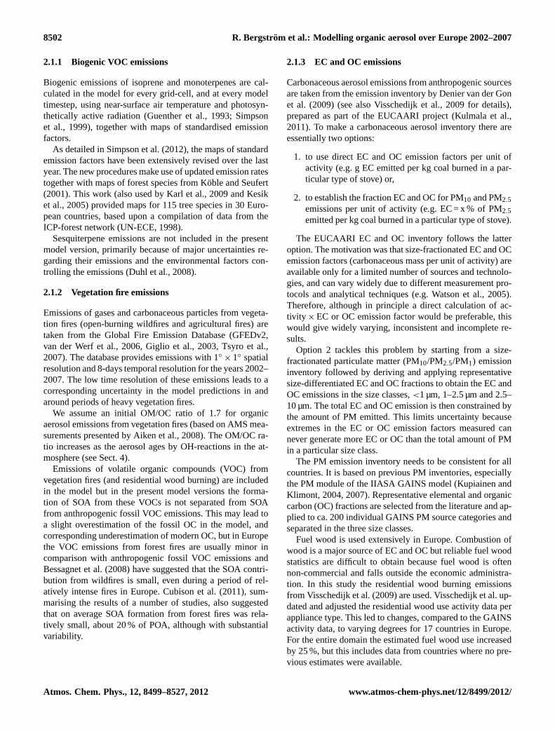
Fig. 1. Emission intensity pattern of OC in PM2.5 overEurope (low to high: blue, green, yellow, orange, red).Unit: tonnes gridcell−1 yr−1.
Another important feature of the new inventory is itsimproved spatial resolution of 1/8◦
× 1/16◦ lon-lat (or∼ 7 km× 7 km) compared to previous inventories. The emis-sions are gridded using especially prepared distributionmaps. Particular attention has been given to the spatial dis-tribution of transport emission and emission due to residen-tial combustion. An example of the emission distribution pat-tern for OCPM2.5 (organic carbon in particles with diameter<2.5 µm) is presented in Fig.1. The emissions are dominatedby transport and residential combustion as can be seen bythe highlighted urban centers, major road network and shiptracks.
Total carbonaceous aerosol emissions in PM2.5 are pre-sented in Table1. Total PM2.5 emissions in Europe amountto ∼3400 ktonnes and about half of the total PM2.5 emissionsin Europe are carbonaceous aerosol, highlighting the impor-tance of this fraction. Elemental carbon emissions are dom-inated by road transport and residential combustion (each∼30 %; Table 1) but for OC residential combustion is clearlythe dominant source, responsible for almost 50 % of the Eu-ropean emissions (Table1).
Particle size distributions of EC and OC for mass showmaxima in the range of 80 to 200 nm, thus being highly rel-evant for long range atmospheric transport. In the presentEMEP PCM model only two size classes are used for the ECand OC emissions, PM-fine (up to 2.5 µm) and PM-coarse(2.5–10 µm), thus the PM1 and PM1−2.5 classes from theemission inventory are combined.
Emissions in the inventory are given in ktonne(C) yr−1.In the model this is converted to OM-emissions using theOM/OC ratios 1.25 for fossil fuel emissions and 1.7 for woodburning emissions, based on data from laboratory and fieldmeasurements (Aiken et al., 2008).
0
5
10
15
20
25
30
35
40
45
50
Jan Feb Mar Apr May Jun Jul Aug Sep Oct Nov Dec
Seasonal variation of OC2.5-emissions
10. Agriculture
9. Waste treatment & disposal
8. Other mobile sources
7. Road transport
6. Solvent use
5. Extract&Distrib of fossil fuels
4. Industrial processes
3. Industrial combustion
2. Residential combution
1. Power generation
SNAP-sectors
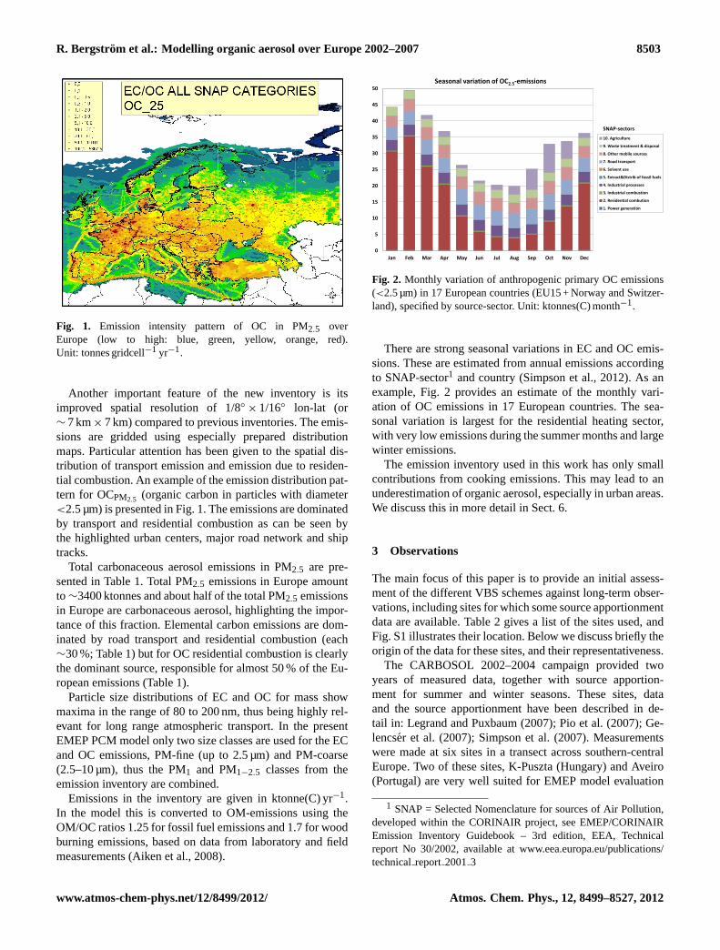
Fig. 2. Monthly variation of anthropogenic primary OC emissions(<2.5 µm) in 17 European countries (EU15 + Norway and Switzer-land), specified by source-sector. Unit: ktonnes(C) month−1.
There are strong seasonal variations in EC and OC emis-sions. These are estimated from annual emissions accordingto SNAP-sector1 and country (Simpson et al., 2012). As anexample, Fig.2 provides an estimate of the monthly vari-ation of OC emissions in 17 European countries. The sea-sonal variation is largest for the residential heating sector,with very low emissions during the summer months and largewinter emissions.
The emission inventory used in this work has only smallcontributions from cooking emissions. This may lead to anunderestimation of organic aerosol, especially in urban areas.We discuss this in more detail in Sect.6.
3 Observations
The main focus of this paper is to provide an initial assess-ment of the different VBS schemes against long-term obser-vations, including sites for which some source apportionmentdata are available. Table2 gives a list of the sites used, andFig. S1 illustrates their location. Below we discuss briefly theorigin of the data for these sites, and their representativeness.
The CARBOSOL 2002–2004 campaign provided twoyears of measured data, together with source apportion-ment for summer and winter seasons. These sites, dataand the source apportionment have been described in de-tail in: Legrand and Puxbaum(2007); Pio et al.(2007); Ge-lencser et al.(2007); Simpson et al.(2007). Measurementswere made at six sites in a transect across southern-centralEurope. Two of these sites, K-Puszta (Hungary) and Aveiro(Portugal) are very well suited for EMEP model evaluation
1 SNAP = Selected Nomenclature for sources of Air Pollution,developed within the CORINAIR project, see EMEP/CORINAIREmission Inventory Guidebook – 3rd edition, EEA, Technicalreport No 30/2002, available atwww.eea.europa.eu/publications/technicalreport20013
www.atmos-chem-phys.net/12/8499/2012/ Atmos. Chem. Phys., 12, 8499–8527, 2012
8504 R. Bergstrom et al.: Modelling organic aerosol over Europe 2002–2007
Table 1.Estimated EC and OC emissions (<2.5 µm) for UNECE Europe in 2005 by source sector (ktonne(C) yr−1).
EC OCSNAP Description kt yr−1 % kt yr−1 %
1. Combustion in energy industries 20 3 11 12. Residential and non-industrial combustion 186 30 395 473. Combustion in manufacturing industry 6 1 9 14. Production processes 36 6 81 105. Extraction and distribution of fossil fuels 4 1 1 06. Solvent use 0 0 0 07. Road transport 201 32 104 128. Other mobile sources and machinery 95 15 71 89. Waste treatment and disposal 37 6 63 710. Agriculture 36 6 112 13
Total excluding international shipping 623 100 848 100
International shipping 124 84
since they are located in rural areas, and at low elevation.We have also made use of data from two of the elevatedsites from the CARBOSOL campaign, Schauinsland (Ger-many) and Puy de Dome (France), since they are usually lo-cated within the planetary boundary layer in summertime,although not usually in winter time. We have excluded theremote Azores and the very high-altitude station Sonnblicksince they are not representative of European boundary layerpollution levels.
Other long-term data-sets consist of the EMEP EC/OCcampaign 2002–2003 (Yttri et al., 2007), and the EMEP PMintensive campaign 2006–2007 (Yttri et al., 2008; Aas et al.,2012). As noted inYttri et al. (2007) most of these sites areestablished EMEP sites, which fulfil the criteria of regionalbackground sites. Penicuik (Scotland) is also a regional back-ground site, although not an EMEP site. Gent (Belgium)and San Pietro Capofiume (Italy) are both urban backgroundsites. Some of the EMEP sites are also quite elevated; we willdiscuss the implications of this while discussing the results inSect.5.
For source apportionment data, we make use of three stud-ies: CARBOSOL as discussed above, the SORGA campaignin and near Oslo in southern Norway (Yttri et al., 2011), andthe Gote-2005 campaign in and near Gothenburg in southernSweden (Szidat et al., 2009). All of these campaigns madeuse of radiocarbon (14C) data as well as of compounds thatcould be used as tracers for wood-burning and primary bio-logical aerosol particles. Further, these source apportionmentstudies were all conducted with different variants of the samemethodology, using Latin-hypercube-sampling to allow for awide range of uncertainties in the relations between tracersand their associated TC components. The Oslo and Gothen-burg sites are urban, which raises some problems when com-paring with results from the EMEP model; this will be ad-dressed where appropriate in Sect.5.
Aerosol mass spectrometry is becoming a very importanttechnique for studying submicron particles (PM1) at hightime-resolution (e.g.Canagaratna et al., 2007). We plan amore extensive comparison with AMS data in a complemen-tary study, here we compare model results to observationsfrom one AMS-campaign, in Switzerland in June 2006 (Lanzet al., 2010), in order to give a first impression of model per-formance at higher time-resolution.
4 VBS experiments
The VBS approach was introduced by Donahue and co-workers (Donahue et al., 2006, 2009), as a practical ap-proach to dealing with the complexity of organics in theatmosphere. The VBS consists of a group of lumped com-pounds with fixed saturation concentrations (C∗, µg m−3),comprising a number of bins separated by one order of mag-nitude each inC∗ at 298 K. Different SOA-forming reactionscan be mapped onto the same set of bins over the range oforganic aerosol mass concentration typical of ambient con-ditions (0.1–100 µg m−3) while maintaining mass balancefor more volatile co-products as well. Aging reactions canbe added easily within the VBS if the kinetics and volatilitydistribution of the products can be measured or estimated.
A number of papers have illustrated the use of VBS-basedmodels in North America (Robinson et al., 2007; Lane et al.,2008a,b; Shrivastava et al., 2008; Murphy and Pandis, 2009),Mexico City (e.g.Dzepina et al., 2009, Hodzic et al., 2010a,Tsimpidi et al., 2010, Li et al., 2011, Shrivastava et al., 2011),and very recently in Europe (Simpson et al., 2009; Foun-toukis et al., 2011), and we build upon this work here.
In the EMEP models for particulate carbonaceous mat-ter (EMEP-PCM) a small four-bin VBS is used for theSOA components (saturation concentrations in the range 1–1000 µg m−3) as inLane et al.(2008b). A larger basis set,
Atmos. Chem. Phys., 12, 8499–8527, 2012 www.atmos-chem-phys.net/12/8499/2012/

R. Bergstrom et al.: Modelling organic aerosol over Europe 2002–2007 8505
Table 2.Measurement sites and campaigns used in this study (see also Fig. S1).
Country Latitude Longitude Alt. (m a.s.l.) Measurements Notes
Schauinsland [DE03] Germany 47.91 7.91 1205 EC, OC, S-A†, PM10 (a), (g)Puy de Dome [FR30] France 45.77 2.95 1450 EC, OC, S-A, PM10 (a), (g)K-puszta [HU02] Hungary 46.97 19.58 125 EC, OC, S-A, PM2.5 (a)Aveiro [AVE] Portugal 40.58 −8.64 47 EC, OC, S-A, PM2.5 (a)Virolahti [FI17] Finland 60.53 27.69 8 EC, OC, PM10 (b)Aspvreten [SE12] Sweden 58.80 17.38 20 EC, OC, PM10 (b)Birkenes [NO01] Norway 58.38 8.25 190 EC, OC, PM10, PM2.5 (2006,2007) (c), (d)Penicuik [GB46] United Kingdom 55.86 −3.21 180 EC, OC, PM10 (b)Kollumerwaard [NL09] the Netherlands 53.33 6.28 0 EC, OC, PM10 (b)Mace Head [IE31] Ireland 53.33 −9.90 25 EC, OC, PM10 (b)Langenbrugge [DE02] Germany 52.80 10.76 74 EC, OC, PM10 (b)Gent [BE05] Belgium 51.05 3.72 0 EC, OC, PM10 (b) (h)Kosetice [CZ03] Czech Republic 49.58 15.08 534 EC, OC, PM10 (b), (c)Stara Lesna [SK04] Slovakia 49.15 20.28 808 EC, OC, PM10 (b)Illmitz [AT02] Austria 47.77 16.77 117 EC, OC, PM10, PM2.5 (S, 2006) (b), (c), (j 2006)Ispra [IT04] Italy 45.80 8.63 209 EC, OC, PM10 (2002-2003), PM2.5 (2006,2007) (b), (c)San Pietro Capofiume [IT10] Italy 44.48 11.33 10 EC, OC, PM10 (b), (h)Braganca [PT01] Portugal 41.82 −6.77 691 EC, OC, PM10 (b)Harwell [GB36] United Kingdom 51.57 −1.32 137 EC, OC, PM10 (S) (c), (i)Melpitz [DE44] Germany 51.53 12.93 87 EC, OC, PM10, PM2.5 (c)Payerne [CH02] Switzerland 46.81 6.94 510 EC, OC, PM2.5, AMS (c), (i)Montelibretti [IT01] Italy 42.10 12.63 48 EC, OC, PM10, PM2.5 (c)Montseny [ES1778] Spain 41.77 2.35 700 EC(S), OC(S), TC(W), PM10 (c)Hurdal [HUR] Norway 60.37 11.07 300 EC, OC, S-A, PM1 (e)Oslo [OSL] Norway 59.93 10.73 77 EC, OC, S-A, PM1 (e), (h)Gothenburg [GOT] Sweden 57.72 11.97 20 EC, OC, S-A, PM10 (W), PM2.5 (S) (f), (h)Rao [SE14] Sweden 57.39 11.91 10 EC, OC, S-A PM2.5 (W) (f)
Notes:† S-A indicates data for source-apportionment, see below; (S) indicates summer, (W) indicates winter; (a) CARBOSOL campaign, July 2002–September 2004, usedweekly filter measurements of EC, OC, cellulose, levoglucosan, and (for seasonally-pooled samples)14C, seeGelencser et al.(2007), Pio et al.(2007); (b) EMEP EC/OCcampaign, 1 July 2002–1 July 2003, 24h filter measurements of EC and OC, once per week, seeYttri et al. (2007); (c) EMEP PM intensive campaign June 2006(S) and 8January–4 February 2007(W), many different measurements were performed in the campaign, seeYttri et al. (2008), Aas et al.(2012). Here we use daily data from filtermeasurements of EC and OC and hourly AMS (OM) data from Payerne for the summer period; (d) For Birkenes filter measurement data for EC and OC in PM10 wereavailable from EMEP for the full years 2002–2004. The data were either weekly measurements or alternatingly 6-days and 24h measurements; (e) SORGA campaign,southern Norway, 19 June–15 July 2006(S) and 1–8 March 2007(W), included filter measurements of EC, OC, sugars, levoglucosan, and14C, (Yttri et al., 2011), here we usethe PM1 data and compare to the model PM2.5 results; (f) Gote-2005 campaign, southern Sweden, 11 Feburary–4 March 2005(W) and 13 June-4 July 2006(S), includedmeasurements of EC, OC, sugars, levoglucosan, and14C, (Szidat et al., 2009); (g) Mountain station; (h) Urban background station; (i) Hourly observation data were available,averaged here to daily means (except for the AMS data, that were averaged to hourly means).
with nine bins, is used for the directly emitted organic aerosolcomponents (of low to intermediate volatility, that is, in par-ticulate as well as gaseous form) from fossil fuel use, res-idential wood combustion and vegetation fires, to cover thegreat range of different volatilities of these species (Robinsonet al., 2007; Shrivastava et al., 2008).
The temperature dependence of the gas-particle partition-ing is taken into account by using the Clausius-Clapeyronequation to calculate the saturation concentrations, alongwith the enthalpy of vaporization,1Hvap. In principle,1Hvap should vary across the VBS bins, with higher valuesfor the lowerC∗ values (Epstein et al., 2010). In this studywe use the1Hvap-values fromRobinson et al.(2007), for thenine-bin VBS used for the primary emissions (values varyfrom 64 kJ mol−1 for the most volatile bin to 112 kJ mol−1
for the least volatile). The VBS-parameterisation of SOAyields from Pathak et al.(2007) used a constanteffective1Hvap= 30 kJ mol−1, for the four-bin VBS. This value wasselected to reproduce the observed temperature dependenceof the smog chamber aerosol yields and accounts for varioustemperature effects on the SOA yields. Here we use thisef-fective1Hvap for the SOA from VOC (similar to e.g.Lane
et al., 2008a,b; Murphy and Pandis, 2009; Farina et al.,2010).
Four versions of the EMEP model have been set up, in-troducing different aspects of the VBS approach in each ver-sion and testing various assumptions about aging reactionsof OA-components in the gas phase. The model versions aresummarised in Table3, and discussed below.
In all model versions, BSOA formation from terpenes isinitiated by gas phase oxidation by O3, OH or NO3 in themodel. For isoprene, only oxidation by OH leads to BSOAformation. As noted in Sect.2.1.1, we only include iso-prene and mono-terpenes among the biogenic species, andnot sesquiterpenes. Initial OM/OC ratios are assumed to be1.7 for BSOA from terpenes and 2.0 for isoprene BSOA(based onChhabra et al., 2010). In the following, we willdenote SOA formed from anthropogenic emissions of VOCfrom fossil sources (“traditional” ASOA) as ASOAV
f . ForASOAV
f from alkanes and alkenes OM/OC = 1.7 is used andfor ASOAV
f from aromatic VOCs the ratio is 2.1 (Chhabraet al., 2010).
It should be stressed that we regard all of these versionsas experiments, in order to demonstrate the importance of
www.atmos-chem-phys.net/12/8499/2012/ Atmos. Chem. Phys., 12, 8499–8527, 2012

8506 R. Bergstrom et al.: Modelling organic aerosol over Europe 2002–2007
Table 3.Summary of the four EMEP model versions used in this study.
Version Volatility S/IVOC/SOA aging Referencesdistributed POA? reactions
NPNA No, POA nonvolatile None Lane et al.(2008a); Tsimpidi et al.(2010)
PAP Yes S/IVOC (4.0×10⁻¹¹ cm3molecule−1s−1) Shrivastava et al.(2008)
PAPA Yes S/IVOC (4.0×10⁻¹¹ cm3molecule−1s−1), Murphy and Pandis(2009); Tsimpidi et al.(2010)ASOAV
f (1.0×10⁻¹¹ cm3molecule−1s−1)
PAA Yes S/IVOC (4.0×10⁻¹¹ cm3molecule−1s−1), Lane et al.(2008b)ASOAV
f & BSOA (4.0×10⁻¹² cm3molecule−1s−1)
the various VBS assumptions, and to assess how far suchapproaches can capture observed levels of OM. Sect.6 willdiscuss some of the limitations of VBS assumptions in par-ticular, and of SOA modelling in general.
4.1 NPNA VBS method
The first model version,NPNA (No Partitioning of primaryemissions andNo Aging reactions included), is based on theSOA scheme ofLane et al.(2008a), for SOA formation fromanthropogenic and biogenic VOC (AVOC and BVOC) (al-thoughLane et al.2008aalso included SOA formation fromsesquiterpenes).
The SOA yields are updated to take into account re-cent findings about higher yields from oxidation of aromaticVOCs (Hildebrandt et al., 2009; Ng et al., 2007a; Tsimpidiet al., 2010). The SOA yields are summarised in Table4.
In the NPNA model version, primary organic aerosolemissions (including wood burning and vegetation fire OMemissions) are assumed non-volatile, taken directly from thecarbonaceous aerosol emission data-sets.
4.2 PAP VBS method
The PAP (Partitioning and atmosphericAging of Primarysemi- and intermediate-volatility OC emissions) model in-troduces three important changes to the treatment of the pri-mary organic aerosol emissions and atmospheric chemistry,following suggestions ofShrivastava et al.(2008):
i. The emitted POA is distributed over different volatili-ties (9-bin VBS, including semi-volatile and intermedi-ate volatility OC, S/IVOC) and partitions between thegas and particulate phases. This allows a large fractionof the POA to evaporate.
ii. The POA emissions are assumed to be accompaniedby emissions of intermediate volatility (IVOC) gases,which are currently not captured in either the POAor the VOC inventories. FollowingShrivastava et al.(2008) we assume that the total emissions of S/IVOCs(including low-volatile POA) amount to 2.5 times thePOA inventory. This means that an IVOC mass of 1.5
times the POA emissions is added to the total emissioninput in the model. We use the same emission split andenthalpies of vaporization as inShrivastava et al.(2008)to calculate how much of this material is condensed atany moment. A large part, 68 %, of the primary S/IVOCemission consists of IVOCs withC∗ ranging from 104
to 106 µg m−3.
iii. The emitted S/IVOCs are allowed to react with OHin the gas phase, with each reaction resulting ina shift of the compound to the next lower volatil-ity bin. The OH-reaction rate used in this study,4.0×10−11 cm3molecule−1s−1, is taken fromRobinsonet al. (2007) and corresponds to the base case inShri-vastava et al.(2008). As in Robinson et al.(2007) andShrivastava et al.(2008), we assume a small mass in-crease (7.5 %) with each aging reaction to account foradded oxygen atoms. In this paper we will use the no-tation SOASI for secondary organic aerosol formed byatmospheric oxidation of the S/IVOC emissions. SOASI
from anthropogenic fossil fuel sources will be denotedASOASI
f .
4.3 PAA VBS method
In thePAA version (Partitioning of primary OA andAgingof All semivolatile OA components in the gas phase) agingreactions for SOA-components in the gas phase are also in-cluded with the same assumption of each reaction leading toa lowering of the volatilities of these species by a factor often and a net mass increase by 7.5 % to account for addedoxygen. The OH-reaction rate for SOA-aging (4.0×10⁻¹²
cm3molecule−1s−1) is assumed to be an order of magnitudelower than for the S/IVOCs (as suggested byLane et al.,2008b).
Lane et al.(2008b) showed that including aging reactionsfor SOA leads to serious overestimation of OC concentra-tions in rural areas in eastern USA. They suggest that al-though aging reactions for SOA components do occur, theeffect may not be a net increase in particle mass since decom-position reactions may compete with substitution reactions.In the polluted Mexico City region, with large primary OA
Atmos. Chem. Phys., 12, 8499–8527, 2012 www.atmos-chem-phys.net/12/8499/2012/
R. Bergstrom et al.: Modelling organic aerosol over Europe 2002–2007 8507
Table 4. Mass yields of the semi-volatile surrogate species, with 298K saturation concentrations of 1, 10, 100 and 1000 µg m−3, for theEMEP model SOA precursors for the high- and low-NOx cases (corresponding to peroxy radical reaction with NO and HO2, respectively).
α-values (mass based stoichiometric yields)
Precursor High-NOx Case Low-NOx Case
1 10 100 1000 1 10 100 1000
Alkanes 0 0.038 0 0 0 0.075 0 0Alkenes 0.001 0.005 0.038 0.15 0.005 0.009 0.060 0.225Aromatics 0.002 0.195 0.3 0.435 0.075 0.3 0.375 0.525Isoprene 0.001 0.023 0.015 0 0.009 0.03 0.015 0Terpenes 0.012 0.122 0.201 0.5 0.107 0.092 0.359 0.608
Notes: yields are based onTsimpidi et al.(2010), and references therein. Alkanes (excluding C2H6), alkenes(excluding C2H4) and aromatics are represented by the surrogates n-butane, propene, o-xylene in the EMEPchemistry.
emissions, even the aging of the primary S/IVOC emissionsin a PAP-like VBS-model may lead to significant overestima-tion of SOA, which was recently shown byShrivastava et al.(2011).
4.4 PAPA VBS method
Murphy and Pandis(2009) include aging reactions for theprimary OA and S/IVOC and anthropogenic SOA but notfor biogenic SOA. In this study we test this assumption inthe PAPA version (Partitioning andAging of Primary OAandAnthropogenic SOA), using the aging rates suggested byMurphy and Pandis(2009), 4.0×10⁻¹¹ cm3molecule−1s−1
for S/IVOC and 1.0×10⁻¹¹ cm3molecule−1s−1 for ASOAVf .
We make the same assumption about additional oxygen massdue to aging reactions in the PAPA model version as in thePAP and PAA versions. This means that the PAPA modelis very similar to the VBS-scheme used byTsimpidi et al.(2010) (Murphy and Pandis2009treated the additional oxy-gen due to aging differently).
5 Results
5.1 Total organic aerosol in PM2.5
Figure 3 shows calculated total organic mass in PM2.5(OMPM2.5) concentrations with the four different model vari-ants (six-year average for the whole period 2002–2007).
In the simplest model version (NPNA), with no aging ofthe aerosol, and the primary OA emissions treated as non-volatile, the calculated OM concentrations are low in largeparts of Europe. The OM distribution reflects the emissioninventory with the highest concentrations in France, Russia,Latvia and a region in Central Europe (the Czech Republic,Slovakia and southern Poland). A few other hotspots withhigh concentrations are also seen; most notably Oslo (Nor-way), Istanbul/Bosphorus Strait, northern Portugal and pointsources in Ukraine.
When the primary emissions are treated in the VBS, andare subject to evaporation and aging reactions (PAP), the pic-ture changes and the concentrations are more homogeneousacross Europe. OM concentrations in the hotspots are de-creased (in spite of the increase in total POA emitted in thePAP model), due to evaporation of part of the POA emis-sions. The levels further away from the main emission ar-eas are increased due to the aging reactions that decrease thevolatility of the semi-volatile OC. Eastern and Central Eu-rope, as well as parts of France, the Po Valley and the Oslo re-gion, have the highest OM concentrations (above 3 µg m−3).
Adding aging reactions also for the SOA (PAPA and PAAmodels) increases the calculated OM concentrations further.In the model version including aging of BSOA (PAA) themodel OM is above 3 µg m−3 in large parts of Europe (themain exceptions are the British Isles and the northern part ofScandinavia and Russia that have low concentrations of or-ganic aerosol). OM concentrations above the Mediterraneanand Black Seas are elevated in the PAPA and PAA models.This accumulation over the sea areas is likely due to fairlyhigh concentrations of OH in these regions, leading to highoxidation rates for the semi-volatile OA components in thegas phase, and little precipitation, which means small depo-sition losses.
The realism of these concentration levels is consideredin relation to measurements, and in more general terms, inSect.5.4and Sect.6.
5.2 Contributions from different sources to organicaerosol in Europe
In Fig. 4 (and Figs. S2–S4) the calculated relative contribu-tions to OMPM2.5 from different sources are compared. Al-though it is not clear which model version can be consideredmost realistic we choose to show results for the PAA ver-sion here, since it gives the highest modelled OMPM2.5 andincludes more atmospheric processing of the OA than theother versions (results for the other versions are given in the
www.atmos-chem-phys.net/12/8499/2012/ Atmos. Chem. Phys., 12, 8499–8527, 2012

8508 R. Bergstrom et al.: Modelling organic aerosol over Europe 2002–2007
Fig. 3. Total Organic Matter in PM2.5 (OMPM2.5). 6-yr average concentration (for the period 2002–2007) calculated with the EMEP-PCM
model. Comparison between four different model versions (see text). Unit: µg m−3.
Supplement, and in more detail, for selected sites, in Fig.5a,b and S5–S6).
Several different sources contribute significantly to themodelled OMPM2.5. Biogenic SOA is an important compo-nent; in parts of Finland and Spain and the Mediterranean re-gion the BSOA contribution to OMPM2.5 is above 30 % in thePAA version, which has the highest BSOA levels, becauseof the aging reactions of semi-volatile biogenic species. Inmodel versions that do not include atmospheric aging ofBSOA the importance of this source is much lower (below20 % in most of Europe, see Figs. S2–S4).
The importance of anthropogenic SOA from fossil sources(ASOA = ASOAV
f + ASOASIf ) is very sensitive to assump-
tions regarding the aging reactions in the atmosphere. In thesimplest model version (NPNA, Fig. S2), which only in-cludes traditional ASOA from AVOC and no atmosphericaging, the contribution to OMPM2.5 is below 10 % in all ofEurope. All other model versions include the formation ofASOASI
f from the primary S/IVOC emissions and this givesmore than 10 % ASOA in most of Europe; only the north-ern part has less ASOA. When atmospheric aging of (tra-ditional) ASOAV
f is also included (PAA and PAPA models)
Atmos. Chem. Phys., 12, 8499–8527, 2012 www.atmos-chem-phys.net/12/8499/2012/

R. Bergstrom et al.: Modelling organic aerosol over Europe 2002–2007 8509
Fig. 4.Calculated relative contribution to organic matter in PM2.5 (OMPM2.5) from different sources, using the PAA model version. Fractionof OMPM2.5 from (a) anthropogenic SOA (from AVOC and fossil fuel S/IVOC, i.e., ASOAV
f + ASOASIf ), (b) fossil fuel primary organic
aerosol (POA),(c) biogenic SOA (from BVOC),(d) background organic aerosol (from sources not explicitly included in the model),(e)residential wood combustion (primary + SOASI), (f) vegetation fires (primary + SOASI). Average for the 6-yr period 2002–2007.
www.atmos-chem-phys.net/12/8499/2012/ Atmos. Chem. Phys., 12, 8499–8527, 2012

8510 R. Bergstrom et al.: Modelling organic aerosol over Europe 2002–2007
Fig. 5.Modelled contribution from different sources to OCPM10, at sites from the EMEP EC/OC campaign 2002-2003 and the CARBOSOLproject, arranged from north to south. Long-term averages for the different model versions (NPNA, PAP, PAPA and PAA, see text). For mostsites the data are averages for the period July 2002–June 2003 but for the two stations Schauinsland and Puy de Dome (from the CARBOSOLproject), the averages are for October 2002–September 2004. Colours/Notation, Dark grey: primary OA in PM2.5−10 (coarse mode); Lightgrey: primary OA in PM2.5; medium blue: anthropogenic SOA from aged S/IVOC emissions; dark blue: anthropogenic SOA from VOC;dark brown: primary OA from Residential Wood Combustion (RWC); Light brown: aged OA from RWC S/IVOC emissions; orange: primaryOA from vegetation fires (open-burning wildfires and agricultural fires); light orange: aged OA from vegetation fires; dark green: biogenicSOA from terpenes and isoprene; light green: background OA, from sources not included in the model.
the importance of ASOA is further enhanced. In the PAPAmodel, with a high rate for the ASOAVf aging, the modelASOA fraction of the total OMPM2.5 is 40–50 % over mostof the Mediterranean Sea and in the Po Valley. This is dueto high OH-concentrations, low deposition over the sea and(in some parts) high VOC emissions; in such conditions thePAPA model gives a very high SOA yield for emitted aro-matic VOCs (sometimes approaching 100 %, at least duringsummer), much larger than those found in smog-chamberstudies byNg et al.(2007a). This issue is discussed furtherin Sect.6.
For the period 2002–2007, vegetation fires seem to be amajor source of OMPM2.5 in some parts of Europe, most no-tably Russia and eastern Europe and Portugal and westernSpain. In these regions more than 10 % of the long-term aver-age OMPM2.5 may be due to vegetation fire emissions. How-ever, if the emissions are treated as nonvolatile and not ag-
ing in the atmosphere the impacts are much more local (seeFig. S2).
In the PAA-model the primary (fresh) fossil fuel OA con-tribution to OMPM2.5 is relatively low in most of Europe,ranging from 2–10 %, and even lower in parts of southern Eu-rope (due to evaporation and rapid loss of POA compoundsby oxidation). In some emission hot-spots (e.g. Paris andMoscow) the contribution is 10–20 %.
If the primary emissions are treated as nonvolatile (NPNA-version, Fig. S2) the fresh POA fraction of the total OA ismuch higher; in this version there is no evaporation of theemitted POA in the emission regions, which leads to highcontributions in the major source areas.
We find relatively large contributions of residential woodburning to OMPM2.5, above 10 % in large parts of Europe inall model versions.
In Fig. 5a, b (and S5–S6) the contribution of the differentsources to OC are shown in more detail for different sites in
Atmos. Chem. Phys., 12, 8499–8527, 2012 www.atmos-chem-phys.net/12/8499/2012/
R. Bergstrom et al.: Modelling organic aerosol over Europe 2002–2007 8511
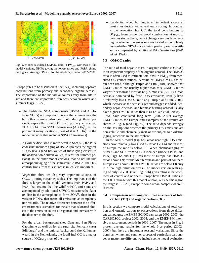
Fig. 6. Model calculated OM/OC ratio in PM2.5 with two of themodel versions, NPNA giving the lowest ratios and PAPA givingthe highest. Average OM/OC for the whole 6-yr period 2002–2007.
Europe (sites to be discussed in Sect. 5.4), including separatecontributions from primary and secondary organic aerosol.The importance of the individual sources vary from site tosite and there are important differences between winter andsummer (Figs. S5–S6):
– The traditional SOA components (BSOA and ASOAfrom VOCs) are important during the summer monthsbut other sources also contribute during these pe-riods, especially fossil OC from primary emissions,POA + SOA from S/IVOC-emissions (ASOASI
f ), is im-portant at many locations (most of it is ASOASI
f in themodel versions that includes S/IVOC emissions).
– As will be discussed in more detail in Sect.5.5, the PAAcode (that includes aging of BSOA) predicts the highestBSOA levels (and has values of these lying closest tothe observation-derived values, at least for summer pe-riods). In the other model versions, that do not includeatmospheric aging of the semi-volatile BSOA, the OC-contributions from this source is much less important.
– Vegetation fires are also very important sources ofOCPM10 during certain episodes. The importance of thefires is larger in the model versions PAP, PAPA andPAA, that assume that the wildfire POA emissions areaccompanied by additional S/IVOC emissions that lateroxidise in the atmosphere to form SOASI, than in theversion NPNA, that treats all emissions as completelynon-volatile. The relative difference between the differ-ent treatments is smallest for the site that is located clos-est to the emission source (Braganca) and increase withthe distance to the fires.
– For the urban background sites Gent and San PietroCapofiume as well as for the rural site Penicuik (nearEdinburgh) and the regional background site Kollumer-waard in the Netherlands, the fossil fuel OC is a majorsource of OCPM10 most of the time.
– Residential wood burning is an important source atmost sites during winter and early spring. In contrastto the vegetation fire OC, the total contributions toOCPM10 from residential wood combustion, at most ofthe sites studied here, do not change very much depend-ing on whether the emissions are treated as completelynon-volatile (NPNA) or as being partially semi-volatileand accompanied by additional IVOC-emissions (PAP,PAPA, PAA).
5.3 OM/OC ratios
The ratio of total organic mass to organic carbon (OM/OC)is an important property of the organic aerosol. The OM/OCratio is often used to estimate total OM in PM2.5 from mea-sured OC concentrations. A value of OM/OC = 1.4 has of-ten been used, althoughTurpin and Lim(2001) showed thatOM/OC ratios are usually higher than this. OM/OC ratiosvary with season and location (e.g.Simon et al., 2011). Urbanaerosols, dominated by fresh POA emissions, usually havea relatively low OM/OC ratio (e.g.Turpin and Lim, 2001),which increase as the aerosol ages and oxygen is added. Sec-ondary organic aerosol and biomass burning aerosol usuallyhave higher OM/OC ratios than POA (Aiken et al., 2008).
We have calculated long term (2002–2007) averageOM/OC ratios for Europe and examples of the results areshown in Fig.6 (and Fig. S7). The ratio depends stronglyon the assumptions whether the primary OA emissions arenon-volatile and chemically inert or are subject to oxidation(aging) reactions in the atmosphere.
In the NPNA model (Fig.6a), areas near high POA emis-sions have relatively low OM/OC ratios (< 1.6) and in mostof Europe the ratio is below 1.9. When chemical aging ofS/IVOC and SOA from VOC is included (models PAPA andPAA, Figs. 6b and Fig. S7d) most of Europe has OM/OCratios above 1.9; for the Mediterranean and parts of southernEurope even above 2.0; the OM/OC ratios are below 1.8 onlyin a few high emission areas. The model version with ag-ing of only S/IVOC (PAP, Fig. S7b) gives ratios in between;most of central and northern Europe have OM/OC ratios inthe 1.8–1.9 range with this model version, outside this regionthe range is 1.9–2.0, except in some urban hotspots where itis lower.
5.4 Comparison with long-term measurements of totalcarbon (TC) and organic carbon (OC)
In this section we compare model calculations of total car-bon and organic carbon to observations from three differ-ent campaigns, the EMEP EC/OC campaign 2002–2003, theCARBOSOL project 2002–2004, and the EMEP PM inten-sive measurement periods in 2006–2007. The maps in Fig.3present average results for the whole 6-yr period (2002–2007), but there are important seasonal variations. Since thedominant winter and summer sources of particulate carbona-ceous matter are different we include some model evaluation
www.atmos-chem-phys.net/12/8499/2012/ Atmos. Chem. Phys., 12, 8499–8527, 2012

8512 R. Bergstrom et al.: Modelling organic aerosol over Europe 2002–2007
Fig. 7. Observed and modelled TCPM10 during the summer half-year period (May–October) at different European sites from theCARBOSOL (2002–2004) and EMEP EC/OC (2002–2003) cam-paigns. The leftmost bars show observed average concentrations(black for stations located at less than 600 m altitude, light gray forsites above 1000 m and medium gray for stations at 600–1000 mheight) and the following four bars the corresponding model con-centrations with the four different model versions (NPNA, PAP,PAPA and PAA). The colours of the model bars illustrate the corre-lation coefficients, see legend. Some stations are moved for clarity,location indicated with arrows. Note that number of samples variesbetween stations (N = 13 for CZ03,N ≥ 22 for other sites) – seeTable S1 for details and results from other campaigns.
data split into summer and winter half-years (here the sum-mer period is defined as the months May–October).
The results for total carbon in PM10 samples (TCPM10)are illustrated in Figs.7 (summer) and8 (winter) and sum-marised in Table S1 and Figs. S8–S9. Figs. S10–S11 and Ta-ble S2 contain results for TC in PM2.5 (TCPM2.5).
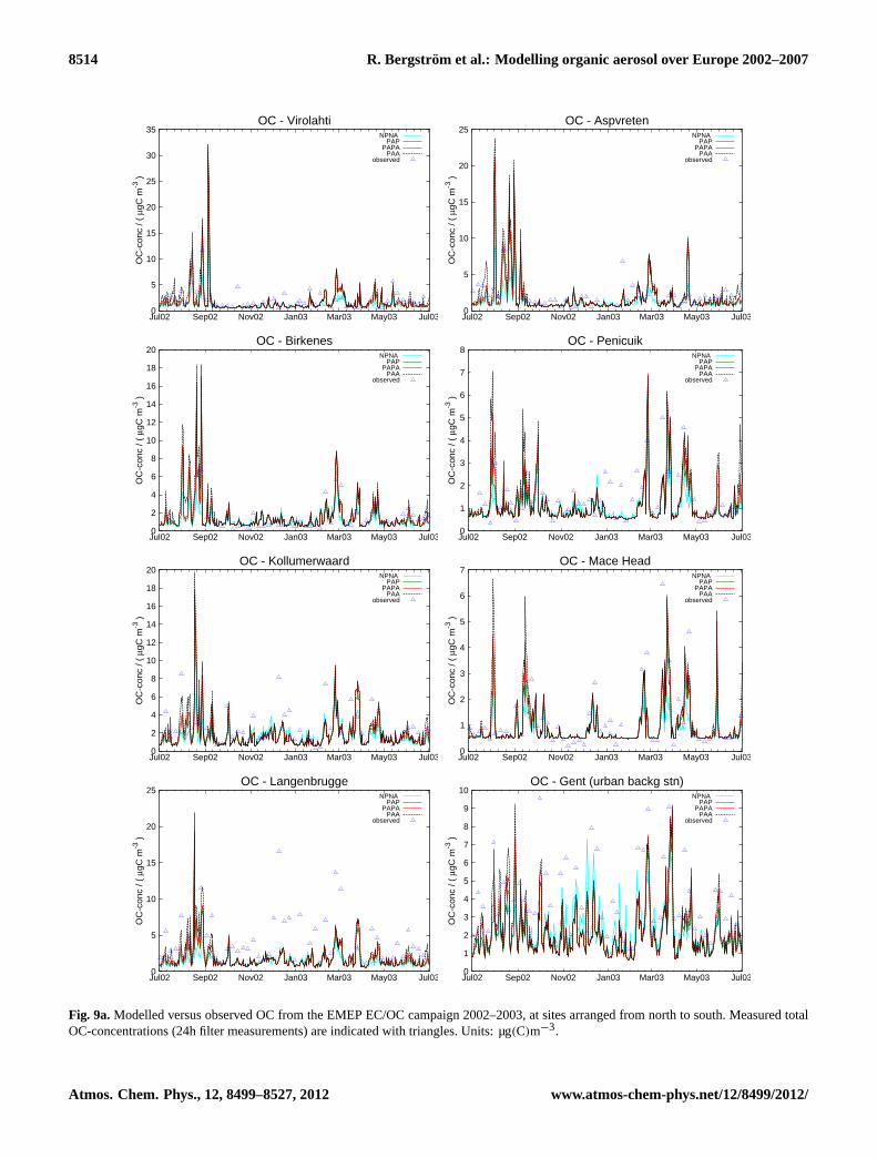
Since a major part of the total carbon in particulate matteris organic carbon the model results for OC are usually simi-lar to those for TC. For organic carbon the modelled seasonalvariations are illustrated in time series plots in Figs.9a, b, atdifferent locations in Europe, together with measured con-centrations from the EMEP EC/OC (2002–2003) and CAR-BOSOL (2002–2004) campaigns. A detailed comparison ofthe OCPM10 model results to observations, including data alsofrom the shorter EMEP intensive measurements periods in2006 and 2007, is given in Table S3 and results for OCPM2.5
in Table S4.Comparing the different model versions there is a clear
increase in TCPM10 (and OCPM10) from the simplest model(NPNA) to the model that includes most aging reactions(PAA), although the increase is more marked in summer-time. Model results for summer are generally much betterthan for winter, e.g., the mean absolute error (MAE) of themodel results (based on data from all stations in Table S1)range from 1.4 (PAA)–1.8 (NPNA) µg(C)m−3 (43–56 %) for
Fig. 8.Observed and modelled TCPM10 during the winter half-yearperiod (November–April) at different European sites from the CAR-BOSOL (2002–2004) and EMEP EC/OC (2002–2003) campaigns.Details/Notation see Fig.7.
summer and about 2.6 µg(C)m−3 (66 %, for all model ver-sions) in winter. Correlation coefficients are also higher forsummer, ranging from 0.66 (NPNA) to 0.58 (PAP), than forwinter. Results for OCPM10 are similar (see Table S3).
It should be noted that model performance varies greatlybetween different sites, partly reflecting their location andrepresentativeness. For the Nordic sites, correlation coeffi-cients for all the model versions are in the range 0.7–0.8 (forthe full-year). The Swedish and Finnish sites (Aspvreten andVirolahti) have very high correlation for summer (r ∼ 0.9)but much lower for the winter half-year months (ca. 0.3–0.4);the mean model bias is low at both sites during both winterand summer when the PAA model is used. For the Norwe-gian station Birkenes correlation coefficients are relativelyhigh both during winter and summer but all model versionsoverestimate TC and OC during winter. At most other (non-mountain) sites the model underestimates winter concentra-tions a lot. Outside the northern part of Europe some sitesare very poorly described by the model, especially the urban-influenced Ispra and San Pietro Capofiume, in Italy, and Bra-ganca in Portugal. For Ispra (summer and winter) and Bra-ganca (winter) the correlation between model and measuredTCPM10 is close to zero and winter time OCPM10 concentra-tions are underestimated by a factor of 6.
The deterioration of model results with increased aging(i.e. more SOA) at the urban-influenced sites in the south isprobably a signal that the observations are influenced moreby primary emissions than the model suggests. Adding fur-ther SOA, which responds very differently to dispersion andchemical processing, only makes such a comparison worse.
The time-series plots of OCPM10 in Fig. 9a, b illustratethe day-to-day variation in the modelled OC-concentrations.Many of the largest peaks seen at many sites in northern andcentral Europe (and at Braganca), in the late summer 2002,are totally dominated by contributions from vegetation fires.
Atmos. Chem. Phys., 12, 8499–8527, 2012 www.atmos-chem-phys.net/12/8499/2012/

R. Bergstrom et al.: Modelling organic aerosol over Europe 2002–2007 8513
Observations at some sites that are occasionally subjectto very clean air, such as the near coastal sites Mace Head(Ireland) and Birkenes (Norway), Aspvreten (Sweden), Kol-lumerwaard (the Netherlands) and Penicuik (the UK), indi-cate that the background OC concentration used in the model(0.5 µg(C)m−3) is too high, at least during winter. About10 % of the winter measurements and about 3 % of the sum-mer measurements of TCPM10 are lower than 0.5 µg(C)m−3
(see Fig.9a, b, and S8–S9).The high-elevation sites are also interesting. In Figs.7
and 8, high-elevation sites are indicated by light grey ormedium grey bars for the observations, referring to sites atgreater than 1000 m or 600 m respectively. The 600 m thresh-old was chosen somewhat arbitraily, but for example avoidslabelling sites such as Kosetice (534 m a.s.l.) as a mountain-site. Rather this site is located in agricultural countrysideof the Czech-Moravian Highlands. One would expect themodel’s surface concentrations (those we use here) to over-predict concentrations at elevated stations. For the wintermonths this is clearly seen in the time series plots for Puy deDome and Schainsland, in Fig.9b; measured concentrationsare often very low during winter, indicating that the sites lieabove the polluted planetary boundary layer during these pe-riods. However, for summer conditions these sites are muchmore similar to other central European sites and at least themodel version PAA gives TCPM10 and OCPM10 in fair agree-ment with the observed concentrations. Figure7 shows thatthe correlation coefficients increase substantially in summer-time when SOA formation by aging is included in the modelat the high-altitude sites (those indicated with light or dark-gray bars for the observations), presumably a signal that SOAformation drives particulate carbon variation in these loca-tions.
There is much less data available for TCPM2.5 (Fig-ures S10–S11, and Table S2) and OCPM2.5 (Table S4) than forTCPM10 and OCPM10. The conclusions from comparisons ofmeasured and modelled TC and OC concentrations in PM2.5are similar to those for PM10. Model results for summer aremuch better than for winter and there is a tendency that thePAA model gives summer concentrations in slightly betteragreement with observations than the other model versionsdo.
For the Italian sites (Ispra and Montelibretti) the dif-ferences between summer and winter results for TCPM2.5
are huge. The PAA model gives reasonably good resultsfor both sites for June 2006 (13 and 29 % underestima-tion and correlation coefficients of 0.61 and 0.69, respec-tively). For the winter period (January–February 2007) theobserved TCPM2.5 of Ispra and Montelibretti were very high(ca. 20 µg(C)m−3) and the PAA model results are an order ofmagnitude lower (the model TCPM2.5 for the summer periodare actually much higher than for the winter period). Disper-sion problems could explain some of the wintertime under-prediction, but comparisons for other pollutants (e.g. NO2,not shown) at these sites are in much better agreement with
observations than we find here for TC. Consistent with otherstudies (Simpson et al., 2007; Genberg et al., 2011; Deniervan der Gon et al., 2012), this points to major problems inthe emission inventory (likely the residential wood burningcomponent) for winter emissions, at least in the areas aroundthese sites.
5.5 Source apportionment studies
Since the emission input is known by source sector, themodel results can be compared to source apportionment(S-A) studies that give information about the relative contri-butions from different sources to PCM. This may give furtherindications of the performance of the SOA modules and/orshortcomings of the emission input.
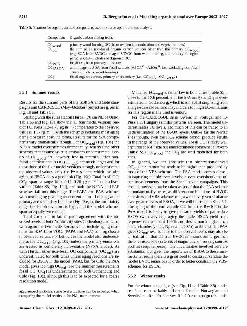
Here we compare model results to three S-A studies whichhave been analysed with essentially the same methodology:the 2-yr CARBOSOL campaign at sites in central Europe(Gelencser et al., 2007), the SORGA campaign in the Osloregion in southern Norway (Yttri et al., 2011), and the Gote-2005 campaign in and close to Gothenburg in southern Swe-den (Szidat et al., 2009). The different studies have split themeasured OC and EC into somewhat different components.Table5 summarises the notation used.
These components and their derivation have been dis-cussed in the three source apportionment studies, most re-cently by Yttri et al. (2011). Some differences exist in thedata available from each study, and in the ratios chosento translate measurements of the tracer to associated OCamounts, but all used the same basic statistical approach ini-tiated in Gelencser et al.(2007). Instead of just providingone estimate for the relative contribution of different sourcesto total carbon, this S-A approach recognises uncertaintiesin the observed data themselves, and in the relationshipsbetween tracers and associated OC. Making use of Latin-hypercube-sampling (e.g.McKay et al., 1979) to explore thenumerous possible uncertain relationships, a statistical dis-tribution of possible solutions was obtained. We make useof the results as expressed through the percentiles (e.g. 5th,50th, 95th) of these solutions.
Concerning the SORGA and Gote urban sites (Oslo andGothenburg), it should be noted that in principle the modelresolution is not well suited for urban measurements. Al-though these cities are relatively small (ca. 0.5 million inhab-itants), some underestimation of especially the primary emis-sion components in wintertime should be expected. For ex-ample,Szidat et al.(2009) found that TC in central Gothen-burg in wintertime was about 1 µg m−3 larger than at thenearby rural site (3 µg m−3 versus 1.8 µg m−3). It is how-ever interesting to compare the results for the two Scandina-vian campaigns2: the Oslo and Gothenburg regions are onlyabout 300 km apart and the cities are also of similar sizes.
2The S-A data from the SORGA measurements in Norway arefrom PM1 measurements. The model results are for PM2.5. Most ofthe PM2.5 mass is expected to be found in PM1 but, especially for
www.atmos-chem-phys.net/12/8499/2012/ Atmos. Chem. Phys., 12, 8499–8527, 2012
8514 R. Bergstrom et al.: Modelling organic aerosol over Europe 2002–2007
0
5
10
15
20
25
30
35
Jul02 Sep02 Nov02 Jan03 Mar03 May03 Jul03
OC
-con
c / (
μgC
m-3
)
OC - VirolahtiNPNA
PAPPAPA
PAAobserved
0
5
10
15
20
25
Jul02 Sep02 Nov02 Jan03 Mar03 May03 Jul03
OC
-con
c / (
μgC
m-3
)
OC - AspvretenNPNA
PAPPAPA
PAAobserved
0
2
4
6
8
10
12
14
16
18
20
Jul02 Sep02 Nov02 Jan03 Mar03 May03 Jul03
OC
-con
c / (
μgC
m-3
)
OC - BirkenesNPNA
PAPPAPA
PAAobserved
0
1
2
3
4
5
6
7
8
Jul02 Sep02 Nov02 Jan03 Mar03 May03 Jul03
OC
-con
c / (
μgC
m-3
)
OC - PenicuikNPNA
PAPPAPA
PAAobserved
0
2
4
6
8
10
12
14
16
18
20
Jul02 Sep02 Nov02 Jan03 Mar03 May03 Jul03
OC
-con
c / (
μgC
m-3
)
OC - KollumerwaardNPNA
PAPPAPA
PAAobserved
0
1
2
3
4
5
6
7
Jul02 Sep02 Nov02 Jan03 Mar03 May03 Jul03
OC
-con
c / (
μgC
m-3
)
OC - Mace HeadNPNA
PAPPAPA
PAAobserved
0
5
10
15
20
25
Jul02 Sep02 Nov02 Jan03 Mar03 May03 Jul03
OC
-con
c / (
μgC
m-3
)
OC - LangenbruggeNPNA
PAPPAPA
PAAobserved
0
1
2
3
4
5
6
7
8
9
10
Jul02 Sep02 Nov02 Jan03 Mar03 May03 Jul03
OC
-con
c / (
μgC
m-3
)
OC - Gent (urban backg stn)NPNA
PAPPAPA
PAAobserved
Fig. 9a.Modelled versus observed OC from the EMEP EC/OC campaign 2002–2003, at sites arranged from north to south. Measured totalOC-concentrations (24h filter measurements) are indicated with triangles. Units: µg(C)m−3.
Atmos. Chem. Phys., 12, 8499–8527, 2012 www.atmos-chem-phys.net/12/8499/2012/

R. Bergstrom et al.: Modelling organic aerosol over Europe 2002–2007 8515
0
5
10
15
20
25
Jul02 Sep02 Nov02 Jan03 Mar03 May03 Jul03
OC
-con
c / (
μgC
m-3
)
OC - KoseticeNPNA
PAPPAPA
PAAobserved
0
5
10
15
20
25
Jul02 Sep02 Nov02 Jan03 Mar03 May03 Jul03
OC
-con
c / (
μgC
m-3
)
OC - Stara LesnaNPNA
PAPPAPA
PAAobserved
0
1
2
3
4
5
6
7
8
9
10
Oct02 Jan03 Apr03 Jul03 Oct03 Jan04 Apr04 Jul04
OC
-con
c / (
μgC
m-3
)
OC - Schauinsland (CARBOSOL, mountain stn)NPNA
PAPPAPA
PAAobserved
0
5
10
15
20
25
Jul02 Sep02 Nov02 Jan03 Mar03 May03 Jul03
OC
-con
c / (
μgC
m-3
)
OC - IllmitzNPNA
PAPPAPA
PAAobserved
0
5
10
15
20
25
30
35
40
Jul02 Sep02 Nov02 Jan03 Mar03 May03 Jul03
OC
-con
c / (
μgC
m-3
)
OC - IspraNPNA
PAPPAPA
PAAobserved
0
2
4
6
8
10
12
Oct02 Jan03 Apr03 Jul03 Oct03 Jan04 Apr04 Jul04
OC
-con
c / (
μgC
m-3
)
OC - Puy de Dome (CARBOSOL, mountain stn)NPNA
PAPPAPA
PAAobserved
0
2
4
6
8
10
12
14
16
18
Jul02 Sep02 Nov02 Jan03 Mar03 May03 Jul03
OC
-con
c / (
μgC
m-3
)
OC - San Pietro Capofiume (urban backg stn)NPNA
PAPPAPA
PAAobserved
0
5
10
15
20
25
30
35
Jul02 Sep02 Nov02 Jan03 Mar03 May03 Jul03
OC
-con
c / (
μgC
m-3
)
OC - BragancaNPNA
PAPPAPA
PAAobserved
Fig. 9b. For Schauinsland and Puy de Dome observation data (indicated by squares) are weekly filter data from the CARBOSOL project,2002–2004. Note that both these sites are mountain sites and often above the planetary boundary layer during winter.
www.atmos-chem-phys.net/12/8499/2012/ Atmos. Chem. Phys., 12, 8499–8527, 2012
8516 R. Bergstrom et al.: Modelling organic aerosol over Europe 2002–2007
Table 5.Notation for organic aerosol components used in source-apportionment analysis.
Component Organic carbon arising from:
OCwood primary wood-burning OC (from residential combustion and vegetation fires)OConf the sum of all non-fossil organic carbon sources other than the primary OCwood,
(e.g. SOA from BVOC and aged S/IVOC from wood-burning, and primary biologicalparticles); also includes background OC.
OCPOA fossil OC, from primary emissionsOCfASOA anthropogenic SOA from fossil sources (ASOAV
f +ASOASIf , i.e., excluding non-fossil
sources, such as, wood-burning)OCf fossil organic carbon, primary or secondary (i.e., OCPOA +OCfASOA)
5.5.1 Summer results
Results for the summer parts of the SORGA and Gote cam-paigns and CARBOSOL (May–October) project are given inFig. 10and Table S5.
Starting with the rural station Hurdal (70 km NE of Oslo),Table S5 and Fig.10a show that all four model versions pre-dict TC levels (1.2–1.78 µg m−3) comparable to the observedvalue of 1.67µg m−3, with the schemes including most agingbeing closest in absolute terms. Results for the S-A compo-nents vary dramatically though. For OCwood (Fig. 10b) theNPNA model overestimates dramatically, whereas the otherschemes that assume volatile emissions underestimate. Lev-els of OCwood are, however, low in summer. Other non-fossil contributions to OC (OConf) are much larger and forthese three of the four model versions strongly underestimatethe observed values, only the PAA scheme which includesaging of BSOA does a good job (Fig.10c). Total fossil OC;OCf, spans a range from 0.11–0.26 µg m−3 in the obser-vations (Table S5, Fig.10d), and both the NPNA and PAPschemes fall into this range. The PAPA and PAA schemeswith more aging give higher concentrations. Looking at theprimary and secondary fractions (Fig.10e, f), the uncertaintyrange for the observations is huge, and the model schemesspan an equally wide range.
Total Carbon is in fair to good agreement with the ob-served levels at both Nordic city sites Gothenburg and Oslo,with again the two model versions that include aging reac-tions for SOA from VOCs (PAPA and PAA) coming closestto observed values. For both cities the model also underesti-mates the OCwood (Fig. 10b) unless the primary emissionsare treated as completely non-volatile (NPNA model). Aswith Hurdal, other non-fossil OC components (OConf) areunderestimated for both cities unless aging reactions are in-cluded for BSOA in the model (PAA), but for Oslo the PAAmodel gives too high OConf. For the summer measurementsfossil OC (OCf) is underestimated in both Gothenburg andOslo (Fig.10d), although this is to be expected for a coarseresolution model.
aged aerosol particles, some overestimation can be expected whencomparing the model results to the PM1 measurements.
Modelled ECwood is rather low in both cities (Table S5) ,close to the 10th percentile of the S-A analysis. ECf is over-estimated in Gothenburg, which is somewhat surprising froma large-scale model, and may indicate too high EC-emissionsfor this region in the used inventory.
For the CARBOSOL sites (Aveiro in Portugal and K-Puszta in Hungary) similar patterns are seen. The model un-derestimates TC levels, and much of this can be traced to anunderestimation of the BSOA levels. Unlike for the Nordicsites though, even the PAA scheme cannot produce resultsin the range of the observed values. Fossil OC is fairly wellcaptured at K-Puszta but underestimated somewhat at Aveiro(Table S5). ECwood and ECf are well modelled for bothsites.
In general, we can conclude that observation-derivedOConf in summertime tends to be higher than produced bymost of the VBS schemes. The PAA model comes closestto capturing the observed levels; it even overshoots the ur-ban measurements from the Scandinavian campaigns. Thisshould, however, not be taken as proof that the PAA schemeis fundamentally better, as different combinations of BVOCemissions and VBS schemes might well have given similar oreven greater levels of BSOA, as we will illustrate in Sect.5.7.The aging of the semi-volatile OC from the BVOCs in thePAA model is likely to give too large yields of particulateBSOA (with very high aging the model BSOA yield fromterpenes can be about 100 % and this is much higher thansmog-chamber yields,Ng et al., 2007b) so the fact that PAAgives OConf results close to the observed levels may also bean indication that the true BVOC emissions are larger thanthe ones used here (in terms of magnitude, or missing sourcessuch as sesquiterpenes). The uncertainties involved here aresubstantial, but given the importance of BSOA to these sum-mertime results there is a great need to constrain/validate themodel BVOC emissions in order to better constrain the VBS-schemes for BSOA.
5.5.2 Winter results
For the winter campaigns (see Fig.11 and Table S6) modelresults are remarkably different for the Norwegian andSwedish studies. For the Swedish Gote campaign the model
Atmos. Chem. Phys., 12, 8499–8527, 2012 www.atmos-chem-phys.net/12/8499/2012/

R. Bergstrom et al.: Modelling organic aerosol over Europe 2002–2007 8517
Fig. 10.Source apportionment studies during summer periods (May–October). Comparison of model results to observation-derived values fordifferent source categories of organic carbon and for total carbon (units µg(C)m−3). The observed values for the different source categoriesare based on a statistical approach (Latin-hypercube sampling) and given as 10–90th percentiles (SORGA and Gote campaigns: NO and SEstations) or 5–95th percentiles (CARBOSOL campaign: HU and PT stations). Further details, see text and Table S5.
underestimates OCwood in Gothenburg but does a good jobfor OConf. Fossil OC and EC are underestimated at the ur-ban station (as expected). The ECwood is well modelled incontrast to the underestimation of OCwood. The model re-sults for the rural background station Rao, outside Gothen-burg, are fairly good for TC (underestimated by ca 20 %) butthe individual components are not so well reproduced, withlarge underestimations of OCwood and OCf and a too highestimate of OConf.
The model results for the Norwegian SORGA campaignare very different and do not agree well with the winter datafrom this campaign. Both the wood burning and other non-fossil contributions are greatly overestimated. At the ruralstation Hurdal the total fossil OC contribution is in goodagreement with the S-A analysis but the fraction of ASOA isgreatly underestimated and the primary OA is overestimated.TC is strongly overestimated even for Oslo where an under-
estimation would be expected with the coarse model resolu-tion used.
The combined results from the SORGA and Gote cam-paigns point to a too high contribution from background OCin the model during winter. Of the four sites only Gothen-burg has OConf concentrations close to or above the modelbackground OC of 0.5 µg(C)m−3. This is consistent with theresults discussed in Sect.5.4.
Wintertime (November–April) OCwood at the CAR-BOSOL sites are underestimated by more than a factor often. Similar results were found bySimpson et al.(2007).That study showed that much higher emissions from wood-burning were required in order to explain the observed lev-oglucosan levels, and accounting for this would also explainalmost all of the discrepancy between modelled and observedTC.
www.atmos-chem-phys.net/12/8499/2012/ Atmos. Chem. Phys., 12, 8499–8527, 2012
8518 R. Bergstrom et al.: Modelling organic aerosol over Europe 2002–2007
For Aveiro fossil OC is also severely underestimated com-pared to the measurements, much more so than inSimpsonet al.2007, presumably as a result of the different emissioninventories in use. Results for K-Puszta are only marginallybetter, fossil OC is underestimated by a factor of five.
5.6 Residential wood burning emissions
Residential burning of biomass fuels (e.g. wood) is a majorsource of organic aerosol in Europe but the emission esti-mates are, along with those of BVOC, among the most un-certain. The comparison of model results to both long-termmeasurements of OC and source apportionment data indicatethat the wood burning emissions may be underestimated inlarge parts of Europe in the emission inventory used in thisstudy.
The model results are in general in much poorer agreementwith observations for winter than for summer periods. Al-though the model resolution used in this study cannot capturevery local phenomena, such as nearby residential wood burn-ing, under-prediction of wintertime TC seems rather com-mon when multiple sites are studied. Local dispersion in win-ter conditions (e.g. inversions) is also difficult to treat accu-rately in a regional scale model, but, as noted in Sect.5.4,model results for pollutants such as NO2 are usually muchbetter. As discussed also inSimpson et al.(2007), Genberget al.(2011) andGilardoni et al.(2011), the main reason forthis winter problem is likely underestimation of emissionsfrom residential wood combustion in some areas of Europe.
The more detailed results from the Scandinavian S-A stud-ies (Sect.5.5) also indicate that the wood burning emissionsin the Gothenburg region in Sweden were severely underesti-mated during winter while the opposite was found in the Osloregion in Norway, where the emissions used in the modelseem to be heavily overestimated during the winter period. Arecent study byGenberg et al.(2011) has also shown muchlarger contributions of wood burning to OC in southern Swe-den than model estimates using the same emission inventoryas in the present study.
To investigate this further we compared the activity dataand related PM and OC emissions from residential woodcombustion in Norway and Sweden. Total wood use in Swe-den is about 60 % higher than in Norway, however, the esti-mated OC emission for Sweden for this sector is a factor of14 lower than for Norway!
The difference can be traced back to the reported PM emis-sions by country for residential combustion.Denier van derGon et al.(2009) applied specific fractions for EC and OC toPM emissions derived from the IIASA GAINS model (Ku-piainen and Klimont, 2004, 2007). The GAINS model deter-mines PM emissions bottom-up but then goes through spe-cific country consultation sessions to optimise the use of na-tional data. In this case the Norwegian PM2.5 emissions ac-cording to GAINS is about a factor of ten higher than theSwedish PM2.5 emission for the same source sector. Since
EC and OC were estimated as a fraction of PM, also the ECand OC emissions differ dramatically. This discrepancy ex-plains why the comparison between measured and modelledconcentrations can be dramatically different for two neigh-bouring countries.
In a follow-up study (Denier van der Gon et al., 2012),we will present results from an alternative EC and OC emis-sion inventory for residential combustion by using consistentdirect emission factors per unit of activity for all Europeancountries.
5.7 Comparison to aerosol mass spectrometry (AMS)measurements
Model calculated OM concentrations are compared to AMSmeasurements from Payerne in Switzerland for the period 31May to 3 July, 2006. These measurements were part of theEMEP intensive measurement period in 2006 and were per-formed by PSI (Lanz et al., 2010). Examples of results arepresented in Fig.12 and Table6. All model versions under-estimate the observed OM-concentrations. Differences arelarge between the different versions. When primary emis-sions are treated as nonvolatile and no aging reactions areincluded for the SOA (NPNA) the model OMPM2.5 is a factorof three lower than the observed OM-concentrations. Modelresults improve when aging reactions are included for boththe primary emissions and SOA. With the PAA version themodel concentration is on the average 27 % lower than theAMS measurements.
Since the biogenic SOA is very important during summer,and the BVOC-emissions are highly uncertain, a sensitiv-ity test was performed, with the PAA model version, withthree times larger emissions of terpene and isoprene. Thisgives an indication of the level of uncertainty that the BVOC-emissions introduce in the model results. The higher BVOC-emissions lead to higher OMPM2.5 concentrations at Payerneand for the first half of the measurement campaign the agree-ment with AMS measurements is much better than with stan-dard emissions. However, for the last week of the campaignthe model now overshoots the observed concentrations dra-matically and for the period as a whole there is no clear im-provement when BVOC emissions are tripled.
A detailed modelling study covering the Payerne AMSmeasurements has been performed byAksoyoglu et al.(2011). They used the CAMx model with 2-way nestingdown to a 3× 3 km2 grid resolution for Switzerland. Themodel included ASOA formation from aromatics and BSOAfrom isoprene, terpenes and sesquiterpenes; oligomerisationreactions were also included in a simplified way. POA emis-sions were treated as non-volatile. In spite of the coarsermodel resolution, the EMEP PAA model gives OM results ofsimilar quality (or even slightly better) than the CAMx modelresults inAksoyoglu et al.(2011) for the June measurementsat Payerne (see Table6).
Atmos. Chem. Phys., 12, 8499–8527, 2012 www.atmos-chem-phys.net/12/8499/2012/

R. Bergstrom et al.: Modelling organic aerosol over Europe 2002–2007 8519
Fig. 11.Source apportionment studies during winter periods (November–April). Comparison of model results to observation-derived valuesfor different source categories of organic carbon and for total carbon (units µg(C)m−3). The observed values for the different source cate-gories are based on a statistical approach (Latin-hypercube sampling) and given as 10–90th percentiles (SORGA and Gote campaigns: NOand SE stations) or 5–95th percentiles (CARBOSOL campaign: HU and PT stations). Further details, see text and Table S6.
Factor analysis of the AMS-data indicate that about 6 % ofthe organic aerosol is primary (fresh) OA (Lanz et al., 2010;Aksoyoglu et al., 2011). When primary emissions are treatedas non-volatile (traditional approach) the POA-fraction isoverestimated (the NPNA model gives 23 % POA, similar tothe 26 % calculated byAksoyoglu et al., 2011). The modelversions that treat the primary emissions within the VBS-system (PAP, PAPA, PAA) seem to give more realistic frac-tions of fresh POA at Payerne during summer (ca. 3–4 %).These results support the idea that models (and emission in-ventories) need to take into account the volatility distributionand atmospheric aging of primary OA for a realistic descrip-tion of the properties of the organic aerosol.
5.8 Comparison to other modelling studies
The model results in this study show some marked differ-ences to the earlier EMEP EC/OC model (Simpson et al.,
2007) (or those ofBessagnet et al., 2008). The geographicaldistribution of OC over Europe and the relative contributionsfrom different sources to the organic aerosol differ signifi-cantly between the new model and the results inSimpsonet al.(2007).
An obvious difference between the two studies is that thenew model includes emissions from vegetation fires, whichthe old model did not. This explains some of the changes inthe modelled OC distribution (new areas with relatively highOC concentrations in eastern Europe) but there are severalother important differences as well.
The most striking differences in the geographical dis-tribution of modeled total OC is that the (Kam-2X) re-sults in Simpson et al.(2007) show a large area with highOC concentrations in northern Europe and another high-concentration region in central Europe. In the present studywe find none of these to have particularly high yearly averageOC concentrations.
www.atmos-chem-phys.net/12/8499/2012/ Atmos. Chem. Phys., 12, 8499–8527, 2012
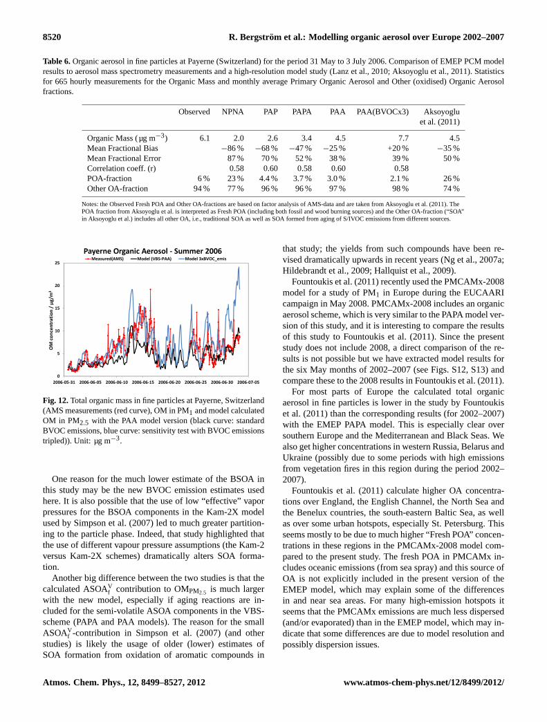
8520 R. Bergstrom et al.: Modelling organic aerosol over Europe 2002–2007
Table 6.Organic aerosol in fine particles at Payerne (Switzerland) for the period 31 May to 3 July 2006. Comparison of EMEP PCM modelresults to aerosol mass spectrometry measurements and a high-resolution model study (Lanz et al., 2010; Aksoyoglu et al., 2011). Statisticsfor 665 hourly measurements for the Organic Mass and monthly average Primary Organic Aerosol and Other (oxidised) Organic Aerosolfractions.
Observed NPNA PAP PAPA PAA PAA(BVOCx3) Aksoyogluet al. (2011)
Organic Mass (µg m−3) 6.1 2.0 2.6 3.4 4.5 7.7 4.5Mean Fractional Bias −86 % −68 % −47 % −25 % +20 % −35 %Mean Fractional Error 87 % 70 % 52 % 38 % 39 % 50 %Correlation coeff. (r) 0.58 0.60 0.58 0.60 0.58POA-fraction 6 % 23 % 4.4 % 3.7 % 3.0 % 2.1 % 26 %Other OA-fraction 94 % 77 % 96 % 96 % 97 % 98 % 74 %
Notes: the Observed Fresh POA and Other OA-fractions are based on factor analysis of AMS-data and are taken fromAksoyoglu et al.(2011). ThePOA fraction fromAksoyoglu et al.is interpreted as Fresh POA (including both fossil and wood burning sources) and the Other OA-fraction (“SOA”in Aksoyoglu et al.) includes all other OA, i.e., traditional SOA as well as SOA formed from aging of S/IVOC emissions from different sources.
0
5
10
15
20
25
2006-05-31 2006-06-05 2006-06-10 2006-06-15 2006-06-20 2006-06-25 2006-06-30 2006-07-05
OM
co
nce
ntr
ati
on
/ µ
g/m
3
Payerne Organic Aerosol - Summer 2006Measured(AMS) Model (VBS-PAA) Model 3xBVOC_emis
Fig. 12: Total organic mass in fine particles at Payerne, Switzerland (AMS measurements (red
curve), PM1 and model calculated OM in PM2.5 with the PAA model version (black curve: standard
BVOC emissions, blue curve: sensitivity test with BVOC emissions tripled)). Unit: µg m−3.
Table 6: Organic aerosol in fine particles at Payerne (Switzerland) for the period 31 May to 3 July
2006. Comparison of EMEP PCM model results to aerosol mass spectrometry measurements and
a high-resolution model study (Lanz et al., 2010; Aksoyogluet al., 2011). Statistics for 665 hourly
measurements for the Organic Mass and monthly average Primary Organic Aerosol and Other (oxi-
dised) Organic Aerosol fractions.
Observed NPNA PAP PAPA PAA PAA(BVOCx3) Aksoyoglu
et al., 2011
Organic Mass (µg m−3) 6.1 2.0 2.6 3.4 4.5 7.7 4.5
Mean Fractional Bias -86% -68% -47% -25% +20% -35%
Mean Fractional Error 87% 70% 52% 38% 39% 50%
Correlation coeff. (r) 0.58 0.60 0.58 0.60 0.58
POA-fraction 6% 23% 4.4% 3.7% 3.0% 2.1% 26%
Other OA-fraction 94% 77% 96% 96% 97% 98% 74%
Notes: The Observed Fresh POA and Other OA-fractions are based on factor analysis of AMS-data and are taken from Aksoyoglu et al. (2011).
The POA fraction from Aksoyoglu et al. is interpreted as Fresh POA (including bothfossil and wood burning sources) and the Other OA-
fraction (“SOA” in Aksoyoglu et al.) includes all other OA, i.e., traditional SOA as well as SOA formed from aging of S/IVOC emissions from
different sources.
37
Fig. 12.Total organic mass in fine particles at Payerne, Switzerland(AMS measurements (red curve), OM in PM1 and model calculatedOM in PM2.5 with the PAA model version (black curve: standardBVOC emissions, blue curve: sensitivity test with BVOC emissionstripled)). Unit: µg m−3.
One reason for the much lower estimate of the BSOA inthis study may be the new BVOC emission estimates usedhere. It is also possible that the use of low “effective” vaporpressures for the BSOA components in the Kam-2X modelused bySimpson et al.(2007) led to much greater partition-ing to the particle phase. Indeed, that study highlighted thatthe use of different vapour pressure assumptions (the Kam-2versus Kam-2X schemes) dramatically alters SOA forma-tion.
Another big difference between the two studies is that thecalculated ASOAVf contribution to OMPM2.5 is much largerwith the new model, especially if aging reactions are in-cluded for the semi-volatile ASOA components in the VBS-scheme (PAPA and PAA models). The reason for the smallASOAV
f -contribution in Simpson et al.(2007) (and otherstudies) is likely the usage of older (lower) estimates ofSOA formation from oxidation of aromatic compounds in
that study; the yields from such compounds have been re-vised dramatically upwards in recent years (Ng et al., 2007a;Hildebrandt et al., 2009; Hallquist et al., 2009).
Fountoukis et al.(2011) recently used the PMCAMx-2008model for a study of PM1 in Europe during the EUCAARIcampaign in May 2008. PMCAMx-2008 includes an organicaerosol scheme, which is very similar to the PAPA model ver-sion of this study, and it is interesting to compare the resultsof this study toFountoukis et al.(2011). Since the presentstudy does not include 2008, a direct comparison of the re-sults is not possible but we have extracted model results forthe six May months of 2002–2007 (see Figs. S12, S13) andcompare these to the 2008 results inFountoukis et al.(2011).
For most parts of Europe the calculated total organicaerosol in fine particles is lower in the study byFountoukiset al.(2011) than the corresponding results (for 2002–2007)with the EMEP PAPA model. This is especially clear oversouthern Europe and the Mediterranean and Black Seas. Wealso get higher concentrations in western Russia, Belarus andUkraine (possibly due to some periods with high emissionsfrom vegetation fires in this region during the period 2002–2007).
Fountoukis et al.(2011) calculate higher OA concentra-tions over England, the English Channel, the North Sea andthe Benelux countries, the south-eastern Baltic Sea, as wellas over some urban hotspots, especially St. Petersburg. Thisseems mostly to be due to much higher “Fresh POA” concen-trations in these regions in the PMCAMx-2008 model com-pared to the present study. The fresh POA in PMCAMx in-cludes oceanic emissions (from sea spray) and this source ofOA is not explicitly included in the present version of theEMEP model, which may explain some of the differencesin and near sea areas. For many high-emission hotspots itseems that the PMCAMx emissions are much less dispersed(and/or evaporated) than in the EMEP model, which may in-dicate that some differences are due to model resolution andpossibly dispersion issues.
Atmos. Chem. Phys., 12, 8499–8527, 2012 www.atmos-chem-phys.net/12/8499/2012/
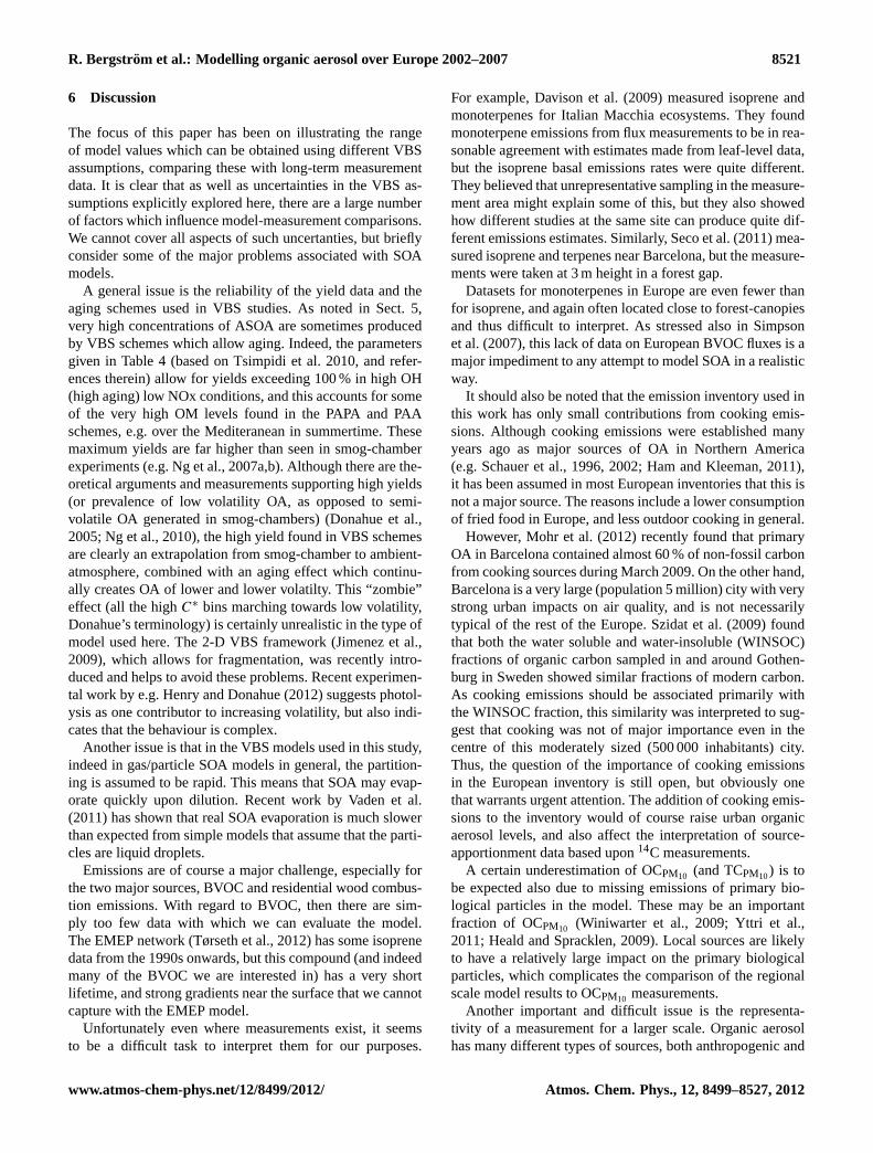
R. Bergstrom et al.: Modelling organic aerosol over Europe 2002–2007 8521
6 Discussion
The focus of this paper has been on illustrating the rangeof model values which can be obtained using different VBSassumptions, comparing these with long-term measurementdata. It is clear that as well as uncertainties in the VBS as-sumptions explicitly explored here, there are a large numberof factors which influence model-measurement comparisons.We cannot cover all aspects of such uncertanties, but brieflyconsider some of the major problems associated with SOAmodels.
A general issue is the reliability of the yield data and theaging schemes used in VBS studies. As noted in Sect.5,very high concentrations of ASOA are sometimes producedby VBS schemes which allow aging. Indeed, the parametersgiven in Table4 (based onTsimpidi et al.2010, and refer-ences therein) allow for yields exceeding 100 % in high OH(high aging) low NOx conditions, and this accounts for someof the very high OM levels found in the PAPA and PAAschemes, e.g. over the Mediteranean in summertime. Thesemaximum yields are far higher than seen in smog-chamberexperiments (e.g.Ng et al., 2007a,b). Although there are the-oretical arguments and measurements supporting high yields(or prevalence of low volatility OA, as opposed to semi-volatile OA generated in smog-chambers) (Donahue et al.,2005; Ng et al., 2010), the high yield found in VBS schemesare clearly an extrapolation from smog-chamber to ambient-atmosphere, combined with an aging effect which continu-ally creates OA of lower and lower volatilty. This “zombie”effect (all the highC∗ bins marching towards low volatility,Donahue’s terminology) is certainly unrealistic in the type ofmodel used here. The 2-D VBS framework (Jimenez et al.,2009), which allows for fragmentation, was recently intro-duced and helps to avoid these problems. Recent experimen-tal work by e.g.Henry and Donahue(2012) suggests photol-ysis as one contributor to increasing volatility, but also indi-cates that the behaviour is complex.
Another issue is that in the VBS models used in this study,indeed in gas/particle SOA models in general, the partition-ing is assumed to be rapid. This means that SOA may evap-orate quickly upon dilution. Recent work byVaden et al.(2011) has shown that real SOA evaporation is much slowerthan expected from simple models that assume that the parti-cles are liquid droplets.
Emissions are of course a major challenge, especially forthe two major sources, BVOC and residential wood combus-tion emissions. With regard to BVOC, then there are sim-ply too few data with which we can evaluate the model.The EMEP network (Tørseth et al., 2012) has some isoprenedata from the 1990s onwards, but this compound (and indeedmany of the BVOC we are interested in) has a very shortlifetime, and strong gradients near the surface that we cannotcapture with the EMEP model.
Unfortunately even where measurements exist, it seemsto be a difficult task to interpret them for our purposes.
For example,Davison et al.(2009) measured isoprene andmonoterpenes for Italian Macchia ecosystems. They foundmonoterpene emissions from flux measurements to be in rea-sonable agreement with estimates made from leaf-level data,but the isoprene basal emissions rates were quite different.They believed that unrepresentative sampling in the measure-ment area might explain some of this, but they also showedhow different studies at the same site can produce quite dif-ferent emissions estimates. Similarly,Seco et al.(2011) mea-sured isoprene and terpenes near Barcelona, but the measure-ments were taken at 3 m height in a forest gap.
Datasets for monoterpenes in Europe are even fewer thanfor isoprene, and again often located close to forest-canopiesand thus difficult to interpret. As stressed also inSimpsonet al.(2007), this lack of data on European BVOC fluxes is amajor impediment to any attempt to model SOA in a realisticway.
It should also be noted that the emission inventory used inthis work has only small contributions from cooking emis-sions. Although cooking emissions were established manyyears ago as major sources of OA in Northern America(e.g.Schauer et al., 1996, 2002; Ham and Kleeman, 2011),it has been assumed in most European inventories that this isnot a major source. The reasons include a lower consumptionof fried food in Europe, and less outdoor cooking in general.
However,Mohr et al.(2012) recently found that primaryOA in Barcelona contained almost 60 % of non-fossil carbonfrom cooking sources during March 2009. On the other hand,Barcelona is a very large (population 5 million) city with verystrong urban impacts on air quality, and is not necessarilytypical of the rest of the Europe.Szidat et al.(2009) foundthat both the water soluble and water-insoluble (WINSOC)fractions of organic carbon sampled in and around Gothen-burg in Sweden showed similar fractions of modern carbon.As cooking emissions should be associated primarily withthe WINSOC fraction, this similarity was interpreted to sug-gest that cooking was not of major importance even in thecentre of this moderately sized (500 000 inhabitants) city.Thus, the question of the importance of cooking emissionsin the European inventory is still open, but obviously onethat warrants urgent attention. The addition of cooking emis-sions to the inventory would of course raise urban organicaerosol levels, and also affect the interpretation of source-apportionment data based upon14C measurements.
A certain underestimation of OCPM10 (and TCPM10) is tobe expected also due to missing emissions of primary bio-logical particles in the model. These may be an importantfraction of OCPM10 (Winiwarter et al., 2009; Yttri et al.,2011; Heald and Spracklen, 2009). Local sources are likelyto have a relatively large impact on the primary biologicalparticles, which complicates the comparison of the regionalscale model results to OCPM10 measurements.
Another important and difficult issue is the representa-tivity of a measurement for a larger scale. Organic aerosolhas many different types of sources, both anthropogenic and
www.atmos-chem-phys.net/12/8499/2012/ Atmos. Chem. Phys., 12, 8499–8527, 2012
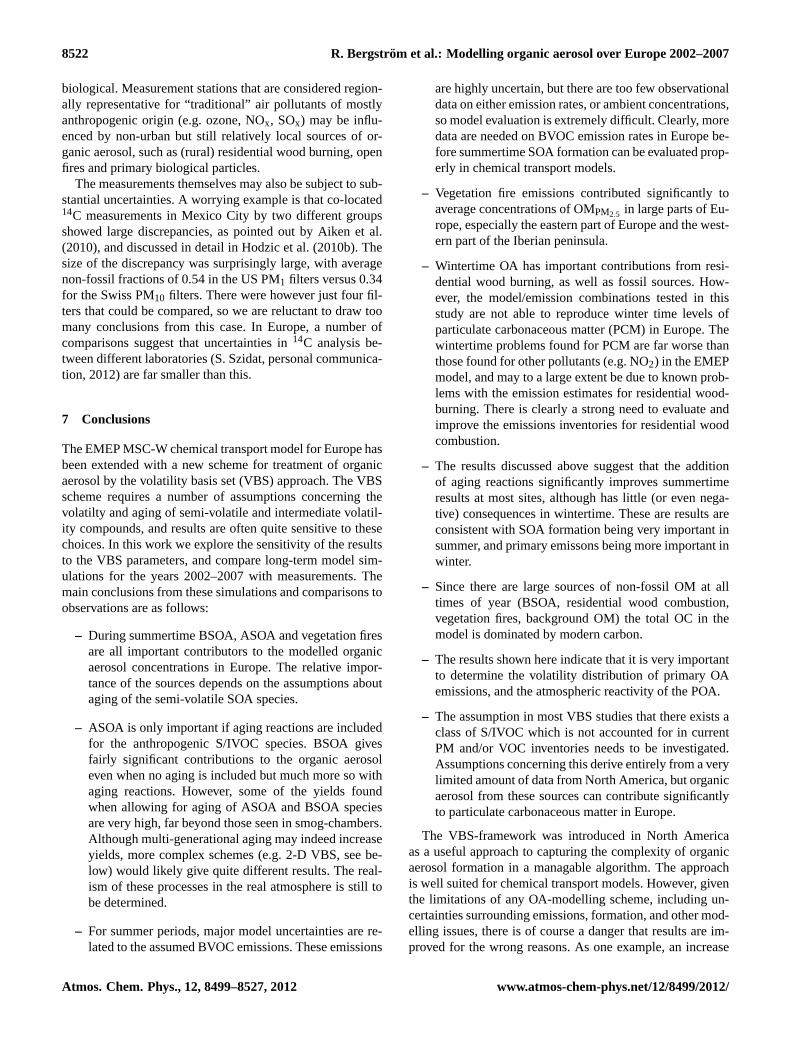
8522 R. Bergstrom et al.: Modelling organic aerosol over Europe 2002–2007
biological. Measurement stations that are considered region-ally representative for “traditional” air pollutants of mostlyanthropogenic origin (e.g. ozone, NOx, SOx) may be influ-enced by non-urban but still relatively local sources of or-ganic aerosol, such as (rural) residential wood burning, openfires and primary biological particles.
The measurements themselves may also be subject to sub-stantial uncertainties. A worrying example is that co-located14C measurements in Mexico City by two different groupsshowed large discrepancies, as pointed out byAiken et al.(2010), and discussed in detail inHodzic et al.(2010b). Thesize of the discrepancy was surprisingly large, with averagenon-fossil fractions of 0.54 in the US PM1 filters versus 0.34for the Swiss PM10 filters. There were however just four fil-ters that could be compared, so we are reluctant to draw toomany conclusions from this case. In Europe, a number ofcomparisons suggest that uncertainties in14C analysis be-tween different laboratories (S. Szidat, personal communica-tion, 2012) are far smaller than this.
7 Conclusions
The EMEP MSC-W chemical transport model for Europe hasbeen extended with a new scheme for treatment of organicaerosol by the volatility basis set (VBS) approach. The VBSscheme requires a number of assumptions concerning thevolatilty and aging of semi-volatile and intermediate volatil-ity compounds, and results are often quite sensitive to thesechoices. In this work we explore the sensitivity of the resultsto the VBS parameters, and compare long-term model sim-ulations for the years 2002–2007 with measurements. Themain conclusions from these simulations and comparisons toobservations are as follows:
– During summertime BSOA, ASOA and vegetation firesare all important contributors to the modelled organicaerosol concentrations in Europe. The relative impor-tance of the sources depends on the assumptions aboutaging of the semi-volatile SOA species.
– ASOA is only important if aging reactions are includedfor the anthropogenic S/IVOC species. BSOA givesfairly significant contributions to the organic aerosoleven when no aging is included but much more so withaging reactions. However, some of the yields foundwhen allowing for aging of ASOA and BSOA speciesare very high, far beyond those seen in smog-chambers.Although multi-generational aging may indeed increaseyields, more complex schemes (e.g. 2-D VBS, see be-low) would likely give quite different results. The real-ism of these processes in the real atmosphere is still tobe determined.
– For summer periods, major model uncertainties are re-lated to the assumed BVOC emissions. These emissions
are highly uncertain, but there are too few observationaldata on either emission rates, or ambient concentrations,so model evaluation is extremely difficult. Clearly, moredata are needed on BVOC emission rates in Europe be-fore summertime SOA formation can be evaluated prop-erly in chemical transport models.
– Vegetation fire emissions contributed significantly toaverage concentrations of OMPM2.5 in large parts of Eu-rope, especially the eastern part of Europe and the west-ern part of the Iberian peninsula.
– Wintertime OA has important contributions from resi-dential wood burning, as well as fossil sources. How-ever, the model/emission combinations tested in thisstudy are not able to reproduce winter time levels ofparticulate carbonaceous matter (PCM) in Europe. Thewintertime problems found for PCM are far worse thanthose found for other pollutants (e.g. NO2) in the EMEPmodel, and may to a large extent be due to known prob-lems with the emission estimates for residential wood-burning. There is clearly a strong need to evaluate andimprove the emissions inventories for residential woodcombustion.
– The results discussed above suggest that the additionof aging reactions significantly improves summertimeresults at most sites, although has little (or even nega-tive) consequences in wintertime. These are results areconsistent with SOA formation being very important insummer, and primary emissons being more important inwinter.
– Since there are large sources of non-fossil OM at alltimes of year (BSOA, residential wood combustion,vegetation fires, background OM) the total OC in themodel is dominated by modern carbon.
– The results shown here indicate that it is very importantto determine the volatility distribution of primary OAemissions, and the atmospheric reactivity of the POA.
– The assumption in most VBS studies that there exists aclass of S/IVOC which is not accounted for in currentPM and/or VOC inventories needs to be investigated.Assumptions concerning this derive entirely from a verylimited amount of data from North America, but organicaerosol from these sources can contribute significantlyto particulate carbonaceous matter in Europe.
The VBS-framework was introduced in North Americaas a useful approach to capturing the complexity of organicaerosol formation in a managable algorithm. The approachis well suited for chemical transport models. However, giventhe limitations of any OA-modelling scheme, including un-certainties surrounding emissions, formation, and other mod-elling issues, there is of course a danger that results are im-proved for the wrong reasons. As one example, an increase
Atmos. Chem. Phys., 12, 8499–8527, 2012 www.atmos-chem-phys.net/12/8499/2012/
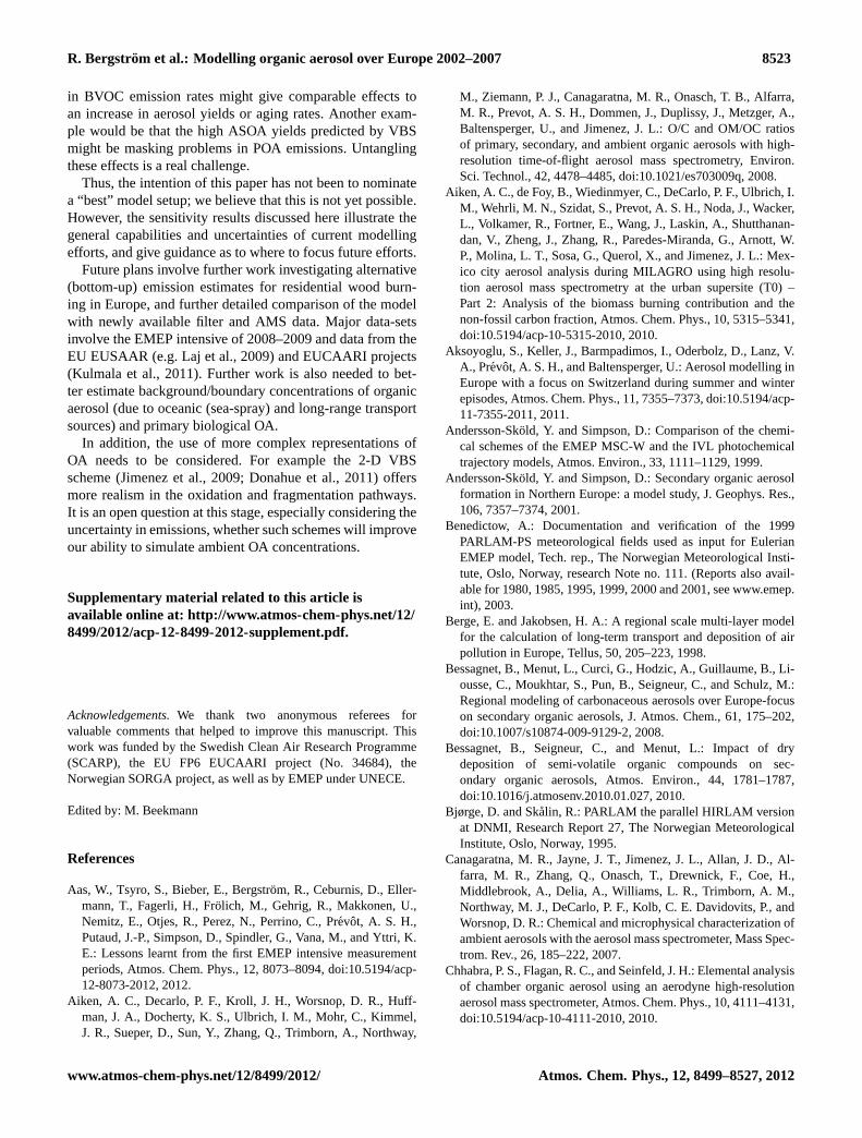
R. Bergstrom et al.: Modelling organic aerosol over Europe 2002–2007 8523
in BVOC emission rates might give comparable effects toan increase in aerosol yields or aging rates. Another exam-ple would be that the high ASOA yields predicted by VBSmight be masking problems in POA emissions. Untanglingthese effects is a real challenge.
Thus, the intention of this paper has not been to nominatea “best” model setup; we believe that this is not yet possible.However, the sensitivity results discussed here illustrate thegeneral capabilities and uncertainties of current modellingefforts, and give guidance as to where to focus future efforts.
Future plans involve further work investigating alternative(bottom-up) emission estimates for residential wood burn-ing in Europe, and further detailed comparison of the modelwith newly available filter and AMS data. Major data-setsinvolve the EMEP intensive of 2008–2009 and data from theEU EUSAAR (e.g.Laj et al., 2009) and EUCAARI projects(Kulmala et al., 2011). Further work is also needed to bet-ter estimate background/boundary concentrations of organicaerosol (due to oceanic (sea-spray) and long-range transportsources) and primary biological OA.
In addition, the use of more complex representations ofOA needs to be considered. For example the 2-D VBSscheme (Jimenez et al., 2009; Donahue et al., 2011) offersmore realism in the oxidation and fragmentation pathways.It is an open question at this stage, especially considering theuncertainty in emissions, whether such schemes will improveour ability to simulate ambient OA concentrations.
Supplementary material related to this article isavailable online at:http://www.atmos-chem-phys.net/12/8499/2012/acp-12-8499-2012-supplement.pdf.
Acknowledgements.We thank two anonymous referees forvaluable comments that helped to improve this manuscript. Thiswork was funded by the Swedish Clean Air Research Programme(SCARP), the EU FP6 EUCAARI project (No. 34684), theNorwegian SORGA project, as well as by EMEP under UNECE.
Edited by: M. Beekmann
References
Aas, W., Tsyro, S., Bieber, E., Bergstrom, R., Ceburnis, D., Eller-mann, T., Fagerli, H., Frolich, M., Gehrig, R., Makkonen, U.,Nemitz, E., Otjes, R., Perez, N., Perrino, C., Prevot, A. S. H.,Putaud, J.-P., Simpson, D., Spindler, G., Vana, M., and Yttri, K.E.: Lessons learnt from the first EMEP intensive measurementperiods, Atmos. Chem. Phys., 12, 8073–8094,doi:10.5194/acp-12-8073-2012, 2012.
Aiken, A. C., Decarlo, P. F., Kroll, J. H., Worsnop, D. R., Huff-man, J. A., Docherty, K. S., Ulbrich, I. M., Mohr, C., Kimmel,J. R., Sueper, D., Sun, Y., Zhang, Q., Trimborn, A., Northway,
M., Ziemann, P. J., Canagaratna, M. R., Onasch, T. B., Alfarra,M. R., Prevot, A. S. H., Dommen, J., Duplissy, J., Metzger, A.,Baltensperger, U., and Jimenez, J. L.: O/C and OM/OC ratiosof primary, secondary, and ambient organic aerosols with high-resolution time-of-flight aerosol mass spectrometry, Environ.Sci. Technol., 42, 4478–4485,doi:10.1021/es703009q, 2008.
Aiken, A. C., de Foy, B., Wiedinmyer, C., DeCarlo, P. F., Ulbrich, I.M., Wehrli, M. N., Szidat, S., Prevot, A. S. H., Noda, J., Wacker,L., Volkamer, R., Fortner, E., Wang, J., Laskin, A., Shutthanan-dan, V., Zheng, J., Zhang, R., Paredes-Miranda, G., Arnott, W.P., Molina, L. T., Sosa, G., Querol, X., and Jimenez, J. L.: Mex-ico city aerosol analysis during MILAGRO using high resolu-tion aerosol mass spectrometry at the urban supersite (T0) –Part 2: Analysis of the biomass burning contribution and thenon-fossil carbon fraction, Atmos. Chem. Phys., 10, 5315–5341,doi:10.5194/acp-10-5315-2010, 2010.
Aksoyoglu, S., Keller, J., Barmpadimos, I., Oderbolz, D., Lanz, V.A., Prevot, A. S. H., and Baltensperger, U.: Aerosol modelling inEurope with a focus on Switzerland during summer and winterepisodes, Atmos. Chem. Phys., 11, 7355–7373,doi:10.5194/acp-11-7355-2011, 2011.
Andersson-Skold, Y. and Simpson, D.: Comparison of the chemi-cal schemes of the EMEP MSC-W and the IVL photochemicaltrajectory models, Atmos. Environ., 33, 1111–1129, 1999.
Andersson-Skold, Y. and Simpson, D.: Secondary organic aerosolformation in Northern Europe: a model study, J. Geophys. Res.,106, 7357–7374, 2001.
Benedictow, A.: Documentation and verification of the 1999PARLAM-PS meteorological fields used as input for EulerianEMEP model, Tech. rep., The Norwegian Meteorological Insti-tute, Oslo, Norway, research Note no. 111. (Reports also avail-able for 1980, 1985, 1995, 1999, 2000 and 2001, seewww.emep.int), 2003.
Berge, E. and Jakobsen, H. A.: A regional scale multi-layer modelfor the calculation of long-term transport and deposition of airpollution in Europe, Tellus, 50, 205–223, 1998.
Bessagnet, B., Menut, L., Curci, G., Hodzic, A., Guillaume, B., Li-ousse, C., Moukhtar, S., Pun, B., Seigneur, C., and Schulz, M.:Regional modeling of carbonaceous aerosols over Europe-focuson secondary organic aerosols, J. Atmos. Chem., 61, 175–202,doi:10.1007/s10874-009-9129-2, 2008.
Bessagnet, B., Seigneur, C., and Menut, L.: Impact of drydeposition of semi-volatile organic compounds on sec-ondary organic aerosols, Atmos. Environ., 44, 1781–1787,doi:10.1016/j.atmosenv.2010.01.027, 2010.
Bjørge, D. and Skalin, R.: PARLAM the parallel HIRLAM versionat DNMI, Research Report 27, The Norwegian MeteorologicalInstitute, Oslo, Norway, 1995.
Canagaratna, M. R., Jayne, J. T., Jimenez, J. L., Allan, J. D., Al-farra, M. R., Zhang, Q., Onasch, T., Drewnick, F., Coe, H.,Middlebrook, A., Delia, A., Williams, L. R., Trimborn, A. M.,Northway, M. J., DeCarlo, P. F., Kolb, C. E. Davidovits, P., andWorsnop, D. R.: Chemical and microphysical characterization ofambient aerosols with the aerosol mass spectrometer, Mass Spec-trom. Rev., 26, 185–222, 2007.
Chhabra, P. S., Flagan, R. C., and Seinfeld, J. H.: Elemental analysisof chamber organic aerosol using an aerodyne high-resolutionaerosol mass spectrometer, Atmos. Chem. Phys., 10, 4111–4131,doi:10.5194/acp-10-4111-2010, 2010.
www.atmos-chem-phys.net/12/8499/2012/ Atmos. Chem. Phys., 12, 8499–8527, 2012
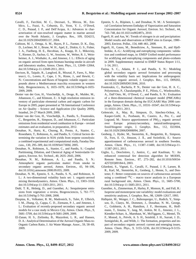
8524 R. Bergstrom et al.: Modelling organic aerosol over Europe 2002–2007
Cavalli, F., Facchini, M. C., Decesari, S., Mircea, M., Em-blico, L., Fuzzi, S., Ceburnis, D., Yoon, Y. J., O’Dowd,C. D., Putaud, J. P., and Dell’Acqua, A.: Advances in char-acterization of size-resolved organic matter in marine aerosolover the North Atlantic, J. Geophys. Res., 109, D24215,doi:10.1029/2004JD005137, 2004.
Cubison, M. J., Ortega, A. M., Hayes, P. L., Farmer, D. K., Day,D., Lechner, M. J., Brune, W. H., Apel, E., Diskin, G. S., Fisher,J. A., Fuelberg, H. E., Hecobian, A., Knapp, D. J., Mikoviny,T., Riemer, D., Sachse, G. W., Sessions, W., Weber, R. J., Wein-heimer, A. J., Wisthaler, A., and Jimenez, J. L.: Effects of agingon organic aerosol from open biomass burning smoke in aircraftand laboratory studies, Atmos. Chem. Phys., 11, 12049–12064,doi:10.5194/acp-11-12049-2011, 2011.
Davison, B., Taipale, R., Langford, B., Misztal, P., Fares, S., Mat-teucci, G., Loreto, F., Cape, J. N., Rinne, J., and Hewitt, C.N.: Concentrations and fluxes of biogenic volatile organic com-pounds above a Mediterranean macchia ecosystem in westernItaly, Biogeosciences, 6, 1655–1670,doi:10.5194/bg-6-1655-2009, 2009.
Denier van der Gon, H., Visschedijk, A., Droge, R., Mulder, M.,Johansson, C., and Klimont, Z.: A high resolution emission in-ventory of particulate elemental carbon and organic carbon forEurope in 2005, paper presented at 7th International Conferenceon Air Quality – Science and Application (Air Quality 2009),Istanbul, 24–27 March 2009, 2009.
Denier van der Gon, H., Visschedijk, A., Pandis, S., Fountoukis,C., Bergstrom, R., Simpson, D., and Johansson, C.: Particulateemissions from residential wood combustion in Europe – revisedestimates and an evaluation, in preparation, 2012.
Donahue, N., Hartz, K., Chuong, B., Presto, A., Stanier, C.,Rosenhørn, T., Robinson, A., and Pandis, S.: Critical factors de-termining the variation in SOA yields from terpene ozonolysis:a combined experimental and computational study, Faraday Dis-cuss., 130, 295–309,doi:10.1039/b417369d, 2005.
Donahue, N., Robinson, A., Stanier, C., and Pandis, S.: CoupledPartitioning, Dilution, and Chemical Aging of Semivolatile Or-ganics, Environ. Sci. Technol., 40, 2635–2643, 2006.
Donahue, N. M., Robinson, A. L., and Pandis, S. N.:Atmospheric organic particulate matter: From smoke tosecondary organic aerosol, Atmos. Environ., 43, 94–106,doi:10.1016/j.atmosenv.2008.09.055, 2009.
Donahue, N. M., Epstein, S. A., Pandis, S. N., and Robinson, A.L.: A two-dimensional volatility basis set: 1. organic-aerosolmixing thermodynamics, Atmos. Chem. Phys., 11, 3303–3318,doi:10.5194/acp-11-3303-2011, 2011.
Duhl, T. R., Helmig, D., and Guenther, A.: Sesquiterpene emis-sions from vegetation: a review, Biogeosciences, 5, 761–777,doi:10.5194/bg-5-761-2008, 2008.
Dzepina, K., Volkamer, R. M., Madronich, S., Tulet, P., Ulbrich,I. M., Zhang, Q., Cappa, C. D., Ziemann, P. J., and Jimenez, J.L.: Evaluation of recently-proposed secondary organic aerosolmodels for a case study in Mexico City, Atmos. Chem. Phys., 9,5681–5709,doi:10.5194/acp-9-5681-2009, 2009.
El-Zanan, H. S., Zielinska, B., Mazzoleni, L. R., and Hansen,D. A.: Analytical Determination of the Aerosol Organic Mass-to-Organic Carbon Ratio, J. Air Waste Manage. Assoc., 59, 58–69,2009.
Epstein, S. A., Riipinen, I., and Donahue, N. M.: A Semiempiri-cal Correlation between Enthalpy of Vaporization and SaturationConcentration for Organic Aerosol, Environ. Sci. Technol., 44,743–748,doi:10.1021/es902497z, 2010.
Fagerli, H. and Aas, W.: Trends of nitrogen in air and precipitation:Model results and observations at EMEP sites in Europe, 1980–2003, Environ. Pollut., 154, 448–461, 2008.
Fagerli, H., Gauss, M., Benedictow, A., Steensen, B., and Hjell-brekke, A.-G.: Acidifying and eutrophying components: valida-tion and combined maps, in: EMEP Unified model performancefor acidifying and eutrophying components and photo-oxidantsin 2009. Supplementary material to EMEP Status Report 1/11,1–54, 2011.
Farina, S. C., Adams, P. J., and Pandis, S. N.: Modelingglobal secondary organic aerosol formation and processingwith the volatility basis set: Implications for anthropogenicsecondary organic aerosol, J. Geophys. Res., 115, D09202,doi:10.1029/2009JD013046, 2010.
Fountoukis, C., Racherla, P. N., Denier van der Gon, H. A. C.,Polymeneas, P., Charalampidis, P. E., Pilinis, C., Wiedensohler,A., Dall’Osto, M., O’Dowd, C., and Pandis, S. N.: Evaluationof a three-dimensional chemical transport model (PMCAMx)in the European domain during the EUCAARI May 2008 cam-paign, Atmos. Chem. Phys., 11, 10331–10347,doi:10.5194/acp-11-10331-2011, 2011.
Gelencser, A., May, B., Simpson, D., Sanchez-Ochoa, A.,Kasper-Giebl, A., Puxbaum, H., Caseiro, A., Pio, C., andLegrand, M.: Source apportionment of PM2.5 organic aerosolover Europe: primary/secondary, natural/anthropogenic,fossil/biogenic origin, J. Geophys. Res., 112, D23S04,doi:10.1029/2006JD008094, 2007.
Genberg, J., Hyder, M., Stenstrom, K., Bergstrom, R., Simpson,D., Fors, E. O., Jonsson, J.A., and Swietlicki, E.: Sourceapportionment of carbonaceous aerosol in southern Sweden,Atmos. Chem. Phys., 11, 11387–11400,doi:10.5194/acp-11-11387-2011, 2011.
Giglio, L., Descloitres, J., Justice, C., and Kaufman, Y.: Anenhanced contextual fire detection algorithm for MODIS,Remote Sens. Environ., 87, 273–282,doi:10.1016/S0034-4257(03)00184-6, 2003.
Gilardoni, S., Vignati, E., Cavalli, F., Putaud, J. P., Larsen, B.R., Karl, M., Stenstrom, K., Genberg, J., Henne, S., and Den-tener, F.: Better constraints on sources of carbonaceous aerosolsusing a combined14C – macro tracer analysis in a Europeanrural background site, Atmos. Chem. Phys., 11, 5685–5700,doi:10.5194/acp-11-5685-2011, 2011.
Guenther, A., Zimmerman, P., Harley, P., Monson, R., and Fall, R.:Isoprene and monoterpene rate variability: model evaluations andsensitivity analyses, J. Geophys. Res., 98, 12609–12617, 1993.
Hallquist, M., Wenger, J. C., Baltensperger, U., Rudich, Y., Simp-son, D., Claeys, M., Dommen, J., Donahue, N. M., George,C., Goldstein, A. H., Hamilton, J. F., Herrmann, H., Hoff-mann, T., Iinuma, Y., Jang, M., Jenkin, M. E., Jimenez, J. L.,Kiendler-Scharr, A., Maenhaut, W., McFiggans, G., Mentel, Th.F., Monod, A., Prevot, A. S. H., Seinfeld, J. H., Surratt, J. D.,Szmigielski, R., and Wildt, J.: The formation, properties and im-pact of secondary organic aerosol: current and emerging issues,Atmos. Chem. Phys., 9, 5155–5236,doi:10.5194/acp-9-5155-2009, 2009.
Atmos. Chem. Phys., 12, 8499–8527, 2012 www.atmos-chem-phys.net/12/8499/2012/

R. Bergstrom et al.: Modelling organic aerosol over Europe 2002–2007 8525
Ham, W. A. and Kleeman, M. J.: Size-resolved source appor-tionment of carbonaceous particulate matter in urban and ru-ral sites in central California, Atmos. Environ., 45, 3988–3995,doi:10.1016/j.atmosenv.2011.04.063, 2011.
Heald, C. L. and Spracklen, D. V.: Atmospheric budget of primarybiological aerosol particles from fungal spores, Geophys. Res.Lett., 36, L09806,doi:10.1029/2009GL037493, 2009.
Heintzenberg, J.: Fine particles in the global troposphere – a review,Tellus, 41B, 149–160, 1989.
Henry, K. and Donahue, N.: Photochenical aging ofα-pinene sec-ondary organic aerosol: effects of OH radical sources and pho-tolysis, J. Phys. Chem., 116, 5932–5940, 2012.
Hildebrandt, L., Donahue, N. M., and Pandis, S. N.: High forma-tion of secondary organic aerosol from the photo-oxidation oftoluene, Atmos. Chem. Phys., 9, 2973–2986,doi:10.5194/acp-9-2973-2009, 2009.
Hodzic, A., Jimenez, J. L., Madronich, S., Canagaratna, M. R., De-Carlo, P. F., Kleinman, L., and Fast, J.: Modeling organic aerosolsin a megacity: potential contribution of semi-volatile and inter-mediate volatility primary organic compounds to secondary or-ganic aerosol formation, Atmos. Chem. Phys., 10, 5491–5514,doi:10.5194/acp-10-5491-2010, 2010a.
Hodzic, A., Jimenez, J. L., Prevot, A. S. H., Szidat, S., Fast, J.D., and Madronich, S.: Can 3-D models explain the observedfractions of fossil and non-fossil carbon in and near MexicoCity?, Atmos. Chem. Phys., 10, 10997–11016,doi:10.5194/acp-10-10997-2010, 2010b.
Jimenez, J. L., Canagaratna, M. R., Donahue, N. M., Prevot, A.S. H., Zhang, Q., Kroll, J. H., DeCarlo, P. F., Allan, J. D., Coe,H., Ng, N. L., Aiken, A. C., Docherty, K. S., Ulbrich, I. M.,Grieshop, A. P., Robinson, A. L., Duplissy, J., Smith, J. D.,Wilson, K. R., Lanz, V. A., Hueglin, C., Sun, Y. L., Tian, J.,Laaksonen, A., Raatikainen, T., Rautiainen, J., Vaattovaara, P.,Ehn, M., Kulmala, M., Tomlinson, J. M., Collins, D. R., Cu-bison, M. J., Dunlea, E. J., Huffman, J. A., Onasch, T. B., Al-farra, M. R., Williams, P. I., Bower, K., Kondo, Y., Schneider, J.,Drewnick, F., Borrmann, S., Weimer, S., Demerjian, K., Salcedo,D., Cottrell, L., Griffin, R., Takami, A., Miyoshi, T., Hatakeyama,S., Shimono, A., Sun, J. Y., Zhang, Y. M., Dzepina, K., Kim-mel, J. R., Sueper, D., Jayne, J. T., Herndon, S. C., Trimborn,A. M., Williams, L. R., Wood, E. C., Middlebrook, A. M., Kolb,C. E., Baltensperger, U., and Worsnop, D. R.: Evolution of Or-ganic Aerosols in the Atmosphere, Science, 326, 1525–1529,doi:10.1126/science.1180353, 2009.
Jonson, J. E., Simpson, D., Fagerli, H., and Solberg, S.: Can we ex-plain the trends in European ozone levels?, Atmos. Chem. Phys.,6, 51–66,doi:10.5194/acp-6-51-2006, 2006.
Kanakidou, M., Seinfeld, J. H., Pandis, S. N., Barnes, I., Dentener,F. J., Facchini, M. C., Van Dingenen, R., Ervens, B., Nenes, A.,Nielsen, C. J., Swietlicki, E., Putaud, J. P., Balkanski, Y., Fuzzi,S., Horth, J., Moortgat, G. K., Winterhalter, R., Myhre, C. E.L., Tsigaridis, K., Vignati, E., Stephanou, E. G., and Wilson,J.: Organic aerosol and global climate modelling: a review, At-mos. Chem. Phys., 5, 1053–1123,doi:10.5194/acp-5-1053-2005,2005.
Karl, M., Guenther, A., Koble, R., Leip, A., and Seufert, G.: A newEuropean plant-specific emission inventory of biogenic volatileorganic compounds for use in atmospheric transport models, Bio-geosciences, 6, 1059–1087,doi:10.5194/bg-6-1059-2009, 2009.
Kesik, M., Ambus, P., Baritz, R., Bruggemann, N., Butterbach-Bahl, K., Damm, M., Duyzer, J., Horvath, L., Kiese, R., Kitzler,B., Leip, A., Li, C., Pihlatie, M., Pilegaard, K., Seufert, S., Simp-son, D., Skiba, U., Smiatek, G., Vesala, T., and Zechmeister-Boltenstern, S.: Inventories of N2O and NO emissions from Eu-ropean forest soils, Biogeosciences, 2, 353–375,doi:10.5194/bg-2-353-2005, 2005.
Kleefeld, S., Hofferb, A., Krivacsy, Z., and Jennings, S.: Importanceof organic and black carbon in atmospheric aerosols at MaceHead, on the West Coast of Ireland (53◦ 19′ N, 9◦ 54′ W), At-mos. Environ., 36, 4479–4490, 2002.
Koble, R. and Seufert, G.: Novel Maps for Forest TreeSpecies in Europe., in: A Changing Atmosphere, 8th Euro-pean Symposium on the Physico-Chemical Behaviour of Atmo-spheric Pollutants, Torino, Italy, 17–20 September 2001., avail-able at: http://ies.jrc.ec.europa.eu/Units/cc/events/torino2001/torinocd/Documents/Terrestrial/TP35.htm(last access: February2012), 2001.
Kulmala, M., Asmi, A., Lappalainen, H. K., Baltensperger, U.,Brenguier, J.-L., Facchini, M. C., Hansson, H.-C., Hov, Ø.,O’Dowd, C. D., Poschl, U., Wiedensohler, A., Boers, R.,Boucher, O., de Leeuw, G., Denier van der Gon, H. A. C., Fe-ichter, J., Krejci, R., Laj, P., Lihavainen, H., Lohmann, U., Mc-Figgans, G., Mentel, T., Pilinis, C., Riipinen, I., Schulz, M.,Stohl, A., Swietlicki, E., Vignati, E., Alves, C., Amann, M.,Ammann, M., Arabas, S., Artaxo, P., Baars, H., Beddows, D.C. S., Bergstrom, R., Beukes, J. P., Bilde, M., Burkhart, J. F.,Canonaco, F., Clegg, S. L., Coe, H., Crumeyrolle, S., D’Anna,B., Decesari, S., Gilardoni, S., Fischer, M., Fjaeraa, A. M., Foun-toukis, C., George, C., Gomes, L., Halloran, P., Hamburger, T.,Harrison, R. M., Herrmann, H., Hoffmann, T., Hoose, C., Hu,M., Hyvarinen, A., Horrak, U., Iinuma, Y., Iversen, T., Josipovic,M., Kanakidou, M., Kiendler-Scharr, A., Kirkevag, A., Kiss, G.,Klimont, Z., Kolmonen, P., Komppula, M., Kristjansson, J.-E.,Laakso, L., Laaksonen, A., Labonnote, L., Lanz, V. A., Lehtinen,K. E. J., Rizzo, L. V., Makkonen, R., Manninen, H. E., McMeek-ing, G., Merikanto, J., Minikin, A., Mirme, S., Morgan, W. T.,Nemitz, E., O’Donnell, D., Panwar, T. S., Pawlowska, H., Pet-zold, A., Pienaar, J. J., Pio, C., Plass-Duelmer, C., Prevot, A.S. H., Pryor, S., Reddington, C. L., Roberts, G., Rosenfeld, D.,Schwarz, J., Seland, Ø., Sellegri, K., Shen, X. J., Shiraiwa, M.,Siebert, H., Sierau, B., Simpson, D., Sun, J. Y., Topping, D.,Tunved, P., Vaattovaara, P., Vakkari, V., Veefkind, J. P., Viss-chedijk, A., Vuollekoski, H., Vuolo, R., Wehner, B., Wildt, J.,Woodward, S., Worsnop, D. R., van Zadelhoff, G.-J., Zardini,A. A., Zhang, K., van Zyl, P. G., Kerminen, V.-M., Carslaw, S.,K., and Pandis, S. N.: General overview: European Integratedproject on Aerosol Cloud Climate and Air Quality interactions(EUCAARI) – integrating aerosol research from nano to globalscales, Atmos. Chem. Phys., 11, 13061–13143,doi:10.5194/acp-11-13061-2011, 2011.
Kupiainen, K. and Klimont, Z.: Primary emissions of submicronand carbonaceous particles and the potential for their control.,IIASA IR-04-079, International Institute for Applied SystemsAnalysis (IIASA), 2004.
Kupiainen, K. and Klimont, Z.: Primary emissions of fine car-bonaceous particles in Europe, Atmos. Environ., 41, 2156–2170,doi:10.1016/j.atmosenv.2006.10.066, 2007.
www.atmos-chem-phys.net/12/8499/2012/ Atmos. Chem. Phys., 12, 8499–8527, 2012
8526 R. Bergstrom et al.: Modelling organic aerosol over Europe 2002–2007
Laj, P., Klausen, J., Bilde, M., Plaß-Duelmer, C., Pappalardo,G., Clerbaux, C., Baltensperger, U., Hjorth, J., Simpson, D.,Reimann, S., Coheur, P.-F., Richter, A., Maziere, M. D., Rudich,Y., McFiggans, G., Torseth, K., Wiedensohler, A., Morin, S.,Schulz, M., Allan, J., Attie, J.-L., Barnes, I., Birmilli, W., Cam-mas, P., Dommen, J., Dorn, H.-P., Fowler, D., Fuzzi, J.-S., Gla-sius, M., Granier, C., Hermann, M., Isaksen, I., Kinne, S., Ko-ren, I., Madonna, F., Maione, M., Massling, A., Moehler, O.,Mona, L., Monks, P., Muller, D., Muller, T., Orphal, J., Peuch,V.-H., Stratmann, F., Tanre, D., Tyndall, G., Riziq, A., Roozen-dael, M. V., Villani, P., Wehner, B., Wex, H., and Zardini, A.:Measuring Atmospheric Composition Change, Atmos. Environ.,43, 5351–5414,doi:10.1016/j.atmosenv.2009.08.020, 2009.
Lane, T. E., Donahue, N. M., and Pandis, S. N.: Effect of NOxon secondary organic aerosol concentrations, Environ. Sci. Tech-nol., 42, 6022–6027,doi:10.1021/es703225a, 2008a.
Lane, T. E., Donahue, N. M., and Pandis, S. N.: Simulating sec-ondary organic aerosol formation using the volatility basis-setapproach in a chemical transport model, Atmos. Environ., 42,7439–7451,doi:10.1016/j.atmosenv.2008.06.026, 2008b.
Lanz, V. A., Prevot, A. S. H., Alfarra, M. R., Weimer, S., Mohr,C., DeCarlo, P. F., Gianini, M. F. D., Hueglin, C., Schneider, J.,Favez, O., D’Anna, B., George, C., and Baltensperger, U.: Char-acterization of aerosol chemical composition with aerosol massspectrometry in Central Europe: an overview, Atmos. Chem.Phys., 10, 10453–10471,doi:10.5194/acp-10-10453-2010, 2010.
Legrand, M. and Puxbaum, H.: Summary of the CARBOSOLproject: Present and retrospective state of organic versus in-organic aerosol over Europe, J. Geophys. Res., 112, D23S01,doi:10.1029/2006JD008271, 2007.
Li, G., Bei, N., Tie, X., and Molina, L. T.: Aerosol ef-fects on the photochemistry in Mexico City during MCMA-2006/MILAGRO campaign, Atmos. Chem. Phys., 11, 5169–5182,doi:10.5194/acp-11-5169-2011, 2011.
McDonald, J. D., Eide, I., Seagrave, J., Zielinska, B., Whitney, K.,Lawson, D. R., and Mauderly, J. L.: Relationship between Com-position and Toxicity of Motor Vehicle Emission Samples, Env-iron. Health Persp., 112, 1527–1538, 2004.
McKay, M. D., Beckman, R. J., and Conover, W. J.: A Comparisonof Three Methods for Selecting Values of Input Variables in theAnalysis of Output from a Computer Code, Technometrics, 21,239–245,http://www.jstor.org/stable/1268522, 1979.
Mohr, C., DeCarlo, P. F., Heringa, M. F., Chirico, R., Slowik, J.G., Richter, R., Reche, C., Alastuey, A., Querol, X., Seco, R.,Penuelas, J., Jimenez, J. L., Crippa, M., Zimmermann, R., Bal-tensperger, U., and Prevot, A. S. H.: Identification and quan-tification of organic aerosol from cooking and other sources inBarcelona using aerosol mass spectrometer data, Atmos. Chem.Phys., 12, 1649–1665,doi:10.5194/acp-12-1649-2012, 2012.
Murphy, B. N. and Pandis, S. N.: Simulating the Formation ofSemivolatile Primary and Secondary Organic Aerosol in a Re-gional Chemical Transport Model, Environ. Sci. Technol., 43,4722–4728,doi:10.1021/es803168a, 2009.
Ng, N. L., Kroll, J. H., Chan, A. W. H., Chhabra, P. S., Flagan,R. C., and Seinfeld, J. H.: Secondary organic aerosol formationfrom m-xylene, toluene, and benzene, Atmos. Chem. Phys., 7,3909–3922,doi:10.5194/acp-7-3909-2007, 2007a.
Ng, N. L., Chhabra, P. S., Chan, A. W. H., Surratt, J. D., Kroll, J.H., Kwan, A. J., McCabe, D. C., Wennberg, P. O., Sorooshian,
A., Murphy, S. M., Dalleska, N. F., Flagan, R. C., and Seinfeld,J. H.: Effect of NOx level on secondary organic aerosol (SOA)formation from the photooxidation of terpenes, Atmos. Chem.Phys., 7, 5159–5174,doi:10.5194/acp-7-5159-2007, 2007b.
Ng, N. L., Canagaratna, M. R., Zhang, Q., Jimenez, J. L., Tian,J., Ulbrich, I. M., Kroll, J. H., Docherty, K. S., Chhabra, P.S., Bahreini, R., Murphy, S. M., Seinfeld, J. H., Hildebrandt,L., Donahue, N. M., DeCarlo, P. F., Lanz, V. A., Prevot, A. S.H., Dinar, E., Rudich, Y., and Worsnop, D. R.: Organic aerosolcomponents observed in Northern Hemispheric datasets fromAerosol Mass Spectrometry, Atmos. Chem. Phys., 10, 4625–4641,doi:10.5194/acp-10-4625-2010, 2010.
Novakov, T. and Penner, J.: Large contribution of organic aerosolsto cloud condensation nuclei concentrations, Nature, 365, 823–826, 1993.
Pathak, R. K., Presto, A. A., Lane, T. E., Stanier, C. O., Donahue, N.M., and Pandis, S. N.: Ozonolysis ofα-pinene: parameterizationof secondary organic aerosol mass fraction, Atmos. Chem. Phys.,7, 3811–3821,doi:10.5194/acp-7-3811-2007, 2007.
Pio, C. A., Legrand, M., Oliveira, T., Afonso, J., Santos, C., Ca-seiro, A., Fialho, P., Barata, F., Puxbaum, H., Sanchez-Ochoa, A.,Kasper-Giebl, A., Gelencser, A., Preunkert, S., and Schock, M.:Climatology of aerosol composition (organic versus inorganic) atnonurban sites on a west-east transect across Europe, J. Geophys.Res., 112, D23S02,doi:10.1029/2006JD008038, 2007.
Putaud, J.-P., Raes, F., Van Dingenen, R., Bruggemann, E., Fac-chini, M. C., Decesari, S., Fuzzi, S., Gehrig, R., Huglin, C.,Laj, P., Lorbeer, G., Maenhaut, W., Mihalopoulos, N., Muller,K., Querol, X., Rodriguez, S., Schneider, J., Spindler, G., Brink,H. t., Torseth, K., and Wiedensohler, A.: A European aerosolphenomenology-2: chemical characteristics of particulate matterat kerbside, urban, rural and background sites in Europe, Atmos.Environ., 38, 2579–2595, 2004.
Robinson, A. L., Donahue, N. M., Shrivastava, M. K., Weitkamp,E. A., Sage, A. M., Grieshop, A. P., Lane, T. E., Pierce, J. R.,and Pandis, S. N.: Rethinking Organic Aerosols: SemivolatileEmissions and Photochemical Aging, Science, 315, 1259–1262,doi:10.1126/science.1133061, 2007.
Seco, R., Penuelas, J., Filella, I., Llusia, J., Molowny-Horas, R.,Schallhart, S., Metzger, A., Muller, M., and Hansel, A.: Contrast-ing winter and summer VOC mixing ratios at a forest site in theWestern Mediterranean Basin: the effect of local biogenic emis-sions, Atmos. Chem. Phys., 11, 13161–13179,doi:10.5194/acp-11-13161-2011, 2011.
Schauer, J., Kleeman, M., Cass, G., and Simoneit, B.: Measurementof Emissions from Air Pollution Sources. 4. C1-C27 OrganicCompounds from Cooking with Seed Oils, Environ. Sci. Tech-nol., 36, 567–575, 2002.
Schauer, J. J., Rogge, W. F., Hildemann, L. M., Mazurek, M. A.,Cass, G. R., and Simoneit, B. R. T.: Source apportionment ofairborne particulate matter using organic compounds as tracers,Atmos. Environ., 30, 3837–3855, 1996.
Shrivastava, M., Fast, J., Easter, R., Gustafson Jr., W. I., Zaveri, R.A., Jimenez, J. L., Saide, P., and Hodzic, A.: Modeling organicaerosols in a megacity: comparison of simple and complex rep-resentations of the volatility basis set approach, Atmos. Chem.Phys., 11, 6639–6662,doi:10.5194/acp-11-6639-2011, 2011.
Shrivastava, M. K., Lane, T. E., Donahue, N. M., Pandis, S. N.,and Robinson, A. L.: Effects of gas particle partitioning
Atmos. Chem. Phys., 12, 8499–8527, 2012 www.atmos-chem-phys.net/12/8499/2012/
R. Bergstrom et al.: Modelling organic aerosol over Europe 2002–2007 8527
and aging of primary emissions on urban and regional or-ganic aerosol concentrations, J. Geophys. Res., 113, D18301doi:10.1029/2007JD009735, 2008.
Simon, H., Bhave, P. V., Swall, J. L., Frank, N. H., and Malm, W.C.: Determining the spatial and seasonal variability in OM/OCratios across the US using multiple regression, Atmos. Chem.Phys., 11, 2933–2949,doi:10.5194/acp-11-2933-2011, 2011.
Simpson, D., Winiwarter, W., Borjesson, G., Cinderby, S., Ferreiro,A., Guenther, A., Hewitt, C. N., Janson, R., Khalil, M. A. K.,Owen, S., Pierce, T. E., Puxbaum, H., Shearer, M., Skiba, U.,Steinbrecher, R., Tarrason, L., andOquist, M. G.: Inventoryingemissions from Nature in Europe, J. Geophys. Res., 104, 8113–8152, 1999.
Simpson, D., Fagerli, H., Jonson, J., Tsyro, S., Wind, P., and Tuovi-nen, J.-P.: The EMEP Unified Eulerian Model. Model Descrip-tion, EMEP MSC-W Report 1/2003, The Norwegian Meteoro-logical Institute, Oslo, Norway, 2003.
Simpson, D., Butterbach-Bahl, K., Fagerli, H., Kesik, M., Skiba,U., and Tang, S.: Deposition and Emissions of Reactive Nitrogenover European Forests: A Modelling Study, Atmos. Environ., 40,5712–5726,doi:10.1016/j.atmosenv.2006.04.063, 2006a.
Simpson, D., Fagerli, H., Hellsten, S., Knulst, J. C., and Westling,O.: Comparison of modelled and monitored deposition fluxesof sulphur and nitrogen to ICP-forest sites in Europe, Biogeo-sciences, 3, 337–355,doi:10.5194/bg-3-337-2006, 2006b.
Simpson, D., Yttri, K., Klimont, Z., Kupiainen, K., Caseiro, A.,Gelencser, A., Pio, C., and Legrand, M.: Modeling Carbona-ceous Aerosol over Europe. Analysis of the CARBOSOL andEMEP EC/OC campaigns, J. Geophys. Res., 112, D23S14,doi:10.1029/2006JD008158, 2007.
Simpson, D., Yttri, K., Bergstrom, R., and Denier van der Gon, H.:Modelling SOA in EMEP: Experiments with the VBS Approach,in: Transboundary Particulate Matter in Europe, Status Report4/2004, Tørseth, K. (ed.), EMEP CCC Report 4/2009, Norwe-gian Institute for Air Research, Kjeller, Norway, 2009.
Simpson, D., Benedictow, A., Berge, H., Bergstrom, R., Emberson,L. D., Fagerli, H., Flechard, C. R., Hayman, G. D., Gauss, M.,Jonson, J. E., Jenkin, M. E., Nyıri, A., Richter, C., Semeena, V.S., Tsyro, S., Tuovinen, J.-P., Valdebenito,A., and Wind, P.: TheEMEP MSC-W chemical transport model – technical descrip-tion, Atmos. Chem. Phys., 12, 7825–7865,doi:10.5194/acp-12-7825-2012, 2012.
Szidat, S., Ruff, M., Perron, N., Wacker, L., Synal, H.-A., Hallquist,M., Shannigrahi, A. S., Yttri, K. E., Dye, C., and Simpson, D.:Fossil and non-fossil sources of organic carbon (OC) and ele-mental carbon (EC) in Goteborg, Sweden, Atmos. Chem. Phys.,9, 1521–1535,doi:10.5194/acp-9-1521-2009, 2009.
Tarrason, L., Fagerli, H., Gauss, M., Nyıri, A., Simpson, D., Tsyro,S., and Aas, W.: S, N and O3 in EECCA countries, in: Trans-boundary Acidification, Eutrophication and Ground Level Ozonein Europe in 2006. EMEP Status Report 1/2008, pp. 67–86, TheNorwegian Meteorological Institute, Oslo, Norway, 2008.
Tørseth, K., Aas, W., Breivik, K., Fjæraa, A. M., Fiebig, M.,Hjellbrekke, A. G., Lund Myhre, C., Solberg, S., and Yttri,K. E.: Introduction to the European Monitoring and Evalua-tion Programme (EMEP) and observed atmospheric compositionchange during 1972–2009, Atmos. Chem. Phys., 12, 5447–5481,doi:10.5194/acp-12-5447-2012, 2012.
Tsimpidi, A. P., Karydis, V. A., Zavala, M., Lei, W., Molina, L.,Ulbrich, I. M., Jimenez, J. L., and Pandis, S. N.: Evaluation of thevolatility basis-set approach for the simulation of organic aerosolformation in the Mexico City metropolitan area, Atmos. Chem.Phys., 10, 525–546,doi:10.5194/acp-10-525-2010, 2010.
Tsyro, S., Simpson, D., Tarrason, L., Kupiainen, K., Klimont, Z.,Yttri, K., and Pio, C.: Modelling of black carbon over Europe, J.Geophys. Res., 112, D23S19,doi:10.1029/2006JD008164, 2007.
Turpin, B. J. and Lim, H. J.: Species contributions to PM2.5 massconcentrations: Revisiting common assumptions for estimatingorganic mass, Aerosol Sci. Technol., 35, 602–610, 2001.
UN-ECE: International Co-operative Programme on Assessmentand Monitoring of Air Pollution Effects on Forests. Manual onmethods and criteria for harmonized sampling, assessment, mon-itoring and analysis of the effects of air pollution on forests,updated version available at:(http://icp-forests.net)(last access:February 2012), 1998.
Vaden, T. D., Imre, D., Beranek, J., Shrivastava, M., and Zelenyuk,A.: Evaporation kinetics and phase of laboratory and ambientsecondary organic aerosol, P. Natl. Acad. Sci. USA, 108, 2190–2195, 2011.
van der Werf, G. R., Randerson, J. T., Giglio, L., Collatz, G. J.,Kasibhatla, P. S., and Arellano Jr., A. F.: Interannual variabil-ity in global biomass burning emissions from 1997 to 2004, At-mos. Chem. Phys., 6, 3423–3441,doi:10.5194/acp-6-3423-2006,2006.
Visschedijk, A. J. H., Denier van der Gon, H. A. C., Droge, R.,and Van der Brugh, H.: A European high resolution and size-differentiated emission inventory for elemental and organic car-bon for the year 2005, TNO TNO-034-UT-2009-00688PT-ML,TNO, Utrecht, The Netherlands, 2009.
Watson, J., Chow, J., and Chen, L.-W.: Summary of organic andelemental carbon/black carbon analysis methods and intercom-parisons, Aerosol Air Qual. Res., 5, 65–102, 2005.
Winiwarter, W., Bauer, H., Caseiro, A., and Puxbaum, H.:Quantifying emissions of primary biological aerosol par-ticle mass in Europe, Atmos. Environ., 43, 1403–1409,doi:10.1016/j.atmosenv.2008.01.037, 2009.
Yttri, K. E., Aas, W., Bjerke, A., Cape, J. N., Cavalli, F., Ceburnis,D., Dye, C., Emblico, L., Facchini, M. C., Forster, C., Hanssen,J. E., Hansson, H. C., Jennings, S. G., Maenhaut, W., Putaud,J. P., and Tørseth, K.: Elemental and organic carbon in PM10: aone year measurement campaign within the European Monitor-ing and Evaluation Programme EMEP, Atmos. Chem. Phys., 7,5711–5725,doi:10.5194/acp-7-5711-2007, 2007.
Yttri, K., Aas, W., Tørseth, K., Stebel, K., Nyıri, A., Tsyro, S., Mer-ckova, K., Wankmuller, R., Winiwarter, W., Bauer, H., Caseiro,A., Puxbaum, H., Holzer-Popp, T., and Schroedter-Homscheidt,M.: Transboundary particulate matter in Europe – Status report2008, EMEP Status Report 4/2008, NILU, available at:http://www.emep.int(last access: February 2012), 2008.
Yttri, K. E., Simpson, D., Stenstrom, K., Puxbaum, H., andSvendby, T.: Source apportionment of the carbonaceous aerosolin Norway – quantitative estimates based on14C, thermal-opticaland organic tracer analysis, Atmos. Chem. Phys., 11, 9375–9394,doi:10.5194/acp-11-9375-2011, 2011.
www.atmos-chem-phys.net/12/8499/2012/ Atmos. Chem. Phys., 12, 8499–8527, 2012