Modelling of hemodynamic timeseries and 2nd-level … · Modelling of hemodynamic timeseries and 2nd-level summary statistics ... SPM(t) Data Design matrix ... Trial spacing • Design

Modelling of hemodynamic timeseries

and 2nd-level summary statistics

Christian Ruff

Laboratory for Social and Neural Systems Research University of Zurich

With thanks to the FIL methods group and Rik Henson

Modelling fMRI timeseries from multiple subjects

SPM(t)

Data Design matrix

Contrast images

1st Level 2nd Level

one-sample t-test at the second level

t = cTα

Var(cTα)

Realignment Smoothing

Normalisation

General linear model

Statistical parametric map (SPM)Image time-series

Parameter estimates

Design matrix

Template

Kernel

Gaussian field theory

p <0.05

Statistical inference

Overview

1. 1st level: Blocked vs. event-related designs

2. 1st level GLM: Convolution

3. 1st level GLM: Temporal Basis Functions

4. 1st level GLM: Timing Issues

5. 1st level GLM: Design Optimisation – “Efficiency”

6. 2nd level GLM: Statistical tests

U1 P1 U3U2 P2

Data

Model

P = PleasantU = Unpleasant

Blocked designs examine responses to series of similar stimuli

U1 U2 U3 P1 P2 P3

Event-related designs account for response to each single stimulus

~4s

Blocked vs event-related designs

“Event” model may capture state-item interactions (with longer SOAs)

“Epoch” model assumes constant neural processes throughout block

DataModel

P = PleasantU = Unpleasant

U1 U2 U3 P1 P2 P3

U1 U2 U3 P1 P2 P3

“Epoch” vs “Event” models of blocked designs

β=3 β=5

β=9β=11

Rate = 1/4s Rate = 1/2s

Modeling blocked designs: Epochs vs events

• Blocks of trials can be modeled as boxcars or runs of events

• BUT: interpretation of the parameter estimates may differ

• Consider an experiment presenting words at different rates in different blocks:

‣ An “epoch” model will estimate parameter that increases with rate, because the parameter reflects response per block

‣ An “event” model may estimate parameter that decreases with rate, because the parameter reflects response per word

Overview

1. 1st level: Block/epoch vs. event-related fMRI






Brief Stimulus

Undershoot

Initial Undershoot

Peak

BOLD impulse response

• Function of blood oxygenation, flow, volume

• Peak (max. oxygenation) 4-6s poststimulus; baseline after 20-30s

• Initial undershoot can be observed

• Similar across V1, A1, S1…

• … but possible differences across: - other regions - individuals

Brief Stimulus

Undershoot

Initial Undershoot

Peak

BOLD impulse response

• Early event-related fMRI studies used a long Stimulus Onset Asynchrony (SOA) to allow BOLD response to return to baseline

• However, overlap between successive responses at short SOAs can be accommodated if the BOLD response is explicitly modeled, particularly if responses are assumed to superpose linearly

• Short SOAs are more sensitive; see later

GLM for a single voxel:

y(t) = u(t) ⊗ h(τ) + ε(t)

u(t) = neural causes (stimulus train)

u(t) = ∑ δ (t - nT)

h(τ) = hemodynamic (BOLD) response

h(τ) = ∑ ßi fi (τ)

fi(τ) = temporal basis functions

y(t) = ∑ ∑ ßi fi (t - nT) + ε(t)

y = X ß + ε

Design Matrix

convolution

T 2T 3T ...

u(t) h(τ)=∑ ßi fi (τ)

sampled each scan

General Linear (Convolution) Model

Stimulus every 20s

SPM{F}

0 time {secs} 30

Sampled every TR = 1.7s Design matrix, X

[x(t)⊗ƒ1(τ) | x(t)⊗ƒ2(τ) |...]…

Gamma functions ƒi(τ) of peristimulus time τ (Orthogonalised)

General Linear Model in SPM

Overview







Temporal basis functionsTemporal basis functions

• Fourier Set - Windowed sines & cosines - Any shape (up to frequency limit) - Inference via F-test

• Finite Impulse Response - Mini “timebins” (selective averaging) - Any shape (up to bin-width) - Inference via F-test

Temporal basis functions

• Fourier Set / FIR - Any shape (up to frequency limit / bin width) - Inference via F-test

• Gamma Functions - Bounded, asymmetrical (like BOLD) - Set of different lags - Inference via F-test

• “Informed” Basis Set - Best guess of canonical BOLD response - Variability captured by Taylor expansion - “Magnitude” inferences via t-test…?

Temporal basis functions

Canonical

Informed basis set

• Canonical HRF (2 gamma functions) Canonical

Canonical

Informed basis set

• Canonical HRF (2 gamma functions)

plus Multivariate Taylor expansion in: - time (Temporal Derivative)

CanonicalTemporal

Canonical

Informed basis set

CanonicalTemporal


plus Multivariate Taylor expansion in: - time (Temporal Derivative)

Canonical

Informed basis set


plus Multivariate Taylor expansion in: - time (Temporal Derivative)- width (Dispersion Derivative)

CanonicalTemporal

Dispersion

Canonical

Informed basis set



CanonicalTemporal

Dispersion

Canonical

Informed basis set

• “Latency” inferences via tests on ratio of derivative : canonical parameters

• “Magnitude” inferences via t-test on canonical parameters (providing canonical is a reasonable fit)

CanonicalTemporal

Dispersion



+ FIR+ Dispersion+ TemporalCanonical

… canonical + temporal + dispersion derivatives appear sufficient to capture most activity … may not be true for more complex trials (e.g. stimulus-prolonged delay (>~2 s)-response) … but then such trials better modelled with separate neural components (i.e., activity no longer delta function) + constrained HRF

In this example (rapid motor response to faces, Henson et al, 2001)…

Which temporal basis set?

Overview







Timing issues: Sampling

Scans TR=4s• TR for 80 slice EPI at 2 mm spacing is ~ 4s


• TR for 80 slice EPI at 2 mm spacing is ~ 4s

• Sampling at [0,4,8,12…] poststimulus may miss peak signal

Stimulus (synchronous) SOA=8s

Sampling rate=4s

Scans TR=4s


• TR for 80 slice EPI at 2 mm spacing is ~ 4s

• Sampling at [0,4,8,12…] poststimulus may miss peak signal

• Higher effective sampling by: 1. Asynchrony; e.g., SOA=1.5TR

2. Random Jitter; e.g., SOA=(2±0.5)TR

• Better response characterisation

Stimulus (random jitter)

Sampling rate=2s

Scans TR=4s

x2 x3

T=16, TR=2s

Scan0 1

o

T0=9 oT0=16

T1 = 0 s

T16 = 2 s

Timing issues: Slice Timing

Bottom SliceTop Slice

SPM{t} SPM{t}

TR=3s

Interpolated

SPM{t}

Derivative

SPM{F}

Timing issues: Slice Timing

“Slice-timing Problem”: ‣ Slices acquired at different times, yet

model is the same for all slices

‣ different results (using canonical HRF) for different reference slices

‣ (slightly less problematic if middle slice is selected as reference, and with short TRs)

Solutions:

1. Temporal interpolation of data … but less good for longer TRs

2. More general basis set (e.g., with temporal derivatives) … but inferences via F-test

Overview







Design efficiency

• HRF can be viewed as a filter (Josephs & Henson, 1999)

• We want to maximise the signal passed by this filter

• Dominant frequency of canonical HRF is ~0.04 Hz

➡ The most efficient design is a sinusoidal modulation of neural activity with period ~24s(e.g., boxcar with 12s on/ 12s off)

⊗ =

× =

A very “efficient” design!

Stimulus (“Neural”) HRF Predicted Data

Sinusoidal modulation, f = 1/33

=

=

Blocked-epoch (with small SOA) quite “efficient”

⊗

×

Blocked, epoch = 20 sec


× =

⊗

“Effective HRF” (after highpass filtering) (Josephs & Henson, 1999)

Very ineffective: Don’t have long (>60s) blocks!

=

Blocked (80s), SOAmin=4s, highpass filter = 1/120s


⊗ =

× =

Randomised design spreads power over frequencies


Randomised, SOAmin=4s, highpass filter = 1/120s

Design efficiency

• T-statistic for a given contrast: T = cTb / var(cTb)

• For maximum T, we want maximum precision and hence minimum standard error of contrast estimates (var(cTb))

• Var(cTb) = sqrt(σ2cT(XTX)-1c) (i.i.d)

• If we assume that noise variance (σ2) is unaffected by changes in X, then our precision for given parameters is proportional to the design efficiency: e(c,X) = { cT (XTX)-1 c }-1

➡ We can influence e (a priori) by the spacing and sequencing of epochs/events in our design matrix

➡ e is specific for a given contrast!

Blocked designs most efficient! (with small SOAmin)

Design efficiency: Trial spacing

• Design parametrised by:

- SOAmin Minimum SOA

- p(t) Probability of event at each SOAmin

• Deterministic p(t)=1 iff t=nSOAmin

• Stationary stochastic p(t)=constant

• Dynamic stochasticp(t) varies (e.g., blocked)

0.0

22.5

45.0

67.5

90.0

Block Dyn stoch Randomised

3 sessions with 128 scans Faces, scrambled faces SOA always 2.97 s Cycle length 24 s

e

• However, block designs are often not advisable due to interpretative difficulties

• Event trains may then be constructed by modulating the event probabilities in a dynamic stochastic fashion

• This can result in intermediate levels of efficiency

Design efficiency: Trial spacing

Differential Effect (A-B)

Common Effect (A+B)

Design efficiency: Trial sequencing

• Design parametrised by: SOAmin Minimum SOA

pi(h) Probability of event-type i given history h of last m events

• With n event-types pi(h) is a n x n Transition Matrix

• Example: Randomised AB

A B A 0.5 0.5

B 0.5 0.5

=> ABBBABAABABAAA...

Null Events (A+B)

Null Events (A-B)


• Example: Null events

A B A 0.33 0.33 B 0.33 0.33

=> AB-BAA--B---ABB...

• Efficient for differential and main effects at short SOA

• Equivalent to stochastic SOA (Null Event like third unmodelled event-type)

Alternating (A-B)

Permuted (A-B)

• Example: Permuted AB

A B AA 0 1 AB 0.5 0.5 BA 0.5 0.5BB 1 0

=> ABBAABABABBA...


• Example: Alternating AB A B A 0 1 B 1 0

=> ABABABABABAB...

Design efficiency: Conclusions

‣ Optimal design for one contrast may not be optimal for another

‣ Blocked designs generally most efficient (with short SOAs, given optimal block length is not exceeded)

‣ However, psychological efficiency often dictates intermixed designs, and often also sets limits on SOAs

‣ With randomised designs, optimal SOA for differential effect (A-B) is minimal SOA (>2 seconds, and assuming no saturation), whereas optimal SOA for main effect (A+B) is 16-20s

‣ Inclusion of null events improves efficiency for main effect at short SOAs (at cost of efficiency for differential effects)

‣ If order constrained, intermediate SOAs (5-20s) can be optimal

‣ If SOA constrained, pseudorandomised designs can be optimal (but may introduce context-sensitivity)

Overview







SPM(t)

Data Design matrix

Contrast images

1st Level 2nd Level

one-sample t-test at the second level

t = cTα

Var(cTα)

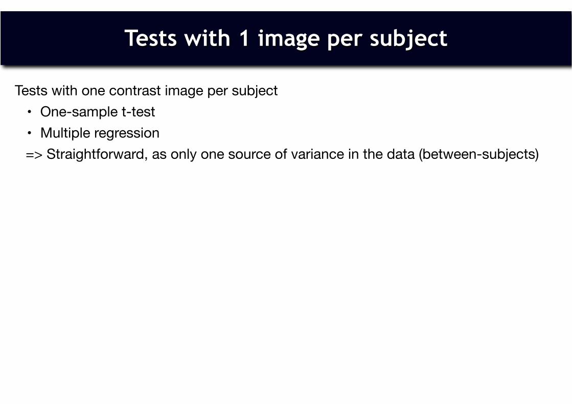
Tests with 1 image per subject

Tests with one contrast image per subject• One-sample t-test • Multiple regression

=> Straightforward, as only one source of variance in the data (between-subjects)

One-sample t-test

Is the mean of the data different from zero?

Multiple regression

Do the data correspond to numerical predictions for each image?

Tests with multiple groups /images per subject

Tests with multiple images per subject, or multiple groups • Two-sample and paired t-test • n-way ANOVA (between and within)• Full and flexible factorial=> More complicated: Several sources of variance and/or correlated values => See talk on group analyses

Tests with one contrast image per subject• One-sample t-test • Multiple regression

=> Straightforward, as only one source of variance in the data (between-subjects)

Two-sample t-test

Do the means of two independent sets of data differ? Example: Comparisons of patients and healthy controls

Paired t-test

Do the means of two dependent sets of data differ? Example: Pre-post designs with TMS or pharmacological interventions Note: Can also be tested with a one-sample t-test of the difference

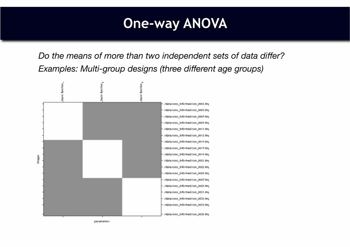
One-way ANOVA

Do the means of more than two independent sets of data differ? Examples: Multi-group designs (three different age groups)

One-way ANOVA - within subjects

Do the means of more than two dependent sets of data differ? Examples: Multi-intervention designs (baseline, intervention, baseline)

Factorial ANOVAs

ANOVAS can have several factors reflecting different, interacting experimental effects (e.g., 2x2 ANOVA)

SPM offers factorial designs that specify contrasts for main effects and interactionsThese estimate either all (full factorial) or specified (flexible factorial) effects

Note that within-subject main effects and interactions can also be tested with one-sample t-tests of the corresponding first-level contrasts(this is the “cleanest” way, as only source of variance is between-subject)

But sometimes it may be necessary/helpful to estimate ANOVA effects at 2nd level (e.g., mixed within/between designs, F-tests between any levels of factors)

Examples in the practical session on “group analyses”

Overview







Documents

Modelling of hemodynamic timeseries and 2nd-level … · Modelling of hemodynamic timeseries and 2nd-level summary statistics ... SPM(t) Data Design matrix ... Trial spacing • Design