Embed Size (px)
Citation preview

UNIVERSIDAD DE LAS AMÉRICAS PUEBLA
School of Engineering
Department of Industrial, Mechanical and Logistics Engineering
Modelling of a Rotary Hammer with the implementation of a Dynamic Eliminator of Vibrations
Thesis that the Student Presents to Complete the Requirements of the UDLAP
Honors Program
Roberto Sanz Camacho
ID: 150345
Bachelor’s in Mechanical Engineering
Dr. Tadeusz Majewski
San Andrés Cholula, Puebla. Fall 2018
2
Signature Sheet
Thesis that the Student Roberto Sanz Camacho ID: 150345 Presents to
Complete the Requirements of the Honors Program
Thesis Director
________________________
Dr. Tadeusz Majewski
Thesis President
_________________________
Dr. René Ledesma Alonso
Thesis Secretary
_________________________
Dr. Jorge Arturo Yescas Hernández
3
ACKNOWLEDGMENTS El presente trabajo es muestra del esfuerzo y la dedicación puesta en mis estudios a lo largo
de una de las mejores etapas de mi vida. Primero que nada, quiero agradecer a Dios por ser
mi guía y darme la fortaleza para salir adelante en cada una de las dificultades y problemas
de mi carrera.
También, quiero agradecer a mis padres por todo el apoyo que me han dado desde que soy
pequeño y por haberme dado la oportunidad de estudiar en esta universidad. Papá, muchas
gracias por enseñarme a ser quien soy y por ser mi ejemplo a seguir, gracias por enseñarme
a ser una persona honesta y trabajadora y por dar tu máximo esfuerzo para que nosotros
siempre tengamos lo mejor. Mamá, muchas gracias por estar ahí para mí las 24 horas del
día y 7 días de la semana, gracias por ser mi doctora y atender todas mis preocupaciones.
Carmen y Fer, gracias por estar siempre ahí para mí, compartir buenos momentos conmigo
y hacerme sonreír. Saben que siempre estaré para ustedes y nunca les fallaré.
Abuelos, muchas gracias por todas las historias y experiencias contadas, por las sonrisas y
el cariño que siempre me han mostrado, por mantener a nuestra familia siempre unida sin
importar la situación, he aprendido mucho de ustedes. A mis tíos y tías, por siempre estar
dispuestos a ayudarme. A mi novia María Fernanda, por aguantarme durante toda mi
carrera y hacerme tan feliz durante todos estos años.
De igual forma quiero agradecer a mis profesores y a esta institución por todas las
enseñanzas y por ser siempre receptivos a mis preguntas, que seguramente fueron muchas.
Especialmente quiero agradecer a mi amigo el Dr. Tadeusz por compartirme sus
conocimientos y su dedicación para sacar adelante este proyecto.
Finalmente, doy gracias a mis amigos tanto de la prepa como los que hice a lo largo del
camino, por hacer que estos 4 años y medio fueran inolvidables. Gracias a Andrés, Jesús,
Ricardo, Maus, Chapa, Gale, Belmont, Grecia, Quiroz, Sergio, Gabs, Chobo, Churro, Guru,
Chucho, Miguel, Juan, Adolfo, Pau, Yayo y Xotla; por hacer de esta etapa un recuerdo que
llevaré siempre conmigo. Muchas gracias a todos, no lo hubiera logrado sin ustedes.
4
“To give anything less than your best is to sacrifice the gift”
-Steve Prefontaine
5
CONTENTS
ACKNOWLEDGMENTS .................................................................................. 3
CONTENTS ....................................................................................................... 5
LIST OF FIGURES ............................................................................................ 8
LIST OF TABLES ........................................................................................... 11
ABSTRACT ..................................................................................................... 12
CHAPTER I – Introduction ............................................................................. 13
1.1 Context of the Research ......................................................................................... 13
1.2 Research Questions ................................................................................................ 14
1.3 Outline of the Document ........................................................................................ 14
CHAPTER II – Power Tools ............................................................................ 16
2.1 Introduction ................................................................................................................. 16
2.2 Power tools and their vibrations production ............................................................... 16
2.3 Impact tools and their working principles .................................................................. 19
2.3.1 Impact wrench ................................................................................................. 19
2.3.2 Jack hammer .................................................................................................... 20
2.3.3 Hammer drill .................................................................................................... 21
2.3.4 Rotary hammer ................................................................................................ 22
2.4 Vibrations effects on health ........................................................................................ 24
2.5 Damping systems for impact tools .............................................................................. 28
2.5.1 Makita Antivibration Technology ................................................................... 28
2.5.2 Dewalt Antivibration Technology ................................................................... 30
CHAPTER III – Dynamic Eliminator of Vibrations ....................................... 31
3.1 Introduction ................................................................................................................. 31
3.2 Frahm’s undamped dynamic vibration absorber......................................................... 31
3.3 Proposed Dynamic Eliminator of Vibrations .............................................................. 32
3.3.1 Matlab application ........................................................................................... 36
3.4 How this DEV works? - Inertial Force ....................................................................... 45
3.4.1 Inertial force solution with Matlab .................................................................. 48

6
CHAPTER IV – Rotary Hammer experiments and modelling ........................ 51
4.1 Introduction ................................................................................................................. 51
4.2 Experimental Set-up ................................................................................................... 51
4.2.1 Makita Rotary Hammer HR2511 ..................................................................... 51
4.2.2 Equipment for measuring vibrations ............................................................... 55
4.2.3 Makita rotary hammer experiments ................................................................. 57
4.3 Modelling of rotary hammer – Kinetic model with algebraic equations .................... 63
4.3.1 Matlab application ........................................................................................... 67
4.4 Modelling of rotary hammer – Dynamic model with differential equations .............. 71
4.4.1 Matlab application ........................................................................................... 74
CHAPTER V - Implementation of the Dynamic Eliminator of Vibrations to the Rotary Hammer .......................................................................................... 78
5.1 Introduction ................................................................................................................. 78
5.2 Mathematical modelling of rotary hammer with DEV analyzed in one direction (model with 2 drums and 4 spheres) ................................................................................. 78
5.2.1 Matlab application ........................................................................................... 81
5.3 Mathematical modelling of rotary hammer with DEV analyzed in two directions (model with 2 drums and 4 spheres) ................................................................................. 87
5.3.2 Matlab application ........................................................................................... 91
CHAPTER VI - Implementation of the DEV to the rotary hammer with the addition of the chisel chuck spring ................................................................... 99
6.1 Introduction ................................................................................................................. 99
6.2 Modelling of rotary hammer - Dynamic model with chisel chuck spring .................. 99
6.2.1 Matlab application ......................................................................................... 101
6.3 Mathematical modelling of rotary hammer with chisel spring connection and DEV implementation (2 directions, 2 drums, 4 spheres) ......................................................... 104
6.3.1 Matlab Application ........................................................................................ 105
CHAPTER VII - Conclusions ........................................................................ 110
7.1 Conclusions ............................................................................................................... 110
7.2 Future work ............................................................................................................... 111

7
APPENDICES ................................................................................................ 113
Appendix A - Matlab Codes ........................................................................................... 113
a) DEV with 2 free elements................................................................................ 113
b) DEV with 4 free elements................................................................................ 115
c) Inertial force..................................................................................................... 117
d) Kinetics description of the rotary hammer internal components ..................... 118
e) Dynamic model of rotary hammer behaviour .................................................. 121
f) Implementation of DEV to rotary hammer - unidirectional analysis .............. 124
g) Implementation of DEV to rotary hammer - bidirectional analysis ................ 128
h) Dynamic model of rotary hammer with chisel chuck spring ........................... 132
i) Implementation of DEV to the rotary hammer dynamic model with chuck spring ...................................................................................................................... 135
Appendix B - Matlab simulations ................................................................................... 140
Appendix C - Rotary hammer assembly diagram ........................................................... 142
REFERENCES ............................................................................................... 144
8
LIST OF FIGURES Figure 1. Impact wrench (Dahl, 2016) ................................................................................. 20 Figure 2. Impact wrench use (Dewalt, 2018) ....................................................................... 20 Figure 3. Jackhammer working principle (Woodford, 2018) ............................................... 21 Figure 4. Jackhammer use (2018)......................................................................................... 21 Figure 5. Hammer drill (Bosch, 2018) ................................................................................. 22 Figure 6. Hammer drill working principle (Family Handyman, 2018) ................................ 22 Figure 7. Rotary hammer working principle (Discovery, 2010) .......................................... 23 Figure 8. Rotary hammer components (Family Handyman, 2018) ...................................... 23 Figure 9. Rotary hammer application (Family Handyman, 2018) ....................................... 23 Figure 10. Coordinate system for measurement of complete-body vibrations (Majewski, 2017) ..................................................................................................................................... 24 Figure 11. Coordinate system for measurement of hand-arm vibrations (Majewski, 2017) 25 Figure 12. White finger syndrome (Ideara, 2014) ................................................................ 27 Figure 13. WFS effects (2014) ............................................................................................. 27 Figure 14. Makita AVT (Makita, 2018) ............................................................................... 28 Figure 15. Active-Dynamic Vibration absorber (2018) ....................................................... 29 Figure 16. Damper spring mechanism (Makita, 2015) ......................................................... 29 Figure 17. Floating handle (Dewalt, 2018) .......................................................................... 30 Figure 18. Floating handle components (2018) .................................................................... 30 Figure 19. Dewalt Active Vibration Control (2018) ............................................................ 30 Figure 20. Dewalt AVC components (2018) ........................................................................ 30 Figure 21. Undamped Dynamic Vibration Absorber (Rao, 2011) ....................................... 32 Figure 22. Proposed DEV ..................................................................................................... 33 Figure 23. Experiment 1 results (same initial position) ....................................................... 38 Figure 24. Experiment 1 equilibrium position ..................................................................... 39 Figure 25. Experiment 2 results (different initial position) .................................................. 40 Figure 26. Experiment 2 equilibrium position ..................................................................... 41 Figure 27. Experiment 3 results ........................................................................ 42 Figure 28. 4 spheres - DEV results ....................................................................................... 43 Figure 29. Experiment 4 equilibrium position ..................................................................... 44 Figure 30. Vibrations amplitude reduction for 4-element DEV ........................................... 44 Figure 31. Ideal results - 4 elements ..................................................................................... 44 Figure 32. Ideal equilibrium position - 4 elements ............................................................... 45 Figure 33. Inertial Force as function of α ............................................................................. 49 Figure 34. Makita HR2511 ................................................................................................... 52 Figure 35. HR2511 inside view ............................................................................................ 52 Figure 36. Top section of gearbox ........................................................................................ 53 Figure 37. Bottom section of gearbox .................................................................................. 53
9
Figure 38. Components description ...................................................................................... 53 Figure 39. Piston (front view) .............................................................................................. 53 Figure 40. Piston (top view) ................................................................................................. 53 Figure 41. Striker .................................................................................................................. 53 Figure 42. Transmission gear box ........................................................................................ 54 Figure 43. Tranmission gear box .......................................................................................... 54 Figure 44. Makita's rotary hammer cross section ................................................................. 54 Figure 45. Vibrations measuring equipment layout ............................................................. 56 Figure 46. Software parameters for sensing vibrations ........................................................ 56 Figure 47. Rotary hammer vibrations without impacts ........................................................ 57 Figure 48. Frequencies of vibration (without impacts) ........................................................ 57 Figure 49. Test samples ........................................................................................................ 58 Figure 50. Tests on asphalt (left) and concrete (right) ......................................................... 58 Figure 51. Hammer vibrations during impact with asphalt .................................................. 59 Figure 52. Frequencies of vibration for test on asphalt ........................................................ 59 Figure 53. Hammer vibrations during impact with concrete ................................................ 60 Figure 54. Frequencies of vibration for test on concrete ...................................................... 60 Figure 55. Brüel & Kjaer calibration exciter ........................................................................ 61 Figure 56. Vibrations produced by calibration exciter ......................................................... 61 Figure 57. Frequencies of vibration of calibration exciter ................................................... 61 Figure 58. Rotary hammer modelling................................................................................... 64 Figure 59. Striker (x) colliding with returning piston (z) ..................................................... 66 Figure 60. Experiment 1 (kinetic model) ............................................................................. 68 Figure 61. Experiment 2 (kinetic model) ............................................................................. 69 Figure 62. Experiment 3 (kinetic model) ............................................................................. 70 Figure 63. Rotary hammer model ......................................................................................... 72 Figure 64. Experiment 1 results (dynamic model) ............................................................... 75 Figure 65. Amplitude of vibration of hammer case.............................................................. 75 Figure 66. Impacts between chisel and floor ........................................................................ 76 Figure 67. Experiment 2 results (dynamic model) ............................................................... 76 Figure 68. Rotary Hammer with DEV.................................................................................. 79 Figure 69. Vibrations of the rotary hammer with 4-ball DEV ............................................. 83 Figure 70. Forces in rotary hammer with 4-ball DEV .......................................................... 84 Figure 71. Equilibrium position diagram for DEV............................................................... 84 Figure 72. Vibrations absorption .......................................................................................... 85 Figure 73. Vibrations of the chisel ....................................................................................... 85 Figure 74. Influence of increase in viscous damping coefficient. ........................................ 86 Figure 75. Influence of reduction in viscous damping coefficient. ...................................... 86 Figure 76. Rotary Hammer with DEV (XY analysis) .......................................................... 88 Figure 77. Vibrations in rotary hammer with 4-ball DEV ................................................... 94 Figure 78. Forces in rotary hammer with 4-ball DEV .......................................................... 94

10
Figure 79. Equilibrium position diagram for DEV............................................................... 95 Figure 80. Vibrations results with f=57.8 Hz ....................................................................... 96 Figure 81. Forces of the system with f=57.8 Hz .................................................................. 97 Figure 82. Equilibrium positions when f=57.8 Hz ............................................................... 97 Figure 83. System's optimization results .............................................................................. 98 Figure 84. Rotary hammer chuck. ........................................................................................ 99 Figure 85. Chuck spring. ...................................................................................................... 99 Figure 86. Rotary hammer with chuck spring .................................................................... 100 Figure 87. Rotary hammer vibrations (model with chuck spring) ..................................... 102 Figure 88. Rotary hammer forces ....................................................................................... 103 Figure 89. Rotary hammer with DEV and chuck spring .................................................... 104 Figure 90. Rotary hammer vibrations with chuck spring and 4-ball DEV ......................... 107 Figure 91. Forces produced by rotary hammer with chuck spring and 4-ball Dev ............ 107 Figure 92. Equilibrium position for model with chuck spring ........................................... 108 Figure 93. Vibrations of rotary hammer with DEV (ω=365 rad/s) .................................... 109 Figure 94. Rotary hammer forces with DEV (ω=365 rad/s) .............................................. 109 Figure 95. Experiment for cR=8 rad/s ................................................................................ 140 Figure 96. Experiment for cR=0.5 rad/s ............................................................................. 141

11
LIST OF TABLES
Table 1. Typical ranges of vibration for hand power tools (Ideara, 2014) ........................... 18 Table 2. Final position of free elements experiment 1 ......................................................... 39 Table 3. Final positions of free elements experiment 2 ........................................................ 40 Table 4. Final positions of free elements experiment 4 ........................................................ 43 Table 5. Rotary hammer main parameters ........................................................................... 54 Table 6. Makita rotary hammer dimensions ......................................................................... 55 Table 7. Period of vibration for impacts on asphalt ............................................................. 59 Table 8. Frequency of the 1st harmonic for exciter and hammer ......................................... 62 Table 9. Equilibrium position of free elements in DEV application to rotary hammer ....... 84 Table 10. Equilibrium position of free elements in DEV application to rotary hammer ..... 95 Table 11. Final position of the spheres (model with chuck spring) ................................... 108

12
ABSTRACT
The mathematical modelling of a Dynamic Eliminator of Vibrations is presented. This
model is based on two drums that rotate in opposite directions with a speed equal to the
excitation frequency of the system. These drums contain the same amount of free elements
such as rollers or spheres that translate in a viscous environment and compensate the
excitation forces with the action of their centrifugal force. Also, a rotary hammer working
principle is modelled with a novel method for the mathematical implementation of the DEV
to this system, to determine the possibility of vibrations damping. Several systems of
equations are developed and solved numerically using different input parameters. Results of
these simulations where vibrations reduction (of 99%) is illustrated, are presented
throughout this work, starting from simpler models up to systems with several degrees of
freedom.

13
CHAPTER I – Introduction
1.1 Context of the Research
Vibrations can exist in all the systems that are part of this planet. They are produced in a
great variety of conditions that define their intensity, duration, and frequency. These
conditions mainly depend on the characteristics of the system itself, the excitation source
and the way the vibrations are produced. This means that while some bodies could
experience stronger vibrations for a short amount of time, others could suffer imperceptible
vibrations for longer periods of time.
In most of the cases, vibrations are an undesirable phenomenon that affects different
systems. On the one hand, they can affect mechanical devices and structures, causing
fatigue damage, components wear and noise. On the other hand, the human body is harmed
by certain levels of vibration that can cause muscular and osteoarticular disorders. For that
reason, design engineers have spent great efforts in developing systems that can reduce
vibrations to an acceptable level.
One example of this situation is well described by the use of power tools in areas such as
construction, woodworking, manufacturing, among others, which produce high levels of
vibrations, directly affecting the user; even leading to permanent health issues.
Therefore, companies have developed specialized damping systems that absorb and try to
eliminate vibrations produced by power tools, particularly, impact ones. Examples of these
technologies have been developed by leading companies of this sector such as spring
mechanisms, floating handles, different types of active and dynamic vibration absorbers,
etc.

14
Hence, a Dynamic Eliminator of Vibrations is proposed in this work, based on the theory
developed by Dr. Tadeusz Majewski and with the purpose of determining its grade of
effectiveness in vibrations damping. This system is mathematically modelled and solved
with Matlab software. Additionally, the working principle of a rotary hammer is also
modelled with the purpose of evaluating the feasibility of the implementation of a DEV of
this kind.
1.2 Research Questions
During the definition of the general scope for this work, some questions arose and were
answered as one of the main objectives of this research.
I. Why is it so important to damp vibrations? Which are the main medical issues
caused by the exposure to high levels of vibration?
II. How does a Dynamic Eliminator of Vibrations work?
III. What is the working principle of a rotary hammer? How could it be modelled
mathematically?
IV. Is it possible to reduce vibrations produced by a rotary hammer with a Dynamic
Eliminator of Vibrations? Under which conditions is it possible to accomplish?
1.3 Outline of the Document
This work intends to develop the mathematical model of a Dynamic Eliminator of
Vibrations, as well as, explain the mechanics behind this system. In this thesis, the author
should determine whether it is possible or not to reduce vibrations produced by a device
such as a rotary hammer and under which circumstances this could be accomplished.

15
A rotary hammer has been chosen from a list of impact tools available for the research with
the purpose of having a real life reference and application.
Hence, this thesis is structured in several chapters that include the work done through this
entire project and the obtained results at each stage.
After setting the context in chapter I, a brief description of the most common power impact
tools and their working principle is given in chapter II; along with the explanation of the
vibrations effects on health and the existing damping systems and technologies for their
reduction.
Then, the Dynamic Eliminator of Vibrations is presented in chapter III, starting with a
simple model based on Lagrange Equations. Additionally, the mechanics of this system are
also explained in this section. Afterwards, in chapter IV, the description of the rotary
hammer chosen for this work is given. Some measurements of its vibrations production are
presented, as well as, two different approaches of the mathematical modelling of this
device. The first one is a kinetic model based on algebraic equations that describes the
motion of the main components of this system. Then, a dynamic model is proposed based
on differential equations with the objective of the further combination with the DEV
equations developed in chapter III.
The implementation of the DEV to the rotary hammer is described in chapter V, being
analyzed in one and two directions of motion. Finally, in chapter VI, a spring connection
between the main body and the chisel, is added to approximate the model to the real
complexity of the rotary hammer. This model is also analyzed with and without the
implementation of the DEV. It is important to mention that theory, equations and graphical
representation of models numerical solution in Matlab are combined throughout this work
in an organized manner that helps the reader understand the aims of this project.

16
CHAPTER II – Power Tools
2.1 Introduction
As explained earlier, this work is going to be focused on the application of a Dynamic
Eliminator of Vibrations on impact tools. Accordingly, this section starts with a brief
description of this kind of tools and the medical issues that the exposure to these systems
vibrations represent for the human body.
2.2 Power tools and their vibrations production
Tools are the means that allow man to do what he cannot do with his bare hands. A power
tool is a device that is actuated by an external source or mechanism, such as internal
combustion engines, electric motors, and compressed air; that allows the user to perform
tasks that he cannot easily do by himself. In particular, the AC motor represented a
breaking point for the evolution of power tools.
Tools can be classified in portable or hand tools (such as rotary hammer, drills, impact
wrench, etc.) and stationary power tools (e.g. bandsaw, lathe, disc sander, etc.). The main
advantage of hand tools is their mobility, whereas stationary tools can provide more
precision. A vast percentage of power tools transmit vibrations to the user through the
hand-arm system, which could have repercussion on his health (Ideara, 2014). These effects
will be discussed later.
Sectors of higher incidence of the usage of this type of tools include construction, metal-
mechanical, woodworking, automotive, and agricultural. For construction, there are
different types of tools from hand devices to big machines powered by combustion engines.
In this sector, pneumatic tools are also commonly used. The main tools used in construction
17
include jackhammer, rotary hammer drill, impact wrench, asphalt cutter, paving roller,
compactor, etc.
In the case of metal-mechanical area, there are stationary tools such as lathe, miter saw and
mill for metal machining and portable ones like disc cutter, drill, and grinder. For
woodworking, the most common power tools are polisher, disc saw, drill, and sander. For
the automotive sector, impact wrenches represent a very useful tool for changing lug nuts
and bolts. In agriculture, small combustion engines devices are used for the mechanization
of the processes. Some examples are lawn mower, brush cutter and motor hoe, among
others (Ideara, 2014).
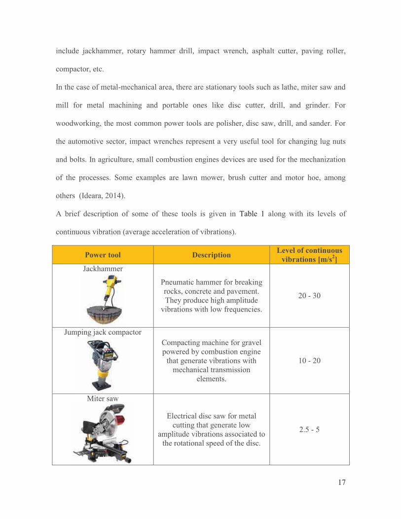
A brief description of some of these tools is given in Table 1 along with its levels of
continuous vibration (average acceleration of vibrations).
Power tool Description Level of continuous vibrations [m/s2]
Jackhammer
Pneumatic hammer for breaking rocks, concrete and pavement. They produce high amplitude
vibrations with low frequencies.
20 - 30
Jumping jack compactor
Compacting machine for gravel powered by combustion engine
that generate vibrations with mechanical transmission
elements.
10 - 20
Miter saw
Electrical disc saw for metal cutting that generate low
amplitude vibrations associated to the rotational speed of the disc.
2.5 - 5

18
Chainsaw
Portable, mechanical saw powered by a combustion engine. 5 - 12
Brush cutter
Agricultural tool used to trim grass, weeds and small trees in areas not accessible by a lawn mower. Powered by electrical motor or combustion engine.
2 - 23
Grinder/disc saw
Electrical hand tool for different usages such as cutting and
grinding depending on the type of disc mounted.
1 - 15
Hammer drill
Drill with hammering action that has two discs or gears that impact each other transmitting impacts to
the drill bit.
6 – 35
Rotary hammer
Powerful electric tool that pounds the drill bit in and out while
rotating with a piston-crankshaft mechanism.
5 – 24
Table 1. Typical ranges of vibration for hand power tools (Ideara, 2014)

19
2.3 Impact tools and their working principles
Particular attention is put to impact tools in this work. These tools include the impact
wrench, the rotary hammer, the hammer drill, the jackhammer, among others. The working
principle of each of these tools is described in this section, because of the special interest of
this research on impacts and vibrations production, and the effects they can produce on
human health.
2.3.1 Impact wrench
The impact wrench is a tool that provides a high amount of torque and allows bolts
installation and removal at very high speeds. The torque application is not constant, but
intermittent. Its working principle could be understood as a common wrench used to loosen
a screw or bolt, being hit by a hammer and making it turn gradually. When the impact
wrench is energized, an internal hammer strikes an anvil that is connected to a chuck
mandrel and the socket on the operating end of the tool. This commonly happens 2 times
per rotation. The hammer goes back and forth with a spring. This torque is transmitted to
the chuck and that rotation energy is used for loosen or tighten a nut, screw or bolt. This
mechanism allows the hammer to spin freely before and after impacting the anvil (Dahl,
2016). Internal parts of an impact wrench and an example of its use can be seen in Figure 1
and Figure 2, respectively.
The hammering effect is the characteristic that distinguishes this tool from conventional
drills, and allows the user to imprint a higher force than that generated with a common
wrench or ratchet. Additionally, this effect also helps to remove rust on the nut or bolt that
could make its extraction difficult. The power source of an impact gun can be electricity,

20
compressed air and even lithium batteries. These tools can provide torque from 100 to 700
lb·ft (from 120 N·m to 850 N·m) depending on the model with a breakaway point that
represents a security measure for applications that require excessive amount of torque; in
this case the hammering mechanism will be disengaged for preventing tool damage (Dahl,
2016).
Figure 1. Impact wrench (Dahl, 2016)
Figure 2. Impact wrench use (Dewalt,
2018)
2.3.2 Jack hammer
A Jackhammer is a powerful tool, pneumatically or electro-mechanically driven, used in
construction sites for breaking rock or pavement. There also exists a larger version that is
hydraulically powered. A jackhammer operates by moving an internal hammer up and
down transmitting the impacts to the chisel, producing 25 to 30 impacts per second
(Woodford, 2017).
As it is explained in Figure 3, the pneumatic jackhammer working principle is based on the
movement of a reciprocating valve that allows the sequential pass of compressed air in two
different directions, making a piston to go up and down, striking the drill bit repeatedly into
the ground. The valve’s main function is to regulate the air command and send it on either
one side or the other of the plunger or piston. Another basic component is the cylinder in

21
which the piston moves. This last component hits the head of the tool located at the lower
end of the hammer which transmits the impact to the ground, breaking it. The source of
power is an independent compressor, able to supply a volume of compressed air suitable to
the tool (Woodford, 2017)
The hydraulic version works with a (hydraulic) fluid instead of compressed air, at higher
pressures. This device is usually larger and is mounted on an excavator for operation.
Figure 4, shows an example of the use of a pneumatic jackhammer.
Figure 3. Jackhammer working principle (Woodford, 2017)
Figure 4. Jackhammer use (2017)
2.3.3 Hammer drill
A hammer drill is an electrical power tool used for hard surfaces drilling due to its
hammering action. This action can be understood as hitting the back of the drill with a
hammer. This mechanism allows it to break a surface more quickly and with less effort. Its
hammering mechanism is based on 2 splined discs or gears that rotate while contacting
each other. When this happens, the impacts and vibration waves are transmitted to the drill
22
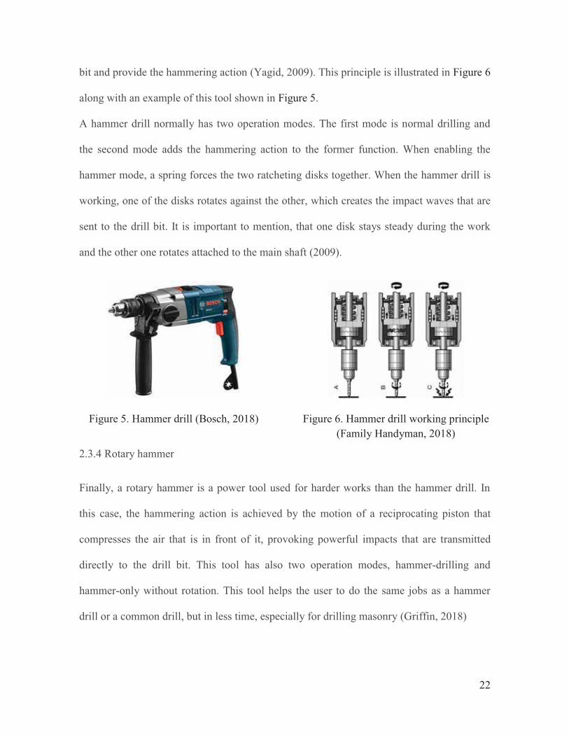
bit and provide the hammering action (Yagid, 2009). This principle is illustrated in Figure 6
along with an example of this tool shown in Figure 5.
A hammer drill normally has two operation modes. The first mode is normal drilling and
the second mode adds the hammering action to the former function. When enabling the
hammer mode, a spring forces the two ratcheting disks together. When the hammer drill is
working, one of the disks rotates against the other, which creates the impact waves that are
sent to the drill bit. It is important to mention, that one disk stays steady during the work
and the other one rotates attached to the main shaft (2009).
Figure 5. Hammer drill (Bosch, 2018)
Figure 6. Hammer drill working principle (Family Handyman, 2018)
2.3.4 Rotary hammer
Finally, a rotary hammer is a power tool used for harder works than the hammer drill. In
this case, the hammering action is achieved by the motion of a reciprocating piston that
compresses the air that is in front of it, provoking powerful impacts that are transmitted
directly to the drill bit. This tool has also two operation modes, hammer-drilling and
hammer-only without rotation. This tool helps the user to do the same jobs as a hammer
drill or a common drill, but in less time, especially for drilling masonry (Griffin, 2018)
23
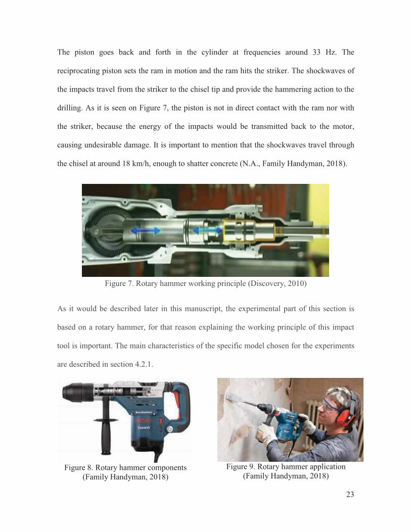
The piston goes back and forth in the cylinder at frequencies around 33 Hz. The
reciprocating piston sets the ram in motion and the ram hits the striker. The shockwaves of
the impacts travel from the striker to the chisel tip and provide the hammering action to the
drilling. As it is seen on Figure 7, the piston is not in direct contact with the ram nor with
the striker, because the energy of the impacts would be transmitted back to the motor,
causing undesirable damage. It is important to mention that the shockwaves travel through
the chisel at around 18 km/h, enough to shatter concrete (N.A., Family Handyman, 2018).
Figure 7. Rotary hammer working principle (Discovery, 2010)
As it would be described later in this manuscript, the experimental part of this section is
based on a rotary hammer, for that reason explaining the working principle of this impact
tool is important. The main characteristics of the specific model chosen for the experiments
are described in section 4.2.1.
Figure 8. Rotary hammer components
(Family Handyman, 2018)
Figure 9. Rotary hammer application
(Family Handyman, 2018)
24
2.4 Vibrations effects on health
Vibration is understood as any oscillatory movement of a body with respect to an
equilibrium position that is transmitted through a medium. When vibrations are intense,
they could have harmful effects on human’s health. The severity of the threat to health
depends on the frequency of vibration, time of exposure, intensity of the phenomenon and
its path into the human body (Hernández, 2012)
It is important to mention that vibrations are determined by their amplitude and frequency.
The amplitude of vibrations is usually measured with its acceleration (m/s2 or dB), whereas
the frequency is measured in hertz (Hz). The acceleration decibel is defined by:
(2.1)
Where a0 is a reference acceleration equal to 10-6 m/s2 (ISO 1683).
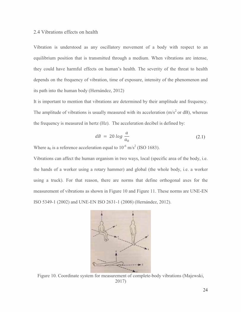
Vibrations can affect the human organism in two ways, local (specific area of the body, i.e.
the hands of a worker using a rotary hammer) and global (the whole body, i.e. a worker
using a truck). For that reason, there are norms that define orthogonal axes for the
measurement of vibrations as shown in Figure 10 and Figure 11. These norms are UNE-EN
ISO 5349-1 (2002) and UNE-EN ISO 2631-1 (2008) (Hernández, 2012).
Figure 10. Coordinate system for measurement of complete-body vibrations (Majewski,
2017)

25
Figure 11. Coordinate system for measurement of hand-arm vibrations (Majewski, 2017)
Particularly, rotary and impact tools produce high levels of vibrations. Therefore, the
constant use of this type of tools in sectors like industry, forestry and construction along
with other activities where vibrations exposure is repetitively experienced, can cause
medical issues like neck pain, headaches, dizziness, and other diseases (i.e. carpal tunnel
syndrome and Raynaud phenomenon) (Castro, Palacios, García, & Moreno, 2014).
The grade of affection to the human body produced by vibrations is determined by external
and internal factors. The external factors depend on the oscillatory movement itself, i.e.
frequency and amplitude of vibrations, point of application, direction, and working method.
Tool characteristics such as weight, equilibrium and supports are also considered an
external factor. Internal factors are those related to the user itself, i.e. its physique, weight,
working posture, health conditions, etc. (Hernández, 2012).
Vibrations produced by power tools and industrial equipment do not have a fixed
frequency; they are a superposition of vibrations with different frequencies. As it was
already mentioned the frequencies of interest for industrial safety vary from 1 to 1500 Hz.
Within this range, there are different effects of vibrations produced at different frequencies.
When the frequency is below 3 Hz, the human body moves as a rigid unit; at these
frequencies the main adverse effect is dizziness. As the frequency of vibration increases the
body parts tend to respond to the fluctuating forces in different ways. When the frequency

26
goes from 4 to 12 Hz, abdominal parts and shoulders start to vibrate amplifying the body’s
response to vibration. When the frequency reaches 20 Hz, the skull begins to vibrate
affecting visibility. After going higher than 60 Hz, the eyeballs tend to resonate with the
vibrating forces. The frequency of the power tools such as sanders, chainsaws and impact
tools varies from 20 to 1000 Hz (Ideara, 2014). The mentioned effects can be understood as
short term ones because they are an immediate response to the presence of vibrations and
they disappear gradually when the source of vibrations is removed.
However, there are long term effects that are produced by the continuous usage of devices
that transmit high levels of vibrations to the body, mainly through the hand-arm system;
resulting in muscular, osteoarticular, neurological and vascular disorders (Hernández,
2012). The muscular disorders are those injuries that affect muscles, joints and tendons.
These are associated with pain and discomfort, in addition to soreness and strength loss.
Moreover, loss of mobility can also be a consequence. Also, tendinitis or Dupuytren
contracture can occur. The Dupuytren contracture affects the palm connecting tissues that
produce the retraction of one finger, commonly the fourth or fifth one (Hernández, 2012).
Also, the long term exposure to complete body vibrations can affect the spinal column of
the worker, causing a degenerative alteration of the vertebrae and intervertebral discs
(Castro, Palacios, García, & Moreno, 2014).
Moreover, the osteoarticular disorders affect elbow articulation, shoulder, wrist and carpal
bones. On the one hand, elbow arthrosis produced by the use of percussion tools is
characterized by an intense pain suffered in the elbow area, that does not allow the worker
to continue on duty for several weeks. On the other hand, Kienböck’s disease is related to
the carpal bones, associated with pain and loss of mobility and gripping strength. Disorders
with osteoarticular origin are irreversible (Ideara, 2014).

27
The neurological disorders produced by vibratory tools include the loss of sensibility and
numbness of hands and fingers. This could result in the worker’s loss of ability to perform
precision tasks. In the vascular category, particular attention is put to the Vibration-induced
white finger syndrome (VWF), or Raynaud's phenomenon; caused by the continuous
exposure of the hand-arm system to intense vibrations.
Raynaud’s syndrome main characteristic is the intermittent whitening of one or more
fingers produced by the affectation to the hand nerves and joints. Specifically, it affects the
blood flow (vascular effect) and causes loss of touch sensation (neurological effect) in
fingers (Ideara, 2014).
Figure 12. White finger syndrome (Ideara, 2014)
Figure 13. WFS effects (2014)
In addition to that, there are other general disorders that not only affect the hand-arm
system. In these cases, vibrations are transmitted from hands to other parts of the body
depending on the type of vibration, its frequency and mainly the posture of the person. The
most common ailments of this kind are lumbar pain and hearing impairment. Lumbar pain
can be caused by degenerative changes like displacement of lumbar discs. “With regarding
to hearing, the human threshold can be displaced from 3 to 8 kHz if the weighted

28
acceleration exceeds an effective value of 1.2 m/s2 with simultaneous exposure to noise, at
a level equivalent to 80 dBA” (Ideara, 2014, p. 49).
2.5 Damping systems for impact tools
After the description of the health risks that the use of impact tools can produce, it is
important to mention the different kinds of damping systems that have been developed by
leading companies of this sector. Companies like Makita, Bosch and Dewalt have designed
their own mechanisms that absorb, reduce or dissipate the vibrations produced by power
tools in order to prevent user’s health disorders. Some of these systems and their working
principles will be described in this section.
2.5.1 Makita Antivibration Technology
Makita, the Japanese manufacturer of power tools, has developed an antivibrations system
known as AVT. This technology is based on 3 different vibrations damping mechanisms
which are the Active-Dynamic Vibration Absorber, a vibration absorbing housing and a
damper spring; all of them illustrated in Figure 14.
Figure 14. Makita AVT (Makita UK, 2018)
Damper spring
Active-Dynamic Vibration
Vibration absorbing grip
29
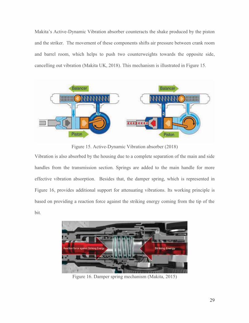
Makita’s Active-Dynamic Vibration absorber counteracts the shake produced by the piston
and the striker. The movement of these components shifts air pressure between crank room
and barrel room, which helps to push two counterweights towards the opposite side,
cancelling out vibration (Makita UK, 2018). This mechanism is illustrated in Figure 15.
Figure 15. Active-Dynamic Vibration absorber (2018)
Vibration is also absorbed by the housing due to a complete separation of the main and side
handles from the transmission section. Springs are added to the main handle for more
effective vibration absorption. Besides that, the damper spring, which is represented in
Figure 16, provides additional support for attenuating vibrations. Its working principle is
based on providing a reaction force against the striking energy coming from the tip of the
bit.
Figure 16. Damper spring mechanism (Makita, 2015)
30
2.5.2 Dewalt Antivibration Technology
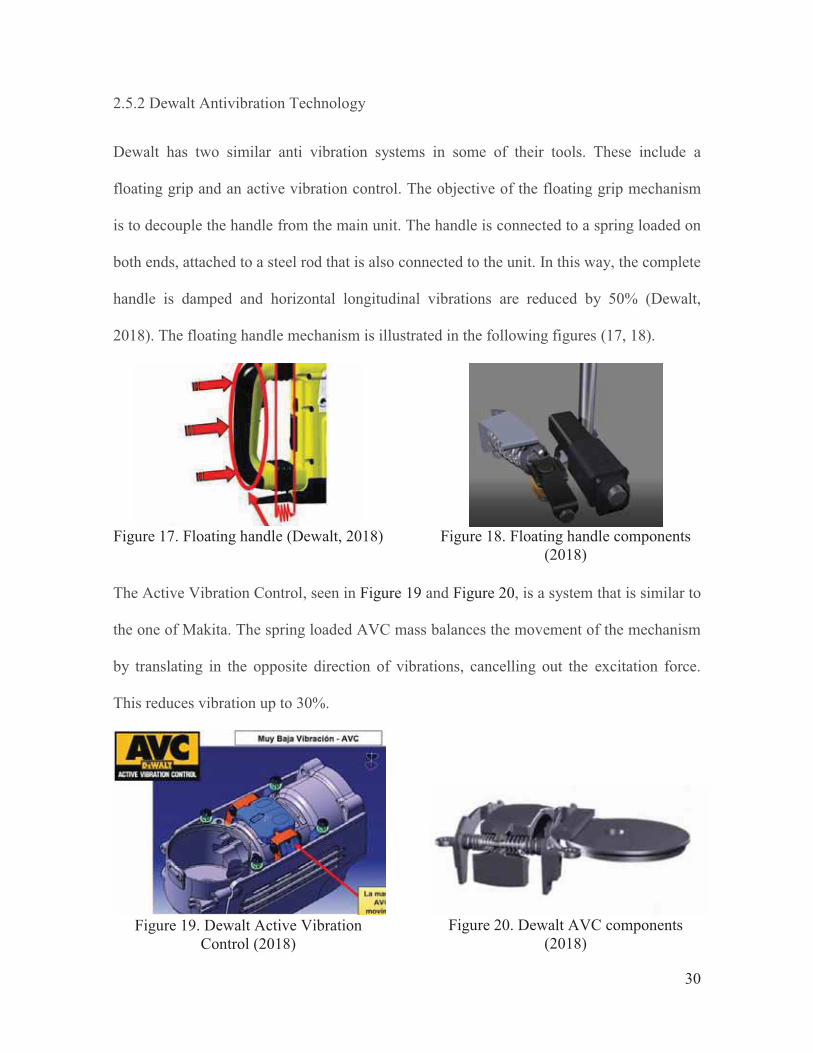
Dewalt has two similar anti vibration systems in some of their tools. These include a
floating grip and an active vibration control. The objective of the floating grip mechanism
is to decouple the handle from the main unit. The handle is connected to a spring loaded on
both ends, attached to a steel rod that is also connected to the unit. In this way, the complete
handle is damped and horizontal longitudinal vibrations are reduced by 50% (Dewalt,
2018). The floating handle mechanism is illustrated in the following figures (17, 18).
Figure 17. Floating handle (Dewalt, 2018)
Figure 18. Floating handle components
(2018)
The Active Vibration Control, seen in Figure 19 and Figure 20, is a system that is similar to
the one of Makita. The spring loaded AVC mass balances the movement of the mechanism
by translating in the opposite direction of vibrations, cancelling out the excitation force.
This reduces vibration up to 30%.
Figure 19. Dewalt Active Vibration
Control (2018)
Figure 20. Dewalt AVC components
(2018)

31
CHAPTER III – Dynamic Eliminator of Vibrations
3.1 Introduction
In this chapter, the theory behind a Dynamic Eliminator of Vibrations is explained. Also, a
DEV model with two rotary drums with free elements inside is proposed and described.
Governing equations of the system are established and they are solved with Matlab for
certain input parameters.
3.2 Frahm’s undamped dynamic vibration absorber
The DEV also called Dynamic Vibrations Absorber was first proposed by Hermann Frahm
about a century ago. Frahm’s undamped dynamic vibration absorber demonstrates that the
magnitude of a system’s response to an excitation can be reduced if an auxiliary mass,
called vibration absorber, is attached to the main body and the natural frequency of this
subsystem is equal or very similar to the frequency of excitation (Majewski, 2017)
In words of Jens T. Broch, a DEV is defined as that of “attaching to a vibrating structure a
resonance system which counteracts the original vibrations. Ideally, such a system would
completely eliminate the vibrations of a structure, in account of its own vibrations” (1972).
Thus, the main mass and the absorber, seen in Figure 21, constitute a two-degree-of-
freedom system with two natural frequencies. There are two main parameters that can be
selected in the design of a DEV for tuning the performance of the absorber: mass and
stiffness. M and k are selected with the purpose of making the natural frequency of the
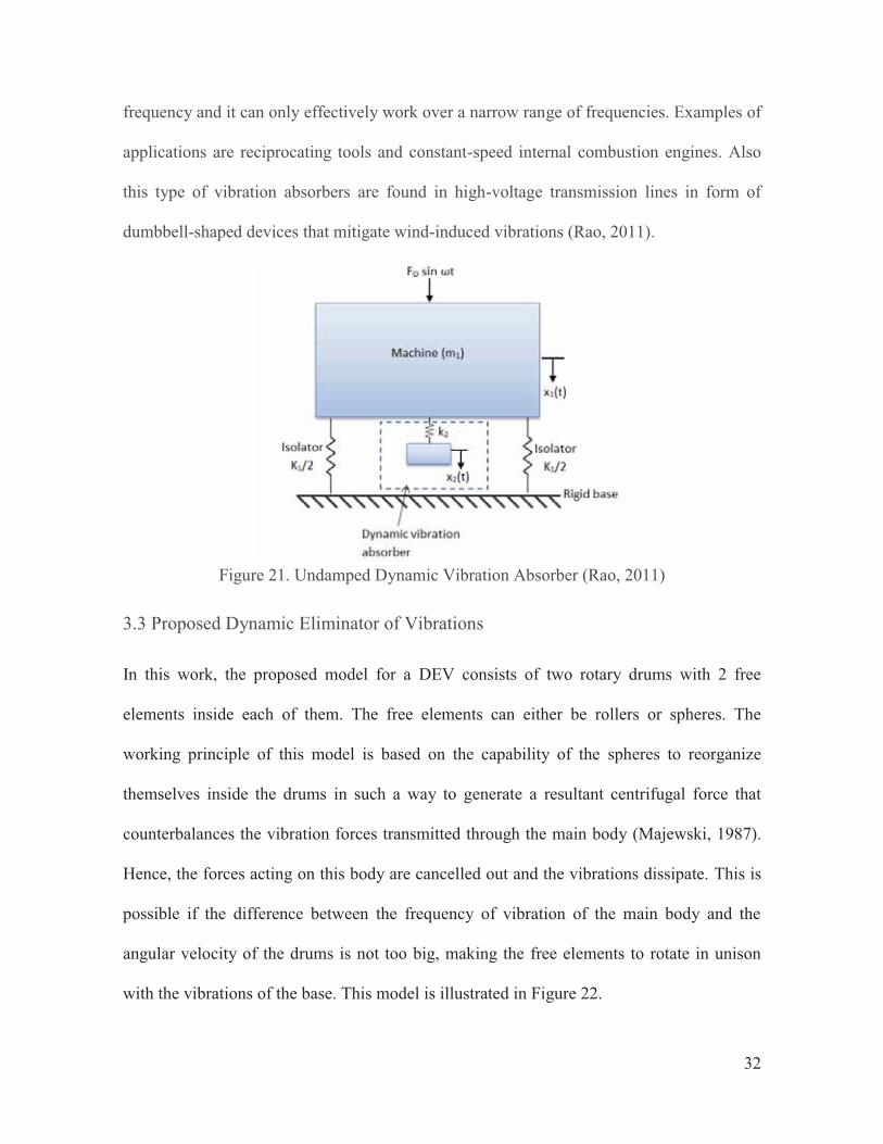
subsystem equal to the excitation frequency, that is to say: (Rao, 2011).
This principle is commonly used for machinery that operates at constant speed or for
systems with a major frequency component because the DEV is tuned to a particular
32
frequency and it can only effectively work over a narrow range of frequencies. Examples of
applications are reciprocating tools and constant-speed internal combustion engines. Also
this type of vibration absorbers are found in high-voltage transmission lines in form of
dumbbell-shaped devices that mitigate wind-induced vibrations (Rao, 2011).
Figure 21. Undamped Dynamic Vibration Absorber (Rao, 2011)
3.3 Proposed Dynamic Eliminator of Vibrations
In this work, the proposed model for a DEV consists of two rotary drums with 2 free
elements inside each of them. The free elements can either be rollers or spheres. The
working principle of this model is based on the capability of the spheres to reorganize
themselves inside the drums in such a way to generate a resultant centrifugal force that
counterbalances the vibration forces transmitted through the main body (Majewski, 1987).
Hence, the forces acting on this body are cancelled out and the vibrations dissipate. This is
possible if the difference between the frequency of vibration of the main body and the
angular velocity of the drums is not too big, making the free elements to rotate in unison
with the vibrations of the base. This model is illustrated in Figure 22.

33
Figure 22. Proposed DEV
Where, R, is the radius of the drum r, is the radius of the sphere k, is the stiffness of the spring c, is the damping coefficient of the system
, is the frequency of excitation equal to the rotary speed of the drums , is the phase angle of i-th free element with respect to the vertical axis , is the relative angular velocity of the i-th free element with respect to the drum
, is the velocity of the main body in vertical direction, is the external excitation of the system
As it can be seen in this initial model, the displacement of the main body is only allowed in
the vertical direction, named as “x”.
The model is solved using Lagrange equations; for this purpose, the resultant velocity of
the free bodies is needed and it is found using its x and y components.
y

34
Kinetic and potential energy are used as defined by Lagrange:
(3.1)
Where, , represents the generalized coordinates , represents the generalized velocities , is the kinetic energy of the system , is the potential energy of the system , represents generalized non-conservative forces
Kinetic energy:
(3.2)
Where, , is the mass of the main body. , is the mass of the spheres.
, is the mass moment of inertia of the spheres.
Potential energy due to the spring:
(3.3)
Non-conservative forces due to damping are obtained from virtual work equation (
):
Where cr, is the coefficient of viscous resistance for the free elements.
Therefore,
(3.4)

35
(3.5)
The derivatives of the kinetic and potential energy are obtained and the results are
substituted in the Lagrange equation:
(3.6)
Where , is the number of free elements.
(3.7)
The system is then solved for and . is substituted with
(3.8)
(3.9)
Where , is the equivalent mass of the
system.
A change of variable is done, where the term is substituted by the dimensionless time
variable τ for simplicity of the equations. The expressions obtained are:

36
(3.10)
(3.11)
The expression for centrifugal force can be used to determine the optimal mass of the free
elements because with this reaction the excitation force is cancelled out.
(3.12)
Additionally, the natural frequency of the system is determined by:
(3.13)
3.3.1 Matlab application
The obtained system of equations for the model is solved using Matlab due to its
complexity. Matlab function ode45 is used for this purpose. In order to utilize this function,
the system needs to be transformed into a system of 1st order differential equations.
First, the independent degrees of freedom are listed as follows for a DEV model of 4 free
elements, two inside each drum:
37
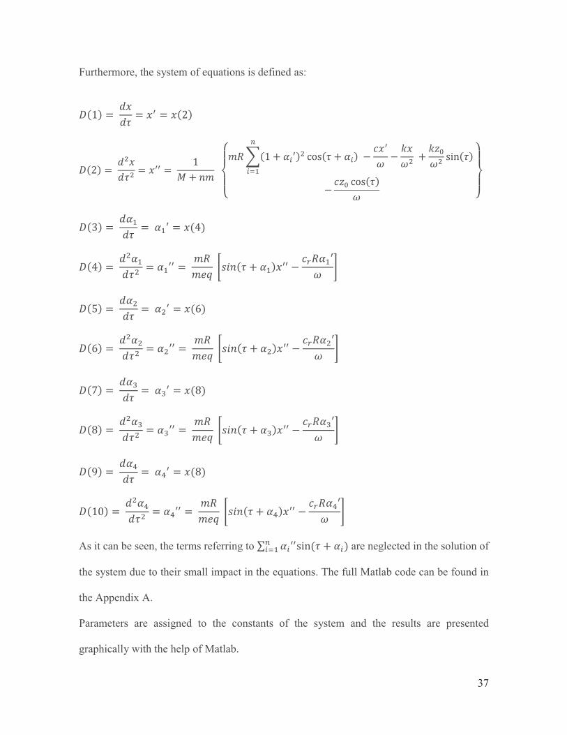
Furthermore, the system of equations is defined as:
As it can be seen, the terms referring to are neglected in the solution of
the system due to their small impact in the equations. The full Matlab code can be found in
the Appendix A.
Parameters are assigned to the constants of the system and the results are presented
graphically with the help of Matlab.

38
� Experiment 3.1: 1 sphere per drum, same initial position for both spheres
Parameters:
n = 3 Degrees of Freedom, ω = 100 rad/s, M = 4 kg, m = 0.054 kg, R = 0.05 m, r = 0.01
mm, c = 20 kg/s, cr=4 rad/s, k = 5000 N/m, z0 = 0.01 m
With 2 spheres and external excitation defined as
Initial conditions:
Figure 23. Experiment 1 results (same initial position)
The plots show that vibrations are damped from 7.2 mm of amplitude to 0.01 mm in 4
seconds. Reduction is around 720 times compared to the initial amplitude. Actually, in this

39
case, two curves are plotted for and but, as they start from the same position, they
follow the same path towards the equilibrium position.
The equilibrium positions found by the free elements are:
Final position of free elements Left drum Right drum
α2 3.5179 rad 201.6°
α1 3.5179 rad 201.6°
Table 2. Final position of free elements experiment 1
Figure 24. Experiment 1 equilibrium position
� Experiment 3.2: 1 sphere per drum, different initial position for both spheres
If the initial position of the balls is not the same , the system
is still balanced; however, it is more difficult for the free elements to achieve the same final
position which could make their location to be slightly asymmetric.

40
Figure 25. Experiment 2 results (different initial position)
The plots show that vibrations are damped from 3.1 mm of amplitude to 0.01 mm in 4
seconds. Reduction is around 300 times of initial amplitude of vibration.
The final positions of the free elements are:
Final position of free elements Left drum Right drum
α2 -2.881 rad -165.07°
α1 3.6404 rad 208.6°
Table 3. Final positions of free elements experiment 2
.
.

41
Figure 26. Experiment 2 equilibrium position
� Experiment 3.3: 1 sphere per drum, same initial position,
It is important to mention that the Dynamic Eliminator of Vibrations only works effectively
for frequencies that are over the natural frequency of the system. If the excitation frequency
is smaller than the natural frequency of the system, the free elements of the DEV enlarge
the vibrations amplitude instead of attenuating them.
An example of this phenomenon is showed in Figure 27, where the excitation frequency
and angular velocity of the drums (same value) are below the natural frequency of the
system and very close to resonance.
Frequency of excitation
42
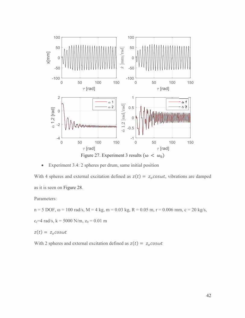
Figure 27. Experiment 3 results
� Experiment 3.4: 2 spheres per drum, same initial position
With 4 spheres and external excitation defined as , vibrations are damped
as it is seen on Figure 28.
Parameters:
n = 5 DOF, ω = 100 rad/s, M = 4 kg, m = 0.03 kg, R = 0.05 m, r = 0.006 mm, c = 20 kg/s,
cr=4 rad/s, k = 5000 N/m, z0 = 0.01 m
With 2 spheres and external excitation defined as
.
.

43
Figure 28. 4 spheres - DEV results
α1 and α3 are plotted in black and α2 and α4 in red. Final position of free elements is
registered to confirm that an equilibrium position for damping vibrations in vertical
direction is found.
Final position of free elements Left drum Right drum
α3 3.0736 rad 176.104°
α1 3.0736 rad 176.104°
α4 3.9727 rad 227.619°
α2 3.9727 rad 227.619°
Table 4. Final positions of free elements experiment 4

44
Figure 29. Experiment 4 equilibrium position
Amplitude of vibration is reduced from 6.6 mm to 0.001 mm. Reduction is more than 3000 times compared to the initial condition. This can be observed in
Figure 30, where a zoom of the final part of Figure 28 (x vs τ) is presented.
Figure 30. Vibrations amplitude reduction for 4-element DEV
If mass used is exactly 0.027 kg. The free elements position overlays because they try to
balance the system in the same way it was done with just 2 elements.
Figure 31. Ideal results - 4 elements

45
Figure 32. Ideal equilibrium position - 4 elements
3.4 How this DEV works? - Inertial Force
The diagrams and plots presented show how the free elements inside the drums eliminate
the object vibrations. Their final positions are opposite to the excitation of the system and
this allows them to counteract the produced vibrations.
This phenomenon happens as a result of the inertial force. Due to the action of this force,
the free elements move synchronically with the excitation and at some point they found the
equilibrium positions where the system stabilizes and the object stops vibrating. Therefore,
the working principle of this model of Dynamic Eliminator of Vibrations is based on the
existence and action of this inertial force.
The action of the inertial force and its impact in the equilibrium position of the free
elements can be better explained with the following equations. This model is only
developed in the vertical direction, just as illustrative principle of the DEV.
The governing equation for the main body in the system presented in Figure 22 has a
general shape of:
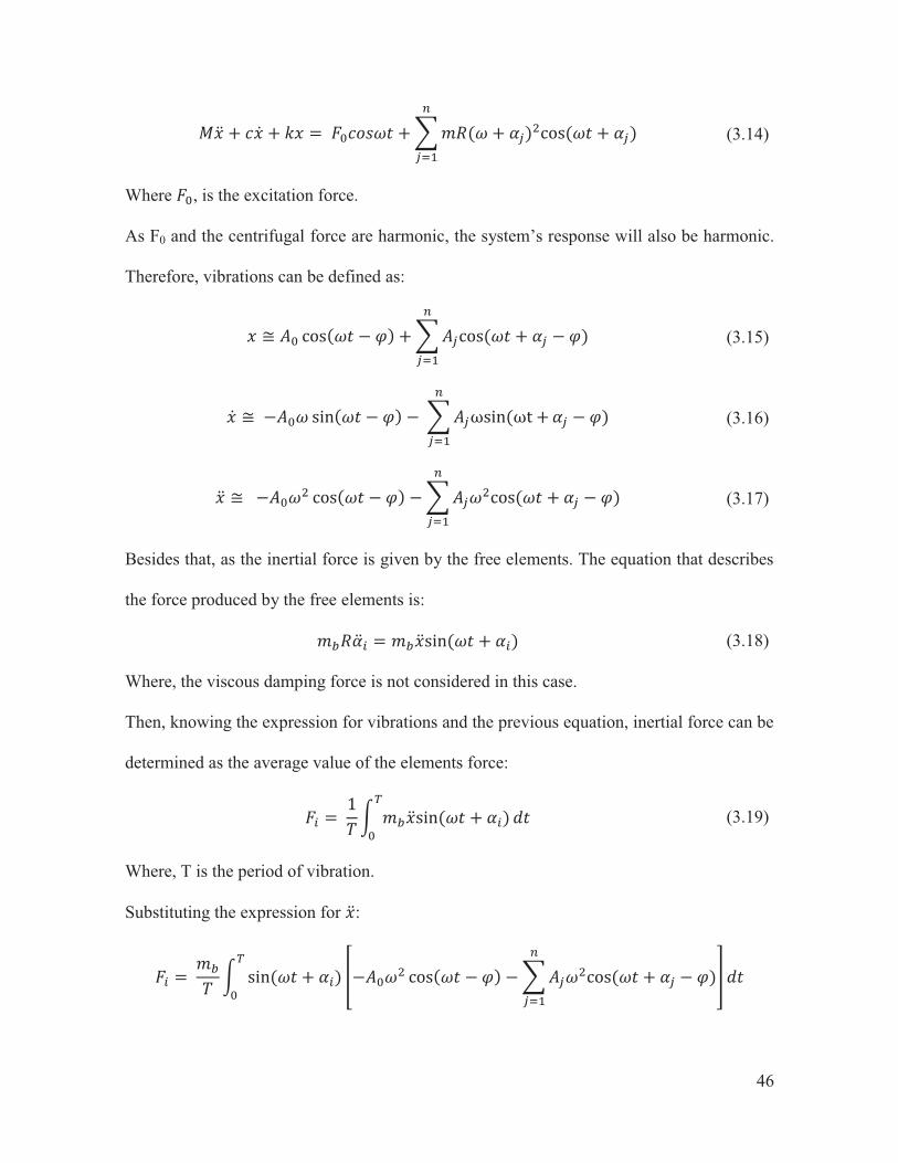
46
(3.14)
Where , is the excitation force.
As F0 and the centrifugal force are harmonic, the system’s response will also be harmonic.
Therefore, vibrations can be defined as:
(3.15)
(3.16)
(3.17)
Besides that, as the inertial force is given by the free elements. The equation that describes
the force produced by the free elements is:
(3.18)
Where, the viscous damping force is not considered in this case.
Then, knowing the expression for vibrations and the previous equation, inertial force can be
determined as the average value of the elements force:
(3.19)
Where, T is the period of vibration.
Substituting the expression for :
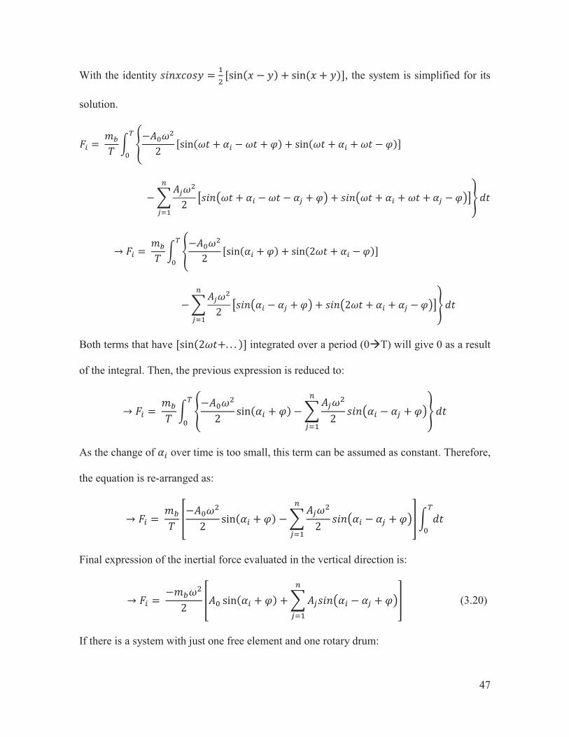
47
With the identity , the system is simplified for its
solution.
Both terms that have integrated over a period (0�T) will give 0 as a result
of the integral. Then, the previous expression is reduced to:
As the change of over time is too small, this term can be assumed as constant. Therefore,
the equation is re-arranged as:
Final expression of the inertial force evaluated in the vertical direction is:
(3.20)
If there is a system with just one free element and one rotary drum:

48
1 sphere and j only goes from 1 to 1. Therefore, . The previous equation can
be expressed as:
(3.21)
Also, as there is only one sphere, the amplitude of its response must be equal to the
amplitude of excitation in order to damp vibrations ( .
(3.22)
With the phase angle being defined as:
(3.23)
Where, depend on the system configuration and refer to the damping
coefficients and the stiffness of the springs respectively. M represents the mass of the main
body and ω the frequency of excitation.
These equations are input to Matlab and graphic solution is obtained.
3.4.1 Inertial force solution with Matlab
For easier computation of inertial force, the expression (3.22) is defined as:
(3.24)
Equations are coded in Matlab and the following parameters are assigned to the system:
M=4.175 kg, c1=10 kg/s, c2=10 kg/s, k1=10000 N/m, k2=10000 N/m and ω=100 rad/s.
49
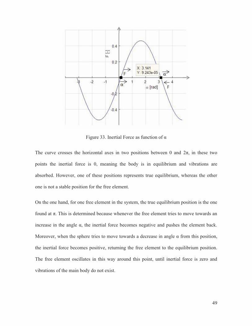
Figure 33. Inertial Force as function of α
The curve crosses the horizontal axes in two positions between 0 and 2π, in these two
points the inertial force is 0, meaning the body is in equilibrium and vibrations are
absorbed. However, one of these positions represents true equilibrium, whereas the other
one is not a stable position for the free element.
On the one hand, for one free element in the system, the true equilibrium position is the one
found at π. This is determined because whenever the free element tries to move towards an
increase in the angle α, the inertial force becomes negative and pushes the element back.
Moreover, when the sphere tries to move towards a decrease in angle α from this position,
the inertial force becomes positive, returning the free element to the equilibrium position.
The free element oscillates in this way around this point, until inertial force is zero and
vibrations of the main body do not exist.

50
On the other hand, if the free element is located at the position close to α=0, when it moves
towards an increase in alpha, the inertial force becomes positive and helps the sphere to
escape from this position. Same applies when the sphere moves towards negative alpha and
the inertial force helps it to move away.
Hence, this section explains how the free elements inside the drums are able to find and
stay in an equilibrium position, in which they are able to counteract the excitation forces
and eliminate vibrations.
Moreover, this kind of Dynamic Eliminator of Vibrations is modelled as part of a rotary
hammer system in order to determine the feasibility of implementation to this impact tool.
First, the rotary hammer working principle is modelled in sections 4.3 and 4.4 of this
document and then in chapter 5 models are brought up together
51
CHAPTER IV – Rotary Hammer experiments and modelling
4.1 Introduction
An impact tool was chosen with the intention to develop a mathematical model of the
Dynamic Eliminator of Vibrations based on real data of the vibrations produced by this
device. Hence, with the use of a real device and the experimental measurement of
vibrations amplitude and frequency, the results and damping capability of the EDV could
be determined accurately.
4.2 Experimental Set-up
The experiments and models developed in this work were based on the Makita Rotary
Hammer HR2511. This tool’s characteristics are provided in the following section along
with a more detailed description of its design and its working principle. For developing the
mathematical model of the EDV, it is also important to determine how impacts are
produced by this tool.
4.2.1 Makita Rotary Hammer HR2511
The Makita HR2511 is a rotary hammer featuring a 2 mode function to fulfill different
drilling applications. As any other rotary hammer it has a drilling function with pounding
action and a “hammering-only” one. This device, shown in Figure 34, has a net weight of
4.25 kg and an overall length of 370 mm. It has the capacity of drilling wood, steel and
concrete; being this last one its main application.
52
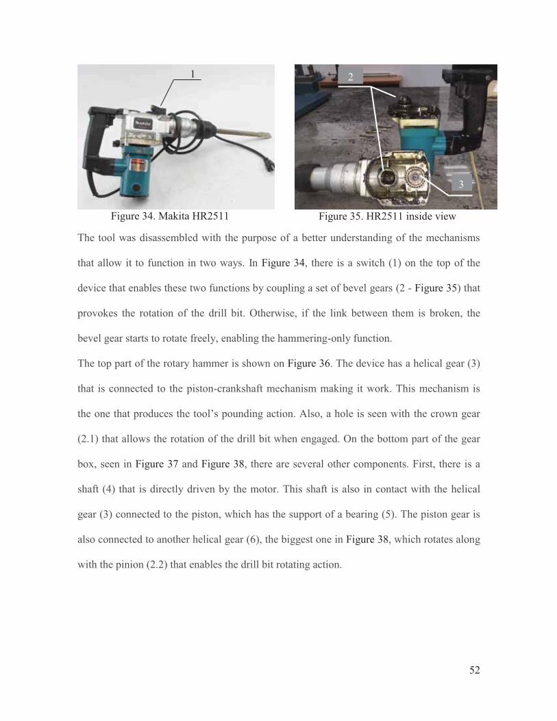
Figure 34. Makita HR2511
Figure 35. HR2511 inside view
The tool was disassembled with the purpose of a better understanding of the mechanisms
that allow it to function in two ways. In Figure 34, there is a switch (1) on the top of the
device that enables these two functions by coupling a set of bevel gears (2 - Figure 35) that
provokes the rotation of the drill bit. Otherwise, if the link between them is broken, the
bevel gear starts to rotate freely, enabling the hammering-only function.
The top part of the rotary hammer is shown on Figure 36. The device has a helical gear (3)
that is connected to the piston-crankshaft mechanism making it work. This mechanism is
the one that produces the tool’s pounding action. Also, a hole is seen with the crown gear
(2.1) that allows the rotation of the drill bit when engaged. On the bottom part of the gear
box, seen in Figure 37 and Figure 38, there are several other components. First, there is a
shaft (4) that is directly driven by the motor. This shaft is also in contact with the helical
gear (3) connected to the piston, which has the support of a bearing (5). The piston gear is
also connected to another helical gear (6), the biggest one in Figure 38, which rotates along
with the pinion (2.2) that enables the drill bit rotating action.
1 2
3

53
Figure 36. Top section of gearbox
Figure 37. Bottom section of gearbox
Figure 38. Components description
Inside the hammer cylinder, there is an air chamber with a striker inside. For the
hammering-only mode, this striker is not directly hit by the piston but moved by the air
compression in the chamber. After air is compressed the striker hits the chisel. The
shockwaves of each impact travel from the striker to the tip of the chisel. Piston and striker
can be observed in Figure 39 and Figure 41, respectively.
Figure 39. Piston (front
view)
Figure 40. Piston (top view)
Figure 41. Striker
4
2.2
3 2.1
5
6
2.2 5
6

54
In figures 42-44, components can be better appreciated with more detailed pictures and a
cross section of a similar device (in this case the bevel gear (6) is in direct contact with the
motor shaft (4), contrary to what it was described before).
Figure 42. Transmission gear box
Figure 43. Tranmission gear box
Figure 44. Makita's rotary hammer cross section
In the Table 5, the main parameters of the rotary hammer are presented. A detailed parts
diagram of this rotary hammer is shown in the Appendix section of this document.
Makita Rotary hammer
Voltage 120 v Frequency 60 Hz
Power 1.3 HP or 850 W Engine RPM 800-900 rpm
Blows per minute 3000-3200 Table 5. Rotary hammer main parameters
Striker
6
3
4 2.1 2.2
Piston
55
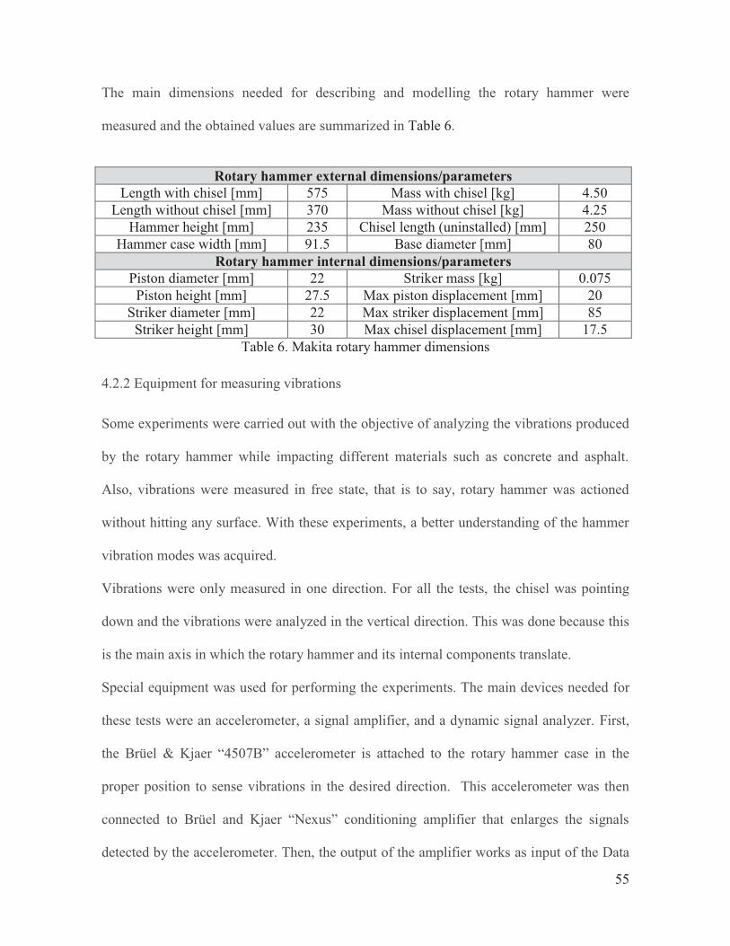
The main dimensions needed for describing and modelling the rotary hammer were
measured and the obtained values are summarized in Table 6.
Rotary hammer external dimensions/parameters
Length with chisel [mm] 575 Mass with chisel [kg] 4.50 Length without chisel [mm] 370 Mass without chisel [kg] 4.25
Hammer height [mm] 235 Chisel length (uninstalled) [mm] 250 Hammer case width [mm] 91.5 Base diameter [mm] 80
Rotary hammer internal dimensions/parameters Piston diameter [mm] 22 Striker mass [kg] 0.075 Piston height [mm] 27.5 Max piston displacement [mm] 20
Striker diameter [mm] 22 Max striker displacement [mm] 85 Striker height [mm] 30 Max chisel displacement [mm] 17.5
Table 6. Makita rotary hammer dimensions
4.2.2 Equipment for measuring vibrations
Some experiments were carried out with the objective of analyzing the vibrations produced
by the rotary hammer while impacting different materials such as concrete and asphalt.
Also, vibrations were measured in free state, that is to say, rotary hammer was actioned
without hitting any surface. With these experiments, a better understanding of the hammer
vibration modes was acquired.
Vibrations were only measured in one direction. For all the tests, the chisel was pointing
down and the vibrations were analyzed in the vertical direction. This was done because this
is the main axis in which the rotary hammer and its internal components translate.
Special equipment was used for performing the experiments. The main devices needed for
these tests were an accelerometer, a signal amplifier, and a dynamic signal analyzer. First,
the Brüel & Kjaer “4507B” accelerometer is attached to the rotary hammer case in the
proper position to sense vibrations in the desired direction. This accelerometer was then
connected to Brüel and Kjaer “Nexus” conditioning amplifier that enlarges the signals
detected by the accelerometer. Then, the output of the amplifier works as input of the Data
56
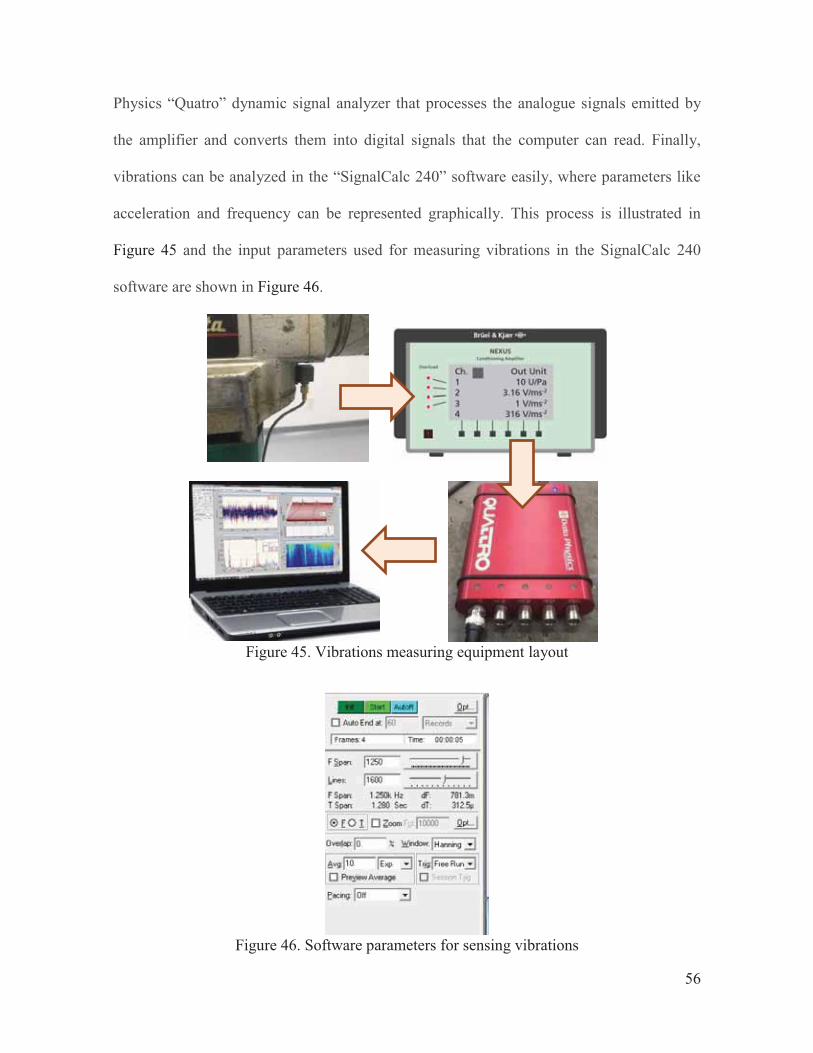
Physics “Quatro” dynamic signal analyzer that processes the analogue signals emitted by
the amplifier and converts them into digital signals that the computer can read. Finally,
vibrations can be analyzed in the “SignalCalc 240” software easily, where parameters like
acceleration and frequency can be represented graphically. This process is illustrated in
Figure 45 and the input parameters used for measuring vibrations in the SignalCalc 240
software are shown in Figure 46.
Figure 45. Vibrations measuring equipment layout
Figure 46. Software parameters for sensing vibrations

57
Three experiments were carried out in order to be able to understand and analyze the
vibrations produced by the impact tool chosen.
4.2.3 Makita rotary hammer experiments
� Experiment 1. Without impact
The first experiment was performed without contact with other surfaces. The rotary
hammer was actioned for a few seconds and the vibrations produced by the movement of
its internal components were registered. The obtained results are shown in Figure 47 and
Figure 48.
Figure 47. Rotary hammer vibrations without impacts
Figure 48. Frequencies of vibration (without impacts)
In the previous experiments, three main frequencies are identified.
� F1 = 72.66 Hz
� F2 = 145.3 Hz
� F3 = 315.6 Hz
120m 140m 160m-300m
-200m
-100m
0
100m
200m
300m
sec
Rea
l, V
X1
X1 X: 318.7m Y: -22.58m
0 200 400 600 800 1.0k-120
-100
-80
-60
-40
-20
0
Hz
dBM
ag, V
G1, 1 X: 315.6 Y: -28.40

58
It is evident that the first two frequencies are harmonic ones, as F2 is two times F1.
However, F3 represents a peak for another mode of vibration.
Next, two impact tests were done as it is shown in Figure 50. The first test was done against
an asphalt cylinder and the second one with a concrete sample (Rc=250 kg/cm2). Both test
samples were created in the universities pavements laboratory and are presented in Figure
49.
Figure 49. Test samples
Figure 50. Tests on asphalt (left) and concrete (right)
59
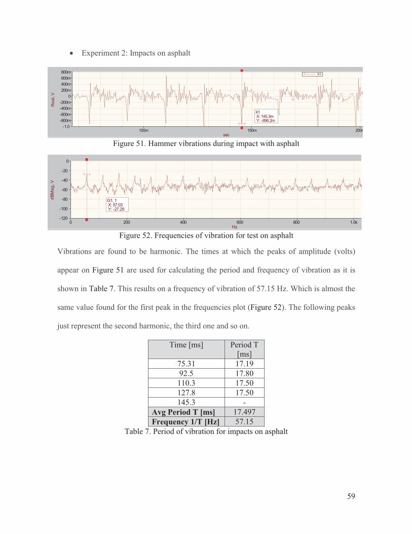
� Experiment 2: Impacts on asphalt
Figure 51. Hammer vibrations during impact with asphalt
Figure 52. Frequencies of vibration for test on asphalt
Vibrations are found to be harmonic. The times at which the peaks of amplitude (volts)
appear on Figure 51 are used for calculating the period and frequency of vibration as it is
shown in Table 7. This results on a frequency of vibration of 57.15 Hz. Which is almost the
same value found for the first peak in the frequencies plot (Figure 52). The following peaks
just represent the second harmonic, the third one and so on.
Time [ms] Period T [ms]
75.31 17.19 92.5 17.80 110.3 17.50 127.8 17.50 145.3 -
Avg Period T [ms] 17.497 Frequency 1/T [Hz] 57.15
Table 7. Period of vibration for impacts on asphalt
100m 150m 200m-1.0
-800m-600m-400m-200m
0200m400m600m800m
sec
Rea
l, V
X1
X1 X: 145.3m Y: -896.2m
0 200 400 600 800 1.0k-120
-100
-80
-60
-40
-20
0
Hz
dBM
ag, V
G1, 1 X: 57.03 Y: -27.29

60
� Experiment 3: Impacts on concrete
Figure 53. Hammer vibrations during impact with concrete
Figure 54. Frequencies of vibration for test on concrete
The results obtained in the experiments performed on concrete are very similar to the ones
obtained with asphalt. In both cases, vibrations reach amplitudes of more than one volt. The
frequency of the first harmonic is 57.8 Hz (Figure 54), almost the same one as in the
previous test.
However, acceleration of vibration cannot be obtained straight forward from the software,
further interpretation is required. For this purpose, a calibration exciter is needed to convert
the volts obtained as vibrations to acceleration in m/s2. The calibration exciter used is the
Type 4294 also from Brüel & Kjaer. This device is an electromagnetic exciter with an
internal built in piezoelectric accelerometer for servo regulation of amplitude. The exciter
can be seen in Figure 55.
100m 150m 200-1.0
-800m-600m-400m-200m
0200m400m600m800m
sec
Rea
l, V
X1
X1 X: 83.44m Y: -1.067
0 200 400 600 800 1.0k-120
-100
-80
-60
-40
-20
0
Hz
dBM
ag, V
G1, 1 X: 57.81 Y: -25.91

61
Figure 55. Brüel & Kjaer calibration exciter
The calibrator vibrates at a known frequency (f=159.15 Hz ± 0.02%) and an acceleration of
10 m/s2. With these values, the calibrator is turned on and vibrations are measured with the
same equipment used for the tests. Voltage and frequencies of vibration are obtained and
from this a constant is calculated to determine the acceleration and amplitude of vibration
of the values registered in the tests.
Figure 56. Vibrations produced by calibration exciter
Figure 57. Frequencies of vibration of calibration exciter
The results obtained in the calibration are: z, , and
With these values a conversion constant is calculated:

62
Then, with this constant, the maximum acceleration of vibrations for tests in asphalt and
concrete can be determined. Voltage obtained for both concrete and asphalt is very similar
so a common value is used.
The frequency of the first harmonic can be used to compute the amplitude of these peaks of
vibration in millimetres.
This value represents the magnitude in millimeters of the maximum peak of vibration as a
result of the superposition of all the frequencies involved in the production of the hammer
impacts.
Though, the amplitude of just the first mode of vibration can be determined with the
decibels and the frequency of the first harmonic.
Calibration Exciter Rotary hammer (Impacts on concrete
159 Hz 57.8 Hz
dB -34.2 -25.91
Table 8. Frequency of the 1st harmonic for exciter and hammer
Using equation (2.1) acceleration of the first harmonic can be found in the following way:
(4.1)
(4.2)
Expression (4.2) is subtracted from expression (4.1) and the next equation is obtained

63
It is important to mention that, for the development of these expressions, the vibrations of
the exciter are assumed to be harmonic, neglecting the secondary peaks found in the
frequency spectre shown in Figure 57.
The result of the calculation can be verified with the values for continuous vibration levels
for a rotary hammer presented in Table 1, were typical range varies from 5 to 24 m/s2.
The obtained frequencies can be applied in the mathematical models developed and the
possibility of damping the first modes of vibration can be determined. Also, a comparison
can be made between the amplitudes of vibration measured and the values obtained in the
models.
4.3 Modelling of rotary hammer – Kinetic model with algebraic equations
The rotary hammer working principle was modeled in two ways. A first model was
proposed based on rigid body kinetics theory. There are two main elements that constitute
this model, the piston and the striker. This model tries to imitate the motion of this tool.
The piston goes back and forth as part of a crank-rod mechanism with a sinusoidal motion.
While doing it, the piston hits the striker which translates towards the chisel. In this case,
the chisel is assumed to be static due to the minimum displacement it experiences and the
way the shockwaves travel through it. Figure 58 helps to visualize the proposed model.

64
Figure 58. Rotary hammer modelling
Where,
1, corresponds to the piston
2, corresponds to the striker
3, corresponds to the chisel (assumed as static)
x, is the position of the striker along horizontal axis
z, is the position of the piston
e, is the maximum displacement of the striker
The governing equations developed for describing the behavior of these elements are
presented as follows.
The motion of the piston is:
(4.3)
Where ω, is the angular velocity of the piston and is the amplitude of its movement.
The time for first impact (t1) - Piston vs Striker reads:
(4.4)
Where x0, is the position of the striker.
The velocity of piston after first impact (vz1) is:
(4.5)
1 2
3
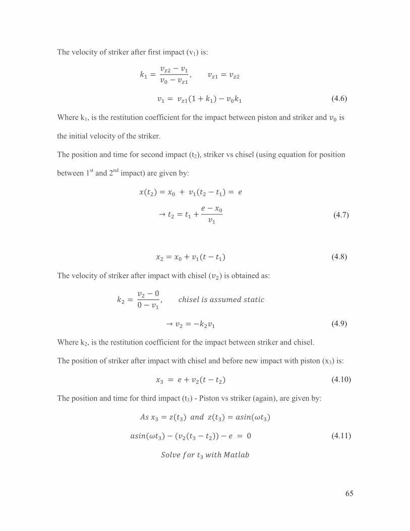
65
The velocity of striker after first impact (v1) is:
(4.6)
Where k1, is the restitution coefficient for the impact between piston and striker and is
the initial velocity of the striker.
The position and time for second impact (t2), striker vs chisel (using equation for position
between 1st and 2nd impact) are given by:
(4.7)
(4.8)
The velocity of striker after impact with chisel ( ) is obtained as:
(4.9)
Where k2, is the restitution coefficient for the impact between striker and chisel.
The position of striker after impact with chisel and before new impact with piston (x3) is:
(4.10)
The position and time for third impact (t3) - Piston vs striker (again), are given by:
(4.11)

66
Finally, the velocity of striker after impact with piston is:
(4.12)
In addition to these equations, a special case was found that needed further attention. This
case is illustrated in Figure 59 and it happens when the piston (z) is coming back and the
striker (x) is moving at higher velocity so they collide on their way back. Therefore, the
striker bounces back but with less energy. Hence, if the striker is moving too slow, the
piston could make a complete cycle and be able to hit the striker again.
Figure 59. Striker (x) colliding with returning piston (z)
This extra collision with the piston is the one considered in these equations.
As time for impact in this special case (tsp) is unknown, it has to be determined before
computing the velocity of the striker after this second impact, as follows:
(4.13)
The velocity of striker after being hit by piston twice is:
(4.14)
The average forces exerted on each impact are computed by using the equation of
Conservation of Linear Momentum.

67
(4.15)
Where, G1 and G2 are the linear momentum at time t1 and t2, respectively. Also, V1 and V0
stand for the velocity of the body before and after impact, m is the mass of the body and ∆t
represents the duration of the impact as a really short amount of time.
It is important to mention that the maximum force is two times bigger than the average
force.
Matlab program was developed with these equations with the objective of obtaining a
graphical representation of the behavior of the rotary hammer inner components.
4.3.1 Matlab application
Again, the equations shown in last section are programmed in Matlab with the purpose of
being able to play with the different parameters that define the system and observe, in a
graphic way, the obtained results. Matlab code is programmed in different sections.
Functions that describe the displacement and the velocity of the piston and the striker are
defined first. Subsequently, they are called inside a cyclic structure for computing the
parameters according to the number of impacts given by the simulation time defined.
Input parameters for this program are:
, striker initial position [mm] , initial velocity of striker [mm/s]
, striker maximum displacement [mm] , amplitude of piston’s movement [mm] , restitution coefficient for impact between piston-striker [-]

68
, restitution coefficient for impact between striker and chisel [-] , angular velocity of the piston [rad/s] , simulation time [s] , mass of the striker [kg]
, time delta of impact duration between piston and striker [s] , time delta of impact duration between striker and chisel [s]
The following parameters apply for the 3 cases that are going to be presented in this
section: x0 = 5 mm, v0 = 0 m/s, e = 85 mm, a=10 mm, tf = 3 s, m = 0.075 kg, dt1 = 0.003 s,
dt2 =0.002 s.
� Experiment 1: ω = 70 rad/s, k1 = 0.7, k2 = 0.8
Figure 60. Experiment 1 (kinetic model)
In the first chart of Figure 60, the black line represents the motion of the striker; whereas
the red sinusoidal curve represents the motion of the piston. Then, every time these lines
touch each other, it means the piston has just hit the striker.

69
The velocity of the striker shown in chart 2 has a step-shape because its travelling direction
changes suddenly after each impact. That is why the velocity is constant during fractions of
a second and at a certain point, the striker hits either the chisel or the piston, bouncing away
in the opposite direction to the one it had before the impact.
In the case of the third chart of Figure 60, the average force is plotted with dots instead of a
continuous curve. This happens because the force is only present at the instant at which the
striker impacts another component, and it becomes zero whenever the striker is travelling
towards the other body.
� Experiment 2: ω = 100 rad/s, k1 = 0.7, k2 = 0.8
Figure 61. Experiment 2 (kinetic model)

70
� Experiment 3: ω = 100 rad/s, k1 = 0.5, k2 = 0.6
Figure 62. Experiment 3 (kinetic model)
In these experiments the impact of the angular velocity of the piston and the restitution
coefficient on the model is reviewed. From first to second experiment, the rotational speed
of the piston increases from 70 rad/s to 100 rad/s. This increases the travel speed of the
striker, as well as the average force produced at each impact. That is to say, the striker hits
the chisel 8 times in 0.5 seconds with ω=100 rad/s, whereas for the speed of ω=70 rad/s the
striker only hits the chisel in 6 occasions. Therefore, an increase in the angular velocity of
the piston would mean an increase on the velocity at which the striker travels resulting in
higher impact forces.
In the third case, the coefficients of restitution k1 and k2 are both reduced in 0.2 [-]. This
action means that the striker loses more energy on each impact than in the previous
experiments. Under these parameters, the striker only hits the chisel 4 times during the first
0.5 seconds. Additionally, there is a point (t=0.84 s) where the striker collides with the

71
piston on its way back. Therefore, the striker loses more energy than the usual and travels
back to the chisel at a very low speed causing the phenomenon observed in
Figure 62 (no striker-chisel collision for a long time) between the 0.84 s and the 2.53 s.
4.4 Modelling of rotary hammer – Dynamic model with differential equations
As it was already seen, the mathematical model from section 4.3 is based on algebraic
equations and served as a preliminary model for the system. Nevertheless, in order to
combine the model of a rotary hammer with the one of the Dynamic Eliminator of
Vibrations, both systems need to be based on the same type of equations, in this case,
differential equations.
For that reason, Newton’s Second Law is applied for the analysis of the rotary hammer
system. The first challenge encountered was to model the contacts piston-striker and
striker-chisel. In the real rotary hammer system, the piston and the striker are never in
contact. That is to say, the striker moves as a reaction of the air compression that piston
exerts on it. On the other hand, the striker actually hits the chisel, but they are in contact for
fractions of a second. Therefore, modelling of the link between these bodies was not
straight forward.
In order to be able to develop differential equations using Newton’s Second Law, both
interactions between the bodies were modelled as springs with two special characteristics.
The first characteristic is a really high stiffness for the springs. This idea is based on the
principle that a very stiff spring could represent an impact with a solid surface. The second
characteristic refers to the action of making the spring forces zero whenever two bodies are
not in contact. Additionally, damping is added between each body to take into
consideration the energy loss after each impact. This approach is illustrated in Figure 63.
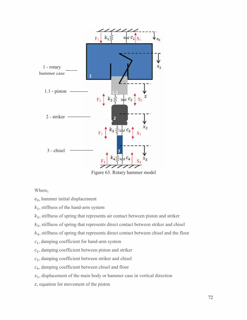
72
Figure 63. Rotary hammer model
Where,
, hammer initial displacement
, stiffness of the hand-arm system
, stiffness of spring that represents air contact between piston and striker
, stiffness of spring that represents direct contact between striker and chisel
, stiffness of spring that represents direct contact between chisel and the floor
, damping coefficient for hand-arm system
, damping coefficient between piston and striker
, damping coefficient between striker and chisel
, damping coefficient between chisel and floor
, displacement of the main body or hammer case in vertical direction
, equation for movement of the piston
1 - rotary hammer case
1.1 - piston
2 - striker
3 - chisel
F4
F2 S2
F3 S3
S4
S1 F1

73
, displacement of the striker in vertical direction
, displacement of the chisel in vertical direction
, angular velocity of the piston crankshaft mechanism
The forces interacting in the system are defined in this way:
The governing equations for this system are obtained following Newton’s Second Law:
(4.16)
(4.17)
(4.18)
Just using springs to represent the impact between components would mean that they are
always in contact. For that reason, an extra condition is added to the formulation of
, the forces that represent the impacts between piston-striker, striker-chisel and
chisel-surface, respectively. This formulation specifies that if the resultant force of these
springs is negative, the force will be automatically equal to 0. This only happens when
is smaller than 0.
Springs
Dampers

74
It is important to mention that is considered as the displacement of the upper body
minus the one of the lower body (see Figure 63), i.e. for the contact striker-chisel,
. Hence, if , means that and that the striker and chisel are being
displaced away from each other, avoiding any interaction.
4.4.1 Matlab application
This system is also modelled in Matlab to observe the behaviour of all the internal elements
of the hammer, as well as the produced forces.
The independent degrees of freedom identified in Figure 63 are listed below for
constituting the differential equations system for Matlab solution with function ode45.
Furthermore, the system of equations is defined as:
Input parameters are given to the system and the results are plotted as in previous
applications.
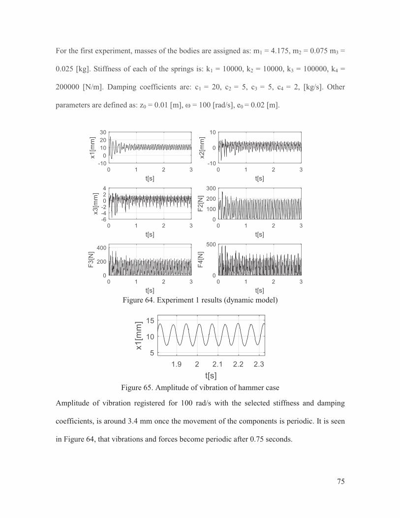
75
For the first experiment, masses of the bodies are assigned as: m1 = 4.175, m2 = 0.075 m3 =
0.025 [kg]. Stiffness of each of the springs is: k1 = 10000, k2 = 10000, k3 = 100000, k4 =
200000 [N/m]. Damping coefficients are: c1 = 20, c2 = 5, c3 = 5, c4 = 2, [kg/s]. Other
parameters are defined as: z0 = 0.01 [m], ω = 100 [rad/s], e0 = 0.02 [m].
Figure 64. Experiment 1 results (dynamic model)
Figure 65. Amplitude of vibration of hammer case
Amplitude of vibration registered for 100 rad/s with the selected stiffness and damping
coefficients, is around 3.4 mm once the movement of the components is periodic. It is seen
in Figure 64, that vibrations and forces become periodic after 0.75 seconds.
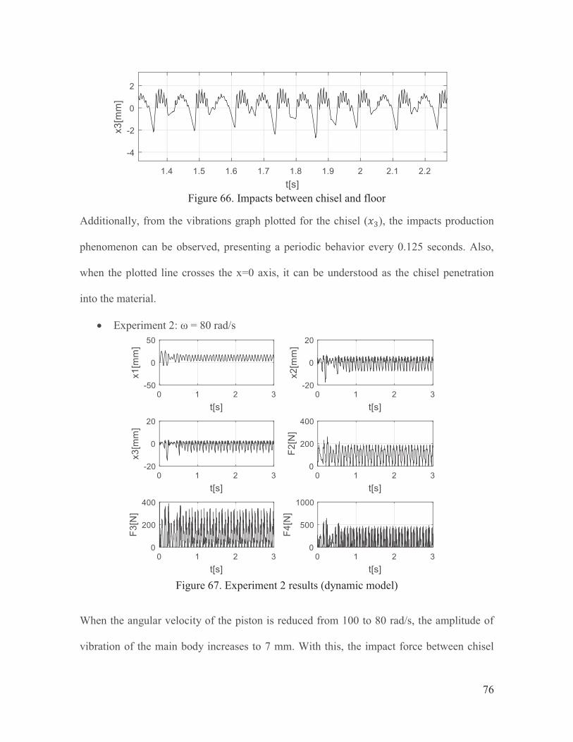
76
Figure 66. Impacts between chisel and floor
Additionally, from the vibrations graph plotted for the chisel ( ), the impacts production
phenomenon can be observed, presenting a periodic behavior every 0.125 seconds. Also,
when the plotted line crosses the x=0 axis, it can be understood as the chisel penetration
into the material.
� Experiment 2: ω = 80 rad/s
Figure 67. Experiment 2 results (dynamic model)
When the angular velocity of the piston is reduced from 100 to 80 rad/s, the amplitude of
vibration of the main body increases to 7 mm. With this, the impact force between chisel
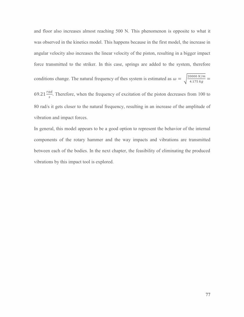
77
and floor also increases almost reaching 500 N. This phenomenon is opposite to what it
was observed in the kinetics model. This happens because in the first model, the increase in
angular velocity also increases the linear velocity of the piston, resulting in a bigger impact
force transmitted to the striker. In this case, springs are added to the system, therefore
conditions change. The natural frequency of thes system is estimated as
Therefore, when the frequency of excitation of the piston decreases from 100 to
80 rad/s it gets closer to the natural frequency, resulting in an increase of the amplitude of
vibration and impact forces.
In general, this model appears to be a good option to represent the behavior of the internal
components of the rotary hammer and the way impacts and vibrations are transmitted
between each of the bodies. In the next chapter, the feasibility of eliminating the produced
vibrations by this impact tool is explored.
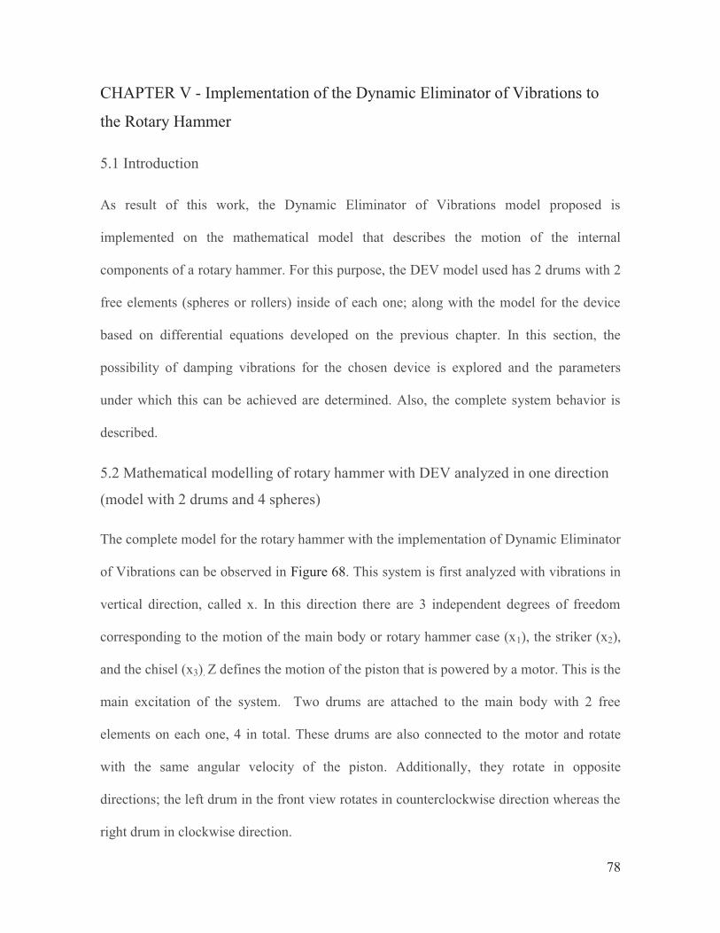
78
CHAPTER V - Implementation of the Dynamic Eliminator of Vibrations to
the Rotary Hammer
5.1 Introduction
As result of this work, the Dynamic Eliminator of Vibrations model proposed is
implemented on the mathematical model that describes the motion of the internal
components of a rotary hammer. For this purpose, the DEV model used has 2 drums with 2
free elements (spheres or rollers) inside of each one; along with the model for the device
based on differential equations developed on the previous chapter. In this section, the
possibility of damping vibrations for the chosen device is explored and the parameters
under which this can be achieved are determined. Also, the complete system behavior is
described.
5.2 Mathematical modelling of rotary hammer with DEV analyzed in one direction
(model with 2 drums and 4 spheres)
The complete model for the rotary hammer with the implementation of Dynamic Eliminator
of Vibrations can be observed in Figure 68. This system is first analyzed with vibrations in
vertical direction, called x. In this direction there are 3 independent degrees of freedom
corresponding to the motion of the main body or rotary hammer case (x1), the striker (x2),
and the chisel (x3). Z defines the motion of the piston that is powered by a motor. This is the
main excitation of the system. Two drums are attached to the main body with 2 free
elements on each one, 4 in total. These drums are also connected to the motor and rotate
with the same angular velocity of the piston. Additionally, they rotate in opposite
directions; the left drum in the front view rotates in counterclockwise direction whereas the
right drum in clockwise direction.
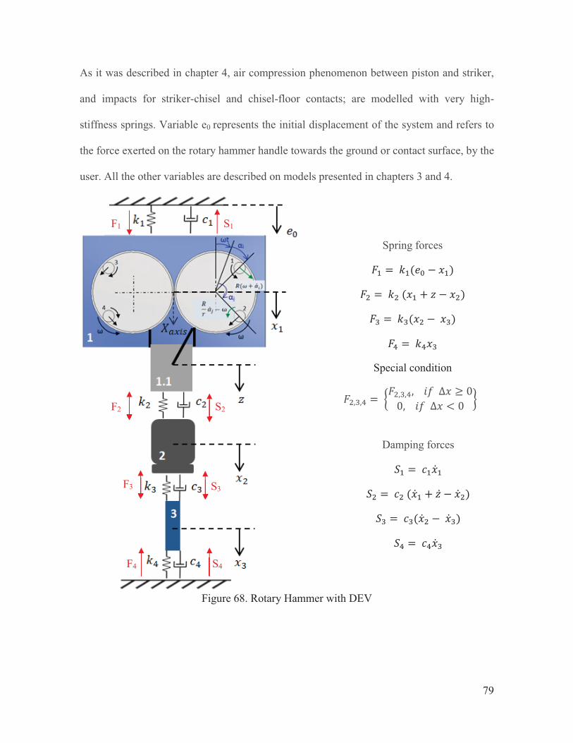
79
As it was described in chapter 4, air compression phenomenon between piston and striker,
and impacts for striker-chisel and chisel-floor contacts; are modelled with very high-
stiffness springs. Variable e0 represents the initial displacement of the system and refers to
the force exerted on the rotary hammer handle towards the ground or contact surface, by the
user. All the other variables are described on models presented in chapters 3 and 4.
Figure 68. Rotary Hammer with DEV
Spring forces
Special condition
Damping forces
F4
F2 S2
F3 S3
S4
S1 F1

80
Governing equations for this system obtained with Lagrange equations for the DEV
section, equations (3.8), (3.9) and Newton’s 2nd law equations (4.16)-(4.18) for the rotary
hammer components are brought up together and presented here:
(5.1)
(5.2)
(5.3)
(5.4)
Where,
And, is the mass of the free elements
The sign in the equations of and related to the vertical displacement of the free
elements changes because the positive values are considered downwards for the
independent coordinates x1, x2, x3.
Again, is substituted by variable and term is neglected due to its
small magnitude and unimportant affection to the final result.
(5.5)
(5.6)
(5.7)

81
(5.8)
This system of equations is again solved with the help of Matlab. Thus, results and basis of
Matlab code can be seen in the next section.
5.2.1 Matlab application
First, the independent degrees of freedom are listed as follows for a DEV model of 4 free
elements, two inside each drum:
Therefore, the system of equations is defined as:

82
Finally, the term in the expressions of is substituted by
for its solution. Full Matlab code can be reviewed in appendix section of this document.
The masses assigned to the model are the ones obtained from the Makita rotary hammer
presented in chapter 3. The stiffness of the springs and the damping coefficients elected in
previous section are suitable for this model.
The mass of hammer case including piston (m1) is 4.175 kg. The mass of the striker (m2) is
0.075 kg, whereas the mass of the chisel (m3) is 0.25 kg. The angular velocity of the piston
(excitation frequency) is 100 rad/s ≈ 950 rpm. The damping coefficients between each
impact are c1 = 20 kg/s; c2 = 5 kg/s; c3 = 5 kg/s; c4 = 2 kg/s; cR = 2 rad/s. The stiffness of the
hand-arm system is k1=10000 N/m. The stiffness of the springs that represent impacts are
k2=10000 N/m; k3=100000 N/m; k4=200000 N/m. The radius of the drums is R=0.05 m.
The amplitude of the piston translation is z0 = 0.01 [m], and the handle initial displacement
is e0 = 0.02 [m].

83
Due to the complexity of this new system, the mass of the spheres is determined from trial
and error, by running the code several times until a proper value is found. A mass of 0.05
kg allows the system to absorb the produced vibrations of .
Then, with the density of the steel the radius of the spheres is computed.
Consequently, the system is solved with these parameters and the results are shown in
Figure 69. For this case, initial positions of the spheres were = 2.8 rad; = 3.2
rad.
Figure 69. Vibrations of the rotary hammer with 4-ball DEV

84
Figure 70. Forces in rotary hammer with 4-ball DEV
Final position of free elements Left drum Right drum
α3 2.6703 rad 153°
α1 2.6703 rad 153°
α4 3.7026 rad 212.14°
α2 3.7026 rad 212.14°
Table 9. Equilibrium position of free elements in DEV application to rotary hammer
Figure 71. Equilibrium position diagram for DEV

85
Vibrations are reduced from 5 mm of initial amplitude to 0.07 mm in just 4 seconds. After
6 seconds vibrations practically disappear.
Figure 72. Vibrations absorption
Vibrations of the chisel as well as the exerted forces on the ground behave in the following
way. Amplification is done to Figure 69 and Figure 70 for better appreciation of vibrations.
Figure 73. Vibrations of the chisel
A second experiment is run to explore the effect of the viscous damping (produced by the
fluid inside the drums) on the movement of the main body or hammer case.
If the viscous damping for the spheres is increased by 4 times (cR = 8 rad/s) vibrations are
fully damped in approximately 3.5 seconds. Also, it is easier for the free elements to find
and stay in the equilibrium position because the residual forces that try to push them away
from this position are not enough to overcome the viscous damping force. This can be seen
in Figure 74.

86
Figure 74. Influence of increase in viscous damping coefficient.
However, if the viscous damping coefficient is now reduced 4 times (cR = 0.5 rad/s) is not
possible of the DEV to eliminate the vibrations of the main body.
Figure 75. Influence of reduction in viscous damping coefficient.
As it can be observed in Figure 75, where is plotted against , the free elements inside
the drum are not able to find a stable position that can counteract the forces exerted on the
main body due to the excitation of the system. In this case other parameters such as the
mass of the spheres would need to be adjusted to explore the possibility of damping
vibrations.
It is also important to mention that Forces F2, F3 and F4 are not really affected by the
increase or reduction of the viscous damping coefficient, their magnitude remains almost

87
the same. Full results of these experiments can be seen in the appendix section of this
document.
5.3 Mathematical modelling of rotary hammer with DEV analyzed in two directions
(model with 2 drums and 4 spheres)
The next stage of this work is to analyze the system developed in the previous section but
in two directions of the coordinate system. Now, translation is not only considered in the
vertical direction (x axis) but also in the horizontal one (y axis) for the main body. Bodies
3, 4 that represent the striker and chisel in the system are only analyzed in the x axis.
Moreover, a spring is added to the rotary hammer that actuates in y-direction and represents
the stiffness of the user’s hand-arm system and the force exerted by actuating the tool.
Besides, a damper is also added representing natural conditions of the vibration attenuating
process.
It is important to mention that this damping coefficient added to the system of equations is
needed to show the vibrations amplitude reduction in both directions. This happens because
a DEV is only capable of damping excited vibrations but it cannot absorb the vibrations
produced by the natural frequencies of a system. In this case, the excitation is only provided
in the vertical direction, therefore DEV does not really work for the horizontal direction.
The system’s equations are very similar to those presented in section 5.2.

88
Figure 76. Rotary Hammer with DEV (XY analysis)
The special condition for the springs that represent an impact is also added as:
Lagrange equations method is applied for each of the independent coordinates. The
development of the equations for is already presented in section 5.2 for
equations (5.5)-(5.7). For the new independent degree of freedom, associated with
vibrations along the horizontal axis, named as Y, the equation is obtained as follows.
Spring forces
Damper forces
F4
F2 S2
F3 S3
S4
S1 F1

89
Kinetic and potential energy are expressed as defined by the Lagrange equation as:
Kinetic energy:
(5.9)
Potential energy due to springs:
(5.10)
Non-conservative forces are obtained from virtual work equation (
). These forces are caused by damper action:
(5.11)
(5.12)
for
for
for
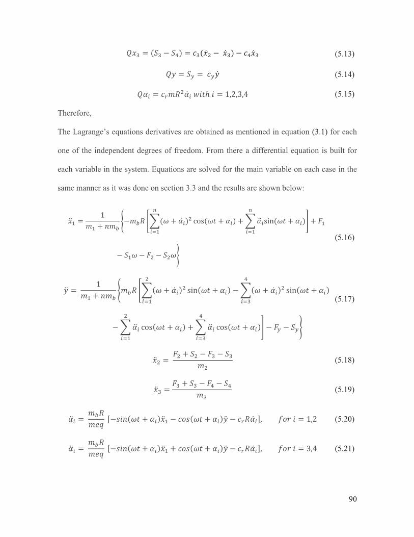
90
Therefore,
The Lagrange’s equations derivatives are obtained as mentioned in equation (3.1) for each
one of the independent degrees of freedom. From there a differential equation is built for
each variable in the system. Equations are solved for the main variable on each case in the
same manner as it was done on section 3.3 and the results are shown below:
(5.13)
(5.14)
(5.15)
(5.16)
(5.17)
(5.18)
(5.19)
(5.20)
(5.21)

91
In the is neglected due to the small impact it has on the equation,
as well as the terms for the equation,
where the value of this part of the equation is very small compared to the other terms.
Then, these equations are solved for the main independent variable on each case and ωt is
again substituted by time τ.
(5.22)
(5.23)
(5.24)
(5.25)
(5.26)
(5.27)
5.3.2 Matlab application
Due to the complexity of the system, the second degree differential equations are converted
into first degree equations for its solution in Matlab. Similar to what was done for the other
models, the system is solved with function ode45. The complete code is showed in
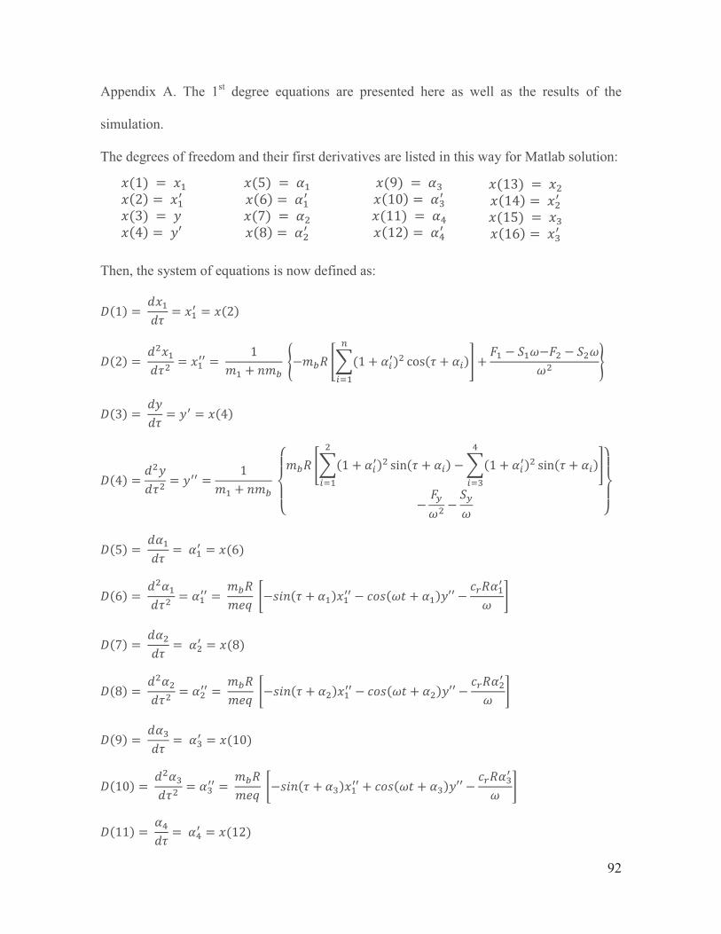
92
Appendix A. The 1st degree equations are presented here as well as the results of the
simulation.
The degrees of freedom and their first derivatives are listed in this way for Matlab solution: Then, the system of equations is now defined as:
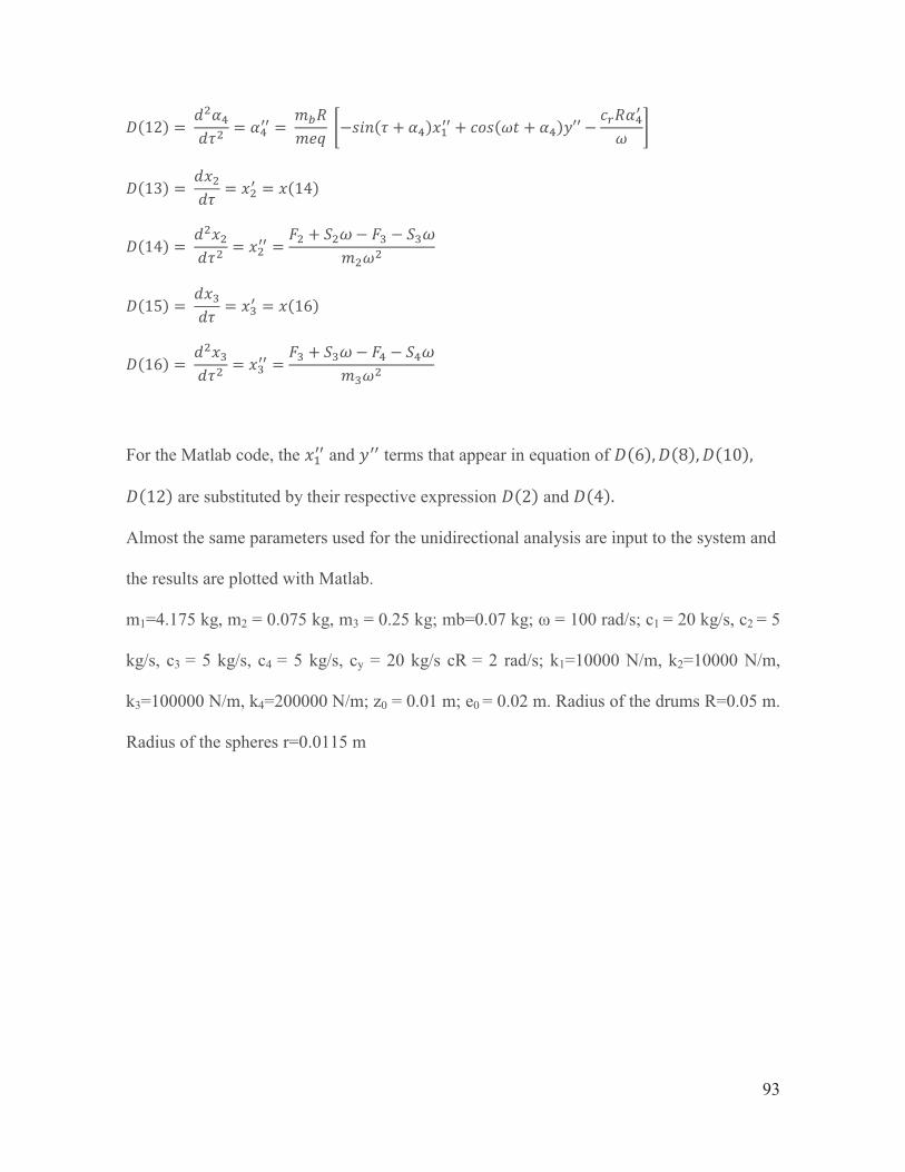
93
For the Matlab code, the and terms that appear in equation of
are substituted by their respective expression and
Almost the same parameters used for the unidirectional analysis are input to the system and
the results are plotted with Matlab.
m1=4.175 kg, m2 = 0.075 kg, m3 = 0.25 kg; mb=0.07 kg; ω = 100 rad/s; c1 = 20 kg/s, c2 = 5
kg/s, c3 = 5 kg/s, c4 = 5 kg/s, cy = 20 kg/s cR = 2 rad/s; k1=10000 N/m, k2=10000 N/m,
k3=100000 N/m, k4=200000 N/m; z0 = 0.01 m; e0 = 0.02 m. Radius of the drums R=0.05 m.
Radius of the spheres r=0.0115 m
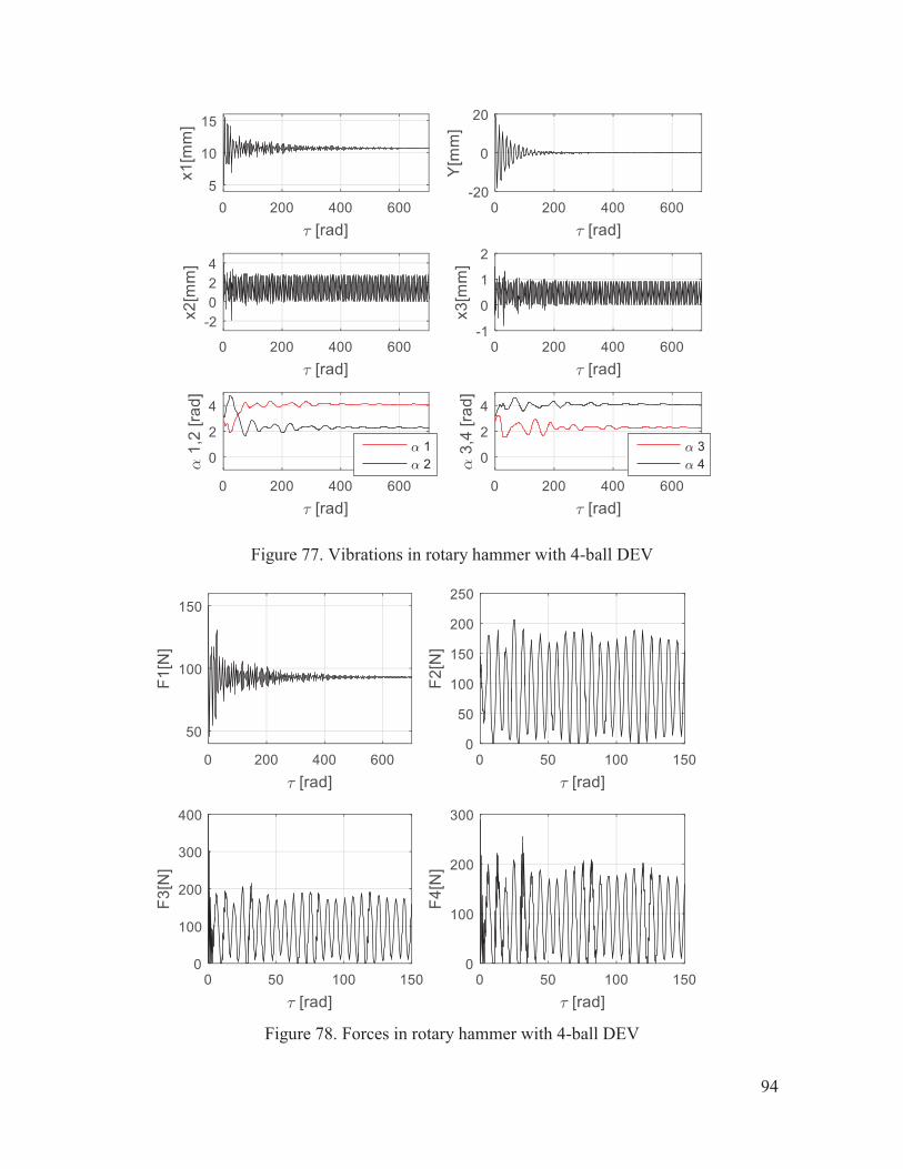
94
Figure 77. Vibrations in rotary hammer with 4-ball DEV
Figure 78. Forces in rotary hammer with 4-ball DEV
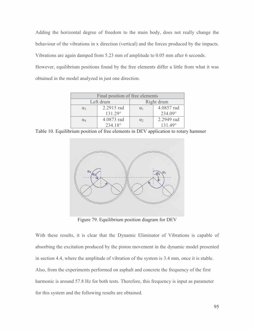
95
Adding the horizontal degree of freedom to the main body, does not really change the
behaviour of the vibrations in x direction (vertical) and the forces produced by the impacts.
Vibrations are again damped from 5.23 mm of amplitude to 0.05 mm after 6 seconds.
However, equilibrium positions found by the free elements differ a little from what it was
obtained in the model analyzed in just one direction.
Final position of free elements
Left drum Right drum α3 2.2915 rad
131.29° α1 4.0857 rad
234.09° α4 4.0873 rad
234.18° α2 2.2949 rad
131.49° Table 10. Equilibrium position of free elements in DEV application to rotary hammer
Figure 79. Equilibrium position diagram for DEV
With these results, it is clear that the Dynamic Eliminator of Vibrations is capable of
absorbing the excitation produced by the piston movement in the dynamic model presented
in section 4.4, where the amplitude of vibration of the system is 3.4 mm, once it is stable.
Also, from the experiments performed on asphalt and concrete the frequency of the first
harmonic is around 57.8 Hz for both tests. Therefore, this frequency is input as parameter
for this system and the following results are obtained.

96
As the excitation frequency changes from 100 rad/s to 365 rad/s, a new mass needs to be
determined in order to counteract the excitation force. As a starting point for the iterations
the initial mass computed is:
After some simulations optimal mass determined is: 0.007 kg. If free elements are to be
steel balls, they would have a radius of 6 mm.
Figure 80. Vibrations results with f=57.8 Hz

97
Figure 81. Forces of the system with f=57.8 Hz
Final position of free elements Left drum Right drum
α3 2.3774 rad 136.2°
α1 2.4136 rad 138.3°
α4 4.5328 rad 259.7°
α2 4.4816 rad 256.8°
Figure 82. Equilibrium positions when f=57.8 Hz
As the frequency of rotation of the drums is higher, the centrifugal force of the elements
also increases. Therefore, less mass is needed to counteract the excitation force. Then, this
space in this model can be optimized through several iterations of mass and radius of the
spheres, resulting in smaller drums. The next iteration results in a mass of 20 grams (0.02
kg) and a sphere radius of 4 mm (for steel). This allows having a drum radius of 20 mm
instead of 50 mm. This system results are presented in the next figure. It is important to
mention that as ω=365 rad/s. Time of simulation ωt=1000 rad is equal to 2.74 seconds.

98
Figure 83. System's optimization results
In these two cases, vibrations seem to be damped faster; however, it is harder for the free
elements to remain in the equilibrium position due to the high rotation velocities.
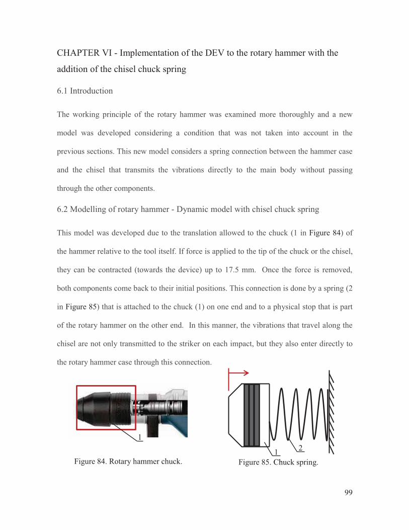
99
CHAPTER VI - Implementation of the DEV to the rotary hammer with the
addition of the chisel chuck spring
6.1 Introduction
The working principle of the rotary hammer was examined more thoroughly and a new
model was developed considering a condition that was not taken into account in the
previous sections. This new model considers a spring connection between the hammer case
and the chisel that transmits the vibrations directly to the main body without passing
through the other components.
6.2 Modelling of rotary hammer - Dynamic model with chisel chuck spring
This model was developed due to the translation allowed to the chuck (1 in Figure 84) of
the hammer relative to the tool itself. If force is applied to the tip of the chuck or the chisel,
they can be contracted (towards the device) up to 17.5 mm. Once the force is removed,
both components come back to their initial positions. This connection is done by a spring (2
in Figure 85) that is attached to the chuck (1) on one end and to a physical stop that is part
of the rotary hammer on the other end. In this manner, the vibrations that travel along the
chisel are not only transmitted to the striker on each impact, but they also enter directly to
the rotary hammer case through this connection.
Figure 84. Rotary hammer chuck.
Figure 85. Chuck spring.
1
Chu1 2

100
Thus, this connection is added to the model presented in Figure 63 (section 4.4) and the
result is shown in Figure 86, where represents the chuck spring. All the variables used
for the model presented in section 5.3 are applied in the same manner. The expression for
the force of the chuck spring F5 is defined in two parts. The first part considers the normal
operating condition of the spring; whereas the second part considers a substantial increase
in the stiffness of the spring referring to the moment when the spring goes to “solid state”
(coils are in contact).
Figure 86. Rotary hammer with chuck spring
F4
F2 S2
F3 S3
S4
F1 S1
1 - rotary hammer case
1.1 - piston
2 - striker
3 - chisel

101
The forces that are acting over the rotary hammer are produced by the springs and dampers
present in the system. These forces are defined as:
The governing equations of the system are:
(6.1)
(6.2)
(6.3)
The system of equations is solved using Matlab and the results can be seen in section 6.2.1
of this document.
6.2.1 Matlab application
Furthermore, the system of equations is defined as:
Springs
Special conditions:
Dampers

102
The system is solved with Matlab and the obtained results are shown as follows.
Figure 87. Rotary hammer vibrations (model with chuck spring)
The first peaks of vibration of the rotary hammer in Figure 87 vary around 12.5 mm of
amplitude, however, once free vibrations are damped, vibrations of the system reach a
steady state were the amplitude of vibrations produced by the external excitation is of 3.7

103
mm. The plot of shows several impacts with small amplitudes during one second, which
represents the penetration of the chisel into the impacted surface.
Figure 88. Rotary hammer forces
In the plot for seen in Figure 88, there are 3 peaks that reach up to 140 N, whereas, after
0.5 seconds, the force shows a periodic value of 25 N. This phenomenon happens in the
beginning when the chisel chuck spring is taken to solid state, which increases the stiffness
and the reaction force of the spring.
For the input parameters given, the chisel hits the ground with a force of 260 N ( once
vibrations have reached a steady state.
This model shows a more approximate approach to the real hammer behaviour and the
complexity of impacts production.

104
6.3 Mathematical modelling of rotary hammer with chisel spring connection and
DEV implementation (2 directions, 2 drums, 4 spheres)
The Dynamic Eliminator of Vibrations is implemented to the new rotary hammer model, to
determine the possibility of damping the vibrations produced by the new rotary hammer
model proposed.
Figure 89. Rotary hammer with DEV and chuck spring
The governing equations for the system presented in Figure 89 are very similar to what it
was developed on equations (5.22) - (5.27). The new only affects the equations for the
main body and for the chisel .
F4
F2 S2
F3 S3
S4
F1 S1
F5
Spring force
For
For
Special condition
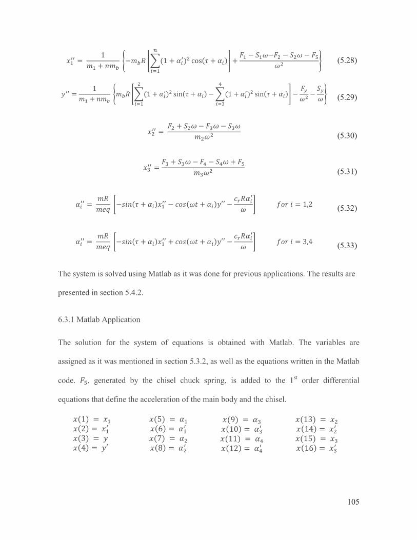
105
(5.28)
(5.29)
(5.30)
(5.31)
(5.32)
(5.33)
The system is solved using Matlab as it was done for previous applications. The results are
presented in section 5.4.2.
6.3.1 Matlab Application
The solution for the system of equations is obtained with Matlab. The variables are
assigned as it was mentioned in section 5.3.2, as well as the equations written in the Matlab
code. , generated by the chisel chuck spring, is added to the 1st order differential
equations that define the acceleration of the main body and the chisel.

106
Equations for the main body:
Equations for the chisel:
The rest of the equations are identical to the ones presented in section 5.3.2. Full Matlab
code is included in Appendix A.
The system is solved with the following input parameters.
n=8 DOF, m1 = 4.175 kg, m2 = 0.075 kg, m3 = 0.25 kg; ω=100 rad/s; c1 = 20 kg/s, c2 = 5
kg/s, c3 = 5 kg/s, c4 = 2 kg/s, cR = 5 rad/s; k1=10000 N/m, k2=10000 N/m, k3=100000 N/m,
k4=200000 N/m; k51 = 2000 N/m; k52 = 100 Nm; z0 = 0.01 m; e = 0.02 m; R=0.05 m; mb=
0.1 kg.
The radius of the spheres is computed with the proposed mass and the density of the steel.
The vibrations produced by the rotary hammer with this configuration and the
implementation of a 4-ball DEV are presented in Figure 90. Moreover, the forces produced
on each impact are plotted in Figure 91.
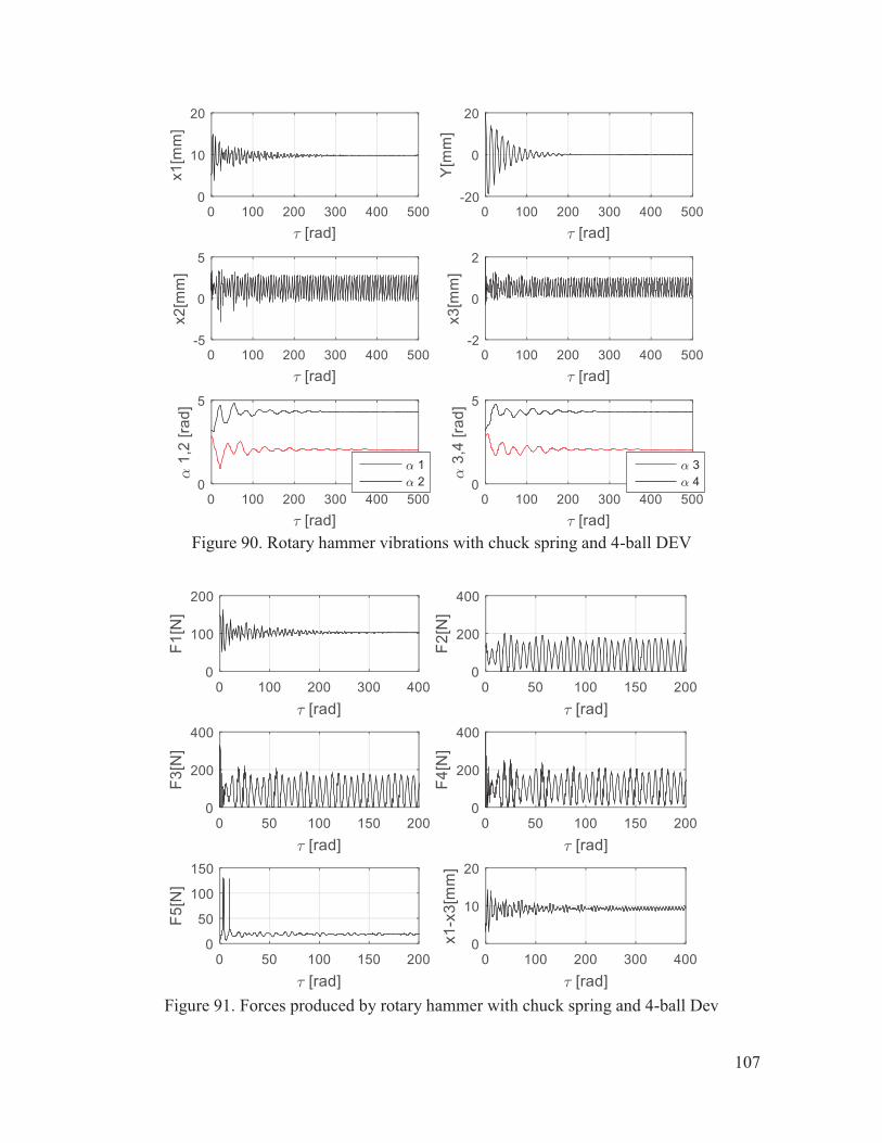
107
Figure 90. Rotary hammer vibrations with chuck spring and 4-ball DEV
Figure 91. Forces produced by rotary hammer with chuck spring and 4-ball Dev
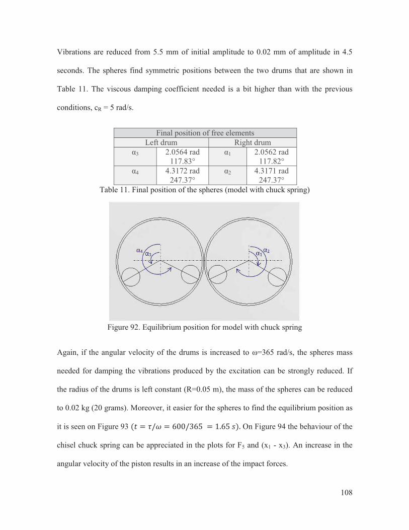
108
Vibrations are reduced from 5.5 mm of initial amplitude to 0.02 mm of amplitude in 4.5
seconds. The spheres find symmetric positions between the two drums that are shown in
Table 11. The viscous damping coefficient needed is a bit higher than with the previous
conditions, cR = 5 rad/s.
Final position of free elements Left drum Right drum
α3 2.0564 rad 117.83°
α1 2.0562 rad 117.82°
α4 4.3172 rad 247.37°
α2 4.3171 rad 247.37°
Table 11. Final position of the spheres (model with chuck spring)
Figure 92. Equilibrium position for model with chuck spring
Again, if the angular velocity of the drums is increased to ω=365 rad/s, the spheres mass
needed for damping the vibrations produced by the excitation can be strongly reduced. If
the radius of the drums is left constant (R=0.05 m), the mass of the spheres can be reduced
to 0.02 kg (20 grams). Moreover, it easier for the spheres to find the equilibrium position as
it is seen on Figure 93 On Figure 94 the behaviour of the
chisel chuck spring can be appreciated in the plots for F5 and (x1 - x3). An increase in the
angular velocity of the piston results in an increase of the impact forces.
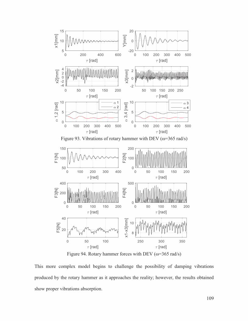
109
Figure 93. Vibrations of rotary hammer with DEV (ω=365 rad/s)
Figure 94. Rotary hammer forces with DEV (ω=365 rad/s)
This more complex model begins to challenge the possibility of damping vibrations
produced by the rotary hammer as it approaches the reality; however, the results obtained
show proper vibrations absorption.

110
CHAPTER VII - Conclusions
7.1 Conclusions
Vibrations are undesirable for most of mechanical systems and for the human body due to
the adverse effects they could provoke. Particularly, the long term use of impact tools could
lead to suffer disorders like the White Finger syndrome and the Dupuytren contracture.
Therefore, new ideas and technologies have been designed with the objective of damping
vibrations.
In this work, a rotary hammer working principle was mathematically modelled starting
from a simple approach and then developing a more complex dynamic system based on
Lagrange equations. This model shows amplitudes in the same order of magnitude
compared to the values obtained in the experiments performed on asphalt and concrete.
Then, the Dynamic Eliminator of Vibrations model proposed was implemented to the
rotary hammer and simulations were run. Even though detailed analysis was performed for
a system with 2 spheres per drum, it is possible to have more free elements.
Simulation results show that vibrations produced by a rotary hammer can be damped for
different parameters and conditions (ω tested from 80 rad/s to 365 rad/s) due to the
presence of the inertial force. This is only possible, with the proper update on sphere mass
and radius of the drums. It is important to mention that at higher angular velocities of the
drums; less mass is needed for system balance due to the increase in centrifugal force,
which allows space and mass optimization processes. Also, the increase in angular velocity
also shortens the response time of the free elements to find their equilibrium position.
111
The coefficient of viscous damping of the free elements also plays an important role in the
balancing process, because with the increase in this coefficient it is easier for the free
elements to stay in place, due to the produced forces.
The size of the device, according to the radius of the drums and the free elements, is
suitable for different applications depending on the excitation frequency of the system.
The Dynamic Eliminator of Vibrations was found to work properly only with excitation
frequencies that are above the natural frequency of the system. This vibration absorber can
be applied for the first harmonic of the system, which represents the mode of vibration with
the highest amplitude. However if two frequencies are to be damped, 2 sets of drums need
to be added to the system, each one rotating at one of the frequencies.
In general, this work served as application of all the knowledge acquired in the dynamics
and vibrations courses, along with programming abilities in Matlab. The proposed
objectives were accomplished leaving new ideas for future work.
7.2 Future work
Further development can be done in this project to validate the obtained results
mathematically with different methods, such as computer simulation of the modes of
vibration and the behaviour of the free elements. Moreover, Ideal Gas Law can be included
to the system’s modelling for describing the interaction between piston and striker.
Also, some other Matlab codes should be developed to investigate if a difference in
excitation frequency and rotational speed of the drum is allowed and until which ratio of
frequencies vibrations can still be damped.

112
Prototypes should be built and tested to analyze the behaviour of the system in real life. The
results of the tests should be compared with those obtained in Matlab and the simulations.
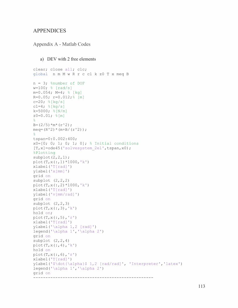
113
APPENDICES
Appendix A - Matlab Codes
a) DEV with 2 free elements
clear; close all; clc; global n m M w R r c c1 k z0 T x meq B n = 3; %number of DOF w=100; % [rad/s] m=0.054; M=4; % [kg] R=0.05; r=0.012;% [m] c=20; %[kg/s] c1=4; %[kg/s] k=5000; %[N/m] z0=0.01; %[m] % B=(2/5)*m*(r^2); meq=(R^2)*(m+B/(r^2)); % tspan=0:0.002:400; x0=[0; 0; 1; 0; 1; 0]; % Initial conditions [T,x]=ode45('solvesystem_2el',tspan,x0); %Plotting subplot(2,2,1); plot(T,x(:,1)*1000,'k') xlabel('T[rad]') ylabel('x[mm]') grid on subplot (2,2,2) plot(T,x(:,2)*1000,'k') xlabel('T[rad]') ylabel('v[mm/rad]') grid on subplot (2,2,3) plot(T,x(:,3),'k') hold on; plot(T,x(:,5),'r') xlabel('T[rad]') ylabel('\alpha 1,2 [rad]') legend('\alpha 1','\alpha 2') grid on subplot (2,2,4) plot(T,x(:,4),'k') hold on plot(T,x(:,6),'r') xlabel('T[rad]') ylabel('$\dot{\alpha}$ 1,2 [rad/rad]', 'Interpreter','latex') legend('\alpha 1','\alpha 2') grid on -------------------------------------------------
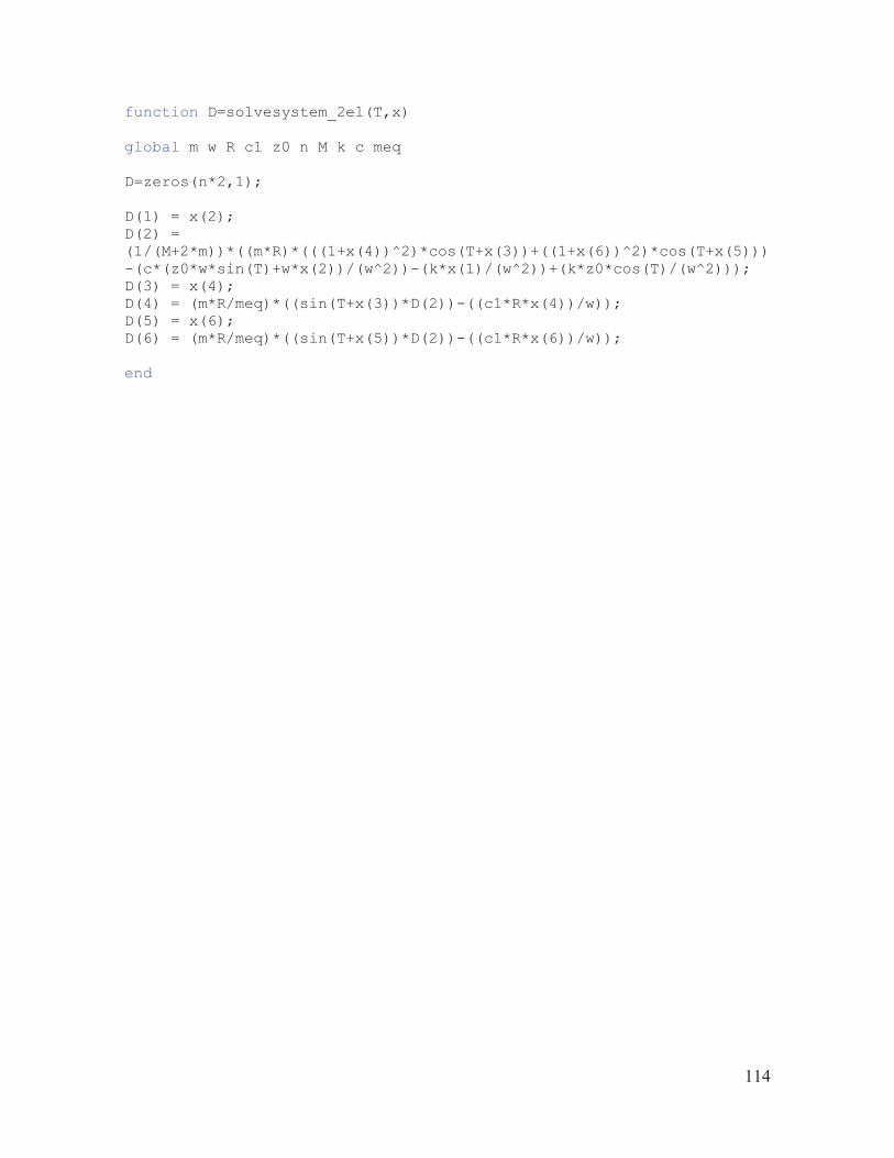
114
function D=solvesystem_2el(T,x) global m w R c1 z0 n M k c meq D=zeros(n*2,1); D(1) = x(2); D(2) = (1/(M+2*m))*((m*R)*(((1+x(4))^2)*cos(T+x(3))+((1+x(6))^2)*cos(T+x(5)))-(c*(z0*w*sin(T)+w*x(2))/(w^2))-(k*x(1)/(w^2))+(k*z0*cos(T)/(w^2))); D(3) = x(4); D(4) = (m*R/meq)*((sin(T+x(3))*D(2))-((c1*R*x(4))/w)); D(5) = x(6); D(6) = (m*R/meq)*((sin(T+x(5))*D(2))-((c1*R*x(6))/w)); end
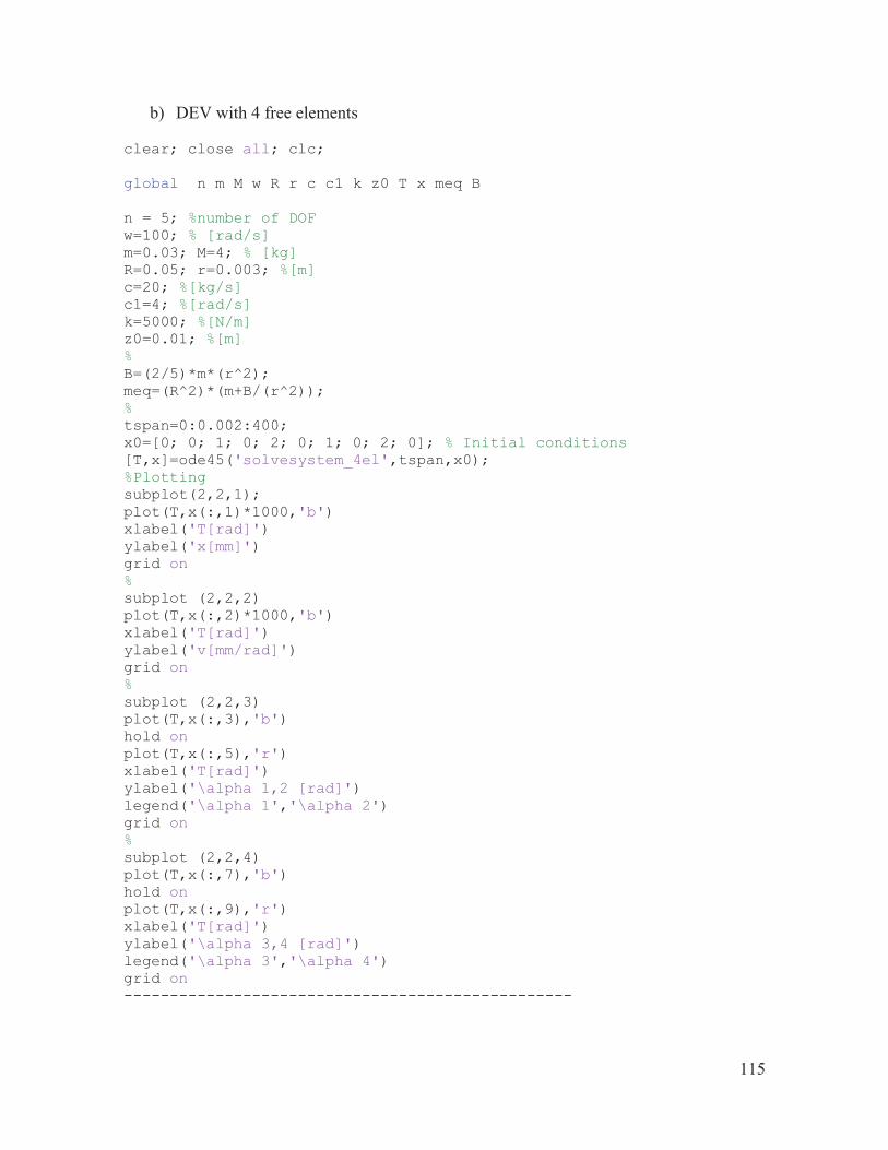
115
b) DEV with 4 free elements
clear; close all; clc; global n m M w R r c c1 k z0 T x meq B n = 5; %number of DOF w=100; % [rad/s] m=0.03; M=4; % [kg] R=0.05; r=0.003; %[m] c=20; %[kg/s] c1=4; %[rad/s] k=5000; %[N/m] z0=0.01; %[m] % B=(2/5)*m*(r^2); meq=(R^2)*(m+B/(r^2)); % tspan=0:0.002:400; x0=[0; 0; 1; 0; 2; 0; 1; 0; 2; 0]; % Initial conditions [T,x]=ode45('solvesystem_4el',tspan,x0); %Plotting subplot(2,2,1); plot(T,x(:,1)*1000,'b') xlabel('T[rad]') ylabel('x[mm]') grid on % subplot (2,2,2) plot(T,x(:,2)*1000,'b') xlabel('T[rad]') ylabel('v[mm/rad]') grid on % subplot (2,2,3) plot(T,x(:,3),'b') hold on plot(T,x(:,5),'r') xlabel('T[rad]') ylabel('\alpha 1,2 [rad]') legend('\alpha 1','\alpha 2') grid on % subplot (2,2,4) plot(T,x(:,7),'b') hold on plot(T,x(:,9),'r') xlabel('T[rad]') ylabel('\alpha 3,4 [rad]') legend('\alpha 3','\alpha 4') grid on -------------------------------------------------

116
function D=solvesystem_4el(T,x) global m w R c1 z0 n M k c meq D=zeros(n*2,1); D(1) = x(2); D(2) = (1/(M+4*m))*((m*R)*(((1+x(4))^2)*cos(T+x(3))+((1+x(6))^2)*cos(T+x(5))+((1+x(8))^2)*cos(T+x(7))+((1+x(10))^3)*cos(T+x(9)))-(c*(z0*w*sin(T)+w*x(2))/(w^2))-(k*x(1)/(w^2))+(k*z0*cos(T)/(w^2))); D(3) = x(4); D(4) = (m*R/meq)*((sin(T+x(3))*D(2))-((c1*R*x(4))/w)); D(5) = x(6); D(6) = (m*R/meq)*((sin(T+x(5))*D(2))-((c1*R*x(6))/w)); D(7) = x(8); D(8) = (m*R/meq)*((sin(T+x(7))*D(2))-((c1*R*x(8))/w)); D(9) = x(10); D(10) = (m*R/meq)*((sin(T+x(9))*D(2))-((c1*R*x(10))/w)); end

117
c) Inertial force clear; clc; close all; % %Parameters m=4.175; %[kg] c1=10; c2=5; %[kg/s] w=100; %[rad/s] k1=10000; k2=10000; %[N/m] % %Inertial force and phase angle equations phi=pi+atan(((c1+c2)*w)/(k1+k2-m*(w^2))) i=1; for alpha = -pi:0.001:3*pi/2 F1(i,1)=-0.5*(sin(alpha+phi)+sin(phi)); i=i+1; end % alpha = -pi:0.001:3*pi/2; plot(alpha,F1,'b') hold on ax = gca; ax.XAxisLocation = 'origin'; ax.YAxisLocation = 'origin'; box off %title ('Inertial Force Behaviour') xlabel ('\alpha [rad]') ylabel ('F [-]') % F=F1/amw^2 grid on %

118
d) Kinetics description of the rotary hammer internal components clear; close all; clc; clear; close all; clc; x0=5; % [mm] striker initial position v0=0; % [mm/s] striker initial velocity e=85; % [mm] striker max displacement a=10; % [mm] piston amplitude k1=0.7; % [-] restitution coef piston-striker k2=0.8; % [-] restitution coef striker-chisel w=100; %[rad/s] angular velocity of piston tf=3; % [s] simulation time m=0.075; % [kg] mass of the striker dt1=0.003; % [s] duration of piston-striker collision dt2=0.002; % [s] duration of striker-chisel collision %% Piston displacement functions z=@(t) a*sin(w*t); vz=@(t) a*w*cos(w*t); %% Functions of 1st collision with striker t1=(1/w)*asin(x0/a); %time for 1st impact (piston-striker) x1=x0; v1=vz(t1)*(1+k1)-v0*k1; %speed of striker after impact %% Functions of collision with chisel tC=@(t1,x1,vCm) t1+(e-x1)/vCm; %time for striker-chisel col. xC=e; vCp=@(vCm) -k2*vCm; %striker speed after col %% Functions of 2nd collision with piston (return of striker) cond=@(t2,v2) t2+(0.8*(e-a)/(abs(v2))); %ecc.init.cond. vMp=@(vz,vMm) vz*(1+k1)-vMm; %striker speed after col. %xMp=@(t) vz(t); numCol=1; T=zeros(2*numCol+1,1); X=zeros(2*numCol+1,1); V=zeros(2*numCol+1,1); F=zeros(2*numCol+1,1); i=1; T(1:3)=[0;t1;t1]; X(1:3)=[x0;x1;x1]; V(1:3)=[v0;v0;v1]; i=2;j=2; t3=0; while t3<tf t2=tC(T(i+1),X(i+1),V(i+1)); %t2 for impact with chisel v2=vCp(V(i+1)); %v2 after collision w/chisel T(i+2:i+3)=t2*[1;1]; %Assigns t2, bef&aft impact X(i+2:i+3)=xC*[1;1]; %Assigns pos. of impact w/chisel V(i+2:i+3)=[V(i+1);v2]; %Assigns striker speed b&a imp w/chisel F(j)=m*(V(i+1)-V(i))/(dt1*1000); F(j+1,1)=m*(V(i+1)-V(i+3))/(dt2*1000); fun=@(t3) a*sin(w*t3)-(v2*(t3-t2))-e; %t3 for 2nd impact striker-piston t3=fsolve(fun,cond(t2,v2)); T(i+4:i+5)=t3*[1;1]; %Assigns t3

119
X(i+4:i+5)=z(t3)*[1;1]; %Piston position for 2nd impact w/striker V(i+4:i+5)=[V(i+3);vMp(vz(t3),V(i+3))]; %Assigns speed bef&aft col. with piston %Special case: double collision piston-striker tcruce=(pi/w)*round(t3*w/pi); tlim=2*tcruce+pi/w-t3; fun1=@(t4) a*sin(w*t4)-(V(i+5)*(t4-t3))-X(i+5); t4=fsolve(fun1,tlim); if t4 > (t3+1e-8) T(i+6:i+7)=t4*[1;1]; X(i+6:i+7)=z(t4)*[1;1]; V(i+6:i+7)=[V(i+5);vMp(vz(t4),V(i+5))]; F(j+2)=-m*(V(i+6)-V(i+7))/(dt1*1000); i=i+6; j=j+3; numCol=numCol+3; else i=i+4; j=j+2; numCol=numCol+2; end end subplot (3,1,1) plot(T,X,'k'); xlabel 't [s]' ylabel 'X [mm]' title('Striker Impacts') hold on % Z=[]; j=1; tv = [0:0.01:t3]; for ti=[0:0.01:t3] Z(j,1)=a*sin(w*ti); j=j+1; end plot (tv,Z,'r'); grid on hold on xlim([0 3]) % subplot (3,1,2) plot(T,V,'k') xlabel 't [s]' ylabel 'V [mm/s]' xlim([0 3]) grid on % Time=zeros(numCol,1); h=1; while h<=numCol Time(h)=T(2*h-1); h=h+1; end

120
subplot(3,1,3) scatter (Time,F,'filled','k') xlabel 't [s]' ylabel 'F [N]' xlim([0 3]) grid on

121
e) Dynamic model of rotary hammer behaviour clear; clc; close all; global m1 m2 m3 k1 k2 k3 k4 z0 w n c1 c2 c3 c4 e0 n=3; %DOF m1=4.175; m2=0.075; m3=0.25; %[kg] k1=10000; k2=10000; k3=100000; k4=200000; %[N/m] z0=0.01; %[m] w=100; %[rad/s] c1=20; c2=5; c3=5; c4=2; %[kg/s] e0=0.02; %[m] tspan=0:0.001:3; x0=[0; 0; 0.004; 0; 0; 0]; [t,x]=ode45('HammerCompSolver',tspan,x0); F=Forces(t,x); %Plotting % Displacement x1 subplot (3,2,1) plot(t,x(:,1)*1000,'k') xlabel('t[s]') ylabel('x1[mm]') xlim([0 3]) ylim([-10 30]) grid on % Displacement x2 subplot (3,2,2) plot(t,x(:,3)*1000,'k') xlabel('t[s]') ylabel('x2[mm]') xlim([0 3]) ylim([-10 10]) grid on % Displacement x3 subplot (3,2,3) plot(t,x(:,5)*1000,'k') xlabel('t[s]') ylabel('x3[mm]') xlim([0 3]) ylim([-6 4]) grid on %Force F2 subplot (3,2,4) plot(t,F(:,2),'k') xlabel('t[s]') ylabel('F2[N]') xlim([0 3]) ylim([0 300]) grid on %Force F3

122
subplot (3,2,5) plot(t,F(:,3),'k') xlabel('t[s]') ylabel('F3[N]') xlim([0 3]) ylim([0 450]) grid on %Force F4 subplot (3,2,6) plot(t,F(:,4),'k') xlabel('t[s]') ylabel('F4[N]') xlim([0 3]) ylim([0 500]) grid on -------------------------------------------------
function D=HammerCompSolver(t,x) global m1 m2 m3 k1 k2 k3 k4 z0 w n c1 c2 c3 c4 e0 % x(1) = x1 x(2) = x1' % x(3) = x2 x(4) = x2' % x(5) = x3 x(6) = x3' D = zeros(n*2,1); z = z0*cos(w*t); zprim = -z0*w*sin(w*t); % F1=k1*(e0-x(1)); S1=c1*x(2); S2=c2*(x(2)+zprim-x(4)); S3=c3*(x(4)-x(6)); S4=c4*x(6); % F20=k2*(x(1)+z-x(3)); if F20>0 F2=F20; else F2=0; end % F30=k3*(x(3)-x(5)); S3=c3*(x(4)-x(6)); if F30>0 F3=F30; else F3=0; end % F40=k4*x(5); if F40>0 F4=F40; else F4=0;
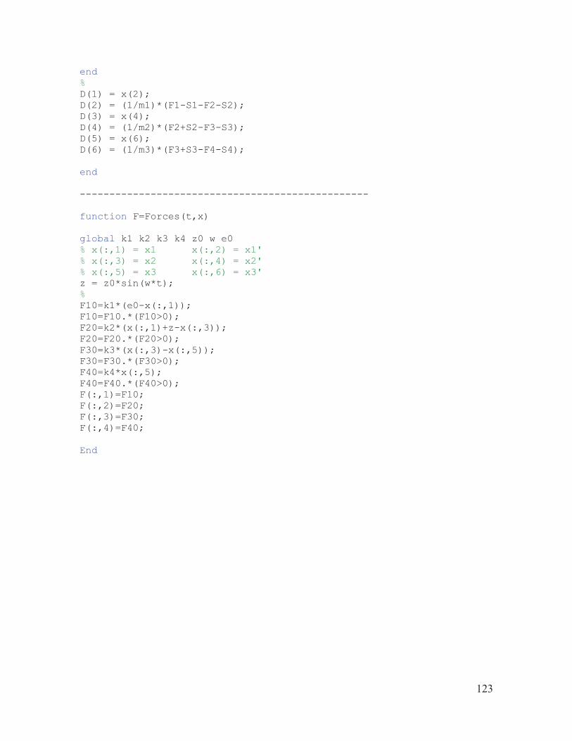
123
end % D(1) = x(2); D(2) = (1/m1)*(F1-S1-F2-S2); D(3) = x(4); D(4) = (1/m2)*(F2+S2-F3-S3); D(5) = x(6); D(6) = (1/m3)*(F3+S3-F4-S4); end -------------------------------------------------
function F=Forces(t,x) global k1 k2 k3 k4 z0 w e0 % x(:,1) = x1 x(:,2) = x1' % x(:,3) = x2 x(:,4) = x2' % x(:,5) = x3 x(:,6) = x3' z = z0*sin(w*t); % F10=k1*(e0-x(:,1)); F10=F10.*(F10>0); F20=k2*(x(:,1)+z-x(:,3)); F20=F20.*(F20>0); F30=k3*(x(:,3)-x(:,5)); F30=F30.*(F30>0); F40=k4*x(:,5); F40=F40.*(F40>0); F(:,1)=F10; F(:,2)=F20; F(:,3)=F30; F(:,4)=F40; End

124
f) Implementation of DEV to rotary hammer - unidirectional analysis
clear; close all; clc; global n w z0 mb m1 m2 m3 R r c1 c2 c3 c4 cR k1 k2 k3 k4 meq B T x e0 %Faltan términos de a'' n=7; %number of independent DOF w=100; % [rad/s] z0=0.01; %[m] Piston amplitude e0=0.02; %[m] mb=0.05; m1=4.175; m2=0.075; m3=0.25; % [kg] R=0.05; r=0.0115; %[m] c1=20; c2=5; c3=5; c4=2; %[kg/s] cR=2; %[1/s] k1=10000; k2=10000; k3=100000; k4=200000; %[N/m] % B=(2/5)*mb*(r^2); meq=(R^2)*(mb+B/(r^2)); % tspan=0:0.025:700; x0=[0.005; 0; 2.8; 0; 3.2; 0; 2.8; 0; 3.2; 0; 0.004; 0; 0; 0]; % Initial conditions Zeta=z0*cos(tspan); % [T,x]=ode45('SolveSyst_X',tspan,x0); F=Forces_X(T,x); % %Plotting figure(1) subplot(3,2,1); plot(T,x(:,1)*1000,'k') xlabel('T[rad]') ylabel('x1[mm]') xlim ([0 700]) grid on % subplot(3,2,2); plot(T,x(:,11)*1000,'k') xlabel('T[rad]') ylabel('x2[mm]') xlim ([0 700]) ylim ([-5 10]) grid on % subplot(3,2,3); plot(T,x(:,13)*1000,'k') xlabel('T[rad]') ylabel('x3[mm]') xlim ([0 700]) grid on % subplot (3,2,5) plot(T,x(:,3),'r') hold on plot(T,x(:,5),'k')

125
xlabel('T[rad]') ylabel('\alpha 1,2 [rad]') legend('\alpha 1','\alpha 2') xlim ([0 700]) grid on % subplot (3,2,6) plot(T,x(:,7),'r') hold on plot(T,x(:,9),'k') xlabel('T[rad]') ylabel('\alpha 3,4 [rad]') legend('\alpha 3','\alpha 4') xlim ([0 700]) grid on % figure(2) subplot (2,2,1) plot(T,F(:,1),'k') xlabel('T[rad]') ylabel('F1[N]') xlim ([0 700]) grid on % subplot (2,2,2) plot(T,F(:,2),'k') xlabel('T[rad]') ylabel('F2[N]') xlim ([0 700]) grid on % subplot (2,2,3) plot(T,F(:,3),'k') xlabel('T[rad]') ylabel('F3[N]') xlim ([0 700]) grid on % subplot (2,2,4) plot(T,F(:,4),'k') xlabel('T[rad]') ylabel('F4[N]') xlim ([0 700]) grid on hold on % -------------------------------------------------
function D=SolveSyst_X(T,x) global w R z0 n mb m1 m2 m3 c1 c2 c3 c4 cR meq k1 k2 k3 k4 e0 % x(1) = x1 x(2) = x1' % x(9) = a4 x(10) = a4' % x(3) = a1 x(4) = a1' % x(11) = x2 x(12) = x2' % x(5) = a2 x(6) = a2' % x(13) = x3 x(14) = x3' % x(7) = a3 x(8) = a3' % D=zeros(n*2,1);

126
% z = z0*cos(T); zprim = -z0*sin(T); F1=k1*(e0-x(1)); S1=c1*x(2); S2=c2*(x(2)+zprim-x(12)); S3=c3*(x(12)-x(14)); S4=c4*x(14); % F20=k2*(x(1)+z-x(11)); if F20>0 F2=F20; else F2=0; end F30=k3*(x(11)-x(13)); if F30>0 F3=F30; else F3=0; end F40=k4*x(13); if F40>0 F4=F40; else F4=0; end % D(1) = x(2); D(2) = (1/(m1+4*mb))*((-mb*R*(((1+x(4))^2)*cos(T+x(3))+((1+x(6))^2)* cos(T+x(5))+((1+x(8))^2)*cos(T+x(7))+((1+x(10))^3)*cos(T+x(9))))+(F1-(S1*w)-F2-(S2*w))/(w^2)); D(3) = x(4); D(4) = (mb*R/meq)*((-sin(T+x(3))*D(2))-((cR*R*x(4))/w)); D(5) = x(6); D(6) = (mb*R/meq)*((-sin(T+x(5))*D(2))-((cR*R*x(6))/w)); D(7) = x(8); D(8) = (mb*R/meq)*((-sin(T+x(7))*D(2))-((cR*R*x(8))/w)); D(9) = x(10); D(10) = (mb*R/meq)*((-sin(T+x(9))*D(2))-((cR*R*x(10))/w)); D(11) = x(12); D(12) = (1/(m2*(w^2)))*(F2+(S2*w)-F3-(S3*w)); D(13) = x(14); D(14) = (1/(m3*(w^2)))*(F3+(S3*w)-F4-(S4*w)); end -------------------------------------------------
function F=Forces_X(T,x) global k1 k2 k3 k4 z0 e0 % x(:,1) = x1 x(:,2) = x1' % x(:,11) = x2 x(:,12) = x2' % x(:,13) = x3 x(:,14) = x3' z = z0*cos(T); % F10=k1*(e0-x(:,1)); F10=F10.*(F10>0);
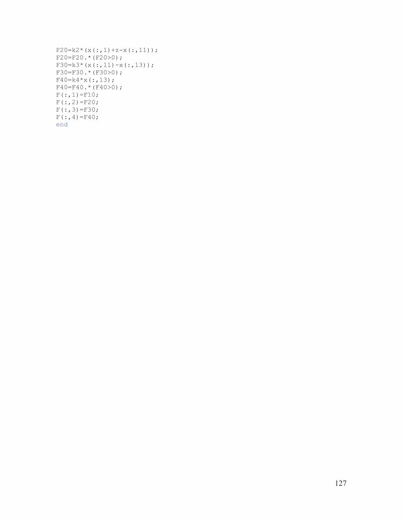
127
F20=k2*(x(:,1)+z-x(:,11)); F20=F20.*(F20>0); F30=k3*(x(:,11)-x(:,13)); F30=F30.*(F30>0); F40=k4*x(:,13); F40=F40.*(F40>0); F(:,1)=F10; F(:,2)=F20; F(:,3)=F30; F(:,4)=F40; end
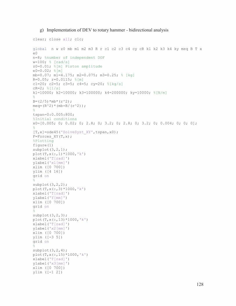
128
g) Implementation of DEV to rotary hammer - bidirectional analysis clear; close all; clc; global n w z0 mb m1 m2 m3 R r c1 c2 c3 c4 cy cR k1 k2 k3 k4 ky meq B T x e0 n=8; %number of independent DOF w=100; % [rad/s] z0=0.01; %[m] Piston amplitude e0=0.02; %[m] mb=0.07; m1=4.175; m2=0.075; m3=0.25; % [kg] R=0.05; r=0.0115; %[m] c1=20; c2=5; c3=5; c4=5; cy=20; %[kg/s] cR=2; %[1/s] k1=10000; k2=10000; k3=100000; k4=200000; ky=10000; %[N/m] % B=(2/5)*mb*(r^2); meq=(R^2)*(mb+B/(r^2)); % tspan=0:0.005:800; %Initial conditions x0=[0.005; 0; 0.02; 0; 2.8; 0; 3.2; 0; 2.8; 0; 3.2; 0; 0.004; 0; 0; 0]; % [T,x]=ode45('SolveSyst_XY',tspan,x0); F=Forces_XY(T,x); %Plotting figure(1) subplot(3,2,1); plot(T,x(:,1)*1000,'k') xlabel('T[rad]') ylabel('x1[mm]') xlim ([0 700]) ylim ([4 16]) grid on % subplot(3,2,2); plot(T,x(:,3)*1000,'k') xlabel('T[rad]') ylabel('Y[mm]') xlim ([0 700]) grid on % subplot(3,2,3); plot(T,x(:,13)*1000,'k') xlabel('T[rad]') ylabel('x2[mm]') xlim ([0 700]) ylim ([-3 5]) grid on % subplot(3,2,4); plot(T,x(:,15)*1000,'k') xlabel('T[rad]') ylabel('x3[mm]') xlim ([0 700]) ylim ([-1 2])

129
grid on % subplot (3,2,5) plot(T,x(:,5),'r') hold on plot(T,x(:,7),'k') xlabel('T[rad]') ylabel('\alpha 1,2 [rad]') legend('\alpha 1','\alpha 2') xlim ([0 700]) ylim ([-1 5]) grid on % subplot (3,2,6) plot(T,x(:,9),'r') hold on plot(T,x(:,11),'k') xlabel('T[rad]') ylabel('\alpha 3,4 [rad]') legend('\alpha 3','\alpha 4') xlim ([0 700]) ylim ([-1 5]) grid on % figure(2) subplot (2,2,1) plot(T,F(:,1),'k') xlabel('T[rad]') ylabel('F1[N]') xlim ([0 700]) ylim ([40 160]) grid on % subplot (2,2,2) plot(T,F(:,2),'k') xlabel('T[rad]') ylabel('F2[N]') xlim ([0 700]) ylim ([0 250]) grid on % subplot (2,2,3) plot(T,F(:,3),'k') xlabel('T[rad]') ylabel('F3[N]') xlim ([0 700]) ylim ([0 400]) grid on % subplot (2,2,4) plot(T,F(:,4),'k') xlabel('T[rad]') ylabel('F4[N]') xlim ([0 700]) grid on hold on -------------------------------------------------

130
function D=SolveSyst_XY(T,x) global w R z0 n mb m1 m2 m3 c1 c2 c3 c4 cR cy meq k1 k2 k3 k4 ky e0 % x(1) = x1 x(2) = x1' % x(9) = a3 x(10) = a3' % x(3) = y1 x(4) = y1' % x(11) = a4 x(12) = a4' % x(5) = a1 x(6) = a1' % x(13) = x2 x(14) = x2' % x(7) = a2 x(8) = a2' % x(15) = x3 x(16) = x3' % D=zeros(n*2,1); % z = z0*cos(T); zprim = -z0*sin(T); % F1=k1*(e0-x(1)); Fy=ky*x(3); S1=c1*x(2); S2=c2*(x(2)+zprim-x(14)); S3=c3*(x(14)-x(16)); S4=c4*x(16); Sy=cy*x(4); % F20=k2*(x(1)+z-x(13)); if F20>0 F2=F20; else F2=0; end F30=k3*(x(13)-x(15)); if F30>0 F3=F30; else F3=0; end F40=k4*x(15); if F40>0 F4=F40; else F4=0; end % D(1) = x(2); D(2) = (1/(m1+4*mb))*((-mb*R*(((1+x(6))^2)*cos(T+x(5))+((1+x(8))^2)*cos(T+x(7))+((1+x(10))^2)*cos(T+x(9))+((1+x(12))^3)*cos(T+x(11))))+(F1-(S1*w)-F2-(S2*w))/(w^2)); D(3) = x(4); D(4) = (1/(m1+4*mb))*((mb*R*(((1+x(6))^2)*sin(T+x(5))+((1+x(8))^2)*sin(T+x(7))-((1+x(10))^2)*sin(T+x(9))-((1+x(12))^3)*sin(T+x(11))))-Fy/(w^2)-Sy/w); D(5) = x(6); D(6) = (mb*R/meq)*(-D(2)*sin(T+x(5))-D(4)*cos(T+x(5))-(cR*R*x(6)/w)); D(7) = x(8); D(8) = (mb*R/meq)*(-D(2)*sin(T+x(7))-D(4)*cos(T+x(7))-(cR*R*x(8)/w)); D(9) = x(10); D(10) = (mb*R/meq)*(-D(2)*sin(T+x(9))+D(4)*cos(T+x(9))-(cR*R*x(10)/w)); D(11) = x(12); D(12) = (mb*R/meq)*(-D(2)*sin(T+x(11))+D(4)*cos(T+x(11))-(cR*R*x(12)/w)); D(13) = x(14);
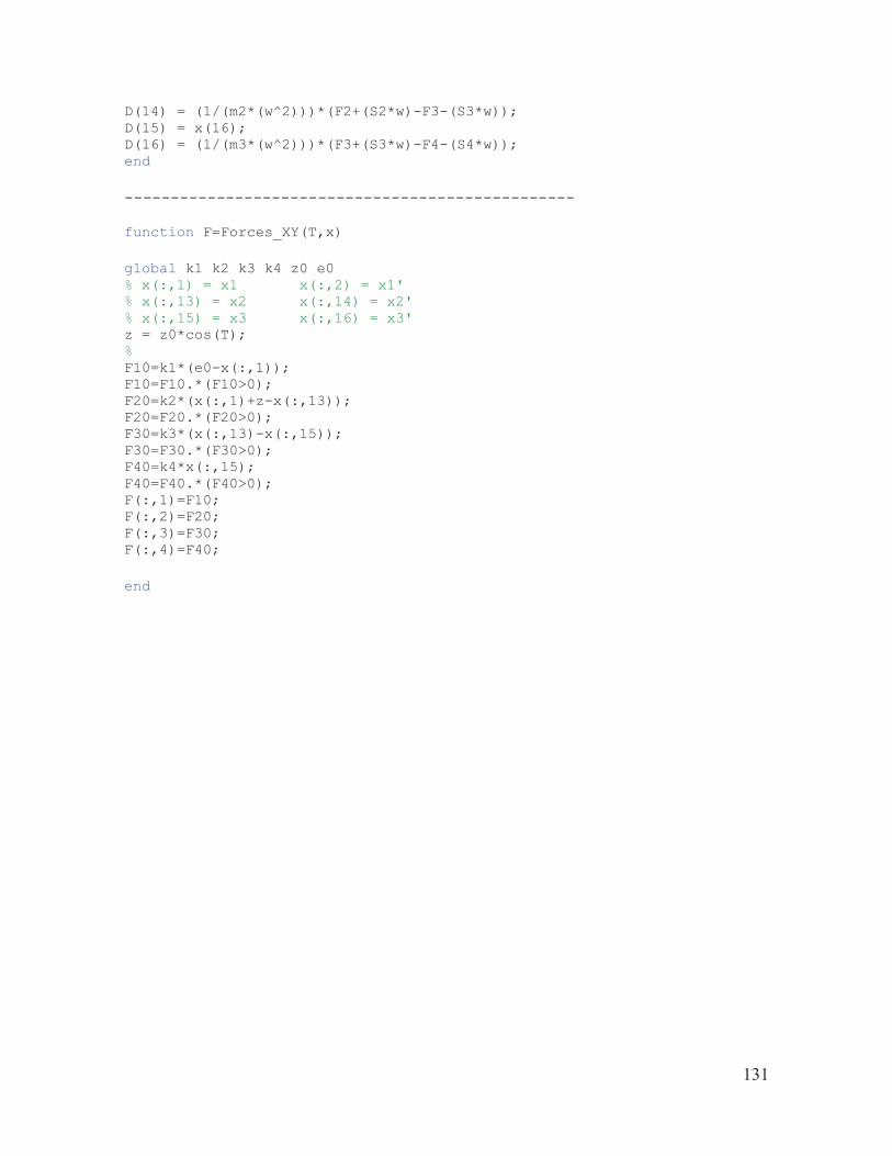
131
D(14) = (1/(m2*(w^2)))*(F2+(S2*w)-F3-(S3*w)); D(15) = x(16); D(16) = (1/(m3*(w^2)))*(F3+(S3*w)-F4-(S4*w)); end -------------------------------------------------
function F=Forces_XY(T,x) global k1 k2 k3 k4 z0 e0 % x(:,1) = x1 x(:,2) = x1' % x(:,13) = x2 x(:,14) = x2' % x(:,15) = x3 x(:,16) = x3' z = z0*cos(T); % F10=k1*(e0-x(:,1)); F10=F10.*(F10>0); F20=k2*(x(:,1)+z-x(:,13)); F20=F20.*(F20>0); F30=k3*(x(:,13)-x(:,15)); F30=F30.*(F30>0); F40=k4*x(:,15); F40=F40.*(F40>0); F(:,1)=F10; F(:,2)=F20; F(:,3)=F30; F(:,4)=F40; end

132
h) Dynamic model of rotary hammer with chisel chuck spring clear; clc; close all; global m1 m2 m3 k1 k2 k3 k4 z0 w n c1 c2 c3 c4 e0 k51 k52 n=3; %DOF m1=4.175; m2=0.075; m3=0.25; %[kg] k1=10000; k2=10000; k3=100000; k4=200000; %[N/m] k51=2000; k52=100; %[N/m] z0=0.01; %[m] w=100; %[rad/s] c1=20; c2=5; c3=5; c4=2; %[kg/s] e0=0.02; %[m] tspan=0:0.001:3; x0=[0; 0; 0.004; 0; 0; 0]; [t,x]=ode45('SolverChuck',tspan,x0); F=ForcesChuck(t,x); %Plotting % Displacement x1 figure(1) subplot (3,1,1) plot(t,x(:,1)*1000,'k') xlabel('t [s]') ylabel('x1 [mm]') xlim([0 1.6]) ylim([-10 25]) grid on % Displacement x2 subplot (3,1,2) plot(t,x(:,3)*1000,'k') xlabel('t [s]') ylabel('x2 [mm]') xlim([0 1.6]) ylim([-15 15]) grid on % Displacement x3 subplot (3,1,3) plot(t,x(:,5)*1000,'k') xlabel('t [s]') ylabel('x3 [mm]') xlim([0 1.6]) ylim([-10 5]) grid on % figure(2) %Force F2 subplot (2,2,1) plot(t,F(:,2),'k') xlabel('t [s]') ylabel('F2 [N]') xlim([0 1.6])

133
grid on %Force F3 subplot (2,2,2) plot(t,F(:,3),'k') xlabel('t [s]') ylabel('F3 [N]') xlim([0 1.6]) ylim([0 500]) grid on %Force F4 subplot (2,2,3) plot(t,F(:,4),'k') xlabel('t [s]') ylabel('F4 [N]') xlim([0 1.6]) grid on % subplot (2,2,4) plot(t,F(:,5),'k') xlabel('t [s]') ylabel('F5 [N]') xlim ([0 1.6]) ylim ([-10 150]) grid on hold on -------------------------------------------------
function D=SolverChuck(t,x) global m1 m2 m3 k1 k2 k3 k4 z0 w n c1 c2 c3 c4 e0 k51 k52 % x(1) = x1 x(2) = x1' % x(3) = x2 x(4) = x2' % x(5) = x3 x(6) = x3' D = zeros(n*2,1); z = z0*cos(w*t); zprim = -z0*w*sin(w*t); % F1=k1*(e0-x(1)); S1=c1*x(2); S2=c2*(x(2)+zprim-x(4)); S3=c3*(x(4)-x(6)); S4=c4*x(6); % F20=k2*(x(1)+z-x(3)); if F20>0 F2=F20; else F2=0; end % F30=k3*(x(3)-x(5)); S3=c3*(x(4)-x(6)); if F30>0 F3=F30; else
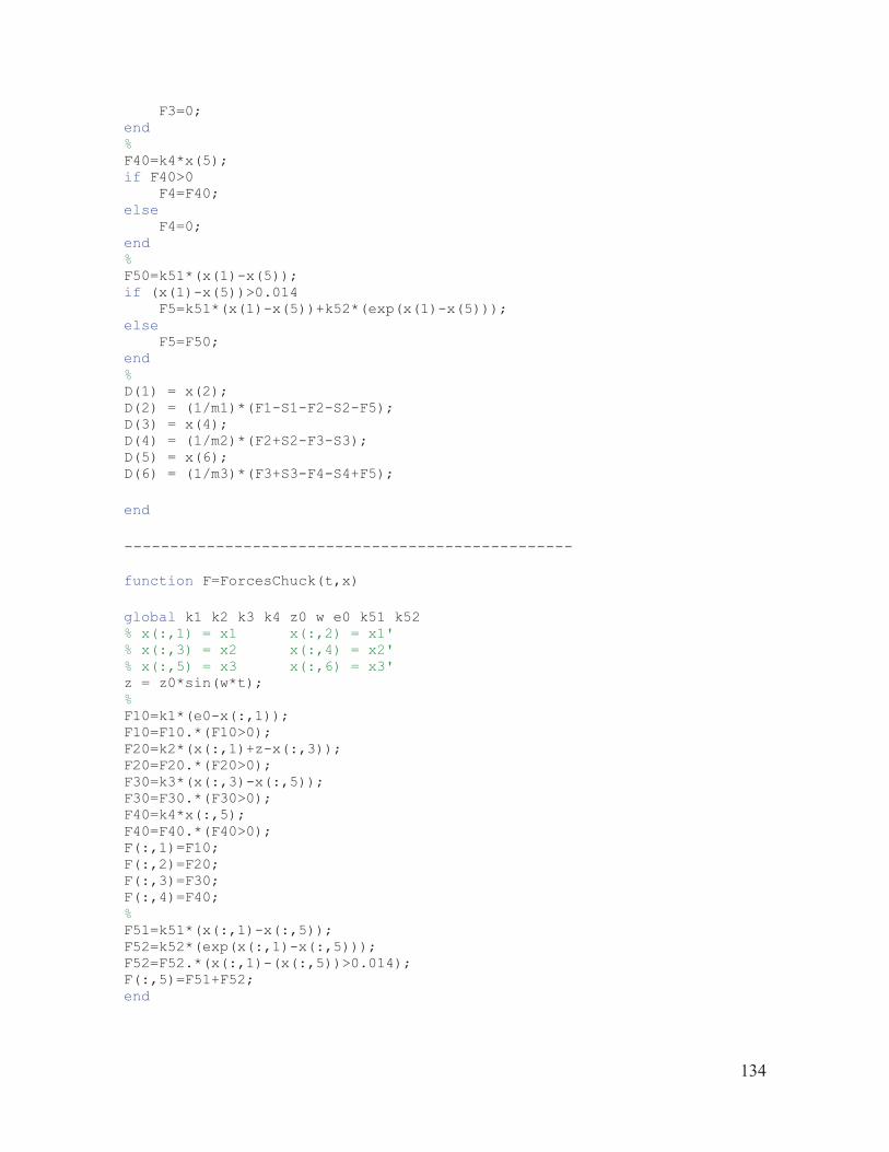
134
F3=0; end % F40=k4*x(5); if F40>0 F4=F40; else F4=0; end % F50=k51*(x(1)-x(5)); if (x(1)-x(5))>0.014 F5=k51*(x(1)-x(5))+k52*(exp(x(1)-x(5))); else F5=F50; end % D(1) = x(2); D(2) = (1/m1)*(F1-S1-F2-S2-F5); D(3) = x(4); D(4) = (1/m2)*(F2+S2-F3-S3); D(5) = x(6); D(6) = (1/m3)*(F3+S3-F4-S4+F5); end -------------------------------------------------
function F=ForcesChuck(t,x) global k1 k2 k3 k4 z0 w e0 k51 k52 % x(:,1) = x1 x(:,2) = x1' % x(:,3) = x2 x(:,4) = x2' % x(:,5) = x3 x(:,6) = x3' z = z0*sin(w*t); % F10=k1*(e0-x(:,1)); F10=F10.*(F10>0); F20=k2*(x(:,1)+z-x(:,3)); F20=F20.*(F20>0); F30=k3*(x(:,3)-x(:,5)); F30=F30.*(F30>0); F40=k4*x(:,5); F40=F40.*(F40>0); F(:,1)=F10; F(:,2)=F20; F(:,3)=F30; F(:,4)=F40; % F51=k51*(x(:,1)-x(:,5)); F52=k52*(exp(x(:,1)-x(:,5))); F52=F52.*(x(:,1)-(x(:,5))>0.014); F(:,5)=F51+F52; end

135
i) Implementation of DEV to the rotary hammer dynamic model with chuck spring clear; close all; clc; global n w z0 mb m1 m2 m3 R r c1 c2 c3 c4 cy cR k1 k2 k3 k4 ky meq B T x e0 k51 k52 n=8; %number of independent DOF w=100; % [rad/s] z0=0.01; %[m] e0=0.02; %[m] mb=0.1; m1=4.175; m2=0.075; m3=0.25; % [kg] R=0.05; r=0.0145; %[m] c1=20; c2=5; c3=5; c4=5; cy=20; %[kg/s] cR=4; %[1/s] k1=10000; k2=10000; k3=100000; k4=200000; ky=10000; %[N/m] k51=2000; k52=100; %[N/m] % B=(2/5)*mb*(r^2); meq=(R^2)*(mb+B/(r^2)); % tspan=0:0.005:600; x0=[0.005; 0; 0.02; 0; 2.8; 0; 3.2; 0; 2.8; 0; 3.2; 0; 0.001; 0; 0.002; 0]; % Initial conditions % [T,x]=ode45('SolveSyst_chuck',tspan,x0); F=Forces_chuck(T,x); % %Plotting figure(1) subplot(3,2,1); plot(T,x(:,1)*1000,'k') xlabel('\tau [rad]') ylabel('x1[mm]') %xlim ([0 500]) %ylim ([4 16]) grid on % subplot(3,2,2); plot(T,x(:,3)*1000,'k') xlabel('\tau [rad]') ylabel('Y[mm]') xlim ([0 500]) grid on % subplot(3,2,3); plot(T,x(:,13)*1000,'k') xlabel('\tau [rad]') ylabel('x2[mm]') xlim ([0 500]) %ylim ([-3 5]) grid on % subplot(3,2,4); plot(T,x(:,15)*1000,'k')

136
xlabel('\tau [rad]') ylabel('x3[mm]') xlim ([0 500]) %ylim ([-1 2]) grid on % subplot (3,2,5) plot(T,x(:,5),'r') hold on plot(T,x(:,7),'k') xlabel('\tau [rad]') ylabel('\alpha 1,2 [rad]') legend('\alpha 1','\alpha 2') xlim ([0 500]) %ylim ([-1 5]) grid on % subplot (3,2,6) plot(T,x(:,9),'r') hold on plot(T,x(:,11),'k') xlabel('\tau [rad]') ylabel('\alpha 3,4 [rad]') legend('\alpha 3','\alpha 4') xlim ([0 500]) %ylim ([-1 5]) grid on % figure(2) subplot (3,2,1) plot(T,F(:,1),'k') xlabel('\tau [rad]') ylabel('F1[N]') xlim ([0 400]) %ylim ([40 160]) grid on % subplot (3,2,2) plot(T,F(:,2),'k') xlabel('\tau [rad]') ylabel('F2[N]') xlim ([0 200]) %ylim ([0 250]) grid on % subplot (3,2,3) plot(T,F(:,3),'k') xlabel('\tau [rad]') ylabel('F3[N]') xlim ([0 200]) %ylim ([0 400]) grid on % subplot (3,2,4) plot(T,F(:,4),'k') xlabel('\tau [rad]') ylabel('F4[N]')

137
xlim ([0 200]) grid on hold on % subplot (3,2,5) plot(T,F(:,5),'k') xlabel('\tau [rad]') ylabel('F5[N]') xlim ([0 200]) ylim ([0 150]) grid on hold on % subplot(3,2,6) plot(T,(x(:,1)-x(:,15))*1000,'k') xlabel ('\tau [rad]') ylabel ('x1-x3[mm]') xlim ([0 400]) grid on hold on -------------------------------------------------
function D=SolveSyst_chuck(T,x) global w R z0 n mb m1 m2 m3 c1 c2 c3 c4 cR cy meq k1 k2 k3 k4 ky e0 k51 k52 % x(1) = x1 x(2) = x1' % x(9) = a3 x(10) = a3' % x(3) = y1 x(4) = y1' % x(11) = a4 x(12) = a4' % x(5) = a1 x(6) = a1' % x(13) = x2 x(14) = x2' % x(7) = a2 x(8) = a2' % x(15) = x3 x(16) = x3' % D=zeros(n*2,1); % z = z0*cos(T); zprim = -z0*sin(T); % F1=k1*(e0-x(1)); Fy=ky*x(3); S1=c1*x(2); S2=c2*(x(2)+zprim-x(14)); S3=c3*(x(14)-x(16)); S4=c4*x(16); Sy=cy*x(4); % F20=k2*(x(1)+z-x(13)); if F20>0 F2=F20; else F2=0; end F30=k3*(x(13)-x(15)); if F30>0 F3=F30; else F3=0;
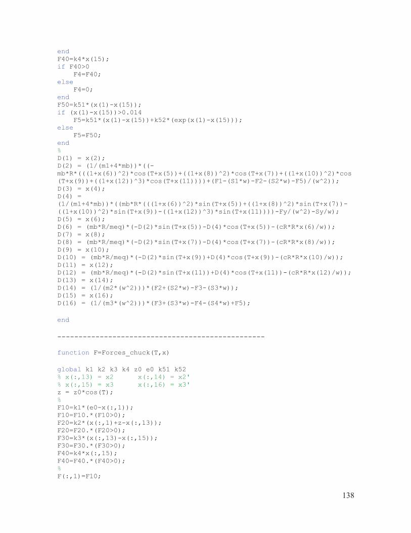
138
end F40=k4*x(15); if F40>0 F4=F40; else F4=0; end F50=k51*(x(1)-x(15)); if (x(1)-x(15))>0.014 F5=k51*(x(1)-x(15))+k52*(exp(x(1)-x(15))); else F5=F50; end % D(1) = x(2); D(2) = (1/(m1+4*mb))*((-mb*R*(((1+x(6))^2)*cos(T+x(5))+((1+x(8))^2)*cos(T+x(7))+((1+x(10))^2)*cos(T+x(9))+((1+x(12))^3)*cos(T+x(11))))+(F1-(S1*w)-F2-(S2*w)-F5)/(w^2)); D(3) = x(4); D(4) = (1/(m1+4*mb))*((mb*R*(((1+x(6))^2)*sin(T+x(5))+((1+x(8))^2)*sin(T+x(7))-((1+x(10))^2)*sin(T+x(9))-((1+x(12))^3)*sin(T+x(11))))-Fy/(w^2)-Sy/w); D(5) = x(6); D(6) = (mb*R/meq)*(-D(2)*sin(T+x(5))-D(4)*cos(T+x(5))-(cR*R*x(6)/w)); D(7) = x(8); D(8) = (mb*R/meq)*(-D(2)*sin(T+x(7))-D(4)*cos(T+x(7))-(cR*R*x(8)/w)); D(9) = x(10); D(10) = (mb*R/meq)*(-D(2)*sin(T+x(9))+D(4)*cos(T+x(9))-(cR*R*x(10)/w)); D(11) = x(12); D(12) = (mb*R/meq)*(-D(2)*sin(T+x(11))+D(4)*cos(T+x(11))-(cR*R*x(12)/w)); D(13) = x(14); D(14) = (1/(m2*(w^2)))*(F2+(S2*w)-F3-(S3*w)); D(15) = x(16); D(16) = (1/(m3*(w^2)))*(F3+(S3*w)-F4-(S4*w)+F5); end -------------------------------------------------
function F=Forces_chuck(T,x) global k1 k2 k3 k4 z0 e0 k51 k52 % x(:,13) = x2 x(:,14) = x2' % x(:,15) = x3 x(:,16) = x3' z = z0*cos(T); % F10=k1*(e0-x(:,1)); F10=F10.*(F10>0); F20=k2*(x(:,1)+z-x(:,13)); F20=F20.*(F20>0); F30=k3*(x(:,13)-x(:,15)); F30=F30.*(F30>0); F40=k4*x(:,15); F40=F40.*(F40>0); % F(:,1)=F10;

139
F(:,2)=F20; F(:,3)=F30; F(:,4)=F40; % F51=k51*(x(:,1)-x(:,15)); F52=k52*(exp(x(:,1)-x(:,15))); F52=F52.*(x(:,1)-(x(:,15))>0.014); F(:,5)=F51+F52; end
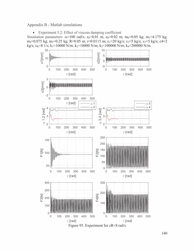
140
Appendix B - Matlab simulations
� Experiment 5.2: Effect of viscous damping coefficient Simulation parameters: ω=100 rad/s; z0=0.01 m; e0=0.02 m; mb=0.05 kg; m1=4.175 kg; m2=0.075 kg; m3=0.25 kg; R=0.05 m; r=0.0115 m; c1=20 kg/s; c2=5 kg/s; c3=5 kg/s; c4=2 kg/s; cR=8 1/s; k1=10000 N/m; k2=10000 N/m; k3=100000 N/m; k4=200000 N/m.
Figure 95. Experiment for cR=8 rad/s
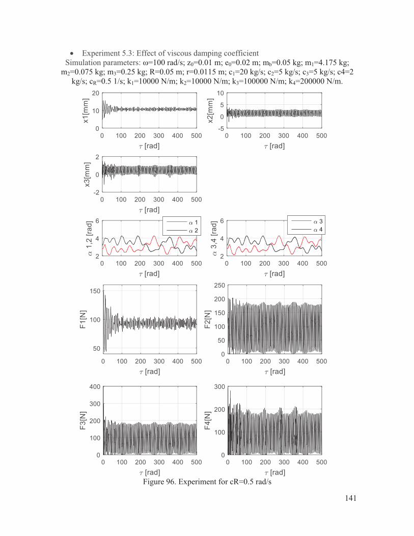
141
� Experiment 5.3: Effect of viscous damping coefficient Simulation parameters: ω=100 rad/s; z0=0.01 m; e0=0.02 m; mb=0.05 kg; m1=4.175 kg;
m2=0.075 kg; m3=0.25 kg; R=0.05 m; r=0.0115 m; c1=20 kg/s; c2=5 kg/s; c3=5 kg/s; c4=2 kg/s; cR=0.5 1/s; k1=10000 N/m; k2=10000 N/m; k3=100000 N/m; k4=200000 N/m.
Figure 96. Experiment for cR=0.5 rad/s
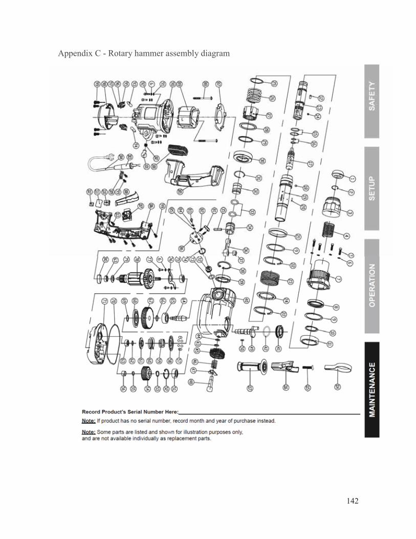
142
Appendix C - Rotary hammer assembly diagram

143

144
REFERENCES Amazon Services LLC Associate Program. (2018). The Essential List of the Different Types of Power Tools. Retrieved June 12, 2018 from Amzaon Services: https://toolconsult.com/guides/different-power-tool-types-list#hammer-drill
Bosch. (2018). Cordless Hammer Drill / Drivers. Retrieved June 14, 2018, from Bosch Power Tools: https://www.boschtools.com/us/en/boschtools-ocs/hammer-drills-23516-c/
Bosch (2018). Bosch GSH 11 VC Professional Demolition hammer with SDS max. [Video]. Retrieved from https://www.youtube.com/watch?v=aO4PbdRdwqM
Brammer, A; Peterson, D. (2004). Vibration, Mechanical, Shock, and Impact. Chapter 10
British Standards Institution. (1987). Measurement and Evaluation of Human Exposure to Vibration Transmitted to the Hand. BS 6842. London: BSI.
Broch, J.T. (1972) The Application of the Bruel & Kjaer Measuring Systems to Mechanical Vibration and Shock Measurements (1st ed) New York: Nestle Company Inc.
Canadian Center of Ocupational Health and Safety. Government of Canada. (2018) Raynaud’s Phenomenon. Accessed on July 02: https://www.ccohs.ca/oshanswers/ diseases/raynaud.html
Castro, J., Palacios, M., García, G., & Moreno, L. (2014). Salud, Ambiente y Trabajo. México: McGraw Hill. P. 277
Centro de Acústica Aplicada, SL. (2009) “Estudio del Nivel de Exposición a Vibraciones Mecánicas en Diferentes Puestos de Trabajo” España: Ministerio de Trabajo e Inmigración de España. Accessed on June 15, 2018: http://www.oect.es/Observatorio/Contenidos/ InformesPropios/Desarrollados/Ficheros/Resumen%20Estudio%20Exposición%20Vibraciones%20Mecánicas.pdf
Dahl, T. (2016). Impact Driver. Popular Mechanics. Retrieved July 21, 2018 from: https://www.popularmechanics.com/home/tools/how-to/a18931/how-to-use-an-impact-driver-diy-projects/
Dewalt. (2018). Shocks Active Vibration Control. Retrieved June 25, 2018, from https://www.dewalt.com/jobsite-solutions/perform-and-protect/vibration
Dewalt (2018). Impact drivers and wrenches. Retrieved June 25, 2018, from https://www.dewalt.com/products/power-tools/impact-drivers-and-wrenches?pageNum=2
Discovery Channel. (2018). Demolitore Kombihammer Bohrhammer Milwaukee Kango 950S 950 S SDS MAX [Video]. Retrieved from https://www.youtube.com/watch?v=Xd9o2D2wmhA

145
Dupzyk, K. (2016). Jackhammer. Popular Mechanics, 193(1), 20-21.
Griffin, M. (2018). Cool Tools: Rotary Hammers. Electrical Contractor Magazine. Retrieved from https://www.ecmag.com/section/your-business/cool-tools-rotary-hammers
Hernández, F. G. (2012). Tratado de Medicina del trabajo. Introducción a la salud laboral, aspectos jurídicos y técnicos. Madrid: Ministerio de Trabajo y Asuntos Sociales. Vol I, II.
Ideara. (2014). Vibraciones Mecánicas. Factores relacionados con la fuente y medidas de control. España. Confederación de Empresarios de Pontevedra CEP. Retrieved June 16, 2018 from: https://idearainvestigacion.es/wp-content/uploads/2014/10/GUIA_ vibraciones-mecanicas_final_baixa-calidade.pdf
Inman, D. J. (2001) Engineering Vibration (2da ed.) New Jersey: Prentice Hall. P. 359
Majewski, T. (1987). Synchronous Vibration Eliminator for an Object Having One Degree of Freedom. Journal of Sound and Vibration, 112(3), 401-413.
Majewski, T. (2017). Vibraciones en sistemas físicos (Segunda ed.). México: Alfaomega.
Makita. (2015). Antivibrations systems AVT [Video]. Retrieved June 21, 2018, from https://www.youtube.com/watch?v=xmoHtY7yf2c
Makita UK. (2018). Antivibration technology. Retrieved June 21, 2018, from http://www.makitauk.com/anti-vibration-technology.html
Rao, S. (2011). Mechanical Vibrations (5th ed.). New Jersey: Prentice Hall.
The Essential List of the Different Types of Power Tools. (2018). Retrieved June 09, 2018 from https://toolconsult.com/guides/different-power-tool-types-list#hammer-drill
Thomson, William. (1988) Theory of Vibration with Applications (3rd ed.) New Jersey. Prentice Hall. P. 138
Walshaw, A.C. (1984) Mechanical Vibrations with Applications (1ra ed) New York: John Wiley and Sons. P. 108
What is a Hammer Drill vs Rotary Hammers. (2018). Family Handyman.
Woodford, C. (2017). Jackhammer / Pneumatic Drill. Retrieved June 12, 2018, from https://www.explainthatstuff.com/jackhammer.html
Yagid, R. (2009). Hammer Drill-Driver. Fine Home Building. Retrieved July 06, 2018 from: https://www.finehomebuilding.com/2009/11/12/hammer-drill-driver#