Embed Size (px)
Citation preview
UPTEC ES 11009
Examensarbete 15 hpMars 2011
Modelling of a Power System in a Combined Cycle Power Plant
Sara Bengtsson
Teknisk- naturvetenskaplig fakultet UTH-enheten Besöksadress: Ångströmlaboratoriet Lägerhyddsvägen 1 Hus 4, Plan 0 Postadress: Box 536 751 21 Uppsala Telefon: 018 – 471 30 03 Telefax: 018 – 471 30 00 Hemsida: http://www.teknat.uu.se/student
Abstract
Modelling of a Power System in a Combined CyclePower Plant
Sara Bengtsson
Simulators for power plants can be used for many different purposes, like training foroperators or for adjusting control systems, where the main objective is to perform arealistic behaviour for different operating conditions of the power plant. Due to anincreased amount of variable energy sources in the power system, the role of theoperators has become more important. It can therefore be very valuable for theoperators to try different operating conditions like island operation.
The aim of this thesis is to model the power system of a general combined-cyclepower plant simulator. The model should contain certain components and have arealistic behaviour but on the same time be simple enough to perform simulations inreal time. The main requirements are to simulate cold start, normal operation, trip ofgenerator, a controlled change-over to island operation and then resynchronisation.
The modelling and simulations are executed in the modelling software Dymola,version 6.1. The interface for the simulator is built in the program LabView, but thatis beyond the scope of this thesis.
The results show a reasonable performance of the power system with most of theobjectives fulfilled. The simulator is able to perform a start-up, normal load changes,trip of a generator, change-over to island operation as well as resynchronisation ofthe power plant to the external power grid. However, the results from thechanging-over to island operation, as well as large load losses during island operation,show an unreasonable behaviour of the system regarding the voltage magnitude atthat point. This is probably due to limitations in calculation capacity of Dymola, andthe problem has been left to further improvements due to lack of time.
There has also been a problem during the development of a variable speed regulatedinduction motor and it has not been possible to make it work due to lack of enoughknowledge about how Dymola is performing the calculations. Also this problem hasbeen left to further improvements due to lack of time.
ISSN: 1650-8300, UPTEC ES11 009Examinator: Kjell PernestålÄmnesgranskare: Urban LundinHandledare: Ramona Huuva

Sammanfattning Energiförsörjningen har under de senaste decennierna blivit en av de viktigaste frågorna i världen i
takt med att miljön, och framförallt växthuseffekten, tagits alltmer på allvar. På grund av detta har
även mängden förnyelsebara energikällor i vårt energisystem ökat. Många av de förnybara
energikällorna är väldigt varierande i sin energiproduktion, vilket ställer högre krav på regleringen
och därmed även på systemoperatörerna.
Kraftverkssimulatorer kan användas för olika syften, där en av de viktigaste är som
träningssimulatorer för kraftverksoperatörer. På Solvina AB har man under många år utvecklat olika
typer av träningssimulatorer för olika kraftverk, och då efterfrågan ökat ytterligare bestämde man sig
för att göra en generell simulatormodell som enkelt ska kunna anpassas till specifika anläggningar.
Syftet för det här projektet har varit att ta fram en elkraftsmodell över elsystemet i en generell
gaskombianläggning, som ett steg i utvecklingen av den generella simulatorn. Modellen var tvungen
att innehålla vissa specifika komponenter, och målet har varit att ha en flexibel modell med realistiskt
uppförande för olika driftsförhållanden. De huvudsakliga driftsförhållanden som simulatorn haft som
krav att kunna simulera är: kallstart av kraftverket, normaldrift, trip av en generator, normala
lastfrånslag, kontrollerad övergång till husturbindrift samt en återinfasning mot nätet.
För att få en uppfattning om olika kraftverksmodeller och simulatorer har bland annat ett
studiebesök på kraftvärmeverket i Uppsala genomförts.
Modelleringen och simuleringen har genomförts i modelleringsprogrammet Dymola, version 6.1.
Dymola har fördelen att kunna modellera stora, komplexa system både grafiskt och kodbaserat.
Själva simulatorns gränssnitt är skapat i Labview, men implementerandet av modellen i detta har
varit utanför projektets avgränsning.
Resultaten visar i de flesta fall tillfredsställande simuleringsresultat med de flesta målen uppfyllda.
Simulatorn kan genomföra de erforderliga driftsförhållandena relativt väl. Däremot är resultatet från
husturbinövergången och i övrigt stora lastfrånslag inte helt rimliga, vilket troligtvis beror på
begränsningar i Dymolas beräkningskapacitet och sätt att utföra beräkningarna. På grund av tidsbrist
har detta lämnats som förbättringsåtgärd.
Samma typ av problem uppstod då en modell över en varvtalsstyrd induktionsmotor skulle utvecklas.
Det har tyvärr inte gått att få denna modell att fungera, vilket beror på begränsning i kunskap om hur
Dymola genomför beräkningarna. Även detta problem har lämnats som en förbättringsåtgärd.

Nomenclature
Symbols
Symbol Description Value Unit
δ Load angle [rad]
E Resulting emf [V]
Ef Field voltage [V]
f Frequency [Hz]
H Inertia constant [s]
J Moment of inertia [kg*m2]
KD Damping factor [1]
n Turning ratio [1]
ns Synchronous speed [rpm]
p Number of pole pairs [1]
P Active power [W]
π Pi 3.14159265 [1]
Q Reactive power [VAr]
R Frequency characteristics [J]
Ra Armature resistance [Ω]
Rc Shunt resistance (count for power lost in core) [Ω]
s Slip [1]
S Apparent power [VA]
T Torque [Nm]
Vt Terminal voltage [V]
Xl Leakage reactance [Ω]
Xm Magnetising reactance [Ω]
Y G+jB, admittance [S]
Z R+jX=impedance [Ω]
ω Angular frequency/speed [rad/s]
ωs Synchronous angular speed 2π*50 [rad/s]
Table 0.1: Symbols from the report.
Acronyms
Acronym Description
AVR Automatic voltage regulator
DAE Differential algebraic equations
emf Electromagnetic force
mmf Magnetomotive force
ODE Ordinary differential equations
pu Per unit, e.g. Rpu=R/Rbase
TSO Transmission system operator
rms Root mean square
Table 0.2: Acronyms from the report.

Acknowledgments This thesis has been performed at Solvina AB in Gothenburg, as the last course of my Master of
Science in Energy System at Uppsala University and the Swedish University of Agricultural Science,
Uppsala. Examiner has been Kjell Pernestål, senior lecturer at the department of Physics and
Astronomy at Uppsala University.
This thesis would never have been written without all the help and support I have obtained, and
therefore I would like to thank the following people:
Ramona Huuva, supervisor at Solvina AB, for all help and guidance.
Bengt Johansson, Solvina AB, for your time and help with knowledge in all the technical questions.
Mikael Eriksson, Solvina AB, for your time, patience and help with Dymola.
Urban Lundin, reviewer and senior lecturer at the department of Engineering Science, Division of
Electricity at Uppsala University for time and support.
Additional employees at Solvina AB for a very nice time during my project time.
And of course my family, boyfriend and friends for all support and patience during this time!

1
Table of Contents Sammanfattning ...................................................................................................................................... 1
Nomenclature .......................................................................................................................................... 2
Acknowledgments ................................................................................................................................... 3
1. Introduction ..................................................................................................................................... 4
1.1 Background .............................................................................................................................. 4
1.2 Purpose and restrictions ......................................................................................................... 4
1.3 Limitations of the thesis .......................................................................................................... 5
1.4 Outline of the thesis ................................................................................................................ 6
2. Method ............................................................................................................................................ 7
2.1 Literature studies .................................................................................................................... 7
2.2 Study visit ................................................................................................................................ 7
2.3 Modelling ................................................................................................................................. 7
2.4 Simulations .............................................................................................................................. 7
2.4.1 Cold start of the system .................................................................................................. 8
2.4.2 Load changes during normal operation .......................................................................... 8
2.4.3 Trip of generator during normal operation ..................................................................... 8
2.4.4 Island operation ............................................................................................................... 8
2.4.5 Load change during island operation .............................................................................. 8
2.4.6 Synchronisation of the power plant to the external power grid ..................................... 8
3. Theory .............................................................................................................................................. 9
3.1 Simulators for power plants .................................................................................................... 9
3.2 Electric power system ............................................................................................................. 9
3.2.1 Electric power systems in general ................................................................................... 9
3.2.2 Components in the power system ................................................................................ 11
3.3 Island operation..................................................................................................................... 24
3.4 Control strategies .................................................................................................................. 25
3.5 Modelling program ................................................................................................................ 25
3.5.1 Modelica ........................................................................................................................ 25
3.5.2 Dymola ........................................................................................................................... 26
4. Reference power plants ................................................................................................................ 27
4.1 The combined power and heating plant in Uppsala ............................................................. 27
4.2 Södra Cell Mörrum ................................................................................................................ 27
2
5. Synthesised model of the power system ...................................................................................... 29
5.1 Overview of the model .......................................................................................................... 29
5.1.1 Power system model ..................................................................................................... 29
5.1.2 Control model ................................................................................................................ 31
5.2 The complexity of the model and computing time ............................................................... 32
5.3 Problems and limitations ....................................................................................................... 33
6. Models of components in the power system ................................................................................ 34
6.1 Generators ............................................................................................................................. 34
6.1.1 Synchronous generator ................................................................................................. 34
6.1.2 Excitation system ........................................................................................................... 36
6.1.3 Turbine governor ........................................................................................................... 37
6.1.4 Synchronisation controller ............................................................................................ 38
6.2 Transformers ......................................................................................................................... 38
6.2.1 Tap changer ................................................................................................................... 38
6.3 Loads ...................................................................................................................................... 38
6.4 Motors ................................................................................................................................... 39
6.4.1 Constant speed controlled induction motor ................................................................. 39
6.4.2 Variable speed controlled induction motor .................................................................. 40
6.5 Transmission net, breakers and shunt capacitors ................................................................. 41
6.5.1 Transmission line ........................................................................................................... 41
6.5.2 Breakers ......................................................................................................................... 41
6.5.3 Shunt capacitance ......................................................................................................... 42
6.6 Protection systems ................................................................................................................ 42
6.6.1 Current protection ......................................................................................................... 42
6.6.2 Voltage protection ......................................................................................................... 42
6.6.3 Frequency protection .................................................................................................... 42
6.6.4 Magnetisation protection .............................................................................................. 42
6.6.5 Reversed power protection ........................................................................................... 43
7. Results of simulations .................................................................................................................... 44
7.1 Validation of components ..................................................................................................... 44
7.1.1 Start-up of a constant speed controlled induction motor ............................................ 44
7.1.2 Start-up of a generator .................................................................................................. 46
7.1.3 Tap changing of a transformer ...................................................................................... 49
7.2 Validation of power system model ....................................................................................... 50
3
7.2.1 Cold start of the system ................................................................................................ 50
7.2.2 Load change during normal operation .......................................................................... 54
7.2.3 Trip of generator during normal operation ................................................................... 56
7.2.4 Island operation ............................................................................................................. 58
7.2.5 Load change during island operation ............................................................................ 60
7.2.6 Synchronisation of the power plant to the external power grid ................................... 63
8. Discussion ...................................................................................................................................... 65
9. Conclusions and further research ................................................................................................. 67
9.1 Conclusions ............................................................................................................................ 67
9.2 Further research and possible improvements ...................................................................... 67
10. References ................................................................................................................................. 69
4
1. Introduction
1.1 Background
Energy supply has in the last decades become one of the most important questions around the
world. The large focus on the greenhouse effect has resulted in a larger fraction renewable energy
sources in the energy system. Many of the renewable energy sources are variable in their energy
production, which requires more stable compensation power for regulation in order for the power
system to maintain its stability. According to SvK (Svenska kraftnät, Swedish national grid), the
Swedish power balance has changed during the last decade, which resulting in higher sensitivity to
disturbances in the power grid [1]. This also implies higher requests on the other power plants and
their operators, since increased instability can make island operation more important.
Solvina AB has simulators for different power plants been developed for many years in order for
operators to simulate and train for different possible operating conditions at their power plant. Due
to an increased demand for simulators they have decided to develop two general models of a power
plant, which should be simple to adapt to a given purpose. The two general models comprise one
condensing power plant and one combined cycle power plant.
The models and simulations are performed in Dymola, version 6.1. Dymola supplies a graphical
interface for construction of large and complex systems described by Modelica code. Modelica is an
object oriented modelling language suitable for modelling physical systems dynamically. The
simulator is presented for the operators in a user interface, Labview, where certain parameters are
adjustable and eligible for the user.
1.2 Purpose and restrictions
The purpose of this thesis is to develop a model over the electrical system which should be a part of
the general combined cycle power plant simulator. This thesis is one step in the development of the
simulator, and should be an improvement of the existing simplified power model of the condensing
power plant. The main intention is to have a simulator complex enough to describe realistic
behaviour but also simple enough so that the simulations are possible to perform in real time.
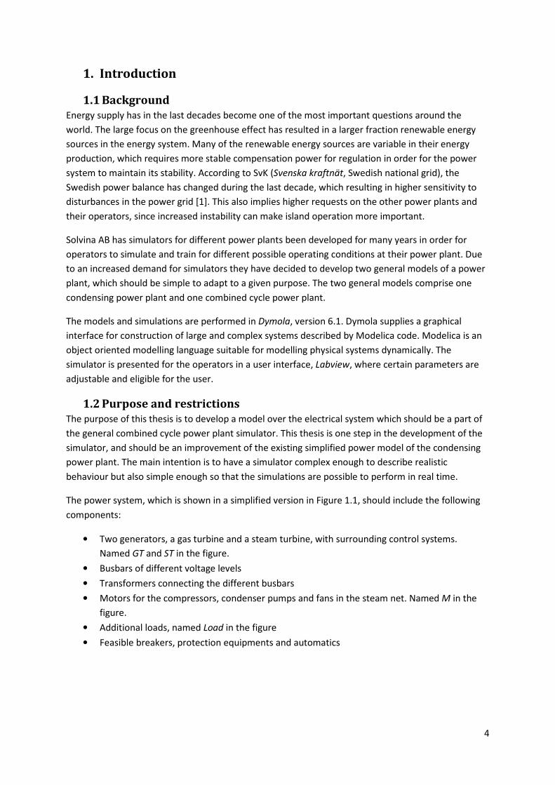
The power system, which is shown in a simplified version in Figure 1.1, should include the following
components:
• Two generators, a gas turbine and a steam turbine, with surrounding control systems.
Named GT and ST in the figure.
• Busbars of different voltage levels
• Transformers connecting the different busbars
• Motors for the compressors, condenser pumps and fans in the steam net. Named M in the
figure.
• Additional loads, named Load in the figure
• Feasible breakers, protection equipments and automatics

5
Figure 1.1: Overview of a general power system in a combined cycle power plant. In the
system there are two 130 kV busbars, where one gas turbine and one steam turbine
generator are connected, and two 6 kV busbars, where two motors and one arbitrary load are
connected, with four interconnecting transformers.
Further, the power system has to be able to simulate and fulfil the following:
• Simulation of cold start
• Normal load changes
• Trip of generator with a controlled behaviour of the system
• Controlled change-over to island operation and resynchronisation
The combined cycle power plant is composed of a gas turbine in combination with a waste heat
boiler which produces steam to a steam turbine consisting of a high pressure part and a low pressure
part, all mounted on the same shaft. This means that the power produced by the steam turbine is
limited by the steam flow, which is dependent on the amount of exhaust gases produced by the gas
turbine.
In order to perform simple adjustments of the general model to a specific power plant, this requires
rather high flexibility of the model. Further, the system should provide a realistic behaviour for
different operating conditions which requires high complexity and therefore quite high order of
some of the models. However, in order to run the simulations in at least real time speed, the
complexity of the model cannot be too high due to computational limits.
1.3 Limitations of the thesis
The system boundary of the project is drawn at the connection between the power plant and the
external power grid. However, in order to perform realistic simulations and to fulfil the requirement
about island operation a simplified model of the power grid has to be included.
Further, it is not within the limits of this thesis to unite the power system with the steam system in
the simulator. Instead, to verify the possible use of the power system it has to be capable of running
alone, although with connection to some simplified steam nets. Neither will any attention be paid to
the interface used for the simulator, LabView.

6
1.4 Outline of the thesis
In chapter 1 an introduction and overview of the thesis is presented. This aims to give the reader a
background to the purpose of the project.
Chapter 2 describes the methods used for achieving the project specifications and is also an outline
for the project work.
This is followed by a comprehensive theory part in chapter 3, which includes simulators for power
plants in general; the electric power system, both in general and the different components; a review
of island operation; and the modelling program. This part provides a broad background in all treated
areas of the thesis, and is the base for considerations performed in chapter 5 and 6.
In chapter 4 some simulators and power plants are presented, which are used as reference and
comparison. This gives background to some of the simplifications and assumptions made in the
modelling part.
The synthesised model is presented in chapter 5 followed by all the models of the different
components in chapter 6. The structure follows the structure given in chapter 3 for a simple
overview. Here all the assumptions, simplifications and approximations made during the modelling
are described for both the different components and the whole system. Chapter 5 also provides an
estimation of the complexity of the model and how well it can be performed in real time simulations.
The results of the simulations are presented in chapter 7, which includes validation of individual
components and the whole power system model. The validation results are discussed in chapter 8,
followed by conclusions and further research and possible improvements in chapter 9.

7
2. Method
2.1 Literature studies
Literature studies will be performed in order to obtain knowledge about the general structure of a
power system, its dynamics and the components included. There will also be access to older versions
of the power system which is going to be used as reference. Further, earlier developed power system
components can be obtained through the PowerSystem Library in Dymola [2].
Since the model is supposed to be integrated in the simulator later on, access to the other parts of
the simulator will also be needed.
2.2 Study visit
The simulator is supposed to be a general model over a combined cycle power plant; hence a real
system for comparison during the model construction does not exist. Therefore, in order to get
information about relevant components and control strategies during different operating conditions,
a study visit at the combined power and heating plant in Uppsala was performed. There exists also a
simulator over the power system in the pulp mill Södra Cell Mörrum that can be used for
comparison.
2.3 Modelling
There already exists a rather simple and inadequate model of the power system from the condensing
power plant simulator, from which a better and more complete model needs to be developed.
Each component in the power system will be analysed due to the requirements stated in Section 1.2
and will further be described in the theory part below. When considering electrical systems the “per
unit”-system is very useful, and therefore most of the models will be developed considering this.
The components and the system will continuously be controlled so that the requirements are
satisfactory fulfilled and that the behaviour is realistic.
From an earlier master thesis [2] a library (PowerSystem) of power system components has been
created and ready to use in new models. However, in order to fully understand the different
purposes of the models, and to be able to determine if the stated requirements are fulfilled, all the
components need to be evaluated. This is will be done both by simulations, where the behaviour is
controlled, and by studying the theory behind the models and how it is applied.
2.4 Simulations
In order to calculate and execute simulations differential algebraic equations (DAE) and ordinary
differential equations (ODE) have to be solved. The main difference between DAEs and ODEs, is that
a system of DAEs have dependent variables whose derivatives lack complete solution for all
components, which implies a non unique solution and the system cannot be solved explicit.
One of the requirements stated in Section 1.2 is that the simulations have to be performed in real
time in order to function as a simulator for training operators. This will be done in Dymola by
executing the models with fixed step integrators, like Runge-Kutta or Euler. However, this is a slow
and time-wasting way of dealing with the calculations, so to be able to perform more simulations in
shorter time all simulations will be performed with the variable step-size integrator DASSL,

8
developed especially for Dymola. DASSL is also the only integrator designed to solve DAEs, while the
others are designed to deal with ODEs, which means that the system has to be reduced in order to
perform real time simulations. The reduction occurs during the compilation.
In order to examine if the models can run in real time the fixed step integrator Rkfix4 will be used,
which is a Runge-Kutta method of order 4, also called the “classical Runge-Kutta method”.
Below a description of the different simulations that will be performed follows in order to verify the
specified model requirements.
2.4.1 Cold start of the system
This is done by connecting the external power grid to the power plant and starting the motors.
Thereafter starting the gas turbine generator, synchronise to the grid and increase the power
production. Starting the steam turbine generator after some time delay, synchronise to the grid and
increase the power production.
2.4.2 Load changes during normal operation
This is performed during normal operation by disconnecting a load from the system by using
breakers.
2.4.3 Trip of generator during normal operation
This is done during normal or island operation trigging the steam turbine generator to trip by
opening some breakers.
2.4.4 Island operation
This is performed by opening the net breaker out to the external power grid in order to simulate
island operation. The steam turbine will automatically shut down while the gas turbine will perform a
controllably change over to island operation. The control strategy will be voltage and
frequency/active power control.
2.4.5 Load change during island operation
This is performed during island operation by disconnecting a load from the system by using breakers.
2.4.6 Synchronisation of the power plant to the external power grid
By closing the breaker between the power plant and the external power grid, synchronisation of the
power plant to the external power grid can be simulated. The synchronisation system in the gas
turbine starts to adjust the gas turbine in order to fulfil the synchronisation requirements. When the
synchronisation is done the gas turbine generator changes its control strategy to active and reactive
power control, and the active power production will be increased.
9
3. Theory
3.1 Simulators for power plants
Simulators for power plants can be used for different purposes. Since different operation scenarios,
both common and rare, can be simulated, simulators can be very useful for training and education of
power plant operators. Further, the simulator can also be used for solving optimisation problems,
and is a cheaper alternative than using the real power plant.
However, this puts large requirements on the simulator. The main purpose for the simulator is not to
exactly resemble the power plant, but to behave like it. Since a real power plant is very complex, the
simulator has to be simplified, but without losing accuracy. It should still be possible to run the
simulator in real time, though limited by computational constraints.
Simulators can be over large power plants, or just a small part of the process.
3.2 Electric power system
3.2.1 Electric power systems in general
Electric power is an essential ingredient for many of the modern society’s fundamental functions.
There are many possible ways of power generation, like with renewable energy sources such as
hydro, wind and solar power, or with fossil fuels such as gas and coal.
Electric energy has the great advantage of being an energy carrier which is rather simple to convert
into other types of energy forms with reasonably low losses. Further, the transportation of electric
energy can be provided with transmission nets in a reliable way and with low losses, both long and
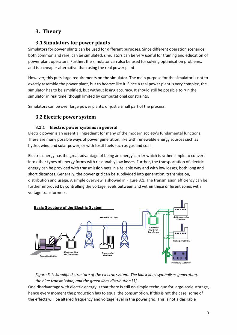
short distances. Generally, the power grid can be subdivided into generation, transmission,
distribution and usage. A simple overview is showed in Figure 3.1. The transmission efficiency can be
further improved by controlling the voltage levels between and within these different zones with
voltage transformers.
Figure 3.1: Simplified structure of the electric system. The black lines symbolises generation,
the blue transmission, and the green lines distribution [3].
One disadvantage with electric energy is that there is still no simple technique for large-scale storage,
hence every moment the production has to equal the consumption. If this is not the case, some of
the effects will be altered frequency and voltage level in the power grid. This is not a desirable

10
situation since some of the components in the power grid are rather sensitive to imbalance
conditions. The Transmission System Operators (TSO) are the ones responsible for keeping the power
system in balanced frequency conditions, which in Sweden is SvK. However, there are balance
providers, which are power producers with requirements on their production, which are also
responsible for balancing the power grid. In the end this puts a large control requirement on the
system operators to avoid imbalanced conditions.
The main components in a power grid are generators, motors, transformers, loads, transmission
nets, control devices, measurement and protection devices. These components are all going to be
described further in Section 3.2.2. The scope of this thesis is limited to the power grid of a combined
cycle power plant, and does, to some extent, not include the large transmission net.
3.2.1.1 Possible system simplifications
To model a power grid with all components and their dynamics included and to perform the
simulations in real time require large computation effort of the computers since the order of the
models can be very high. In order to perform the simulations within the right time limits and with
reasonable computational capacity certain approximations and simplifications have to be done.
There are many possibilities to reduce the order of the model [4]:
- By fundamental knowledge accumulate several coherent components to one equivalent
group
- Eliminate states that have small impact on the system
- By measurements create an equivalent circuit of the system
Due to the requirements of the power system model, all possible events are assumed to be
symmetrical, which implies that the three phase system can be reduced to a one phase system in the
model without losing any accuracy [5]. Further, if the system is supposed to have sinusoidal voltage
and currents, and the system frequency is nearly constant the jω-method can be applied, which
simplifies many of the calculations. The jω-method is a type of transform, and in circuit theory the j
implies a phase shift of 90 degrees. This method is applied during the modelling.
3.2.1.2 Stability and time-frame
Power system stability is defined as follows: “Power system stability is the ability of an electric power
system, for a given operating condition, to regain a state of operating equilibrium after being
subjected to a physical disturbance, with most system variables bounded so that practically the
entire system remains intact” [4]. The state of equilibrium is when [6]:
- The excitation voltages of the synchronous machines are constant
- All synchronous machines shafts rotate with the same electrical speed (i.e. synchronous
speed)
- The above described speed is constant
When a synchronous generator is subjected to a disturbance, the rotor of the generator is displaced
from its equilibrium point and the rotor will start to oscillate around the equilibrium. If the
disturbance is large, the displacement can be large enough to make the generator lose its
synchronism against the power grid, which results in large fluctuations in voltage, current and power.
When these occasions occur, protection equipment in the generator will disconnect the unstable

11
generator from the rest of the system. If the disturbance on the other hand is not large enough to
put the generator out of synchronism, smaller oscillations will transmit through the system.
Gradually the oscillations will decay and the system will regain its equilibrium [7].
Power system stability can be divided into different types of criteria: rotor angle stability; voltage
stability; frequency stability; mid-term and long-term stability. Rotor angle stability refers to the
capability of the system’s generators to remain in synchronism with each other after a disturbance
has occurred. Voltage stability describes the power systems ability to maintain voltages constant or
within reasonable limits during normal operation and after being subjected to a perturbation.
Likewise frequency stability refers to how well the power system maintains a stable, acceptable
frequency subsequent a severe system disorder causing a significant generation-load imbalance.
Mid-term and long-term stability consider problems associated with the power system dynamic after
severe disturbances. [4][7]
To further investigate the concept of stability it is favourably to categorise the concept into: (i) small-
signal stability and (ii) transient stability.
Small signal stability describes the ability of the system to remain stable (synchronous) when
exposed to small disturbances. Small disturbances frequently occur in a power system since the
generation not always equal the available loads, i.e. the production and consumption are not equal.
A small disturbance can also include switching of a capacitor or a load.
Transient stability describes the stability properties of the system when it is exposed to a severe
transient disturbance. The system response to such disturbance often results in large oscillations of
the rotor, stable or unstable. The disturbance is often large enough for the equilibrium reached
afterwards to differ from that before the occurrence of the disturbance. Real power systems are
often designed to handle various types of transient disturbances that may occur, like different kinds
of short circuits [7].
3.2.1.2.1 Time-frame
In order to perform an analytical evaluation of the stability properties of a system, another important
issue is the time-frame used in the analysis. Since the time constants vary significantly between the
different components of the system, it is often difficult to judge which time constant that dominates
or is the most important. This becomes really important for solutions in the time domain, since usage
of a too large time constant can fail to notice events of much shorter time-frame. Especially when
considering real time solutions, as will be the case in this thesis, where fixed step solvers are used. A
too small step size will significantly slow down the simulation, and a too large can miss out important
events.
3.2.2 Components in the power system
3.2.2.1 Generators
This thesis aims to model generators for gas and steam turbines. Therefore only high speed
synchronous generators with electromagnet rotors will be examined further on.
In order to magnetise an electromagnet rotor, the rotor windings are supplied with direct current,
the so called field current, by an external power source or by the generator itself. When the rotor
starts to rotate it exposes the stationary stator for a varying magnetic field, which induces an emf in
12
the stator windings. If the stator windings are connected to a balanced three phase system, then the
appeared magnetic field will rotate with the same frequency as that system, which in Sweden has the
nominal value of 50 Hz. In order to produce an even torque the magnetic field of the rotor and the
magnetic field of the stator must rotate synchronously, as the name also indicates, which is why this
speed is called the synchronous speed. Equation 3.1 shows the relation between the
synchronous speed [rpm], the power system frequency [Hz] and the number of pole pairs in
the generator. However, when a load is applied to the stator the magnetic axis of the rotor will be
slightly ahead of the stator magnetic axis in order to convert the torque applied on the rotor into
useful electricity in the stator windings.
Equation 3.1
Synchronous generators have high efficiency and possibility of producing active and reactive power
independently. The latter entail the synchronous machines to be used as voltage regulation
equipment and for correcting the power factor in the system, although this is outside the limits of
this thesis and will not be considered further on.
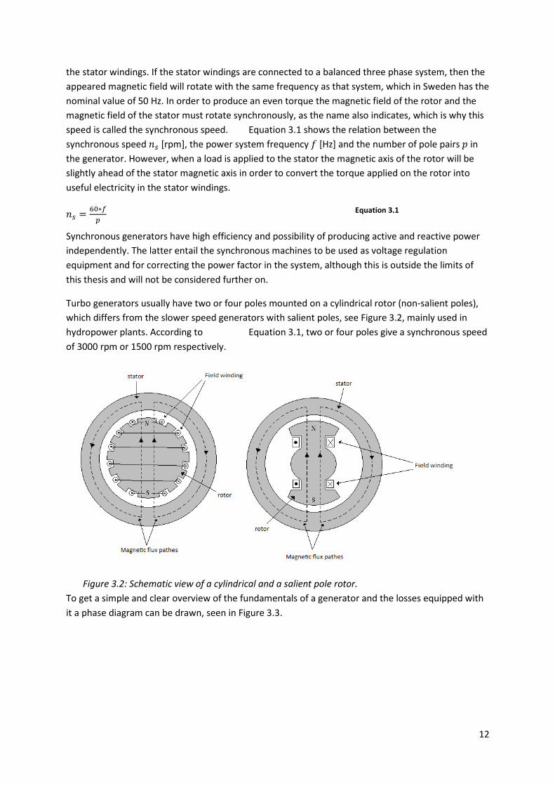
Turbo generators usually have two or four poles mounted on a cylindrical rotor (non-salient poles),
which differs from the slower speed generators with salient poles, see Figure 3.2, mainly used in
hydropower plants. According to Equation 3.1, two or four poles give a synchronous speed
of 3000 rpm or 1500 rpm respectively.
Figure 3.2: Schematic view of a cylindrical and a salient pole rotor.
To get a simple and clear overview of the fundamentals of a generator and the losses equipped with
it a phase diagram can be drawn, seen in Figure 3.3.
13
IVt
I*Ra
jI*Xl
jI*Xm
Ef
Eδ
δrφ
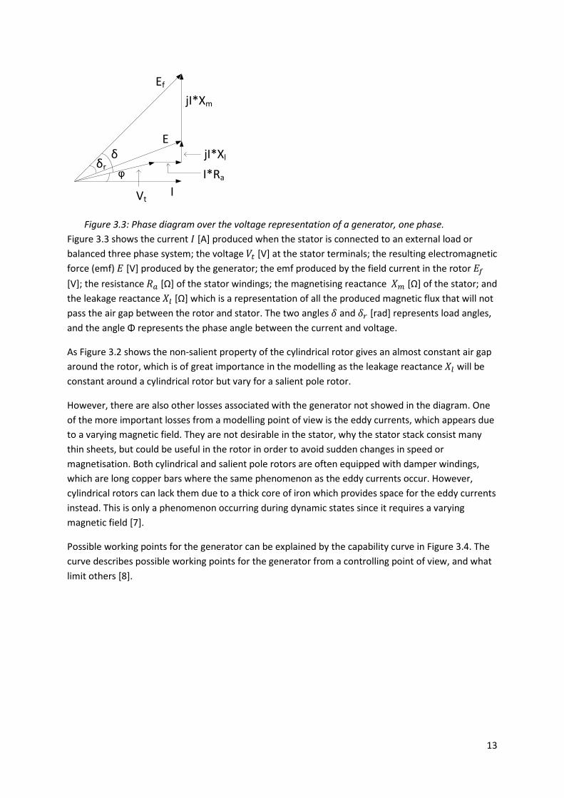
Figure 3.3: Phase diagram over the voltage representation of a generator, one phase.
Figure 3.3 shows the current [A] produced when the stator is connected to an external load or
balanced three phase system; the voltage [V] at the stator terminals; the resulting electromagnetic
force (emf) [V] produced by the generator; the emf produced by the field current in the rotor
[V]; the resistance [Ω] of the stator windings; the magnetising reactance [Ω] of the stator; and
the leakage reactance [Ω] which is a representation of all the produced magnetic flux that will not
pass the air gap between the rotor and stator. The two angles and [rad] represents load angles,
and the angle Φ represents the phase angle between the current and voltage.
As Figure 3.2 shows the non-salient property of the cylindrical rotor gives an almost constant air gap
around the rotor, which is of great importance in the modelling as the leakage reactance will be
constant around a cylindrical rotor but vary for a salient pole rotor.
However, there are also other losses associated with the generator not showed in the diagram. One
of the more important losses from a modelling point of view is the eddy currents, which appears due
to a varying magnetic field. They are not desirable in the stator, why the stator stack consist many
thin sheets, but could be useful in the rotor in order to avoid sudden changes in speed or
magnetisation. Both cylindrical and salient pole rotors are often equipped with damper windings,
which are long copper bars where the same phenomenon as the eddy currents occur. However,
cylindrical rotors can lack them due to a thick core of iron which provides space for the eddy currents
instead. This is only a phenomenon occurring during dynamic states since it requires a varying
magnetic field [7].
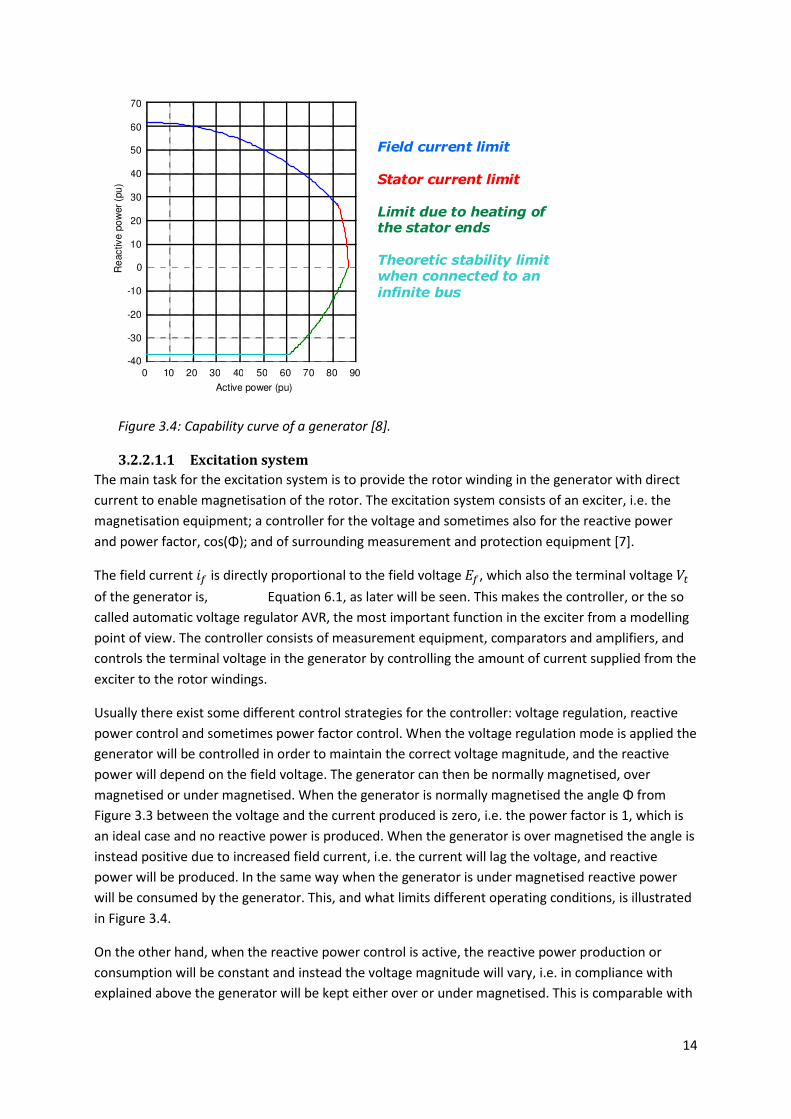
Possible working points for the generator can be explained by the capability curve in Figure 3.4. The
curve describes possible working points for the generator from a controlling point of view, and what
limit others [8].
14
0 10 20 30 40 50 60 70 80 90 -40
-30
-20
-10
0
10
20
30
40
50
60
70
Re
activ
e p
ow
er
(pu
)
Active power (pu)
Field current limit
Stator current limit
Limit due to heating of the stator ends
Theoretic stability limit when connected to an
infinite bus
Figure 3.4: Capability curve of a generator [8].
3.2.2.1.1 Excitation system
The main task for the excitation system is to provide the rotor winding in the generator with direct
current to enable magnetisation of the rotor. The excitation system consists of an exciter, i.e. the
magnetisation equipment; a controller for the voltage and sometimes also for the reactive power
and power factor, cos(Φ); and of surrounding measurement and protection equipment [7].
The field current is directly proportional to the field voltage , which also the terminal voltage
of the generator is, Equation 6.1, as later will be seen. This makes the controller, or the so
called automatic voltage regulator AVR, the most important function in the exciter from a modelling
point of view. The controller consists of measurement equipment, comparators and amplifiers, and
controls the terminal voltage in the generator by controlling the amount of current supplied from the
exciter to the rotor windings.
Usually there exist some different control strategies for the controller: voltage regulation, reactive
power control and sometimes power factor control. When the voltage regulation mode is applied the
generator will be controlled in order to maintain the correct voltage magnitude, and the reactive
power will depend on the field voltage. The generator can then be normally magnetised, over
magnetised or under magnetised. When the generator is normally magnetised the angle Φ from
Figure 3.3 between the voltage and the current produced is zero, i.e. the power factor is 1, which is
an ideal case and no reactive power is produced. When the generator is over magnetised the angle is
instead positive due to increased field current, i.e. the current will lag the voltage, and reactive
power will be produced. In the same way when the generator is under magnetised reactive power
will be consumed by the generator. This, and what limits different operating conditions, is illustrated
in Figure 3.4.
On the other hand, when the reactive power control is active, the reactive power production or
consumption will be constant and instead the voltage magnitude will vary, i.e. in compliance with
explained above the generator will be kept either over or under magnetised. This is comparable with

15
the power factor regulation where it is the relation between the active and reactive power produced
which is kept constant.
In many excitation systems the voltage regulation is always active while the reactive power
regulation is exterior with a slower control loop and applicable if desired.
3.2.2.1.2 Turbine governor
The primary task for the turbine governor is to stabilise frequency variations in the power system by
instant control of the produced active power, but at start and stop to accelerate and decelerate the
generator speed by controlling the power produced by the turbine. In this case it is performed by
adjusting the valve of gas or steam flow to the turbines [9].
Turbine governors have something called power frequency characteristics, which is defined as
follows:
∆
∆ Equation 3.2
where ∆ is the change in active power and ∆ the change in frequency. This implies that the power
frequency characteristic is a measure of for example how much more active power has to be
produced in order to maintain the right system frequency after a frequency drop. It is also a
specification for the stiffness in a power system. This property becomes important when there are
two or several governors controlling the same load in a system, since the change they imply depends
on their own power frequency characteristic [10] [9].
The governor can have different control strategies, where frequency control, frequency/active power
controlling, and active power controlling are most common.
3.2.2.1.3 Synchronisation controller
In order to synchronise two alternating current systems with each other there are five conditions
that have to be fulfilled:
- Same voltage level in the two systems
- Same frequency
- Same phase angle
- Same phase sequence
- Same waveform
The waveform and the phase sequence are decided by the outline of the generator, which is
supposed to be the same for the generators in this power system model. However, the
synchronisation system has to provide the fulfilling of the remaining conditions.
The synchronisation can usually be performed manually or automatically, but in this thesis only
automatic synchronisation will be possible. During synchronisation of a generator to a power system
the required conditions are obtained by letting the excitation system adjust the voltage level by
controlling the rotor field current, and the turbine governor adjust the frequency by controlling the
power supply from the turbine.

16
3.2.2.2 Transformers
Power transformers are necessary in order to unite the parts of different voltage level in the system.
In addition to this, transformers are often used for voltage regulation and control of the reactive
power flow by using tap changers in order to change the turn ratio and hence the voltage level on
the secondary side [11]. Other types of transformers are the current transformer and the voltage
transformer used in measurement devices, which are not interesting for this thesis.
The most common power transformers, which for simplicity from now on will be called only
transformers, are the ordinary single-phase with two coils, also called double-wound transformers.
Other types could be made of one coil and of several coils. For a three-phase system the most
common is to use three single-phase transformers together in one set. However, it is also possible to
have one common core for the three windings, which is also valid for other poly-phase systems. In
the three phase system the Y and delta connections are the most regular ones [11].
Independent of where or for what purpose the transformer is used, the basic working principle is the
same. The principle is built around electromagnetism, i.e. that an electric current produces a
magnetic field, and electromagnetic induction, which states that a changing magnetic field within a
coil produces a voltage across the coil. Most transformers are basically made of a core with high
magnetic permeability, like iron, with two coils wrapped around each side, named primary and
secondary side, see Figure 3.5. By connecting the primary side to an alternating voltage source
producing an alternating current, represented by and respectively in the figure, a changing
magnetic flux appears in the core, represented by the crosshatched line. Due to electromagnetic
induction, the changing magnetic flux induces a voltage in the coil of the secondary side. and
in the figure symbolises the number of turns for the primary and secondary coils respectively [11].
Figure 3.5: Diagram over a single- phase ideal transformer.
The concept of an ideal transformer contains no resistive losses associated with iron or copper, no
leakage reactances associated with magnetic losses, and the core is regarded to have infinite
magnetic permeability and infinite electric resistivity. The following relation can then be obtained:
!
"
#!
#"
$!
$" Equation 3.3
which gives that the transformation of voltages in an ideal transformer is proportional to the turning
ratio . For the currents the following relation holds:

17
%!
%"
$"
$!
& Equation 3.4
which gives inversely proportionally of the current to the turning ratio [11].
However, for practical uses we need more than the ideal model of a transformer. In reality there are
losses in the transformer need to be taken into consideration to obtain a more realistic model. These
losses are associated with ohmic resistance, magnetic resistance and magnetic leakage flux. The
ohmic resistances are associated with the copper in the windings, and , and with the iron in the
core, which is due to magnetic hysteresis and can be approximated with a shunt resistance '. The
magnetic resistance is due to a finite permeability of the iron core, hence a reluctance which is not
zero, and therefore some current is required for magnetise the core. This can be symbolised with a
shunt reactance . Some of the magnetisation flux will not pass both the primary and secondary
side, and hence not conduce to induction. This can be represented with leakage reactances ( and (
which are usually much smaller than . Figure 3.6 below shows the equivalent circuit of the non-
ideal transformer with all components just described [11].
Figure 3.6: Equivalent circuit of a non-ideal transformer.
The parameters can be determined practically through open-circuit and short-circuit tests. An open-
circuit test provides the values of ' and , while (, (, ) and )are given by the short-circuit test.
If these tests are unavailable a simplified model can be obtained by neglecting the iron and
magnetising losses, hence approximate the no-load current to zero [11].
3.2.2.2.1 Tap changer
As mentioned in Section 3.2.2.2, transformers can be used for voltage regulation by using tap
changers in order to control the voltage on the secondary side, which is also the most common way
to perform voltage regulation in Sweden. To use capacitor banks is also relatively common in larger
distribution systems [12]. In the scope of this thesis the tap changer will be considered, as will shunt
capacitors in Section 3.2.2.5.3. Another advantage with tap changers is that the voltage level in the
power system can be kept constant regardless, at least to some extent, of load variation [4]. Further,
by changing the voltage levels the reactive power flow can be controlled at different busbars and
subsystems, hence the active and reactive power losses can be controlled [6].
The tap changer can be connected either to the high voltage or the low voltage side of the
transformer. In large transformers, the volt per turn is quite high and to change one turn on the low
voltage side results in a large percentage change in the voltage. Further, the load current on the low

18
voltage side can be very high, and thus the taps would better be connected to the high voltage
(primary) side. A principle scheme of the tap changer is showed in Figure 3.7.
Figure 3.7: Principle scheme of a transformer with tap changer
There are two types of tap changers: on-load and off-load (or de-energised). The off-load tap changer
changes the tap positions via a switch when the transformer is completely de-energised, and then
reconnected to the circuit. This provides a rather simple construction and hence a relatively low cost.
However, this situation is not desirable for the aim of this thesis where a more automatic control is
preferable [13].
The on-load tap changer (OLTC) changes the tapping of the transformer when the transformer is still
in operation and energised, and may be controlled manually or automatically. According to [12] the
control of the OLTC is usually discrete valued and based on a local voltage measurement. Usually the
tap ratio change is around ±10-15 % and performed in steps of 0.6-2.5 %. The tap changing is
associated with some time constants, including mechanical time delay (usually 1-5 s) and actual tap
operation time (around 0.1-0.2 s). The deadband relates to the tolerance for long-term voltage
deviations, and the time delay usually contributes for noise rejection [12]. According to [2] the
deadband can be described with the following relations:
*+ * ,1 .∆/
0 Equation 3.5
*%& * ,1 ∆/
0 Equation 3.6
where * is set point and ∆* the degree of sensitivity, given as percentage of *. When the voltage
deviation reaches beyond the dead zone the time delay described above will act before the tap ratio
is changed. According to [12] the time delay is typically around 30-120 s and the dead zone slightly
smaller than two tap steps.
3.2.2.3 Loads
The term load in this context comprises all components in a power system that consumes active or
reactive power, like motors but also transformers. Since the stability of a power system is highly
dependent on the balance between produced and consumed power, the load characteristics are very
important. There are normally a large amount of components consuming power in a power system,

19
like motors, lamps, compressors and so on, and the exact quantity may be complicated to estimate.
On the other hand if the exact load composition is known, to symbolise each component may just be
impractical since the large amount only makes the system more complicated [7].
Normally, the most complicated models in the power system are the synchronous machines and
their transient behaviour usually has to be considered in order to emulate a realistic behaviour.
Other components in the power system, like transmission lines and transformers, do not usually
influence the electromagnetically phenomenon significantly, and a detailed representation is seldom
justified [6]. Therefore, certain simplifications and assumptions have to be made in order to create a
sufficient load representation.
The models can be divided into frequency dependent models and voltage dependent models. For
simplification it may also be beneficial to divide the voltage dependent models into two categories:
static models and dynamic models. The total load can either be represented by one of these
individual models, or as a combination of them [7].
3.2.2.3.1 Frequency dependent load models
When considering merely resistive loads like lightning installations or heaters, the power
consumption is frequency independent. This is not true for motor loads, like pumps and fans, where
the power consumption varies with the frequency due to the torque/speed characteristic. As the
frequency in the system increases, the power consumption by the motor increases and hence the
effect of the frequency raise is damped. Therefore, this type of load has an inherent stabilising effect
on the system [7] [11].
Since motors are very important in the power system, their properties will be further emphasised in
Section 3.2.2.4.
3.2.2.3.2 Static load models
The static model aims to describe static components in the power system, but is also used as an
approximation for dynamic components [7]. Generally when considering normal operating conditions
the voltage and frequency dependency is neglected and the loads are regarded as constant active
and reactive power consumers [5].
An alternative load model for representing the voltage dependency (neglecting the frequency
dependence), namely the polynomial model, is seen in Equation 3.7 and Equation 3.8 [7].
12 . 2 . 34 Equation 3.7
5 5162 . 62 . 634 Equation 3.8
A common name for the polynomial model is ZIP, since the components represent constant
impedance (Z), constant current (I), and constant power (P) respectively. The parameters to 3,
and 6 to 63are coefficients defining the amount of each subcomponent required to describe the
original model [7].
Constant impedance (Z)
Loads represented by a constant impedance model have power consumption proportional to the
voltage magnitude squared, i.e. the first components in Equation 3.7 and Equation 3.8. Practically
this can be an approximation for lightning installations and different heaters [5].

20
Constant current (I)
Loads with constant current property represent models where the power consumption is linearly
proportional to the voltage magnitude.
Constant power (P)
Constant power consumption characteristic regard voltage invariant loads, i.e. this concept represent
loads or composite loads with stiff voltage characteristic. Composite loads may also consist of a
voltage dependent load together with a transformer equipped with tap changer and seen from the
power grid these together automatically receives constant voltage [5].
3.2.2.3.3 Dynamic load models
Normally, when composite loads are subjected to changes in frequency or voltage which are of
modest amplitude the response is fast and the steady state reaches quickly. These cases justify usage
of static load models. However, there are cases were the slower dynamic responses of the load may
affect the electromagnetic phenomenon significantly, like studying the longer time-frame of voltage
stability and long-term stability. One important component which needs the dynamic model
representation is the motor, which is discussed further in Section 3.2.2.4. The main difference
between the static and dynamic representation is the influence of not only the present but also the
former voltage and frequency values in the dynamic model [6][7].
The following examples are also components which require dynamic models in order to perform an
accurate stability analysis of the system [7]:
• Protective relays: like overcurrent relays which are used in order to protect for example
industrial motors. Due to the overcurrent that occurs when the voltage drops, these usually
drop open when the voltage has been between 0.55-0.75 pu during a few cycles. More about
this in Section 3.2.2.6.
• Tap changers and voltage-controlled capacitor banks: in many cases these devices are
included in the load models directly. Their function is to restore the voltage level of the load
after being subjected to a disturbance. However, their control action is noticeable first after 1
minute, and the voltage is restored within 2-3 minutes.
3.2.2.4 Motors
The most common used motor in industrial purposes is the induction motor, due to its low cost and
reliability. The synchronous motors are mainly used as power compensators in order to adjust the
power factor in the power grid or at large pump plants, and therefore beyond the scope of this
thesis.
In a combined cycle power plant there are many different motors involved in the process, for both
pumps and fans. Nevertheless they can be subdivided into: constant speed controlled motors, and
variable speed controlled motors. There is also a difference between those motors that are directly
started and those with only a starting resistance and the power is increased gradually, mainly due to
the physical size difference, hence the starting torques.
In contrast to synchronous machines, the induction machine carries alternating currents in both the
stator and the rotor windings. The motor of relevance to this project, the rotor has internally short-
circuited windings, also called squirrel-cage, not supplied with power. During the starting sequence
the motor experiences a large current, which occurs since the motor to trying to create a magnetic

21
field in the rotor, and is a severe problem for larger machines. It is not unusual for the starting
current to be six times larger than the normal load current [11].
The basic working principle of an induction machine is as follows. By connecting the stator windings
to a balanced three phase power system a rotating magnetic field will appear in the stator. This
magnetic field will induce currents in the rotor windings and hence a magnetic field. The reaction
between these fields produces a torque which accelerates the rotor in the stator fields’ direction of
rotation. The small difference that occurs is called slip which is negligible at no load; hence no torque
is produced then since no current is induced in the rotor windings. The slip is defined in
Equation 3.9, where ωs is the synchronous speed and ωr the rotor speed. The slip
increases, i.e. the rotor speed decreases, when a load is applied in order to produce the required
torque. These properties make the induction machine, unlike the synchronous machine, inherently
self-starting [7][11].
7 89:8;
89 Equation 3.9
The equivalent circuit for an induction motor, one phase, is showed in Figure 3.8, where Rs is the
stator winding resistance, xs the stator leakage reactance, Rr the rotor resistance referred to the
stator and dependent on the slip s, xr the rotor leakage reactance referred to the stator, Rc the core
loss, and Xm the magnetising reactance [11]. A common approximation is to neglect the core loss
component Rc, since this loss is usually relatively small.
Figure 3.8: Equivalent circuit for an induction motor.
3.2.2.5 Transmission net, breakers and shunt capacitors
3.2.2.5.1 Transmission line
The outline of the transmission net depends on several variables. The power can be transmitted by
overhead power lines or underground power lines, where overhead power lines are most common
and usually also cheapest. Further, the voltage used for transmission is determined by the distance
and power transmitted.
The general equivalent circuit (one phase) for a transmission line is showed in Figure 3.9, where Z
represents the series impedance and Y the shunt admittance, which are assumed to be uniformly
distributed along the transmission line [7].

22
Figure 3.9: Equivalent π-circuit of a transmission line.
Transmission lines are not within the scope of this thesis, but are present in the model to represent
the external power grid transmission lines if desired. For the moment it does not add any dynamic to
the model since the external power grid is represented by an infinite bus. Cables within the power
plant are too short to provide significant voltage drops, and are therefore neglected.
3.2.2.5.2 Breakers
There are several different types of breakers appearing in the power system, depending on the
intended use and the voltage level. The most common ones are showed in Table 3.1, and how they
are applied in this thesis [14].
Breaker Switching capability Field of application Comment
Circuit-breaker Load currents, short-circuit currents
Most common in the power system
Further described in Section 3.2.2.6
Load-break switch Load currents
Disconnecting switch
Under no-load conditions
For completely de-energised circuit
No application in this thesis
Earthing switch For earthing equipment
Can be used for simulating earth faults
Fuse Low and middle voltage systems
Too narrow field of application for this thesis
Table 3.1: The most common types of breakers appearing in the power system.
3.2.2.5.3 Shunt capacitors
Shunt capacitors and series capacitors are examples of compensation components in the power
system. In the Swedish power system it is very common to have large capacitor banks or
synchronous compensators which is synchronous machines running without mechanical load,
although the latter one is not as common any more. There are also other common compensation
components like shunt reactors, but in this thesis only static shunt capacitors will be concerned.
Capacitors produce reactive power and are used for lagging power-factor circuits since they
themselves have a leading power-factor. As described earlier, the amount of reactive power and the
voltage level in a power system is strongly related; hence by producing reactive power the capacitor
can maintain the right voltage magnitude. They are usually applied in low or medium voltage

23
systems. Where there are a lot of induction machines which require a large amount of reactive
power, like in many industries, there are usually local compensation with capacitor banks in order to
avoid affecting the power-factor too much [10][14][8].
The reactive power production from a shunt capacitor is proportional to the voltage squared, which
means that if the voltage decreases the reactive power production will also decrease, which is an
unfortunate property since it is needed most then. The shunt capacitors can either be constantly
connected to the system, or automatically or manually connected and disconnected to the system
depending on the voltage level. When they are automatically connected and disconnected there is
usually a deadband zone in order to avoid too much fluctuation [10][8].
3.2.2.6 Protection systems
During its lifetime, a component in a power system is generally assumed to withstand the anticipated
loads during normal and emergency operating conditions and are hence designed and constructed
due to this constraint. However, it is neither economically sustainable nor technically realistic to
endorse the design to hold for all possible disturbances or loads. Therefore the need for protection
systems becomes necessary in order to limit the fault effects.
The task for the protection system is to decide when the operating condition is no longer normal and
then as soon as possible successfully isolate the damaged or endangered component. However, it
should be remembered that it is not in the responsibility of the protection system to avoid these
faults or disturbances. The allocation of the protective systems is in general made in order for each
component to be completely disconnected from the rest of the system. There are many abnormal
operating conditions that should be taken into account, where short circuit is seen as the most
important one [14][15].
There are a wide range of different types of protection systems appearing in the power system, why
only the most important will be considered in this thesis. There are also protection systems providing
protection for events not likely to occur or possible to simulate for this type of model, why they will
be neglected. An individual description of them follows beneath.
3.2.2.6.1 Current protection
Overcurrents can occur in a power system due to short-circuits or overload and can cause severe
damage on different components in the power system. Usually overcurrent protection is applied to
transmission lines, transformers, motors and generators [14].
3.2.2.6.2 Voltage protection
It is important to keep the right voltage level in a power system in order to maintain the best
performance. Overvoltages can be divided into two different types: external and internal. As the
names suggest, the difference is due to where the cause of the overvoltage is located. External
overvoltages are mainly due to lightning, whilst internal overvoltages can occur due to load-
shedding, switching operations, and resonance phenomena. Voltage decrease or dip is normally due
to short-circuits and motor start-ups, whereas a change in the neutral voltage is typically due to
earth-fault. Overvoltage protection and earth-fault protection are usually used for transmission lines,
transformers and generators, while the undervoltage protection is usually applied on motors and
generators [14][16].
24
3.2.2.6.3 Frequency protection
This type of protection system is not mentioned above, mainly because it is usually embedded in
other parts of the system. However, since its function is essential for the performance of the power
system it has to be further described.
As mentioned before, the frequency in a power system is very important, especially for frequency
dependent motors and transformers, due to possibly large magnetisation currents. A change in
frequency occur when a change in load or short-circuits appears. Under-frequency is due to increase
of load, and over-frequency is related to loss of load. The protection for frequency changes is
generally seen as a general task of the system protection, since the change is strongly related to the
balance between produced and consumed power in the system. Normally protection is also provided
for generators [14].
3.2.2.6.4 Magnetisation protection
The magnetisation protection is not mentioned as one of the more common protection systems, but
nevertheless important in this context. This protection device is partly like the voltage and frequency
protection above, and is used to protect the transformer from overmagnetisation, which could be a
likely event to occur in this power system model.
3.2.2.6.5 Reversed power protection
The main task for the reversed power protection is to assure that the direction of the power flow is
not reversed, which is especially important for generators in order to keep their operating point
within the limits as described in Figure 3.4. A change in direction of the power flow can occur due to
short-circuit [14].
3.3 Island operation
Swedish national grid (Svenska kraftnät, SvK) is a state utility that has the overall responsibility for
the Swedish power grid, which implies being the system operator. The main responsibility for the
system operator is to maintain the electricity system in balance, which is performed by commanding
the electricity producers to increase or decrease their production, and ensure the installations to be
operated in a reliable way. During situations of electricity shortage they are also responsible for the
priority plan [17].
If there is a shortage of electricity and the priority plan has to be complied certain regional or local
parts can be disconnected from the main power grid. This can also happen automatically during
disturbances on the power grid which makes some power producing units to disconnect, and the
state that appears is called island operation. In an island operation situation the local or regional
disconnected area has to maintain the stability and balance between produced and consumed power
itself, which can be quite difficult in small areas.
The situation described above is beyond the limits of this thesis. However, in this thesis the term
island operation concerns only a single power plant, also called house load operation. SvK has stated
this event for large power plants like nuclear power plants and combined cycle power plants.
According to [1] a successful island operation for a power plant is when the change-over happens
controllable and the power production is adjusted to only concern the internal consumption. If such
state appears the power plant can easily be reconnected to the main power grid and increase the
power production immediately, and hence the power grid can quickly be restored. This is a situation
25
to prefer instead of an unsuccessful change-over which causes the power plant to shut down; hence
a longer time for restoration. In most countries island operation is the common state during a power
loss on the main power grid [1].
As stated in Section 1.2, one of the requirements for this model is to perform a successful change-
over to island operation. In order to perform this some control strategies has to be considered,
further described in Section 3.4.
3.4 Control strategies
The control strategies for this model can be divided into four different overall control modes:
• Synchronisation of generator: the control is performed by the generator controllers. In order
to fulfil the synchronisation conditions described in Section 3.2.2.1.3 the generator has to be
in voltage regulation and frequency control mode. Since the steam flow depends on the
power produced by the gas turbine, the steam turbine generator cannot start if the gas
turbine is not running.
• Normal operation: the excitation system starts to control the reactive power and the turbine
governor to control the active power. Thus the active and reactive power produced can be
adjusted.
• Island operation: the generators have to return to voltage and frequency control in order for
the power plant to maintain stable and balanced. However, when two generators are trying
to imply their frequency on one weak system, either one of them or both has to have statics.
This means that the turbine governor will also consider the active power in the system.
• Synchronisation of power plant to grid after island operation: in order to fulfil the
synchronisation conditions described in Section 3.2.2.1.3 the generators has to be in voltage
regulation and frequency control mode. Only the deciding generator, usually the strongest,
has to be adjusted since the generators are connected.
3.5 Modelling program
Performing a transient stability analysis requires solving a system of non-linear differential equations.
The most practical method to achieve this is for the moment by using numerical integration
techniques in time domain simulations [7]. The modelling tool used in this project is Dymola, version
6.1. Dymola is a program package using the program language Modelica.
3.5.1 Modelica
Modelica is an object-oriented modelling language produced in order to simplify modelling of large
and complex physical systems. It is especially made for modelling in more than one domain, e.g. for
systems containing mechanical, electrical, hydraulically, and thermal subsystems. To be able to
describe physical phenomenon with models, Modelica uses equations like ordinary differential
equations (ODE), algebraic equations and discrete equations from which large differential algebraic
equation systems (DAE) are created and solved numerically. The main purpose is to create balanced
models where the number of unknowns equals the number of stated equations [18].
Since Modelica is an object-oriented modelling language there are many similarities with ordinary
object-oriented program languages like Java and C++. However, there are two major differences.
First of all, as mentioned before, Modelica is not a program language but a modelling language,
which implies certain differences in the simulation process and the translation of the classes into

26
objects. The second difference concerns causality, where Modelica unlike many other program
languages, does not translate the equality sign in an equation as an assignment, but instead as a
mathematical property. Due to this it is possible to have several unknowns on both sides of the
equality sign, which simplifies the managing of physical systems. Another advantage is also that the
equations do not have to be in the same order as they will be solved [18].
Modelica has a property which enables usage of earlier created models in new models without the
requirement of reproduce all the properties of the old model. Furthermore, the models are built in a
hierarchical way which increases the simplicity and stocktaking during the construction process [18].
3.5.2 Dymola
As mentioned before is Dymola, or Dynamic Modelling Laboratory, a program package using
Modelica as a modelling language. Dymola supplies a graphical interface for construction of models
where a combination of graphic construction and programming with Modelica code is used.
However, it is not possible to change things in the models during simulations with this interface,
which is why the simulator is using a different interface, Labview. Further, there are ready-made
basic data types and models, and also a possibility for producing own libraries with self-made
models.
Further, Dymola also provide simulation possibilities, where the simulations can be performed with
fixed step or variable step-size integrators depending on the purpose. As mentioned in Section 2.4, in
order to perform real time simulations fixed step integrators like Runge-Kutta is preferable, while
nonlinear DAE better be solved with variable step-size integrators like DASSL.
In order to perform simulations, Dymola translates the Modelica code into C++ code since it speeds
up the simulations. The Modelica specification never define how a model should be simulated,
instead it defines a set of equations that should be satisfied as well as possible by the simulation
result. However, many of the models are higher order index systems, and in order to simulate them
in an appropriate way a symbolic index reduction has to be performed. This is done by differentiating
the equations and selecting appropriate variables as states. In this way the resulting system of
equations can be transformed into the easier solvable state space form [18].
When dealing with fixed step integrators the selection of step-size is very important from a stable
and converging solution point of view. The essential condition is to have a step-size shorter than the
shortest significant time constant in the system as described in Section 3.2.1.2.1. In the setup of the
simulation a choice of tolerance has to be made. This is related to the calculated local error for each
component at every time as follows:
|=>?@= ))>)| B )=@C C>=)@? |(%| .
@D7>=EC C>=)@?
Equation 3.10
where (% is the state vector for the simulated problem. In Dymola the relative and absolute tolerance
is equal, which may be a problem when dealing with signals of significant difference. It is therefore
an advantage to scale the signals to be in the same order of magnitude, which in this case is simplest
to obtain by using the per unit system.

27
4. Reference power plants
4.1 The combined power and heating plant in Uppsala
At the combined power and heating plant in Uppsala, owned by Vattenfall AB Heat Nordic, electricity
and district heating is produced to the city of Uppsala by burning peat and wood chip. The full
capacity of the plant is 245 MW district heating and 120 MW electricity where the production is
regulated according to the heating demand. District heat is also provided by the nearby plants of AFA
(waste incineration) and Bolandsverket, which produces both heat and steam. Earlier this year (2010)
a new steam turbine was installed at AFA for electricity production [19].
The old steam turbine of the combined power and heating plant consists of one high pressure
turbine, one middle pressure turbine and one two pole turbo generator. The magnetisation of the
rotor is provided by a brushless rotating exciter, which implies there is no need for an external power
source for supplying the field current. In order to synchronise the generator the turbine is
accelerated manually to the right rotational speed, by when the magnetisation of the rotor is started.
The synchronisation to the external power grid is provided automatically.
The power plant is constructed to enable island operation and autarky, and Vattenfall is also
bounded by contract to help out in the start-up of the power grid in Uppsala if being subjected to a
blackout. The obtainable emergency power is through a gas turbine. However, neither of these
events has yet been performed in reality according to [20].
The power plant is mainly active during the cold period of the year. This is due to the controlling
scheme mentioned in the beginning, i.e. that the production is regulated according to the heating
demand and not for maximising the electricity production, which can be the case in other power
plants.
The plant has four large transformers, three of them equipped with tap changers. There is also
another transformer providing Bolandsverket with electricity from the external power grid. The tap
changing usually happen automatically, but there is a possibility for manual performance. It exist
double sets of busbars for high, middle and a higher low-voltage level; and a single for a lower low-
voltage level. All the large power consumers within the plant, like fans for air and flue gas and pumps
for condensate and district heating water, are all connected to the middle voltage level busbar. There
is also a turbine driven pump for feed water possible to start up by using electricity. Of these loads it
is only the pump for the district heating water which is speed controlled, while all the others run with
constant speed. The pumps are direct started while the fans are started only with a starting
resistance and then the power is increased gradually due to their large physical size [20].
4.2 Södra Cell Mörrum
Södra Cell Mörrum is a pulp mill in the south of Sweden producing pulp for the paper mills in Europe,
and electricity and district heating for the city of Karlshamn nearby. The plant has three steam
turbines and three transformers with tap changers connected to each generator [21].
Solvina AB has performed several projects at Södra Cell Mörrum, and therefore a model and a
simulator over the power system exists in Dymola. This simulator has also been used during a course
about electric power dynamics internally at Solvina AB [8].

28
During normal operation it is usually only active power being produced to the external grid [21]. The
simulator is supposed to be a slightly simplified version of the real plant but still realistic, and below
follows a description of the components included.
The simulator has three synchronous generators, each equipped with a turbine regulator which has
six different control modes: frequency control, frequency/active power control, active power control,
back pressure control, steam flow control and boiler pressure control. When the pulp mill is past over
to island mode the turbine regulator automatically change over to frequency/active power control
with statics for two of the generators. The excitation system can either control the voltage or the
reactive power, where the voltage regulation is used during island operation [8].
Further, the tap changers connected to each transformer has a deadband and a time delay after
crossing the deadband area in order to avoid too much fluctuation when changing the turning ration
of the transformer [8].
The loads in the model are mainly induction machines, but there are also some fixed loads and an
impedance load which represents additional loads in the power plant. To supply the system with the
right amount of reactive power there are also some shunt capacitors connected. Even though the
original pulp mill is equipped with several protection systems, the simulator is slightly simplified and
has only protection in the generators for over and under frequency [8].

29
5. Synthesised model of the power system
5.1 Overview of the model
As mentioned in the purpose of this thesis, the model of the combined cycle power plant should be a
general model and flexible enough for adjusting to specific power plants if required. The model is
therefore divided in two parts which are easily separable: one power system model and one control
part for the power system, see Figure 5.1.
Figure 5.1: Overview of the model structure.
As Figure 5.1 further shows, there are two boxes representing the gas turbine and the steam turbine,
which later will be connected to corresponding components in the steam net in the simulator.
However, in order to test the validity of the power system, two simpler models over the turbines
were necessary to include. Also the simplified pump models are later supposed to be replaced with
pumps or fans in the steam net.
5.1.1 Power system model
The power system model contains the power system components with basic structure as showed in
Figure 5.2, similar to the structure showed in Figure 1.1. The model is constructed as a symmetrical
model since the only possible faults occurring are balanced faults, which further makes it possible to
represent the three phase system as a one phase system. The circle called Inf bus is the Slack bus, see
Section 6.1, i.e. a very large generator symbolising the external grid. The transmission net connected
to the infinite bus is represented by an equivalent π-circuit which is not visible in the figure. genG
and genS symbolises the gas turbine generator and the steam turbine generator respectively, while
M represents induction motors and Load some coherent fixed impedance loads not individually
represented. Sc1 and Sc2 represent two shunt capacitors.
Table 5.1 shows some of the specifications of the power grid.
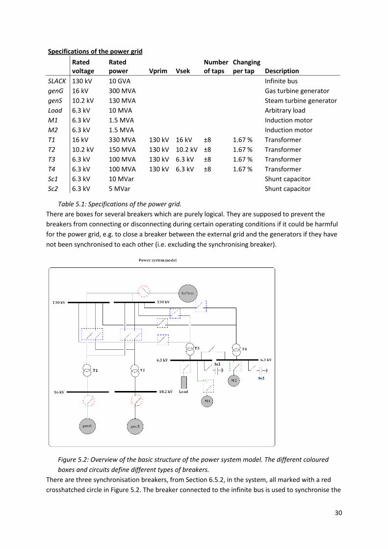
30
Specifications of the power grid
Rated
voltage
Rated
power Vprim Vsek
Number
of taps
Changing
per tap Description
SLACK 130 kV 10 GVA
Infinite bus
genG 16 kV 300 MVA
Gas turbine generator
genS 10.2 kV 130 MVA
Steam turbine generator
Load 6.3 kV 10 MVA
Arbitrary load
M1 6.3 kV 1.5 MVA
Induction motor
M2 6.3 kV 1.5 MVA
Induction motor
T1 16 kV 330 MVA 130 kV 16 kV ±8 1.67 % Transformer
T2 10.2 kV 150 MVA 130 kV 10.2 kV ±8 1.67 % Transformer
T3 6.3 kV 100 MVA 130 kV 6.3 kV ±8 1.67 % Transformer
T4 6.3 kV 100 MVA 130 kV 6.3 kV ±8 1.67 % Transformer
Sc1 6.3 kV 10 MVar
Shunt capacitor
Sc2 6.3 kV 5 MVar
Shunt capacitor
Table 5.1: Specifications of the power grid.
There are boxes for several breakers which are purely logical. They are supposed to prevent the
breakers from connecting or disconnecting during certain operating conditions if it could be harmful
for the power grid, e.g. to close a breaker between the external grid and the generators if they have
not been synchronised to each other (i.e. excluding the synchronising breaker).
Figure 5.2: Overview of the basic structure of the power system model. The different coloured
boxes and circuits define different types of breakers.
There are three synchronisation breakers, from Section 6.5.2, in the system, all marked with a red
crosshatched circle in Figure 5.2. The breaker connected to the infinite bus is used to synchronise the

31
external power grid to the power plant, while the breakers closest to the generators are used to
synchronise each generator to the internal power grid. All the other breakers in the system are
different kinds of protection breakers, explained in Section 6.5.2, except for the breaker between the
two 6.3 kV busbars, which is just a normal breaker smooth from Section 6.5.2.
In the model there are also protection equipment included, which are not visible in the overview
showed in Figure 5.2. However, the synchronisation breakers are equipped with frequency
protection, i.e. both for the single generators and for the entire power system. To the breakers
marked with a blue crosshatched box there are current protection and protection against over
magnetisation for the transformers connected. The breakers marked with a green crosshatched box
there are over and under voltage protection connected in order to protect the loads. The generator
breakers are equipped with protection against reversed power, and over and under voltage.
5.1.2 Control model
The control model basically consists of in and out ports connected to the power system model and
behind that an algorithm accountable for the performance of the power system model. Below
follows a brief description of the systems’ behaviour, which is in compliance with the considerations
made in the chapters above.
5.1.2.1 Start-up of the system
In order to start-up the system the external grid has to be connected via the synchronisation breaker.
At this moment, all the synchronisation requirements described in Section 3.2.2.1.3 do not have to
be fulfilled since the generators are off. To be able to start the generators, the motors to the pumps
and fans have first to be started in order to start the process, even though this is not a requirement
for the power system alone. When this is done the gas turbine can be started. The steam turbine
cannot be started before the gas turbine since the steam flow is produced by the exhaust gases from
the gas turbine as described in Section 1.2.
When synchronising a generator to the power grid, the control strategy for that generator has to be
voltage and frequency control, but whilst the generator is connected the control mode can transcend
to active and reactive power control. The set point for the active power can be set when the control
mode has changed. In this system the set point is applied simultaneously as the voltage regulation is
changed to reactive power control, which occurs some time after the frequency control has changed
to active power control. The time delay is due to let the system stabilise before changing the set
point. The strategy just described applies to both generators.
5.1.2.2 Normal operation
Having the gas turbine or both of the generators connected to the power system, and on the same
time having the plant connected to the external power grid implies normal operation. At this point
the tap changers on the transformers could be in automatic mode if desirable. When the steam
turbine has been connected to the power system, the turbine governor should be possessed by a
pressure controller in the steam net accounting for keeping the right pressure of the steam line. This
is going to be performed by a switch selecting the minimum value of the two controllers in the steam
net, and is beyond the limitations of this thesis. However, it has to be remembered that the steam
turbine has limited production capacity.

32
Further, when the system is in normal operation it is possible for the system operator to change
certain things in the system, like set point for the active power, control strategy for the generators
and if the tap changing of the transformers should be automatic or manual.
5.1.2.3 Island operation
If the synchronisation breaker closest to the external grid (the net breaker) disconnects, or the two
breakers below both disconnects so there is no connection between the external grid and the power
plant, the system automatically change over to island operation. In order for the system to handle
the large loss of load, going from full production about 400 MVA to support about 15 MVA internal
consumption, the valve to the gas turbine closes instantly and remain there for about 0.5 seconds
before the turbine governor controls again. However, this automatic is eligible and can therefore be
removed if not desired. To increase the control capacity of the turbine governor further, the
parameters are also changed at the same time. A new set point for the active power will be set and is
related to what the internal power consumption is at the point the system change over to island
operation. Since the gas turbine will produce a very small amount of exhaust gases the steam flow
will also be very low. Therefore, after some considerations in cooperation with the project manager,
[22], we decided to automatically turn off the steam turbine when changing over to island operation.
In order to handle this in the steam net the steam flow to the turbine is bypassed. This embedded
automation can easily be removed if desired.
During island operation the control strategy for the generator has to be voltage and frequency
control. If there are two generators trying to control the system, one or both of them have to be
equipped with some droop. In this system, where there is only one generator active during the island
operation it is eligible to have frequency or frequency/active power control. Further, the tap
changers on the transformers are changed automatically to manual operation, since they also will try
to control the voltage which is already performed by the generator. Also during island operation it is
possible for the system operator to change certain things in the system.
5.1.2.4 Resynchronisation to the external power grid
To resynchronise the power plant to the external power grid a closing signal has to be sent to the
circuit breaker closest to the external power grid. In order to fulfil the synchronisation requirements
described in Section 3.2.2.5.2, the strongest generator in the system has to be adjusted. In this case
that is the gas turbine generator, and its synchronisation system is used in the same way as when the
generator itself is synchronised to the system. The difference this time is that the voltage and
frequency values are coming from the net breaker instead of from the synchronisation breaker of the
generator. Therefore the generator also has to remain in the voltage and frequency control strategy,
which can change when the external power grid is reconnected and normal operation regained.
5.2 The complexity of the model and computing time
In order to perform the simulations in real time the fixed step iterative method Runge-Kutta of order
4, Rkfix4, will be used. For the system to be able to have simulations close to real time the step size
has to be as large as possible.
Real time simulations could be performed with the following settings:
- Method: Rkfix4
- Tolerance: 0.001

33
- Fixed integrator step: 0.01
The fixed integrator step is still a bit too large since the power system later will be integrated into the
entire simulator, which makes the system become much more complex. Therefore further
improvements can be made regarding the step size by identifying the events that requires small step
sizes, and then scale and decrease the number of events happening simultaneously.
5.3 Problems and limitations
The steam nets connected to the power system model which symbolises the turbines are only
simplifications of the real steam net system. Therefore there have been some problems with the
initiations in them, which influence the power production of the generators. There is also a
phenomenon related to this when the generators are turned off. The turbine valve is then closed, but
the valve model is equipped with a leaking property making the turbine to still produce some torque
which is sent to the generator. However, this is a very small amount and can therefore be neglected.
The leaking property is also possibly what makes the generator frequency to remain at around 49 Hz
even though the generator is turned off and supplied with a mechanical friction loss. However, the
mechanical friction is dependent on the speed of the turbine, which implies less friction during shut
down.
As will be described in Section 6.5.2 the breakers are approximated with different resistors to
symbolise open or closed position. This may contribute to a small leakage of current and voltage
through the system. However, this leakage is very small and is therefore neglected in the analysis.
This model does not have the possibility to control according to the power factor. However this could
easily be attained if desired, but have been neglected in this thesis since it is similar to the control of
the reactive power. Neither have all power plants the possibility of power factor control.
As described in Section 5.1.2 the steam turbine is shut off automatically when changing over to island
operation in order to avoid trip of the whole system. This is due to the relatively small internal power
consumption of the power plant, which is just reasonable since the main purpose of the power plant
is to produce electricity.

34
6. Models of components in the power system As mentioned in the method, models for many of the power system components have already been
developed in an earlier Master of Thesis [2] and available in the PowerSystem Library. Some of these
components will need some modification or development to be applied in this power system model.
Therefore only the modified or developed components will be described more in detail, while the
others only will be mentioned with further reference to [2].
The modelling is performed for a one phase system, due to the assumed symmetry mentioned in
Section 3.2.1.1. Further, as stated in [2], one of the fundamental conditions for computation in the
power system is to enable flow of complex voltage and current, and is provided by electrical
connectors, pins.
6.1 Generators
From the PowerSystem Library, the partial model Generator is used without any modification. This
model, which describes the complex power produced by the generator, is extended and used in the
model Slack and SynchronousGenerator.
The Slack is a model to symbolise an infinite bus modelled as an infinitely large generator and is used
as a reference for the transmission angle in the power system. As with the infinite bus the Slack
should also make it impossible to for a single generator unit connected to it to adjust the frequency.
This model is also applied without any modifications. However, for the model SynchronousGenerator
some small modifications have been performed, and due to its importance in the system it will be
further described below.
6.1.1 Synchronous generator
The model of the synchronous generator is the most complex model in the power system. The
requirements of the model include the possibility to describe the transient responses of the
generator without becoming too complex and therefore not possible to perform simulations in real
time. The model is developed with the following simplifications and assumptions according to [2]:
- The capacitance of the windings are assumed to be zero
- Every winding is represented by one concentrated winding, independent of the original
shape
- The change of the inductance in the stator windings due to the position of the rotor is
assumed to be sinusoidal and without any harmonics present
- Losses due to hysteresis and eddy currents are neglected
- The speed of the rotor is assumed to be close to the synchronous speed in the transient state
- The subtransient region is not included in the model
When a fault occurs somewhere in the system, large currents appear in the stator of the generator,
which induces currents in the rotor windings and makes the generator act as a transformer [10].
Some of these currents decay faster than others, which motivates a separation of the machine
parameters into three states: subtransient, transient, and synchronous (or steady state). The
subtransient machine parameters are associated with the rapidly decaying components, the
transient parameters with slowly decaying components, and the synchronous parameters influence
the almost constant components. The components in the synchronous generator influenced by this
separation are the effective inductances (or reactances) seen from the terminals of the generator,

35
and their corresponding time constants which describes the rate of change of the currents [7]. If the
model should represent a full scale dynamic model of a synchronous generator, all three of the states
must be included. However, by including new states the order of the model increases and hence
impairs the capacity to perform real time simulations. This is especially true for the subtransient
machine parameters, where the corresponding time constants are extremely small and therefore
requires small steps for numerical integration. Further, the model is supposed to be applied in a
simulator for operators at power plants and the subtransient time constants are too small to see in
real time operations. Thus, these can only be investigated afterwards. Their impacts have therefore
been considered to be too small for the purpose of this thesis in comparison with the increase of
model complexity, and are therefore neglected [23].
Also some transient time constants are neglected for the same reasons and also because they are not
likely to occur in this sort of model. However, the model includes dynamic for stationary states and
the transient state for no-load operation [2].
In steady state a turbo generator with non-salient pole rotor can be represented by a simple
equivalent circuit for one phase, see Figure 6.1, where is the terminal voltage, the winding
resistance (one phase), the terminal current, the field voltage which is the voltage induced in
one phase of the rotating magnetic field from the rotor, and . the synchronous
reactance (one phase) which consists of the magnetisation reactance and the leakage reactance
[7][11]. From this, the following expression for the terminal voltage can be derived:
F Equation 6.1
Figure 6.1: Equivalent electrical circuit for a synchronous generator with non-salient pole
rotor.
Another main issue when analysing power system stability is the equation of rotational inertia. The
rotational speed of the rotor has a dynamic behaviour which originates from the imbalance between
the mechanical and electromagnetic torque of the synchronous machine. The imbalance can be
described by the so called swing equation:
GH8I
H J J# Equation 6.2
where G is the combined moment of inertia of generator and turbine [kg*m2], K the mechanical
angular velocity of the rotor [rad/s], J the mechanical torque [Nm], and J# the electromagnetic

36
torque [Nm]. In order to have a combined moment of inertia for the generator and the turbine, they
have to be mounted on the same axis, which is the case for the generators and turbines concerned in
this power system [7].
In this model the normalised moment of inertia, the inertia constant L [s] defined in Equation 6.3, is
used and are usually between 2-10 s for thermal units. In the equation the combined moment of
inertia of generator and turbine, G [kg*m2], is normalised with the rated mechanical angular velocity
K [rad/s] and the base apparent power MN#. L can be seen as the time it will take the
generator to brake from synchronous speed when loaded with rated load and the power supplied is
reduced to zero [7].
L
O8PI"
QRST9U
Equation 6.3
In order to include the damping effects of damper windings, or rotor eddy currents in the turbo
generator case, in a rather simple way it is often desirable to introduce a damping factor VW into the
swing equation proportional to the speed deviation [7].
The only difference made from the original model developed by [2] is the introduction of a friction
factor representing a mechanical loss. The friction loss is an eligible percentage loss, X=>77, at full
speed and full power, stated in Equation 6.4, where J is the mechanical torque, J%& is
the torque produced by the turbine, and X* the angular speed in pu. Other losses associated with
electricity are already included in the model through the winding resistance .
J J%& X=>77 X* Equation 6.4
6.1.2 Excitation system
There exists many different types of automatic voltage regulator (AVR) models on the market, and it
is therefore better to create a general model which can easily be adjusted to the specific case [24].
From the Södra Cell Mörrum (SCM) simulator the model ExciterQcontrolDroop represents a
generator exciter equipped with an AVR. According to [2] the construction is corresponding to
common controllers in the power system, and is mainly a limited PI (Proportional-Integral) controller
with an antiwindup function for the integrating part. However, the exciter also has a PI controller for
reactive power control, which allows the exciter having two control modes: voltage regulation and
reactive power control. The voltage and reactive power are measured at the generator terminals and
used to adjust the field current supplied to the generator. The voltage regulation always contributes
to the controlling, while the reactive power control is supposed to be slower, more like “added
above”. Typical time values are some seconds for the voltage regulator and around 15-20 times
longer for the reactive power controller. During synchronisation the controller has to be in voltage
regulation mode in order to adjust the voltage magnitude to the correct value. During normal
operation the control strategy can be either of the two, but in island operation at least one of the
generators in the system has to have voltage regulation. To enable more than one generator to be
connected to the same busbar, the model has a voltage “droop” feature which is related to the
reactive power values.
In the PowerModel Library there exist two other types of excitation systems: Exciter and
ExciterQcontrol. These are plain AVRs and AVRs with added reactive power control respectively.

37
The model used in this thesis is the ExciterQcontrolDroop with some modifications. The modifications
made are some per unit scaling which has been added in order to make sure that the right reference
voltage level is used depending on the type of synchronisation performed. This is because the gas
turbine is also used to synchronise the entire power plant to the power grid after island operation.
The per unit scaling is also better from an error-analysis point of view as discussed in Section 3.5.2.
Another modification is that the voltage droop feature is removed since the two generators in the
system are placed on different busbars, but it can easily be reintroduced again.
6.1.3 Turbine governor
The turbine governor used in this model is based on the model SimpleGovernorPID from the
PowerSystem Library. This model has the basic structure showed in Figure 6.2. The main purpose of
the governor is to control the active power produced by adjusting the valve opening to the turbine,
hence control the frequency in the system. As Figure 6.2 shows the model represents a PID
(Proportional-integral-derivative) controller, which is also equipped with an antiwindup function for
the integrating part. The index 0 on the frequency and the active power symbolise reference values
which are adjustable during operation, while N# represents the rated active power of the
generator. is the static droop, which enables feedback of the active power. The statics is inversely
proportional to the power frequency characteristic, i.e. when the statics is zero the power frequency
characteristic is infinite. However, the statics is necessary when there is more than one generator in
the system.
Figure 6.2: Basic structure of a turbine governor with feedback of active power.
Figure 6.2 also shows one of many ways to construct a PID-controller, where this way has been
common due to the simpler construction. Instead of having the PID-parts in parallel it is also common
to have the P-part before and then the I- and D-part in parallel which theoretically is simpler. Either
way can be used, and the only difference from a modelling point of view is to remember that the
parameter values are different.
In some power plants the parameters of the controller automatically change during island operation
in order to have a stronger and faster control of the frequency. This is also applied in the model
developed in this thesis, since it provides a better change over to island operation. However, the
parameters are set by the user and the effect is therefore eligible.

38
6.1.4 Synchronisation controller
The synchronisation system connected to the synchronisation breaker in the generator is a PID
controller used to control the reference frequency at the turbine governor, provided from the
PowerSystem Library. The controller used in the steam turbine is used without any modification,
while the gas turbine has a slightly adjusted version. The controller is turned on when the generator
is in the synchronisation phase with the angular difference between the generator and the grid used
as reference signal.
The modifications made in the gas turbine controller are due to the usage of this controller when
resynchronising the external power grid to the power plant. The modifications made are change of
angular difference reference signal during this synchronisation to be the difference between the
external power grid and the power plant, and simultaneously change of parameters in the controller.
6.2 Transformers
The transformers used in this thesis are a simplified version of a single-phase two winding
transformer, provided from the PowerSystem Library, which is developed according to the theory
mentioned in Section 3.2.2.2 [2]. By simplified version means that the parameters included are only
the short circuit resistance and the short circuit reactance, Y and Y, hence knowledge about both
short circuit and open circuit tests are not needed. Further, the no-load current is approximated to
zero, hence the iron and magnetising losses are neglected (' and from Figure 3.6). The values
should be given in per unit.
There are two versions of the simplified two winding transformer: one has the possibility to control
the turning ratio with a tap changer and one has fixed turning ratio. The transformer used in this
power system model is the one with control possibility. Both transformer models have different
connection setups: Y-Δ, Δ-Y, Δ-Δ and Y-Y.
The transformer model does not include any transient behaviour since it, as mentioned earlier in
Section 3.2.2.3, seldom influence the electromagnetically phenomenon significantly [6].
6.2.1 Tap changer
From the PowerSystem Library a model representing a discrete tap changer, Stepwise TCUL (Tap
Changing Under Load) Regulator, were obtained and used without any modifications together with a
model over a simple controller transformer, described above. The controller symbolise a controller
with discrete behaviour even though the underlying functions are continuous. A potential sensor is
used to compare apparent voltage with rated value. If the voltage deviation is larger than given dead
zone, a signal is sent to the transformer depending on time delay characteristic. The out signal have
pulsed increases or decreases as an approximation of a discrete signal [2].
The tap changing can be automatic during normal operation, but when the power plant is in island
operation it should be manually controlled by the operator. The tap changer will otherwise try to
control the voltage level of the generator, which is not possible during island operation since the
voltage level in the system is then decided by the generator.
6.3 Loads
From [2] and the PowerSystem Library a model representing a constant impedance load was already
developed. This model has a power consumption proportional to the voltage squared, and can be an
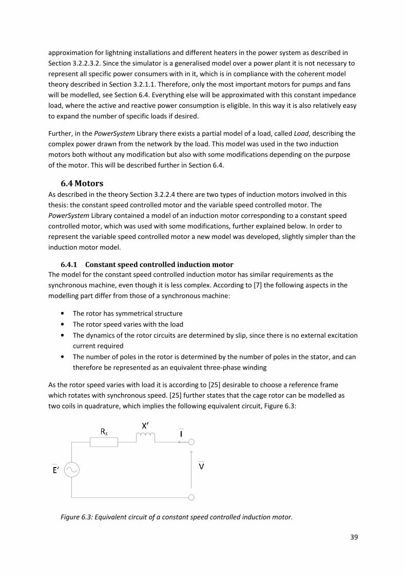
39
approximation for lightning installations and different heaters in the power system as described in
Section 3.2.2.3.2. Since the simulator is a generalised model over a power plant it is not necessary to
represent all specific power consumers with in it, which is in compliance with the coherent model
theory described in Section 3.2.1.1. Therefore, only the most important motors for pumps and fans
will be modelled, see Section 6.4. Everything else will be approximated with this constant impedance
load, where the active and reactive power consumption is eligible. In this way it is also relatively easy
to expand the number of specific loads if desired.
Further, in the PowerSystem Library there exists a partial model of a load, called Load, describing the
complex power drawn from the network by the load. This model was used in the two induction
motors both without any modification but also with some modifications depending on the purpose
of the motor. This will be described further in Section 6.4.
6.4 Motors
As described in the theory Section 3.2.2.4 there are two types of induction motors involved in this
thesis: the constant speed controlled motor and the variable speed controlled motor. The
PowerSystem Library contained a model of an induction motor corresponding to a constant speed
controlled motor, which was used with some modifications, further explained below. In order to
represent the variable speed controlled motor a new model was developed, slightly simpler than the
induction motor model.
6.4.1 Constant speed controlled induction motor
The model for the constant speed controlled induction motor has similar requirements as the
synchronous machine, even though it is less complex. According to [7] the following aspects in the
modelling part differ from those of a synchronous machine:
• The rotor has symmetrical structure
• The rotor speed varies with the load
• The dynamics of the rotor circuits are determined by slip, since there is no external excitation
current required
• The number of poles in the rotor is determined by the number of poles in the stator, and can
therefore be represented as an equivalent three-phase winding
As the rotor speed varies with load it is according to [25] desirable to choose a reference frame
which rotates with synchronous speed. [25] further states that the cage rotor can be modelled as
two coils in quadrature, which implies the following equivalent circuit, Figure 6.3:
Figure 6.3: Equivalent circuit of a constant speed controlled induction motor.

40
where 2Z is a transient emf (vector), Z a transient impedance and the stator resistance. The
induction motor from the PowerSystem Library is constructed according to this equivalent circuit.
This model was used with some smaller modifications, like adding a mechanical friction factor in the
same way as with the synchronous generator. Another modification made was to move the load
torque characteristics outside the motor model in order to connect it to the correct pump or fan
model in the steam net later on. Now the load torque characteristics are given by the following
approximation:
J[
QR\# ,M
8"
89" . ]
8
89. ^0
Equation 6.5
where 0 is active power drawn by the motor, M]@7 the rated apparent power, K the angular
frequency, and K the rated angular frequency (synchronous speed). A, B and C are all parameters
determining the characteristics. For example, centrifugal pumps are normally characterised by a
squared relationship (A), machine tools by a proportional relationship (B), and overhead cranes
normally have constant torque dependence.
As maybe noticed, the number of poles in the motor is not included in the model. However, since this
is mainly a scale factor and not important for the performance of the model, it has been neglected
but can easily be included if desired.
The model is, as recalled from the synchronous generator model above, constructed with a partial
model, Load, determining the power drawn from the power grid as mentioned in Section 6.3.
However, as seen in Equation 6.5 the reactive power drawn is not explicit calculated, but is
instead determined by the motor operating point.
6.4.2 Variable speed controlled induction motor
The variable speed controlled induction motor is a slightly simplified version compared to the
constant speed controlled motor above. The model uses Load, described in Section 6.3, as partial
model and connected to it are a simple induction motor model together with a frequency converter
with torque limiter. As with the induction motor described above, this model also has the pump
characteristic as an external model.
The working principle of the motor is as follows. The controller in the steam net model, which is
supposed to control the steam pressure after the pump, sends a signal to the motor of a desired
rotational speed (i.e. the pump). Corresponding mechanical rotational speed is sent to the pump
model which responds with a mechanical torque depending on its characteristics. The corresponding
electrical torque is then used to calculate the amount of electrical power drawn from the power grid.
However, in order to prevent the pump for drawing too much power, i.e. more than the motor can
supply, there is a torque limiter embedded in the frequency converter. It is supposed to decrease or
increase the mechanical rotational speed if the electrical torque becomes too large or too small.
This is something that should work, at least in theory. However, it has not been possible to make the
model to work properly in Dymola, probably due to the way Modelica performs the calculations.
Another solution which can be used instead is to have a continuous gear between the pump and
pump controller and the constant speed controlled motor model.

41
6.5 Transmission net, breakers and shunt capacitors
6.5.1 Transmission line
As mentioned in Section 3.2.2.5.1 the transmission lined concerned in this thesis is the long overhead
power line, which can be represented by the equivalent π-circuit, seen in Figure 3.9. The model
available in the PowerSystem Library was created from existing components of impedance and
admittance. The only modification made in this component is a clarifying of the parameter values,
where the user can chose between giving values in Ohm and Siemens, or in per unit.
6.5.2 Breakers
From the PowerSystem Library several models of different breakers were obtained, all originated
from the same basic model. According to [2] it is difficult to represent a breaker due to the way
Modelica perform the calculations, and the solution is to have a resistor in series with the ports
varying between a very small and a very large value depending on if the breaker is closed or open.
The very large value is an approximation of the infinite resistance that occurs when a line is opened.
In order to decide open or closed position one or several boolean ports are connected to the
breaker.
The following are some of the breakers existing in the PowerSystem Library, along with the
description of the breakers developed during this thesis:
BreakerSmooth
A breaker with smooth transition between open and closed, connected to the same boolean port, i.e.
the breaker can be 50% open and 50% closed since the resistor is a function of the transition. This
breaker is the base for the rest of the breakers.
ProtectionBreaker
Have the same basic features as the BreakerSmooth. Here several boolean ports are connected to
the Open and Close commands, which can be controlled manually or by protection devices. Several
types were created where only the number of ports differs, which depends on where in the power
system they are applied.
SynchroBreaker
This is a generator breaker and a part of the synchronisation system consisting of a main breaker and
an earth breaker (BreakerSmooth) connected to ground in order to simplify voltage reduction during
open position. This breaker does not close immediately when a closing signal is sent, instead a set of
conditions have to be fulfilled first: voltage difference, angle difference, and derivative of angle
difference must be within certain limits.
In order to simplify transition between island operation and normal operation of the power plant, a
synchronising breaker was developed as a net breaker also. The difference between this and the
original is mainly an additional boolean port for the net breaker deciding if the breaker can be closed
without fulfilling the conditions stated above, which is the case when the power plant is to be started
up.

42
6.5.3 Shunt capacitance
The ShuntCapacitance in the PowerSystem Library is made of admittance in series with ground,
where the conductance G set to zero, which leaves the susceptance B to be purely capacitive. The
power produced by the shunt capacitor will only be reactive and varies with voltage level. No
modification was made to the component used in this thesis.
6.6 Protection systems
The protection system used here are simple logical components which are connected to the
protection breaker explained in Section 6.5.2.
6.6.1 Current protection
The current protection used in this thesis is an upgraded version of the current protection device
from the PowerSystem Library. It is a simple logical component protecting the system against over
current if activated. The component gets a signal input from a current sensor, which is compared
with a maximum value. If the maximum value is exceeded by the measured value and the component
is activated (by a boolean signal), a signal is sent to a breaker to open after some time delay. This
version also indicates at a value lower than the maximum value in order to alert the operators. All
current threshold values and the time delay are set by the user.
6.6.2 Voltage protection
Two versions of the voltage protection device were developed in this thesis, one placed to protect
the generators and one for the motors. They have the same properties as the current protection
device explained above, but protection against both over and under voltage. The only thing that
differs between the two versions is an extra input signal for activation of the component placed to
protect the generator.
6.6.3 Frequency protection
As mentioned in Section 3.2.2.6.3, to provide frequency protection for the system as a separate
component is not necessary since the frequency of the system is decided by the external power grid
or, during island operation, by the strongest generator, and the protection can therefore be
connected to the generator breakers or the net breaker. For the generators the frequency protection
is most important during island operation, since during normal operating conditions the external
power grid is too strong for single generators to disturb.
Two different frequency protection systems is therefore setup, one for the single generators and one
for the entire power system. The protection for single generators has two limits for over-frequency
protection and one limit for under-frequency protection. The limits and the associated time limits are
decided by the user. The protection for the power system has only one limit for over-frequency and
one for under-frequency since these also are much more unlikely to occur.
6.6.4 Magnetisation protection
The magnetisation protection was developed in order to protect especially transformers from being
over magnetised, as described in Section 3.2.2.6.4. As for the current protection above, the
magnetisation protection device also has one indicating value and maximum breaking value. Here
two signals are coming in: voltage magnitude from a voltage sensor and frequency value from the
closest generator. These values are normalised and compared with values set by the user.

43
6.6.5 Reversed power protection
The reversed power protection protects the generator from power flowing in the wrong direction as
described in Section 3.2.2.6.5. It gets signal input from a power sensor which is compared with an
indicating and a maximum value, as for the other protection devices. This protection is mainly
supposed to be used for the generator, which requires two activate signals as for the voltage
protection.

44
7. Results of simulations All graphs presented in the results below have time in seconds represented along the x-axis. The
parameters of the components have been chosen to present arbitrary standard components and a
realistic behaviour of the model or models. The most important parameters will be presented in each
section.
7.1 Validation of components
7.1.1 Start-up of a constant speed controlled induction motor
In this section results from start-up dynamics of a constant speed controlled induction motor are
showed. The induction motor has the following parameter values:
Parameter Value Description
P [W] 9,00E+05 Rated load active power
Q [VAr] 8,00E+05 Rated load reactive power
VnBase [V] 6300 Rated voltage
VABase [VA] 1,50E+06 Rated apparent power
wloss [1] 0,02 Friction loss, percentage at full power and speed
rs [pu] 0,01 Stator resistance
xs [pu] 0,11 Stator reactance
rr [pu] 0,04 Rotor resistance
xr [pu] 0,12 Rotor reactance
xm [pu] 4 Magnetising reactance
H [s] 1 Inertia constant
Table 7.1: Parameter values of the induction motor.
The load characteristics for this case are a simple pump representation, i.e. M 1 in: J[
QR\#
,M 8"
89" . ]
8
89. ^0, Equation 6.5.
The motor is started by closing the breaker at time 10. Figure 7.1 shows the characteristic start-up
dynamics of an induction motor where the reactive power drawn by the motor is much larger than
the active power at first. The reason to this phenomenon during the start-up is due to the
magnetisation of the rotor, explained in Section 3.2.2.4. The starting sequence is over once the rotor
has reached its rated rotational speed.
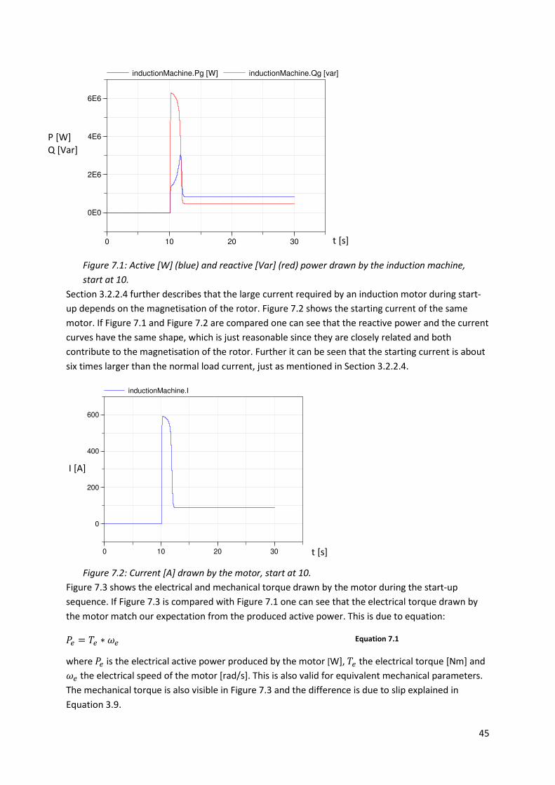
45
dsC
Figure 7.1: Active [W] (blue) and reactive [Var] (red) power drawn by the induction machine,
start at 10.
Section 3.2.2.4 further describes that the large current required by an induction motor during start-
up depends on the magnetisation of the rotor. Figure 7.2 shows the starting current of the same
motor. If Figure 7.1 and Figure 7.2 are compared one can see that the reactive power and the current
curves have the same shape, which is just reasonable since they are closely related and both
contribute to the magnetisation of the rotor. Further it can be seen that the starting current is about
six times larger than the normal load current, just as mentioned in Section 3.2.2.4.
Figure 7.2: Current [A] drawn by the motor, start at 10.
Figure 7.3 shows the electrical and mechanical torque drawn by the motor during the start-up
sequence. If Figure 7.3 is compared with Figure 7.1 one can see that the electrical torque drawn by
the motor match our expectation from the produced active power. This is due to equation:
# J# K# Equation 7.1
where # is the electrical active power produced by the motor [W], J# the electrical torque [Nm] and
K# the electrical speed of the motor [rad/s]. This is also valid for equivalent mechanical parameters.
The mechanical torque is also visible in Figure 7.3 and the difference is due to slip explained in
Equation 3.9.
0 10 20 30
0E0
2E6
4E6
6E6
inductionMachine.Pg [W] inductionMachine.Qg [var]
0 10 20 30
0
200
400
600
[A]
inductionMachine.I
t [s]
t [s]
P [W] Q [Var]
I [A]

46
Figure 7.3: Electrical torque (Te, blue) and mechanical torque (Tm, red) [pu], start at 10.
The slip s is also observable is Figure 7.4 which shows the mechanical rotor speed (w) and the
synchronous rotor speed (wsync).
Figure 7.4: Rotor angular speed (w, blue) of the motor together with the synchronous angular
speed (wsync, red) [rad/s], start at 10.
7.1.2 Start-up of a generator
The generator (represented by the gas turbine in this case) has the following parameter values:
Parameter Value Description
P [W] 3E+8*0,9 Rated active power generation
VAbase [VA] 3,00E+08 Rated apparent power
VnBase [V] 1,60E+04 Rated voltage
wloss [1] 0,01 Friction loss, percentage at full power and speed
wstart [rad/s] 2*pi*45 Start value of angular speed
ra [pu] 0,0035 Armature resistance
xd [pu] 1,65 Direct axis synchronous reactance
0 10 20 30
-0.5
0.0
0.5
1.0
1.5
2.0[p
u]
inductionMachine.Te inductionMachine.Tm
0 10 20 30
0
100
200
300
[rad
/s]
inductionMachine.w inductionMachine.wsync
t [s]
t [s]
w [rad/s]
T [pu]

47
xq [pu] 1,65 Quadrature axis synchronous reactance
xdp [pu] 0,25 Direct axis transient reactance
Td0prim [s] 8,5 Open-circuit direct axis transient time constant
H [s] 8,28 Inertia constant
Kd [1] 3 Damping coefficient
Table 7.2: Parameter values of the gas turbine generator.
Before started, at time 50, the generator has a rotational speed (frequency) of 45 Hz. This is due to
problems with the calculations in the program and initiations. The starting sequence begins with an
increase of the frequency to about 50 Hz, see Figure 7.5, by increasing the torque from the turbine.
Whilst the generator is close to nominal speed the voltage magnitude is increased by magnetisation
of the rotor, visible in Figure 7.6. When both the frequency and the voltage are close to their nominal
values the synchronisation with the external power grid may start, and the values are slightly
adjusted in order to fulfil the synchronisation requirements described in Section 3.2.2.1.3.
At time 142 the generator has been synchronised to the grid and the breaker is closed. At this point,
i.e. when the breaker closes, a small oscillation is noticeable on the curve in Figure 7.5. Recalling
Section 3.2.1.2 this is an example of when the generator is displaced from its equilibrium point and
the rotor angle starts to oscillate around it. Since the oscillation declines the system can be seen as
stable.
Figure 7.5: Electrical frequency [Hz] of the generator, start at 50, synchronised to the power
grid at time 142.
10 seconds after being synchronised the control strategy of the generator is changed from frequency
control to active power control, and 30 seconds after that the voltage regulation is changed to
reactive power control. The reason for the time delay between the two events is to let the system
stabilise. The change from voltage regulation to reactive power control is observable in Figure 7.6
around time 200 when the voltage level starts to differ from the reference voltage level.
0 40 80 120 160 200 240 280
45
46
47
48
49
50
51
[Hz]
PowerNet.genG.f
t [s]
f [Hz]

48
Figure 7.6: Voltage magnitude of the generator clips (V) together with the voltage reference
value (Vref), both in [V]. Generator started at 50, changed over to reactive power control
around time 180.
Simultaneously as the reactive power control is activated the reference value for the active power
production is changed, visible in Figure 7.7. The oscillation from Figure 7.5 is closely related to the
oscillation appearing in Figure 7.7, since the frequency and the active power of the generator are
closely related.
Figure 7.7: Active power (P_out, blue) and reactive power (Q_out, green) produced by the
generator in [W] and [VAr] respectively, together with the active power reference value
(P_ref, red) in [W]. Generator synchronised to the power grid at time 142, changed over to
reactive power control around time 180 simultaneously as the active power reference value is
changed.
Before the activation of the reactive power control the generator consumed reactive power, seen in
Figure 7.7, i.e. the generator was under magnetised. This explains why the voltage in Figure 7.6
increases when the reactive power control is activated, i.e. the generator requires reactive power to
fully magnetise the rotor since the rated voltage probably is slightly too low.
0 40 80 120 160 200 240 280
0.0E0
2.0E3
4.0E3
6.0E3
8.0E3
1.0E4
1.2E4
1.4E4
1.6E4
PowerNet.genG.G.V [V] PowerNet.genG.Exc.Vref
0 40 80 120 160 200 240 280-5.0E7
0.0E0
5.0E7
1.0E8
1.5E8
2.0E8
2.5E8
3.0E8
3.5E8PowerNet.genG.G.P_out PowerNet.genG.Gov.P_ref PowerNet.genG.G.Q_out
t [s]
t [s]
P [W] Q [Var]
U [V]
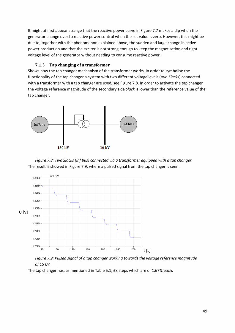
49
It might at first appear strange that the reactive power curve in Figure 7.7 makes a dip when the
generator change over to reactive power control when the set value is zero. However, this might be
due to, together with the phenomenon explained above, the sudden and large change in active
power production and that the exciter is not strong enough to keep the magnetisation and right
voltage level of the generator without needing to consume reactive power.
7.1.3 Tap changing of a transformer
Shows how the tap changer mechanism of the transformer works. In order to symbolise the
functionality of the tap changer a system with two different voltage levels (two Slacks) connected
with a transformer with a tap changer are used, see Figure 7.8. In order to activate the tap changer
the voltage reference magnitude of the secondary side Slack is lower than the reference value of the
tap changer.
Figure 7.8: Two Slacks (Inf bus) connected via a transformer equipped with a tap changer.
The result is showed in Figure 7.9, where a pulsed signal from the tap changer is seen.
Figure 7.9: Pulsed signal of a tap changer working towards the voltage reference magnitude
of 15 kV.
The tap changer has, as mentioned in Table 5.1, ±8 steps which are of 1.67% each.
40 80 120 160 200 240 280
1.70E4
1.72E4
1.74E4
1.76E4
1.78E4
1.80E4
1.82E4
1.84E4
1.86E4
1.88E4
[V]
inf1.G.V
t [s]
U [V]

50
7.2 Validation of power system model
7.2.1 Cold start of the system
The external power grid is connected to the power plant by closing the net breaker, and the motors
are started by closing the breakers. The induction motors shows the same behaviour as the start-up
dynamics explained in Section 7.1.1, and are therefore not necessary to show again. The
transformers supplying the motors change to automatic tap changing when the motors are
connected. All the breakers between the net breaker and the gas turbine generator are closed before
the synchronisation of the generator start ups, and the same start-up dynamics as explained in
Section 7.1.2 are attained. The gas turbine generator has the following parameter values:
Gas turbine generator
Parameter Value Description
P [W] 3E+8*0,9 Rated active power generation
VAbase [VA] 3,00E+08 Rated apparent power
VnBase [V] 1,60E+04 Rated voltage
wloss [1] 0,01 Friction loss, percentage at full power and speed
wstart [rad/s] 2*pi*45 Start value of angular speed
ra [pu] 0,0035 Armature resistance
xd [pu] 1,65 Direct axis synchronous reactance
xq [pu] 1,65 Quadrature axis synchronous reactance
xdp [pu] 0,25 Direct axis transient reactance
Td0prim [s] 8,5 Open-circuit direct axis transient time constant
H [s] 8,28 Inertia constant
Kd [1] 3 Damping coefficient
Table 7.3: Parameter values of the gas turbine generator.
As explained in Section 7.1.2, when the gas turbine has been synchronised to the grid the control
strategy changes from frequency and voltage regulation to active and reactive power control.
Simultaneously the active power production reference value is changed to rated power, 300 MW,
see Figure 7.10. The transformer connected to the gas turbine changes to automatic tap changing.
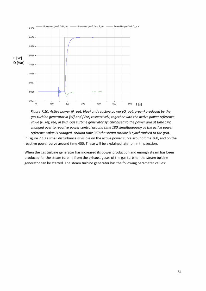
51
Figure 7.10: Active power (P_out, blue) and reactive power (Q_out, green) produced by the
gas turbine generator in [W] and [VAr] respectively, together with the active power reference
value (P_ref, red) in [W]. Gas turbine generator synchronised to the power grid at time 142,
changed over to reactive power control around time 180 simultaneously as the active power
reference value is changed. Around time 360 the steam turbine is synchronised to the grid.
In Figure 7.10 a small disturbance is visible on the active power curve around time 360, and on the
reactive power curve around time 400. These will be explained later on in this section.
When the gas turbine generator has increased its power production and enough steam has been
produced for the steam turbine from the exhaust gases of the gas turbine, the steam turbine
generator can be started. The steam turbine generator has the following parameter values:
0 100 200 300 400 500 600
-5.0E7
0.0E0
5.0E7
1.0E8
1.5E8
2.0E8
2.5E8
3.0E8
3.5E8PowerNet.genG.G.P_out PowerNet.genG.Gov.P_ref PowerNet.genG.G.Q_out
t [s]
P [W] Q [Var]

52
Steam turbine generator
Parameter Value Description
P [W] 1,3E+8*0,9 Rated active power generation
VAbase [VA] 1,30E+08 Rated apparent power
VnBase [V] 1,02E+04 Rated voltage
VABase [VA] 1,30E+06 Rated power
wloss [1] 0,01 Friction loss, percentage at full power and speed
wstart [rad/s] 2*pi*45 Start value of angular speed
ra [pu] 0,004 Armature resistance
xd [pu] 1,6 Direct axis synchronous reactance
xq [pu] 1,6 Quadrature axis synchronous reactance
xdp [pu] 0,31 Direct axis transient reactance
Td0prim [s] 6,5 Open-circuit direct axis transient time constant
H [s] 6,09 Inertia constant
Kd [1] 5 Damping coefficient
Table 7.4: Parameter values of the steam turbine generator.
The steam turbine generator has the same start-up dynamics as explained for the gas turbine
generator, with the only difference of having slightly different values. The steam turbine generator is
synchronised to the grid at time 358. The active power production reference value is changed to
rated power, 130 MW, see Figure 7.13. The transformer connected to the steam turbine changes to
automatic tap changing.
Figure 7.11: Electrical frequency [Hz] of the gas turbine generator when the steam turbine
generator is connected to the power plant.
350 360 370 380
49.98
+0.005
+0.010
+0.015
+0.020
+0.025
+0.030
+0.035
[Hz]
PowerNet.genG.f
t [s]
f [Hz]

53
Figure 7.12: Electrical frequency [Hz] of the steam turbine generator, start at 250,
synchronised to the power grid at time 358.
As for the gas turbine generator a small oscillation occurs when the breaker of the steam turbine
generator is closed, see Figure 7.12 around time 360. This oscillation is also visible in the frequency of
the gas turbine generator, as can be seen in Figure 7.11, which is a representation for the rotor angle
displacement that occurs. The same phenomenon is the explanation for the disturbance on the
active power curve of the gas turbine seen in Figure 7.10, since a similar oscillation occurs on the
steam turbine curve, visible in Figure 7.13.
Figure 7.13: Active power (P_out, blue) and reactive power (Q_out, green) produced by the
steam turbine generator in [W] and [VAr] respectively, together with the active power
reference value (P_ref, red) in [W]. Steam turbine generator synchronised to the power grid
at time 360, changed over to reactive power control around time 400 simultaneously as the
active power reference value is changed.
Figure 7.13 further shows that the steam turbine generator starts to consume reactive power when
the active power reference value is changed and the generator starts to produce active power. The
explanation for this is the same as mentioned in Section 7.1.2, i.e. that the excitation system is not
0 250 500
44
45
46
47
48
49
50
51[H
z]
PowerNet.genS.f
0 100 200 300 400 500 600
-2.0E7
0.0E0
2.0E7
4.0E7
6.0E7
8.0E7
1.0E8
1.2E8
1.4E8PowerNet.genS.G.P_out PowerNet.genS.Gov.P_ref PowerNet.genS.G.Q_out
t [s]
t [s]
P [W] Q [Var]
f [Hz]

54
strong enough and the generator has to consume reactive power in order to maintain the
magnetisation. This consumption of reactive power is the reason for the disturbance on the reactive
power curve of the gas turbine generator in Figure 7.10, i.e. the reactive power drawn by the steam
turbine generator affects the reactive power level in the entire system.
The diagrams for the voltage magnitude for the two generators are very close to the diagram showed
in Figure 7.6.
7.2.2 Load change during normal operation
In order to demonstrate a load change during normal operation an 11.6 MW (11.65 MVA) load is
disconnected from the system by using a breaker. The same parameter settings as in Section 7.2.1
are used.
At time 500 a breaker is opened and the load is disconnected from the system. The affect on the gas
turbine generator can be seen in Figure 7.14 and Figure 7.15, which are the frequency and the active
power production of the gas turbine generator respectively. Figure 7.14 shows that the reference
level of the frequency is slightly displaced from 50 Hz, which is probably a numerical error. The affect
on the steam turbine generator is similar since they are connected, hence the gas turbine generator
can be a representation of how the entire system in the power plant react to the load loss.
Figure 7.14: Electrical frequency [Hz] of the gas turbine generator during loss of 11.6 MW
(11.65 MVA) load at time 500.
498 500 502 504 506 508
49.997
+0.001
+0.002
+0.003
+0.004
+0.005
+0.006
+0.007
+0.008
[Hz]
PowerNet.genG.f
t [s]
f [Hz]

55
Figure 7.15: Active power (P_out, blue) produced by the gas turbine generator in [W]
together with the reference value (P_ref, red) in [W] during loss of 11.6 MW (11.65 MVA)
load at time 500.
By carefully studying the scales of the diagrams, it can be seen that the occurring disturbance is
relatively small. This disturbance is a typically small signal disturbance, and as discussed in Section
7.1.2, the system can be seen as small-signal stable. The reason to why the disturbance is so small is
due to the large size of the power system, since the system in this case is the power plant and the
external power grid.
Since the disturbance is small it will not activate any of the protection systems present.
Figure 7.16: Voltage magnitude [V] of the gas turbine generator clips (V) during loss of 11.6
MW (11.65 MVA) load at time 500.
Figure 7.16 shows the voltage magnitude of the gas turbine generator during the loss of load. The
appearance is the same regardless of whether the control strategy of the generator is voltage
regulation or reactive power control. Since the load consumes some reactive power it will be a small
overbalance of reactive power in the system just after the loss, which results in a small increase in
voltage. However, it can be seen that the disturbance also here is small in comparison as explained
before.
500 510
2.95E8
2.96E8
2.97E8
2.98E8
2.99E8
3.00E8
3.01E8
3.02E8
3.03E8
3.04E8PowerNet.genG.G.P_out PowerNet.genG.Gov.P_ref
500 502 504 506
1.624E4
+2
+4
+6
+8
+10
[V]
PowerNet.genG.G.V
t [s]
t [s]
P [W]
U [V]

56
7.2.3 Trip of generator during normal operation
In this Section results from tripping the steam turbine generator during normal operation is showed.
The trip is performed by disconnecting the steam turbine generator from the power plant by opening
some breakers. The same parameter values as in Section 7.2.1 are used.
The steam turbine generator is disconnected from the power plant at time 550, which means that
the generator loses its entire load. When the load is lost for the turbine, the rotor will start to over
speed since there is nothing holding back the incoming torque from the turbine, even though the
active power reference value is changed instantly due to detection of idle operation.
Figure 7.17: Electrical frequency [Hz] of the steam turbine generator when disconnected from
the power plant at time 550.
However, Figure 7.17 shows what happens with the frequency of the steam turbine generator during
the load loss. As explained in Section 5.1.1 there is a frequency protection system connected to the
generator, which in this case have the following parameter values:
Steam turbine generator
Parameter Value Description
fmin [Hz] 47 Minimum frequency
tmin [s] 20 Maximum time for falling below fmin
fmax1 [Hz] 52,5 Maximum frequency 1
tmax1 [s] 5 Maximum time for exceeding fmax1
fmax2 [Hz] 54 Maximum frequency 2
tmax2 [s] 1 Maximum time for exceeding fmax2
Table 7.5: Parameter values of the frequency protection system of the steam turbine
generator.
Table 7.5: Parameter values of the frequency protection system of the steam turbine generator
together with Figure 7.17 shows that the frequency protection system will disconnect the
synchronisation breaker of the generator, hence trip the generator. In addition it shows that the
frequency slows down to a value slightly below 50 Hz even though it is turned off and should go
500 600 700
48
50
52
54
56
58
[Hz]
PowerNet.genS.f
t [s]
f [Hz]

57
down to 45 Hz. This is probably caused by a too small mechanical friction, wloss in Table 7.4, in the
model in combination with leakage of steam to the turbine, hence incoming torque to the generator.
Figure 7.18: Power [W] production loss of the power plant when disconnecting the steam
turbine at time 550.
At first when the steam turbine generator is disconnected from the power plant, the rest of the
power system also see this as a loss of load, see Figure 7.18. Again the characteristic oscillation
starts.
As for the case in Section 7.2.2 the gas turbine generator will be affected, and this is showed in Figure
7.19. The oscillation that occurs is this time larger than in Figure 7.14 and Figure 7.15 since the
disturbance is much larger, but otherwise it is the same phenomenon. However, also here the
generator appears to remain stable without losing its synchronism to the power grid. One should
remember that the system losing the load in this case is the power plant together with the external
power grid.
500 520 540 560 580 600 620
2.4E8
2.6E8
2.8E8
3.0E8
3.2E8
3.4E8
3.6E8
3.8E8
4.0E8
4.2E8
4.4E8
[W]
PowerNet.P_H.P
520 540 560 580 600
49.94
49.96
49.98
50.00
50.02
50.04
50.06
[Hz]
PowerNet.genG.f
t [s]
t [s]
P [W]
f [Hz]

58
Figure 7.19: Electrical frequency [Hz] of the gas turbine generator when the steam turbine
generator is disconnected from the power plant at time 550.
The active power production of the gas turbine generator is affected in a similar way as in Figure 7.15
since the reference value is not affected due to no disconnection from the external power grid.
7.2.4 Island operation
In order to make the system change over to island operation the net breaker is opened. The same
parameter values as in Section 7.2.1 are used.
The net breaker is opened at time 550 when the system is in normal operation. When the
disconnection appears the steam turbine is automatically turned off and the valve to the gas turbine
is completely closed for 0.5 seconds before the governor continues to control. All transformers
automatically change their tap changers to manual operation, and the control strategy for the gas
turbine generator changes to frequency and voltage regulation.
Figure 7.20: Electrical frequency [Hz] of the gas turbine generator when changing over to
island operation at time 550.
Disconnecting the power plant from the external power grid can be seen as removing a large load. As
a consequence the gas turbine generator will start to over speed, which can be seen in Figure 7.20.
However, in order to avoid a trip of the entire power plant the production has to be decreased
instantly, why the steam turbine generator is turned off and the valve to the gas turbine is closed
completely for 0.5 seconds. The gas turbine generator has the same parameter values as the steam
turbine frequency protection system in Table 7.5: Parameter values of the frequency protection
system of the steam turbine generator, and since the frequency in Figure 7.20 stays below those
values the generator avoids a disconnection, i.e. a trip.
The active power production reference value, when changing over to island operation, is decided by
the internal power consumption, which is detected at the point when the power plant disconnects
from the external power grid. This can be seen clearly in Figure 7.21. However, this does not further
affect the generator since it has changed over to frequency control, and there is no droop available in
this case.
520 560 600 640 680 720
49.5
50.0
50.5
51.0
51.5
52.0
52.5
53.0
[Hz]
PowerNet.genG.f
t [s]
f [Hz]

59
Figure 7.21: Active power (P_out, blue) and reactive power (Q_out, green) produced by the
gas turbine generator in [W] and [VAr] respectively, together with the active power reference
value (P_ref, red) when changing over to island operation at time 550.
To disconnect the external power grid from the power plant may also appear as the same thing as to
have a short circuit somewhere along the power net and protection equipment disconnects the
power plant. This is certainly a transient stability problem although, as Figure 7.21 shows, the active
and reactive power is not particularly affected regarding oscillation issues. However, this is probably
due to a combination of turning off the steam turbine simultaneously as the valve to the gas turbine
is completely closed for a short time.
Figure 7.22: Voltage magnitude of the gas turbine generator clips with different parameter
setting (V1, red and V2, green) together with the voltage reference value (Vref, blue), both in
[V], when changing over to island operation at time 550.
Figure 7.22 shows a severe disturbance in the voltage magnitude for the gas turbine generator when
changing over to island operation. The reason for this large dip is due to the large load loss in
combination with that the system is more resistive than reactive. The red curve,
550 555 560
-5.0E7
0.0E0
5.0E7
1.0E8
1.5E8
2.0E8
2.5E8
3.0E8
3.5E8PowerNet.genG.G.P_out PowerNet.genG.Gov.P_ref PowerNet.genG.G.Q_out
550 551 552 553 554
1.20E4
1.25E4
1.30E4
1.35E4
1.40E4
1.45E4
1.50E4
1.55E4
1.60E4
1.65E4
1.70E4PowerNet.genG.Exc.Vref PowerNet.genG.G.V1 [V] PowerNet.genG.G.V2 [V]
t [s]
t [s]
P [W] Q [Var]
U [V]

60
PowerNet.genG.G.V1, is when the system has the same parameter values as in Section 7.2.1. The
green curve, PowerNet.genG.G.V2, is when the follow parameter values have been changed:
Gas turbine generator
Parameter Value Description
xd [pu] 1,85 Direct axis synchronous reactance
xq [pu] 1,85 Quadrature axis synchronous reactance
xdp [pu] 0,32 Direct axis transient reactance
Steam turbine generator
Parameter Value Description
xd [pu] 1,8 Direct axis synchronous reactance
xq [pu] 1,8 Quadrature axis synchronous reactance
Table 7.6: Changed parameter values for the gas and steam turbine generator.
As can be seen in Figure 7.22 an increased amount of reactance in the system dampens the voltage
drop.
Another reason for the severe voltage dip could be that large amounts of reactive power draws from
the external power grid before disconnection, which means that the generators have to supply that
reactive power instantly instead which will affect their voltage balance. However, as showed in
Figure 7.23 this is not the case and this will be further discussed in Section 8.
Figure 7.23: Reactive power (Q_out) flow to the external grid in [VAr] when changing over to
island operation at time 550.
This large dip naturally also affects the motors connected to the power plant. However, the voltage
drop is active during a very short amount of time, and therefore will the protection systems not be
activated. Normally protection systems do not become activated during transients like this one.
7.2.5 Load change during island operation
In order to demonstrate load loss during island operation a 0.9 MW (1.5 MVA) load is disconnected
by opening some breakers. The same parameter settings as in Section 7.2.1 are used.
500 600 700
-2E6
-1E6
0E0
1E6
2E6
3E6
[va
r]
PowerNet.P_H.Q
t [s]
Q [Var]

61
Since the system is in island operation only the gas turbine generator is running, hence deciding the
frequency and the voltage level. The load is disconnected from the system at time 660. Figure 7.24
shows that the loss of load causes a disturbance in frequency of the generator, which in this case is
the same as in the entire system as just explained. However, if recalling Section 7.2.2 and Figure 7.14
the disturbance now is different. Then the generator was connected to the external power grid,
which is extremely strong compared to a single generator, and the generator could then oscillate
against the strong grid. When disconnected the generator is just damped by its own inertia.
Figure 7.24: Electrical frequency [Hz] of the gas turbine generator in island operation during
loss of 0.9 MW (1.5 MVA) load at time 660.
Figure 7.25 shows the change in load balance for the gas turbine generator. The change in active
power is 0.9 MW while the change in reactive power is 0.8 MVAr.
Figure 7.25: Active power (P_out, blue) and reactive power (Q_ref, green) produced by the
gas turbine generator in [W] and [VAr] respectively, together with the reference value (P_ref,
red) in [W] in island operation during loss of 0.9 MW (1.5 MVA) load at time 660.
650 700 750
49.995
+0.005
+0.010
+0.015
+0.020
[Hz]
PowerNet.genG.f
600 650 700
-2.0E7
-1.5E7
-1.0E7
-5.0E6
0.0E0
5.0E6
1.0E7
1.5E7
2.0E7PowerNet.genG.G.P_out PowerNet.genG.Gov.P_ref PowerNet.genG.G.Q_out
t [s]
t [s]
P [W] Q [Var]
f [Hz]
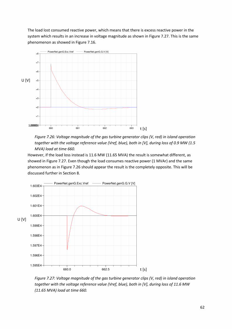
62
The load lost consumed reactive power, which means that there is excess reactive power in the
system which results in an increase in voltage magnitude as shown in Figure 7.27. This is the same
phenomenon as showed in Figure 7.16.
Figure 7.26: Voltage magnitude of the gas turbine generator clips (V, red) in island operation
together with the voltage reference value (Vref, blue), both in [V], during loss of 0.9 MW (1.5
MVA) load at time 660.
However, if the load loss instead is 11.6 MW (11.65 MVA) the result is somewhat different, as
showed in Figure 7.27. Even though the load consumes reactive power (1 MVAr) and the same
phenomenon as in Figure 7.26 should appear the result is the completely opposite. This will be
discussed further in Section 8.
Figure 7.27: Voltage magnitude of the gas turbine generator clips (V, red) in island operation
together with the voltage reference value (Vref, blue), both in [V], during loss of 11.6 MW
(11.65 MVA) load at time 660.
660 661 662 663
1.5998E4
+1
+2
+3
+4
+5
+6
+7
+8PowerNet.genG.Exc.Vref PowerNet.genG.G.V [V]
660.0 662.5
1.595E4
1.596E4
1.597E4
1.598E4
1.599E4
1.600E4
1.601E4
1.602E4
1.603E4PowerNet.genG.Exc.Vref PowerNet.genG.G.V [V]
t [s]
t [s]
U [V]
U [V]

63
7.2.6 Synchronisation of the power plant to the external power grid
In order to reconnect the power plant to the external power grid the synchronisation system of the
gas turbine generator has to be used as explained in Section 6.1.4. The same parameter settings as in
Section 7.2.1 are used, and the steam turbine generator is still off. The synchronisation is started by
closing the net breaker.
The gas turbine generator has to be in frequency and voltage regulation mode in order for the
synchronisation to occur. When the synchronisation is done the gas turbine changes its control
strategy to active and reactive power control, and the active power production reference value is
changed to rated power again. The transformer of the gas turbine generator changes back to
automatic tap changing.
Figure 7.28 shows the frequency of the gas turbine generator during synchronisation. When the net
breaker closes at time 803 the characteristic oscillation occur again. At time 780 the frequency makes
a dip, which is due to the synchronisation system which is trying to adjust the power system
frequency and voltage level in order to fulfil the synchronisation requirements at the net breaker.
The change in frequency occurring around time 845 is due to the change in power production, seen
in Figure 7.29.
Figure 7.28: Electrical frequency [Hz] of the gas turbine generator in island operation and
synchronisation back to normal operation at time 803. The disturbance around 780 is due to
adjustments during synchronisation, and the disturbance around 845 due to change of active
power.
Figure 7.29 shows the active and reactive power production by the gas turbine generator at the same
time, where the same characteristic oscillation occurs for both the active and reactive power. What
happens is basically the same as during the start-up explained in Section 7.2.1. As is further seen in
the figure is that the active power production is first oscillating around a value higher than the
reference value, and is after that slowly decreasing towards the reference value. This is because
when the power plant is connected to the external power grid the power production is higher than
the reference value and the gas turbine generator has to maintain the correct frequency. However,
around time 815 the generator changes to active power control and does therefore produce power
according to the reference value.
720 760 800 840 880 920
49.75
49.80
49.85
49.90
49.95
50.00
50.05
50.10
50.15
50.20
50.25
[Hz]
PowerNet.genG.f
t [s]
f [Hz]

64
Figure 7.29: Active power (P_out, blue) and reactive power (Q_out, green) produced by the
gas turbine generator in [W] an [VAr] respectively, together with the active power reference
value (P_ref, red) when synchronising back to normal operation from island operation at time
803. Around time 845 the generator change over to reactive power control simultaneously as
the active power reference value is changed.
After the power production of the gas turbine generator has been increased the steam turbine
generator can be started in the same way as explained in Section 7.2.1.
760 800 840 880 920 960 1000
-5.0E7
0.0E0
5.0E7
1.0E8
1.5E8
2.0E8
2.5E8
3.0E8
3.5E8PowerNet.genG.G.P_out PowerNet.genG.Gov.P_ref PowerNet.genG.G.Q_out
t [s]
P [W] Q [Var]
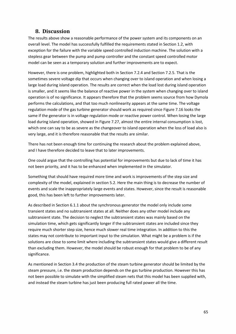
65
8. Discussion The results above show a reasonable performance of the power system and its components on an
overall level. The model has successfully fulfilled the requirements stated in Section 1.2, with
exception for the failure with the variable speed controlled induction machine. The solution with a
stepless gear between the pump and pump controller and the constant speed controlled motor
model can be seen as a temporary solution and further improvements are to expect.
However, there is one problem, highlighted both in Section 7.2.4 and Section 7.2.5. That is the
sometimes severe voltage dip that occurs when changing over to island operation and when losing a
large load during island operation. The results are correct when the load lost during island operation
is smaller, and it seems like the balance of reactive power in the system when changing over to island
operation is of no significance. It appears therefore that the problem seems source from how Dymola
performs the calculations, and that too much nonlinearity appears at the same time. The voltage
regulation mode of the gas turbine generator should work as required since Figure 7.16 looks the
same if the generator is in voltage regulation mode or reactive power control. When losing the large
load during island operation, showed in Figure 7.27, almost the entire internal consumption is lost,
which one can say to be as severe as the changeover to island operation when the loss of load also is
very large, and it is therefore reasonable that the results are similar.
There has not been enough time for continuing the research about the problem explained above,
and I have therefore decided to leave that to later improvements.
One could argue that the controlling has potential for improvements but due to lack of time it has
not been priority, and it has to be enhanced when implemented in the simulator.
Something that should have required more time and work is improvements of the step size and
complexity of the model, explained in section 5.2. Here the main thing is to decrease the number of
events and scale the inappropriately large events and states. However, since the result is reasonable
good, this has been left to further improvements later.
As described in Section 6.1.1 about the synchronous generator the model only include some
transient states and no subtransient states at all. Neither does any other model include any
subtransient state. The decision to neglect the subtransient states was mainly based on the
simulation time, which gets significantly longer if the subtransient states are included since they
require much shorter step size, hence much slower real time integration. In addition to this the
states may not contribute to important input to the simulation. What might be a problem is if the
solutions are close to some limit where including the subtransient states would give a different result
than excluding them. However, the model should be robust enough for that problem to be of any
significance.
As mentioned in Section 3.4 the production of the steam turbine generator should be limited by the
steam pressure, i.e. the steam production depends on the gas turbine production. However this has
not been possible to simulate with the simplified steam nets that this model has been supplied with,
and instead the steam turbine has just been producing full rated power all the time.

66
The solution of having very large or very small resistances to represent breakers in the system is a
fairly good approximation, but not ideal. This might contribute to some leakage of current and
power, but should not be a significant problem since the order of magnitude is a few amperes.
A similar problem is the phenomenon visible in Figure 7.17, i.e. that the frequency of the steam
turbine stays just below 50 Hz even though the generator is turned off. As mentioned in Section 7.2.4
this is probably due to a too small mechanical friction in combination with a leakage flow through the
valve connected to the turbine. The only thing that happens if the mechanical friction factor
increases is that the steady state value for the frequency decreases. Another thing that could be
source of the problem is the signal from the turbine governor. In order to decrease the frequency of
the generator, the control signal has to decrease. However, when the generator is turned off the
control signal from the governor is zero, and the frequency reaches equilibrium where the governor
cannot adjust further. The equilibrium point is then dependent on the friction and the leakage of
torque.

67
9. Conclusions and further research
9.1 Conclusions
The purpose of this project was to develop a model for an electrical system in a combined cycle
power plant as part of a simulator for power plant operators developed at Solvina AB. The modelling
has been performed in the modelling program Dymola, version 6.1.
The objectives was to derive a general, flexible model which can perform (at least) real time
simulations, and be able to simulate cold start of the system, normal load changes, trip of a
generator, and controlled change-over to island operation with resynchronisation.
The objectives have been fulfilled with mostly reasonable results. However, there are some results
where the behaviour of the system has not been considered reasonable. When the system is
exposed to very large load changes, like when changing-over to island operation, the system has
experienced a large undervoltage transient, regardless how the reactive power balance in the system
have been. The most likely reason for this is the calculations performed by Dymola, i.e. that it is
unable to handle to large changes at the same time. This problem has been left for further
improvements due to lack of time.
Another objective that has not been reached during the project is the development of a variable
speed regulated induction motor. A model has been compiled, but it has not been possible to make it
work in Dymola due to lack of enough knowledge about how the calculations are performed. Also
this problem has been left for further improvements due to lack of time.
The flexibility of the model is rather high and the model can therefore easily be adjusted to other
purposes and specific power plants.
The simulations are possible to perform in real time, but not with desirable long step size. In order to
achieve this more time has to be put on scaling and decreasing number of events.
9.2 Further research and possible improvements
There are some features of the power system that are desirable in the future but not included in this
version mainly due to lack of time. One major property is the unrealistic behaviour of the system
during a large loss of load, like during change-over to island operation. The large under voltage
transient that occurs needs to be handled to obtain a reasonable behaviour of the simulator.
Another important thing is to have a functional variable speed controlled induction motor model.
Here the problem has mainly been lack of time, but also lack of knowledge about how Dymola
perform the calculations.
Another feature which the system for the moment does not have is the possibility of performing the
synchronisation manually. This might be desirable if the model should be a part of a trainer for
operators where it could be pedagogical to make the synchronisations manually in order to fully
understand the control system and all the requirements for synchronisation.
Further, it could be desirable to include more and other types of protection systems, if it does not
affect the simulation time significantly. The protection devices included in this version are mainly due
to show their working principles.

68
As one of the requirements stated in Section 1.2 the model has the possibility to perform a cold start,
i.e. a start-up with the external power grid connected to the power plant. However, the model
cannot perform a black start, i.e. to start-up the power plant without being connected to the external
power grid. This is due to lack of external or extra power source to supply the field windings in the
generators. This might be a desirable feature to include in the future.

69
10. References [1] Svenska Kraftnät. (2003, November 4). Rapport om elavbrottet 23 september - Svenska kraftnät.
Retrieved October 5, 2010, from Svenska kraftnät: www.svk.se
[2] Omanovic, A. (2005). Dynamisk modellering av elkraftsystem. Göteborg: Chalmers University of
Technology.
[3] Eromon, D. (2006). Voltage Regulation Making use of Distributed Energy Resources (DER). 6 (2).
[4] Knazkins, V. (2004). Stability of Power Systems with Large Amounts of Distributed Generation.
Stockholm: KTH Institution för Elektroniska System.
[5] Stenborg, B. (1997). Elkraftsystem Del 1 - Systemet och dess lugndriftstillstånd. Göteborg: Gothia
Power AB.
[6] Saccomanno, F. (2003). Electric Power Systems - Analysis and Control. Surrey, British Columbia:
John Wiley & Sons.
[7] Kundur, P. (1993). Power system stability and control. Powertech Labs Inc., Surrey, British
Columbia: McGraw-Hill, Inc.
[8] Solvina AB. (2009). Elkraftdynamik på Södra Cell Mörrum. Göteborg: Solvina AB.
[9] Lundin, U. (2009). Regulation and dynamics. Elektricitetslära, Uppsala Universitet . Uppsala:
Elektricitetslära, Uppsala Universitet.
[10] Weedy, B., & Cory, B. (2005). Electric Power Systems, 4th ed. Southampton and London: Wiley
and Sons.
[11] Edwards, J. (2009). Electrical Machines - Course Notes. Brighton: University of Sussex.
[12] Larsson, M. (2000). Coordinated Voltage Control in Electric Power Systems, Doctoral dissertation.
Lund: Universitetstryckeriet.
[13] Getson, D. (2002, November 6). ABB De-energised Tap changers. Retrieved September 20, 2010,
from ABB i Sverige: http://search-ext.abb.com/library/Download.aspx?DocumentID=de-
energized_tap.pdf&LanguageCode=en&DocumentPartId=&Action=Launch
[14] Schlabbach, J. R.-H. (2008). Power System Engineering. Weinheim, Germany: Wiley-VCH.
[15] Russell Mason, C. (2010). The Art & Science of Protective Relaying. United States.
[16] Association, T. E. (1995). Power System Protection, Volume 2: System and methods. London, UK.
[17] Svenska Kraftnät. (2010, May 5). Svenska kraftnät. (Svenska kraftnät) Retrieved October 5, 2010,
from Svenska kraftnät: www.svk.se
[18] Association, M. (2010, Mars 24). http://www.modelica.org/. Retrieved Maj 25, 2010, from
Modelica® - A Unified Object-Oriented Language for Physical Systems Modeling, Language
Specification, Version 3.2: http://www.modelica.org/documents/ModelicaSpec32.pdf

70
[19] Vattenfall. (2010, April 28). Välkommen till vår anläggning i Uppsala. (Vattenfall AB) Retrieved
Juni 3, 2010, from Fjärrvärme och fjärrkyla, Vattenfall:
http://www.vattenfall.se/sv/uppsala_85772.htm
[20] Åkerman, M. (2010, Maj 27). Intervju Kraftvärmeverket Uppsala. Uppsala.
[21] Edvall, M. (2004). Beslutsunderlag ödrift. Göteborg: Solvina AB.
[22] Olesen, V. (2010, Oktober 12). Intervju. Göteborg.
[23] Johansson, B. (2010, Juni 8). Intervju. Göteborg.
[24] Arrillaga, J., & Watson, N. (2001). Computer modelling of electrical power systems (Vol. 2nd).
University of Canterbury, Christchurch, New Zealand: John Wiley & Sons, Ltd.
[25] Machowski, J., Bialek, J., & Bumby, J. (1997). Power System Dynamics and Stability. London: John
Wiley & Sons.
[26] Singhavilai, T., Anaya-Lara, O., & Lo, K. (2009). Identification of the Dynamic Equivalent of a
Power System. Universities Power Engineering Conference (UPEC), 2009 Proceedings of the 44th
International. Glasgow: Department of Electronic and Electrical Engineering, Strathclyde University.
[27] Kuphaldt, T. (n.d.). Wound Rotor Induction Motors. Retrieved September 2, 2010, from All About
Circuits: http://www.allaboutcircuits.com/vol_2/chpt_13/8.html
[28] Getson, D. (2002, November 6). ABB On-load tap changers (OLTC). Retrieved September 20,
2010, from ABB i Sverige: http://search-
ext.abb.com/library/Download.aspx?DocumentID=030129_On-
load.pdf&%20LanguageCode=en&DocumentPartId=&Action=Launch