Modelling Lateral Stability of Prefabricated Concrete ...kth.diva-portal.org/smash/get/diva2:940461/FULLTEXT01.pdfModelling Lateral Stability of Prefabricated Concrete Structures Caroline

Modelling Lateral Stability of PrefabricatedConcrete Structures

Caroline LindwallJonas Wester

TRITA-BKN. Master Thesis 490, Concrete Structures, June 2016ISSN 1103-4297,ISRN KTH/BKN/EX–490–SE

c©Lindwall, Wester 2016Royal Institute of Technology (KTH)Department of Civil and Architectural EngineeringDivision of Concrete StructuresStockholm, Sweden, 2016

Abstract

Stability calculations of prefabricated concrete structures with help of FEM-tools demandknowledge about how the elements are related to each other. This thesis concerns howjoints between building elements affect the results when modelling prefabricated concretestructures, with demarcation to joints between hollow core (HC) slabs and between solidwall elements. The thesis also covers how the properties of the floor can be adjusted toaccount for the effects of the joints without modelling every single element.

The work started by measuring the deflection of 10 HC-slabs jointed together and loadedin-plane acting as a deep beam, in a FE-model made with RobotTM from Autodeskr. Thejoints between the HC-elements were modelled either rigid or elastic, and the cross-sectionand the length of the HC-elements were varied. The linear elastic stiffness between theHC-elements was obtained from the literature as 0.05 (GN/m)/m. The results showed thata changed cross-section geometry gave greater differences in deformation than a changedlength. The in-plane shear modulus was then adjusted for the HC-elements in the rigidcases until the same deflection was achieved as for the elastic cases. The result showedthat the shear modulus in average for the different cross-section geometries and lengthshad to be reduced with a factor of 0.1 to account for the joints.

Based on the geometry of a castellated joint between prefabricated solid concrete walls, acalculation model was developed for its linear elastic stiffness. The result was a stiffness of1.86 (GN/m)/m. To verify the calculated stiffness, a FE-model was developed consistingof a 30m high wall, loaded horizontally in-plane and with one or two vertical joints wherethe stiffness was applied. The deflection and the reaction forces were noted and the resultfrom the calculated stiffness was compared to other stiffnesses and assessed reasonable.The reaction forces were shown to depend on the stiffness of the joint.

The reduced in-plane shear modulus of the HC-elements and the calculated stiffness of thewall joints were then used in a FE-model of a 10-storey building stabilised by two units.The vertical reaction forces were analysed and the results showed 0.02% difference in thereaction forces in the stabilising units when consideration of the joints between the HC-elements were taken into account and 0.09% when the vertical joints in the shear wall weretaken into account. The results for the wall joint differed from the results when only thewall was modelled. This was thought to be a result of that the floors counteract the sheardeformations in the wall joints. The influence of the floor joints was not significant for thebuilding considered in this thesis, but for buildings with non-continuous configuration ofthe stiffness in the shear walls the outcome may be another, in these cases the reductionfactor may be useful.

i

Sammanfattning

Vid stabilitetsberäkningar av prefabricerade betongstommar med hjälp av FEM-verktygställs krav på kunskap om hur elementen förhåller sig till varandra. Detta arbete berörhur fogar mellan byggnadselement påverkar modellering av prefabricerade betongstommarmed avgränsning till fogar mellan håldäckselement och mellan solida väggelement. Arbetetberör även en studie i hur ett bjälklags egenskaper kan justeras så att fogarnas effekt kantillvaratas utan att modellera varje enskilt håldäckselement.

Arbetet inleddes med att utböjningen analyserades hos 10 st ihopskarvade håldäcksele-ment, lastade i dess plan likt en hög balk, i en FE-modell skapad i programmet RobotTM

från Autodeskr. Fogarna mellan håldäcken modellerades som antingen rigida eller elastiskaoch håldäckens tvärsnittsgeometri och längd varierades under testet. Den linjära styvhetenmellan håldäcken togs från litteraturen som 0.05 (GN/m)/m. Resultatet visade att ändradtvärsnittsgeometri gav större skillnader för deformationen än varierad längd på håldäcken.Håldäckens skjuvmodul justerades sedan i dess plan för de rigida testen tills dess att deuppnådde samma utböjning som de elastiska. Resultatet visade att skjuvmodulen be-hövdes reduceras med en faktor 0.1, i medeltal för de olika tvärsnittsgeometrierna ochhåldäckslängderna.

Utefter geometrin på en fog med förtagningar mellan prefabricerade väggar togs en beräkn-ingsmodell fram för den linjärelastiska styvheten i väggfogarna. Resultatet blev en styvhetpå 1.86 (GN/m)/m. För att verifiera den beräknade styvheten togs en FE-modell frambestående av en 30m hög vägg lastad horisontellt i dess plan med en eller två vertikala fogardär en linjär styvhet applicerades. Utböjningen samt reaktionskrafterna noterades, resul-tatet för den uträknade linjära styvheten jämfördes med andra styvheter och bedömdesutifrån detta vara rimlig. Reaktionskrafterna visade sig vara beroende av styvheten påfogen.

Den sänkta skjuvmodulen för håldäcken och den beräknade linjära elasticiteten för väg-garna användes sedan i en FE-modell av en 10-våningsbyggnad med två stabiliserandeenheter där de vertikala reaktionskrafterna analyserades. Resultatet visade att endast0.02 procentenheter skiljer reaktionskrafterna i de stabiliserande enheterna då hänsyn tastill fogarna mellan håldäcken och 0.09 procentenheter då hänsyn tas till fogarna mellanväggarna. Resultatet skiljer sig från när endast väggen modellerades, vilket tros bero påatt bjälklaget hjälper till att motverka deformationer i väggfogarna. Fogen mellan bjälk-lagselementen tros kunna ha större inverkan på en byggnad med stabiliserande enhetersom drastiskt ändrar styvhet från ett plan till ett annat, i dessa fall kan den framtagnareduktionsfaktorn vara av nytta.

iii

Preface

This master thesis is the final work of our Degree of Master at the Department ofCivil and Architectural Engineering at KTH Royal Institute of Technology. Thework has been carried out at Tyréns AB during the spring semester of 2016.

A special thanks is expressed to our supervisor, Adjunct Professor Mikael Hallgren,for advising and guiding us through out all the work of this thesis and to Nils Ekrothat Tyréns AB, for valuable insights in precast concrete structures and for introducingus to the subject of this thesis.

We are also grateful to Ebrahim Zamani at Tyréns AB for his advices and assistancein the FE-program RobotTM, Bo Westerberg for his experience and advices, KlaraBergman and Ludvig Bergström Björn for their contribution to the editing workand last but not least we thank our examiner, Professor Anders Ansell.

Stockholm, June 2016

Jonas Wester & Caroline Lindwall

v

Notations

A Area m2

a0 Void width in HC-slabs ma1 Centre distance between voids in HC-slabs mB Width m[B] Strain-displacement matrixb Width m[D] Constitutive /membrane stiffness matrix{D} Displacement vector md Depth mE Young’s modulus PaEd Design value of effect of actions −Ekg Young’s modulus in kg/cm2, kg: kilogram-force kg/cm2

F Force kNFk Area of interface of shear key joints cm2

fc Concrete strength Pafy Yield strength of steel PaG Shear modulus PaH Height m[H] Shear stiffness matrixh Height mhc Height to centre of void in HC-slabs mh0 Void height in HC-slabs mh1 Height of upper flange in HC-slabs mh2 Height of lower flange in HC-slabs mI Moment of inertia m4

[K] Global stiffness matrix / Bending stiffness matrixk Stiffness kN/m[k] Local stiffness matrixL Length mM Moment kNmN Normal force kNP Load kNPcr Cracking load kNPu Ultimate load kNq Line load kN/m{R} Reaction force vector kNRd Design value of resistance −

vii

V Shear force kN

α Angle of compressive strut radδ Deflection mε Strain −γ Self-weight kN/m3

γ/γxy Shear angle radλ Reduction factor −ν Poisson’s ratio −σ Stress Paτ Shear stress Pa

viii

Abbreviations

3D Three DimensionsDOF Degrees of FreedomDSC Discontinuity ElementFE Finite ElementFEM Finite Element MethodEQU EquilibriumHC Hollow CoreSTR StrengthULS Ultimate Limit State

ix

Contents

Abstract i

Sammanfattning iii

Preface v

Notations vii

Abbreviations ix

1 Introduction 1

1.1 Background . . . . . . . . . . . . . . . . . . . . . . . . . . . . . . . . 1

1.2 Challenges . . . . . . . . . . . . . . . . . . . . . . . . . . . . . . . . . 2

1.2.1 Hollow core slabs . . . . . . . . . . . . . . . . . . . . . . . . . 2

1.2.2 Shear walls . . . . . . . . . . . . . . . . . . . . . . . . . . . . 2

1.3 Aim and scope . . . . . . . . . . . . . . . . . . . . . . . . . . . . . . 2

1.4 Limitations . . . . . . . . . . . . . . . . . . . . . . . . . . . . . . . . 3

2 Structural stability 5

2.1 Actions on buildings . . . . . . . . . . . . . . . . . . . . . . . . . . . 5

2.1.1 Horizontal loads . . . . . . . . . . . . . . . . . . . . . . . . . . 6

2.1.2 Vertical loads . . . . . . . . . . . . . . . . . . . . . . . . . . . 7

2.2 Stabilising shear walls and cores . . . . . . . . . . . . . . . . . . . . . 7

2.2.1 Arrangement of stabilising members . . . . . . . . . . . . . . . 8

2.3 Distribution of lateral forces . . . . . . . . . . . . . . . . . . . . . . . 8

2.3.1 Deep beams . . . . . . . . . . . . . . . . . . . . . . . . . . . . 9

xi

2.3.2 Load distribution to shear walls . . . . . . . . . . . . . . . . . 10

3 Precast concrete structures 11

3.1 General . . . . . . . . . . . . . . . . . . . . . . . . . . . . . . . . . . 11

3.2 Hollow core slabs . . . . . . . . . . . . . . . . . . . . . . . . . . . . . 11

3.2.1 Floor diaphragm action . . . . . . . . . . . . . . . . . . . . . . 12

3.3 Precast walls . . . . . . . . . . . . . . . . . . . . . . . . . . . . . . . 13

3.3.1 Shear wall behaviour . . . . . . . . . . . . . . . . . . . . . . . 14

3.4 Connections . . . . . . . . . . . . . . . . . . . . . . . . . . . . . . . . 16

3.4.1 Shear key joints . . . . . . . . . . . . . . . . . . . . . . . . . . 16

3.4.2 Joints between hollow core slabs . . . . . . . . . . . . . . . . . 18

3.4.3 Ties . . . . . . . . . . . . . . . . . . . . . . . . . . . . . . . . 20

4 Finite element method 21

4.1 Finite element method - theory . . . . . . . . . . . . . . . . . . . . . 21

4.1.1 Plane stress theory . . . . . . . . . . . . . . . . . . . . . . . . 22

4.1.2 Plate theory . . . . . . . . . . . . . . . . . . . . . . . . . . . . 23

4.1.3 Shell elements . . . . . . . . . . . . . . . . . . . . . . . . . . . 23

4.1.4 Nonlinear analysis . . . . . . . . . . . . . . . . . . . . . . . . 24

4.2 Modelling with RobotTM . . . . . . . . . . . . . . . . . . . . . . . . . 24

4.2.1 Predefined hollow core slabs & user-defined panels . . . . . . . 24

4.2.2 Mesh . . . . . . . . . . . . . . . . . . . . . . . . . . . . . . . . 26

4.2.3 Load . . . . . . . . . . . . . . . . . . . . . . . . . . . . . . . . 27

4.2.4 Releases . . . . . . . . . . . . . . . . . . . . . . . . . . . . . . 27

4.2.5 Solvers for static analysis . . . . . . . . . . . . . . . . . . . . . 28

4.2.6 Nonlinear static analysis in RobotTM . . . . . . . . . . . . . . 29

5 Models used in the analyses 31

5.1 Floor joints . . . . . . . . . . . . . . . . . . . . . . . . . . . . . . . . 31

5.1.1 Floor model . . . . . . . . . . . . . . . . . . . . . . . . . . . . 31

5.1.2 Verification with hand calculation . . . . . . . . . . . . . . . . 37

xii

5.2 Shear key joints . . . . . . . . . . . . . . . . . . . . . . . . . . . . . . 40

5.2.1 Estimation of shear key stiffness . . . . . . . . . . . . . . . . . 41

5.2.2 Wall model . . . . . . . . . . . . . . . . . . . . . . . . . . . . 42

5.3 Building model . . . . . . . . . . . . . . . . . . . . . . . . . . . . . . 45

5.3.1 General model settings . . . . . . . . . . . . . . . . . . . . . . 47

5.3.2 Floor joint settings . . . . . . . . . . . . . . . . . . . . . . . . 48

5.3.3 Wall joint settings . . . . . . . . . . . . . . . . . . . . . . . . 49

6 Results from the analyses 51

6.1 Behaviour of floor model . . . . . . . . . . . . . . . . . . . . . . . . . 51

6.1.1 Deflections, FE-simulations . . . . . . . . . . . . . . . . . . . 51

6.1.2 Deflections, Hand calculations . . . . . . . . . . . . . . . . . . 52

6.1.3 Reduction factor . . . . . . . . . . . . . . . . . . . . . . . . . 54

6.2 Behaviour of wall model . . . . . . . . . . . . . . . . . . . . . . . . . 55

6.3 Behaviour of building model . . . . . . . . . . . . . . . . . . . . . . . 60

6.3.1 Influence of floor joints . . . . . . . . . . . . . . . . . . . . . . 60

6.3.2 Influence of wall joints . . . . . . . . . . . . . . . . . . . . . . 62

6.3.3 Combination of floor joints and wall joints . . . . . . . . . . . 67

7 Discussion 69

7.1 RobotTM models . . . . . . . . . . . . . . . . . . . . . . . . . . . . . . 69

7.2 Floor joints . . . . . . . . . . . . . . . . . . . . . . . . . . . . . . . . 70

7.2.1 Floor joints in the building model . . . . . . . . . . . . . . . . 70

7.3 Wall joints . . . . . . . . . . . . . . . . . . . . . . . . . . . . . . . . . 71

7.3.1 Shear key joints in the building model . . . . . . . . . . . . . 71

7.4 Hotel Hagaplan . . . . . . . . . . . . . . . . . . . . . . . . . . . . . . 72

7.5 Conclusions . . . . . . . . . . . . . . . . . . . . . . . . . . . . . . . . 72

7.6 Further research . . . . . . . . . . . . . . . . . . . . . . . . . . . . . . 73

Bibliography 75

xiii

Appendix A - Comparison between the two models 79

Appendix B - Drawings of the building model 85

Appendix C - Calculations 87

xiv

Chapter 1

Introduction

More and more engineers make use of finite element method (FEM) software in thedesign process of buildings. As these models can become large and complicated itis of great importance that the engineer possess the knowledge of how to use andinterpret the models of these programs.

1.1 Background

The subject of this thesis arose from a real case, where two computational modelsof a hotel building were made, by two different companies, using the FEM softwareAutodesk R© RobotTM Structural Analysis. The building is called Hotel Hagaplanand provides the basis for this thesis. The two models gave different results withrespect to load distribution between the walls and columns. A design consultantcompany (Company A) was hired to make an early stage estimation of the loadson the foundation. A 3D model of the building was built up in RobotTM basedon the preliminary design of the building. The model will be referred to as modelA. The purpose of model A was to check the structural stability and the load dis-tribution. The second model, model B was created by a company specialised inprecast concrete (Company B). This model was to be used as the basis for designof the precast concrete elements and their connections. During the planning of thedesign of the foundation it was discovered that model A had provided much lowerforces in the stabilising units i.e. the walls, than model B. The results from modelA indicated that the building was stabilised against overturning by its own weight,while model B indicated that the building required anchorage. The fact that thetwo models provided different results gave rise to an insecurity in the loads for whichthe foundation was to be designed.

A normal procedure for the design of precast concrete structures is to first makeestimations on load distribution and structural stability based on the preliminarydesign of the building. Further on in the process the final design of the precastconcrete elements is made by the manufacturer.

1

CHAPTER 1. INTRODUCTION

1.2 Challenges

In the earlier stages of a project, details and solutions are usually not finally decideddue to that a certain level of changes still are possible. However, some investigationsand information are still needed to make decisions and develop a project further.Receiving approximate information in a short time is usually preferred over exactinformation, based on data that might be changed in the continuing process. Trust-worthy information and precision in calculations is still valuable and if there is away to reach it within the demand of the early stages, time and money can be saved.

When modelling precast concrete structures with FEM, the real structure has to besimplified to fit into the FE-model, and further assumptions and simplifications aremade with respect to the amount of time for modelling and computation. Detailsin the structure may need to be estimated into simpler designs in order to save timeif the details are assumed to affect the desired result in a small scale.

1.2.1 Hollow core slabs

Hollow core slabs are produced in a shape to make them movable with cranes andtrucks and then cast together with longitudinal joints. A fast way to model a hollowcore slab floor is to neglect the joints and assume that the joints will not influencethe behaviour in the FE-analysis, but in reality the stiffness of the floors will beaffected by the joints. It would be advantageous to not have to model each HC-element individually but to model the floor in one piece and also take the effect fromthe longitudinal joints into account at the same time.

1.2.2 Shear walls

The joints in the shear walls will have other strength and stiffness properties thanthose of the wall itself. The stress distribution in the walls will thus depend on thestiffness of the joints (Olesen, 1975).

1.3 Aim and scope

The general aim of this thesis is to develop recommendations on how to modelprecast concrete buildings with sufficient reliability with respect to the behaviourof the building regarding load distribution and stability. The modelling suggestionsshould be compatible with investigations in an early stage in a project where timeand simplicity are major priorities. The investigation concerns how special featuresof precast concrete structures such as the connections, influence the total stiffnessand behaviour of the structure and how they can be accounted for in the FE-modelswithout being modelled explicitly.

2

1.4. LIMITATIONS

The two models of the hotel building Hotel Hagaplan were compared and investi-gated in a pre-study, which is presented in Appendix A.

Background theory about structural stability, precast concrete structures and theirconnections and FEM was obtained in a literature study.

A series of numerical tests was set up to study the influence of longitudinal jointsbetween hollow core elements subjected to horizontal loading. In the test series ahollow core slab floor was modelled with elastic and completely rigid joints respec-tively. A reduction factor, which gives an equivalent stiffness for a floor modelledwithout joints, was calculated. The floor was modelled with different length andthickness to provide information on the variation of the results.

An other numerical test was performed to investigate the influence of vertical shearkey connections between precast concrete wall elements. Different degrees of stiffnessof the connection were applied and evaluated in a FE-model of a wall subjected tohorizontal loading.

The joints influence on load distribution in a structure were studied in an FE-modelof a 10-storey building.

1.4 Limitations

Hotel Hagaplan was used to demarcate the type of building that was studied. HotelHagaplan is a building of precast concrete with a load bearing system of columnsand stabilising shear walls/cores. The floor constitutes of hollow core slabs and theshear walls are generally connected with vertical shear keys. The investigations ofthe joints were limited to treat their influence on the in-plane behaviour regardingtheir stiffness. The focus of investigation was placed on longitudinal joints betweenthe hollow core elements and vertical shear key joints between the wall elements.Other connections were simplified as rigid or pinned in the models. The stress levelsor strength properties of the joints were not treated.

The dynamic effects of the wind was neglected and all simulations were performed asstatic. All materials were assumed to be linear elastic. Settlements in the foundationwere not taken into account in the analysis. The effects of structural topping on thehollow core slabs were not considered. More limitations and demarcations will bepresented further in the text.

3

Chapter 2

Structural stability

This chapter provides basic background information about the actions relevant forstability checks of buildings. The typical stabilising system for precast residentialand office buildings consisting of shear walls and cores is described.

2.1 Actions on buildings

Different kinds of actions are considered when the structural stability of a building ischecked. The actions are divided in permanent actions, such as self-weight from thestructures or weight from permanently mounted equipment, variable actions suchas actions from wind, snow or imposed loads on floors, and accidental actions fromexplosions and impact from vehicles.

According to SS-EN 1990 (2010), four different types of ultimate limit states are tobe checked (if relevant) where the loads are combined into cases and considered asfavourable or unfavourable by multiplying with different coefficients.

In this thesis the states which treat deformations in the ground and fatigue inmaterials will not be further described or treated. Left is:

1. EQU - "Loss of static equilibrium of the structure or any part of it consideredas a rigid body..."(SS-EN 1990, 2010). EQU is verified by the criteria inequation (2.1) below where Ed,dst represents the dimensioning destabilisingloads and Ed,stb represents the stabilising loads.

Ed,dst ≤ Ed,stb (2.1)

2. STR - "Internal failure or excessive deformation of the structure or structuralmembers..."(SS-EN 1990, 2010). STR is verified by the criteria in equation(2.2) below where Ed represents the design value of the effect of actions andRd is the corresponding design value of the resistance.

Ed ≤ Rd (2.2)

5

CHAPTER 2. STRUCTURAL STABILITY

EQU is in practice failure due to overturning or sliding of the building while STRtreats failure, or too big deformation in the structure or in individual components,see figure 2.1a) to 2.1d) below (Isaksson et al., 2010).

a) Overturning b) Sliding c) Internal stability d) Failure

Figure 2.1 Ultimate limit states in EQU (a and b) and STR (c and d).(Remakebased on Heyden et al. (2008)).

2.1.1 Horizontal loads

Wind load

Wind load on buildings has in general the greatest destabilising influence. It is acomplex phenomenon and difficult to approximate (Lorentsen et al., 2000). Thebuilding height, surrounding buildings, terrain and the shape of the structure aresome of the parameters influencing its behaviour (Mendis et al., 2007). Principallythe wind is a dynamic action, but since buildings normally have a high damping abil-ity and are insensitive to short dynamic actions, the wind load is usually consideredas an equivalent static action (Isaksson et al., 2010).

The wind load on a rectangular structure is often, in the Eurocodes, a case wherethe load acts as a pressuring and a suction field load on opposite sides. Wind mayalso cause overpressure on the façade elements from the inside and friction on theparallel façades. The force from the friction is depending on the façade material andthe overpressure is a result of leakage, often around windows and doors.

The overpressure inside is spread equally on the façades and is therefore not takeninto account in a stability calculation. The force from the friction can also beneglected if the façade area parallel to the wind direction is less than, or equal to, 4times the area perpendicular to the wind direction (SS-EN 1991-1-4:2005, 2008).

The wind pressure varies depending on the distance from the ground which must betaken into consideration when the wind action is applied to the building. In designaccording to the Eurocode, the building is divided in sections where the velocitypressure has different uniform magnitudes. A higher pressure is applied on thehigher parts of the building. The division into load sections is depending on theheight to width ratio h/b of the building.

6

2.2. STABILISING SHEAR WALLS AND CORES

A variation can also appear in the horizontal direction which causes a twisting of thebuilding. Symmetric buildings with only one stabilising core is particularly sensitiveto this phenomenon (SS-EN 1991-1-4:2005, 2008).

Sway imperfections

It must be taken into consideration when structures are designed that columnscan be mounted incorrectly. The axial force of an inclined column gives rise to ahorizontal load in the structure. Unintentional eccentricities in members are treatedby considering sway imperfections. In a structure with several columns, the swayimperfections are often accounted for as an overall load from all columns based onthe probability that they have an eccentricity. This overall load can be applied tothe building at each floor (Isaksson et al., 2010).

2.1.2 Vertical loads

The vertical loads on a building consist mainly of dead loads, imposed loads andsnow load. The stabilising action is provided by the vertical loads, but they alsogovern destabilising actions when second-order effects are considered.

2.2 Stabilising shear walls and cores

The choice of stabilising system should be done with respect to what is suitable forthe specific building. Type of occupancy, building height, construction method andsize of lateral loads in form of wind and seismic loads are some of the factors thathave influence on the choice of stabilising system. The lower part of buildings isusually used for occupancies that require large open spaces such as entrance hallsand shops, which demands for a conscious configuration of the stabilising system(Lorentsen et al., 2000).

The structural stability of a building can be achieved with frames, trusses, shearwalls, cores or with a combination of these (Lorentsen et al., 2000). In precast con-crete residential and office buildings the stability is usually ensured with stabilisingcores and shear walls (Bachmann and Steinle, 2011). Thus in this thesis stabilisingcores and shear walls will be treated.

In order to have a flexible building with respect to disposal of the premises, a systemof load bearing walls are commonly avoided in favour of a load bearing system ofcolumns. Structural stability for these buildings can be achieved by frame action bythe columns or with specific stability members such as cores or shear walls. Thesemembers are commonly placed to form elevator shafts and stairwells. Frame actionwith columns demands for a monolithic structure with rigid connections between thecolumns and the floor. For precast concrete structures these types of connections

7


are difficult to achieve why stability by frame action is not appropriate for precastconcrete structures (Lorentsen et al., 2000).

The precast concrete walls of a shear wall structure act as cantilever walls, carryingvertical loads and horizontal, in-plane forces (BCA, 2001). The horizontal forcesgive rise to moments and shear forces in the wall and the vertical load causes axialcompression, as shown in figure 2.2 (Park and Paulay, 1975).

Windpressure

Windsuction

CompressionTension

M

N

V

Figure 2.2 Stability with shear walls. The wall is subjected to shear force (V ),moment (M) and axial force (N). (Remake based on Elliott and Jolly(2013)).

2.2.1 Arrangement of stabilising members

For a building where the floor is considered completely rigid, three buckling modesare possible. These are translations in the two horizontal directions and rotationaround the vertical axis. This is often a legitimate simplification. The stabilisingmembers must be placed to resist these buckling modes (Lorentsen et al., 2000).If all stabilising walls are positioned parallel to each other there will be a lack ofstability in the perpendicular direction since only forces applied in the direction ofthe plane of the walls can be resisted. This means that the walls must be placed inat least two non-parallel directions to resist the translations (Bachmann and Steinle,2011). Furthermore, to limit rotation, at least three walls are required and thesemust be placed so that they do not intersect in the same vertical line. Still, onlyone core is not sufficient to restrain the rotation. Two cores or one core and a wallwith a large distance in between are usually required (Lorentsen et al., 2000).

2.3 Distribution of lateral forces

When it comes to structural stability of buildings, the floors have an importantrole of transferring collected lateral forces from wind and sway imperfections fromfaçades, walls and columns to the stabilising members (Westerberg, 1999). Thefloor slabs are usually considered as deep beams or diaphragms when transferring

8

2.3. DISTRIBUTION OF LATERAL FORCES

the lateral load due to their geometry. Figure 2.3 shows the principal path of windload, from application through the façade on the floor to the foundation.

Wind load

Figure 2.3 Principal load path of wind from floor edge to foundation.

2.3.1 Deep beams

According to the Eurocode, a beam with height equal to, or more than one thirdof the length i.e. h ≥ L/3 cannot be described by ordinary beam theory due todiscontinuities in stresses. Structures of this kind, with height and length of thesame order and a thickness which is normally much less, are considered as deepbeams or diaphragms when loaded in their own plane. The term deep beam isnormally used for diaphragms that act as beams on two or more supports. Thestress distribution in a deep beam differs from that of an ordinary beam. The stressdistribution in a deep beam will not be linear as in the case of an ordinary beam inthe uncracked state, due to the effects of shear forces. A deep beam is consideredto act as an arch with a tendon, see figure 2.4 (Ansell et al., 2014).

Tensile tendon

Compression arch

Figure 2.4 Arch with tendon. (Remake based on Ansell et al. (2014)).

9


2.3.2 Load distribution to shear walls

In what way the lateral load is distributed between the shear walls of a buildingdepends mainly on four factors. These are the properties of the supporting soil andfootings, the stiffness of the floor diaphragms, the relative stiffness between the wallsand of their connections, and the eccentricity of the application of the lateral loadswith respect to the centre of rigidity of the walls (PCI, 2007). When estimatingthe load distribution on the stabilising members of a structure by hand calculations,assumptions are usually made regarding the stiffness of the walls and floors. Thereare two common methods for determining the loads on the walls depending on thestiffness of the walls and the diaphragm and these are the tributary area approachand the relative stiffness approach.

Tributary area approach

The tributary area approach is used for flexible diaphragms where the shear wallscan be considered as completely rigid in relation to the floor which causes the lateralforces to be distributed between the shear walls according the tributary area (Ghoshand Fanella, 2003). This approach is analogous with conventional beam theory wherethe supports are considered as stiff.

Relative stiffness approach

For the relative stiffness approach the diaphragm is assumed to be completely rigidand the load on the shear walls will therefore be distributed according to the relativestiffness of the walls since these are forced to displace equally or proportional to theirdistance to the centre of rotation (Ghosh and Fanella, 2003).

The assumptions in the relative stiffness approach regarding the stiffness of floordiaphragms are investigated by Roper and Iding (1984) for buildings with irregularfeatures. According to their study the stiffness of the diaphragm has a very smalleffect on the load distribution between the shear walls when the floor plan has acomplex geometry provided that the walls have a uniform configuration. If, however,the walls contain a sudden change of stiffness from one floor to another, as in caseswith large openings or other changes in geometry, the load distribution on the wallswill be significantly influenced by the stiffness of the diaphragm.

10

Chapter 3

Precast concrete structures

This chapter covers the precast concrete elements relevant with respect to HotelHagaplan. The principal behaviour of the elements including their connections,when subjected to horizontal loads, are explained.

3.1 General

When designing buildings with precast concrete elements, a special considerationregarding the structural continuity must be taken, compared to when building castin-situ buildings where this condition is fulfilled as a natural result of the castingprocess. The structural continuity of precast buildings must be ensured when theelements are connected to each other (BCA, 2001).

3.2 Hollow core slabs

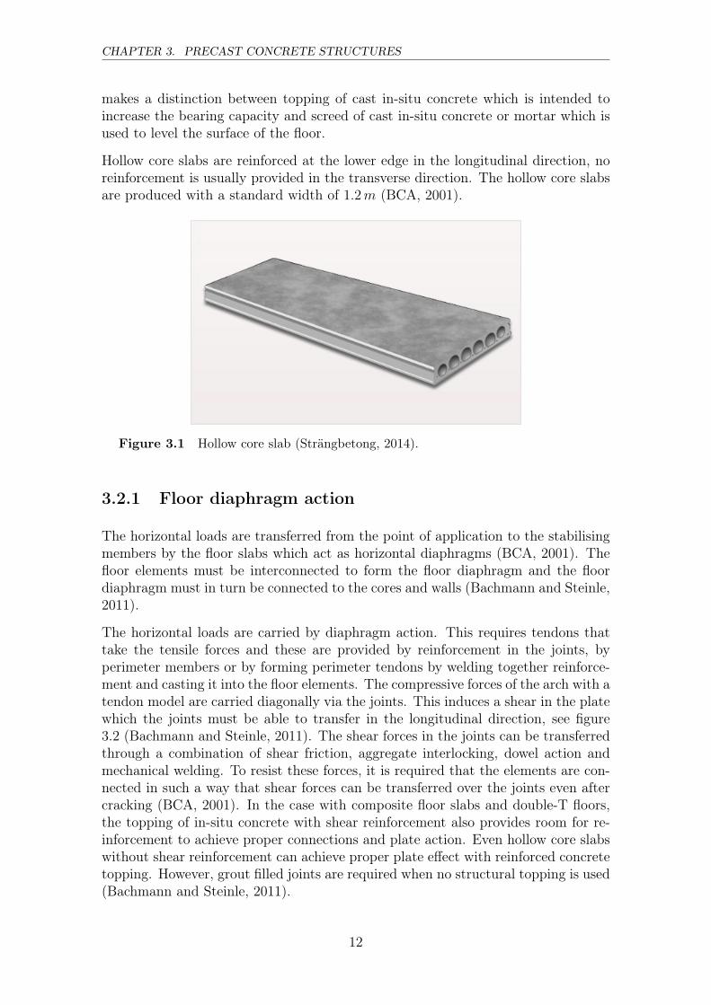
One of the most economic precast concrete floor systems is the precast hollow coreslab (figure 3.1). Up to 40% of the material can be saved compared to solid concrete(Bachmann and Steinle, 2011).

Hollow core elements are usually used in floors and roofs, but may also be usedin walls and other special applications. The methods used for manufacturing theelements are extrusion, slipforming and mouldcasting. The lateral edges of theelements have a grooved profile, this profile provides a shear key for the transferof the out-of-plane shear between the elements. In order for the slab to act as adiaphragm, the joints also must function as horizontal shear joints. This action canbe improved with vertical grooves in the joints (SS-EN 1168:2005+A3:2011, 2011).

According to SS-EN 1168:2005+A3:2011 (2011) a hollow core slab is a monolithicprestressed or reinforced element with constant overall depth. The element containslongitudinal voids with constant cross section. These voids are called cores and areformed by vertical webs and an upper and lower flange of concrete. The standard

11

CHAPTER 3. PRECAST CONCRETE STRUCTURES

makes a distinction between topping of cast in-situ concrete which is intended toincrease the bearing capacity and screed of cast in-situ concrete or mortar which isused to level the surface of the floor.

Hollow core slabs are reinforced at the lower edge in the longitudinal direction, noreinforcement is usually provided in the transverse direction. The hollow core slabsare produced with a standard width of 1.2m (BCA, 2001).

Figure 3.1 Hollow core slab (Strängbetong, 2014).

3.2.1 Floor diaphragm action

The horizontal loads are transferred from the point of application to the stabilisingmembers by the floor slabs which act as horizontal diaphragms (BCA, 2001). Thefloor elements must be interconnected to form the floor diaphragm and the floordiaphragm must in turn be connected to the cores and walls (Bachmann and Steinle,2011).

The horizontal loads are carried by diaphragm action. This requires tendons thattake the tensile forces and these are provided by reinforcement in the joints, byperimeter members or by forming perimeter tendons by welding together reinforce-ment and casting it into the floor elements. The compressive forces of the arch with atendon model are carried diagonally via the joints. This induces a shear in the platewhich the joints must be able to transfer in the longitudinal direction, see figure3.2 (Bachmann and Steinle, 2011). The shear forces in the joints can be transferredthrough a combination of shear friction, aggregate interlocking, dowel action andmechanical welding. To resist these forces, it is required that the elements are con-nected in such a way that shear forces can be transferred over the joints even aftercracking (BCA, 2001). In the case with composite floor slabs and double-T floors,the topping of in-situ concrete with shear reinforcement also provides room for re-inforcement to achieve proper connections and plate action. Even hollow core slabswithout shear reinforcement can achieve proper plate effect with reinforced concretetopping. However, grout filled joints are required when no structural topping is used(Bachmann and Steinle, 2011).

12

3.3. PRECAST WALLS

Tensile tendon

Compression arch

Shear wall

Figure 3.2 Diaphragm action with hollow core slabs. (Remake based on Elliottand Jolly (2013)).

Prestressing hollow core slabs can lead to a varying deformation between elementswhich can result in problems at the joints. When the slab is to be used as a di-aphragm there must be sufficient space in the joints. One way of ensuring thetransfer of in-plane loads is to partly fill and reinforce some particular voids. Thereinforcement act as dowels between the elements (Bachmann and Steinle, 2011).

Concrete diaphragms are commonly thought of as rigid when compared to the sta-bilising members. Depending on the load a hollow core diaphragm may need to beconsidered as a flexible diaphragm (Buettner and Becker, 1998).

3.3 Precast walls

Precast concrete walls are used both as façades and internal walls. There are severaltypes of precast concrete walls: sandwich walls, in-fill walls and shear walls are someexamples (PCI, 2007). This thesis will focus on solid, load bearing shear walls.

The size of the precast wall elements is limited by transportation factors. Cranes inthe factory and at the building site must manage the weight of the elements (BCA,2001). Furthermore, the dimensions of the elements must allow for transportationfrom the factory to the building site. The elements are typically of storey-height andup to four to nine meters wide. A thickness of 200− 400mm is common. The wallelements are typically cast in horizontal position in individual forms and providedwith conventional reinforcement (PCI, 2007). Profiled edges of the wall can beobtained which provide the shape of the joints when the elements are interconnected.

13


3.3.1 Shear wall behaviour

For precast concrete buildings, stabilising walls and cores can be constructed ofcast in-situ concrete or precast concrete elements. In case of the latter, storey-high precast wall elements are normally used (Bachmann and Steinle, 2011). Theseelements are connected by vertical and horizontal joints. When the wall is subjectedto horizontal loading, internal moments and shear develop, which in turn, causenormal and shear stresses in the vertical and horizontal intersections of the wall.Shear stresses appear in the joints not only due to horizontal loading but also incase of vertical non-uniform loading. If the components are to interact, shear jointsthat can transfer the forces are required. There are several methods to constructthe connections between wall elements. The castellated joint, i.e. shear key joint,with or without interlacing steel, is a popular approach to achieve shear transfer(BCA, 2001). Transverse reinforcement in the joint is designed to divide the shearforces into horizontal tension components and diagonal compression components, sothat the wall can act as a deep beam. This reinforcement can be concentrated tothe floor levels or distributed over the joint. The horizontal joints between the wallelements are mainly loaded in compression, then friction offers the transfer of shearforces (Bachmann and Steinle, 2011).

The precast concrete wall performs more or less as a homogeneous plate regardinghorizontal loads depending on the stiffness of the joints. With low stiffness in thejoints, the wall acts more as a series of beams and the stiffer the joints are, the morethe wall will behave as a homogeneous plate (BCA, 2001).

The stress distribution in the wall depends on the deformations. According to Olesen(1975) shear deformations in the joints will influence the stress distribution as shownin figure 3.3.

14

3.3. PRECAST WALLS

1

2

3

Normal stress at the base

Joint

Shear stress at the joint interface

123

Figure 3.3 Normal stress distribution at the base of a wall and shear stress distri-bution in a joint between two wall elements. (1) All shear deformationsare neglected. (2) Shear deformations in the joints are neglected. (3)All shear deformations are taken into account. (Reproduced from Ole-sen (1975)).

The stiffness of a shear wall constructed out of storey-high precast concrete elementsis lower than that of a solid wall with the same dimensions. This is due to thedisplacements that can take place in the vertical joints between the elements. Whendetermining the stiffness of the joints distinguishes are made regarding if the jointsare (1) castellated and filled with grout, (2) smooth and anchorage is achieved bythe floors and (3) connected by steel plates (Bachmann and Steinle, 2011).

The common practice in design is to assume that the wall is homogeneous up toa point where a limiting shear stress in the joints is reached. Until this point isreached the horizontal load can be increased (BCA, 2001).

Large openings in shear walls also have a considerable influence on the stiffness.Such openings are common at the lower storeys of buildings, for architectural and

15


access reasons. This is also where the shear forces are the greatest (Bachmann andSteinle, 2011).

3.4 Connections

The terms connection and joint can give rise to some confusion. By connection it ismeant the whole part of a structure where elements meet including the ends of theelements, while joint refers to the individual part that forms the connection betweenthe elements (Elliott and Jolly, 2013).

In order for precast concrete elements to interact as a structure, they must be joinedtogether in such a way that forces can be transferred from one element to the next.The main functions of the connections are to transfer the vertical and transversehorizontal shear and the axial tension and compression. Sometimes additionallybending moments and torsion are transferred in the connection (Elliott and Jolly,2013). However, precast concrete elements are normally considered as simply sup-ported, due to the difficulty to achieve restraint in the joints (BCA, 2001).

3.4.1 Shear key joints

The transfer of shear forces between precast concrete wall elements are typicallyensured by shear key connections. The function of the shear keys depends on me-chanical interlock and formation of diagonal compression struts across the joint,see figure 3.4 below (Elliott and Jolly, 2013). That the keys of vertical joints withtransverse reinforcement are diagonally compressed have been confirmed in tests byPrestrud and Cholewicki (1969).

zyx

yx

Figure 3.4 Shear key connection between precast wall elements.

Depending on the compressive strength of the in-fill concrete in the joints, the adhe-sion and bonding strength of the contact surfaces in the joint keys, different failure

16

3.4. CONNECTIONS

modes will appear. Typical failure modes for shear key joints are: (a) diagonal ten-sion cracks in the keys, (b) crushing and shearing off of key corners, (c) longitudinalshearing cracks in keys and (d) dislocation or slip between the contact surfaces ofthe keys, see figure 3.5 below (BCA, 2001).

a) b) c) d)

Figure 3.5 Failure modes for shear keys joints. (a) diagonal tension cracks, (b)crushing and shearing off of key corners, (c) longitudinal shearingcracks in keys and (d) dislocation or slip between the contact surfaces.(Reproduced from BCA (2001)).

Previous studies on the influence of shear key joints performed by Bhatt (1973),who investigated the effects of slip in the joints, concluded that the effect of joints isminimal with respect to the stress distribution and regarding deflection the stiffnessof the wall should be reduced with 30% if the wall is less than 60mm high. Pekau(1981) investigated the dynamic response of joints subjected to seismic loading byFE-simulations and response spectrum analysis. According to this study the jointshave no significant effect on the response to seismic loads.

Stiffness of shear key joints

The stiffness and strength properties of vertical shear key joints in reinforced con-crete walls were investigated by Olesen (1975). In his paper a summary of experi-mental results from previous studies is presented. The keys are of different shapesand dimensions. The test specimens used in the experiments are of dimensions cor-responding to walls of storey-height. The boundary conditions vary between thetests, but these variations are in the paper described to have a small influence oncethe joint is cracked. Shrinkage cracks can according to Olesen (1975) be expected toappear early. Regarding the stiffness the tests clearly show that there is no linear re-lation between the load and the displacement in the joint, not even before cracking.The stiffness obtained from the tests is defined as the inclination of the secant to apoint of the load-displacement curve that corresponds to 2/3 of the maximum load.The variation of the stiffness (k = τ/δ) is very large and range from 2− 30GN/m3.A correlation was observed between the stiffness and ratio between the area of thevertical section of the joint and the total area of the keys.

Bljuger (1976) presented methods for determining elastic and elasto-plastic stiffnesscharacteristics for different types of vertical joints in shear walls based on experimen-

17


tal data. The elastic stiffness of one shear key can be estimated based on Young’smodulus of the concrete and the interface area of the key as:

k =1

λ=Ekg · Fk

50[kg/cm] (3.1)

Where:

λ is the stiffness property defined by Bljuger (1976),

Ekg is the smaller of the Young’s modulus of the precast wall or the in-situconcrete of the joint in [kg/cm2]. 1kg (kilogram-force) = 10N ,

Fk is the area of the interface of the key in [cm2].

3.4.2 Joints between hollow core slabs

The profiled longitudinal edges of the hollow core elements are filled with grout orin-situ concrete to form the joint between the elements, see figure 3.6.

Figure 3.6 Joint between hollow core elements.

Cracks due to shrinkage and restraint forces are likely to appear at the interfacebetween the in-situ concrete and the hollow core element (Elliott and Jolly, 2013).At a site visit during the construction of Hotel Hagaplan, longitudinal cracks werespotted in the middle of a joint (see figure 3.7). However, the circumstances wereunknown so the cracks were just taken as observations.

18

3.4. CONNECTIONS

Figure 3.7 Observed crack in longitudinal HC-joint during site visit at Hotel Ha-gaplan.

In a cracked joint the shear forces are transferred by aggregate interlock in theconcrete. This transfer occurs through wedging action at inclined surfaces and shearfriction. The perimeter beams around the slab or transverse reinforcement providesnormal forces across the joint that enables shear friction (Elliott and Jolly, 2013).The surface of the joint has a roughness as a natural result of the manufacturingprocess and low shear forces can be transferred by bond (BCA, 2001).

In an experiment performed by Hong et al. (2010), the stiffness of longitudinal jointsin hollow core slabs was investigated, see figure 3.8. Cracking load and failure loadare measured with corresponding deformations. The results for a 200mm thick slabwith no structural topping and joints with non-shrinkage mortar is presented intable 3.1.

Table 3.1 Cracking load Pcr and failure load Pu with corresponding deformationsobtained in test by Hong et al. (2010).

Load Deformation

Pcr = 35.2 kN δcr = 0.32mmPu = 101.9 kN δu = 1.42mm

19


1000

1200 600

P

Hollowcore

600

Hollowcore

Hollowcore

Figure 3.8 Experiment on in-plane shear behaviour of hollow core slabs with lon-gitudinal joints. (Reproduced from Hong et al. (2010)).

3.4.3 Ties

In precast concrete structures various ties are required to provide alternative loadpaths in case of local damage such that progressive collapse is prevented. Ties arealso required to limit the consequences of accidental actions (Bachmann and Steinle,2011).

20

Chapter 4

Finite element method

In this chapter a basic description of the finite element method is presented. Thepossibilities, methods and definitions in RobotTM relevant for modelling the testsof this thesis are described.

4.1 Finite element method - theory

The Finite Element Method (FEM) is a numerical method for finding solutions forfield problems, represented as integral expressions or differential equations. Thisdescription of FEM is based on Cook et al. (2001). The method can be appliedto any type of field problem which can be, e.g. the temperature distribution in aengine or the stress distribution in a loaded slab. The solutions obtained by FEMare approximative.

In FEM the studied object is projected to a mathematical description containinginformation about geometry, material properties, loads and boundary conditions.To do this, simplifications are made and as a result, the mathematical model is anidealisation of the real structure. The idealisation is a source of error which can beminimised with a better representation of the problem. The mathematical model isthen discretised into a mesh of elements linked together in nodes. The discretisationintroduces a second source of error called discretisation error which can be decreasedwith a denser mesh. However, refining the mesh increases the number of elementsand nodes which results in a more time consuming calculation.

Different behaviours and geometries of structures can be represented by differentelement types. Thus, the element type is chosen depending on what is most suitablefor the problem. Common elements types are:

- Bar elements- Beam elements- Shell elements- Plate elements- Solid elements

21

CHAPTER 4. FINITE ELEMENT METHOD

When modelling structures, the choice of elements depends on what answers thatare requested, the shape of the structure and how the load and supports conditionsare applied. E.g. when modelling a framework, it could be suitable to use bar orbeam elements with nodes in every connection while a slab is better represented bydividing it into a mesh of triangular or quadratic plate or shell elements with nodesin every corner of each element.

The principal procedure of calculations in FEM can be summarised as:

1. Element stiffness matrices [k] that describe the behaviour of the elements areformulated.

2. Elements are connected to each other by assembling a global stiffness matrix[K].

3. Loads and/or displacements are applied to certain nodes.

4. Boundary conditions are applied to certain nodes.

5. A system of equations containing the global stiffness matrix and load vector{R} is solved and nodal values are determined.

6. Gradients such as stress or strain are calculated.

For a system with two horizontal bars linked together, the global stiffens matrixcan easily be formulated. But as the number of elements and nodes increases, andif more advanced elements are used, more calculations are required and it rapidlybecomes unmanageable to solve by hand. That is why FEM-programs which cansolve systems with thousands of nodes and elements are useful.

This thesis will include FE-simulations in the program RobotTM from Autodeskrwhich is a FE-program for building structures. It allows the user to do structuralanalyses on 2D and 3D models.

4.1.1 Plane stress theory

The plane stress theory can be applied to problems where the stress in the z-directioncan be assumed to be zero. This is usually the case for thin structures where thedimension in one direction is much smaller than the other two and the load is appliedperpendicular to the small direction. The stress-strain relationship in a plate loadedin-plane can be formulated as:

σx

σy

τxy

=

DXXXX DXXY Y 0

DXXY Y DY Y Y Y 0

0 0 DXYXY

εx

εy

γxy

⇒ {σ} = [D] · {ε} (4.1)

Where:

22

4.1. FINITE ELEMENT METHOD - THEORY

[D] is the constitutive matrix,

{σ} is the stress vector,

{ε} is the strain vector.

The element stiffness matrix is then formulated as:

[k] =

∫[B]T [D][B]dV (4.2)

Where:

[B] is the strain-displacement matrix, which is the derivative of the shapefunctions.

(Cook et al., 2001)

4.1.2 Plate theory

The plate theory is used for plates loaded out-of-plane, e.g floor slabs. It is based onthe assumptions that the load is applied normal to the mid-surface of the plate andthat no in-plane forces are generated by the support conditions. These assumptionsmake the mid-surface of the plate a neutral plane for bending of a homogeneousplate (Pacoste, 2015). Stresses normal to the mid-surface of the plate are assumedto be zero.

There are two branches in plate theory that are best suitable for thick and thinplates respectively. The theory for thick plates is called Mindlin theory and is basedon the assumption that a straight line normal to the mid-surface remains straightbut no longer normal to the mid-surface after deformation of the plate. Kirchhofftheory is the theory of thin plates. Kirchhoff theory is based on that a straight linenormal to the mid-surface remains both straight and normal to the mid-surface afterdeformation. As a result of this no out-of-plane shear deformations are accountedfor (Cook et al., 2001).

4.1.3 Shell elements

Shell elements are defined by the mid-surface and the thickness of the panel. Shellelements are obtained by combining bending effects from plate theory and membraneeffects from plane stress theory. Distinctions are made regarding curved or planeelements and Kirchhoff or Mindlin theory. For plane homogeneous elements thereare no coupling between the bending and the membrane effects (Cook et al., 2001).

23


4.1.4 Nonlinear analysis

Modelling nonlinear behaviour implies many differences compared to linear be-haviour. A linear behaviour ignores the fact that certain phenomena may changethe conditions of the analysis.

A nonlinear behaviour can, in structural mechanics, be represented as:

Material nonlinearity - Comprises that material properties such as elasticityor creep are changing depending on the stress or strain level.

Contact nonlinearity - When e.g. cracks occur or a contact area betweenparts is changing as the contact force changes.

Geometrical nonlinearity - When the geometry of an analysed structure ischanging so much that the equilibrium equation have to be rewritten or thatloads are changing direction during the analysis.

The difficulty in a nonlinear analysis is that the stiffness is depending on displace-ment and/or the stress level, i.e. [K] and sometimes also {R} becomes a function of{D}. To solve a nonlinear problem, an iterative process is required where [K] · {D}is in equilibrium with {R} for each iteration step. Numerical methods such asNewton-Raphson are used to solve these types of problems (Cook et al., 2001).

This thesis will mainly treat geometrical nonlinearity and not material or contactnonlinearity.

4.2 Modelling with RobotTM

This section describes the definition of floor panels and releases in structural elementsin RobotTM. Further, the options for meshing and loading are presented. Themethods and algorithms for solving the problems in RobotTM are briefly explained.The information is based on Autodesk Inc. (2016a) if nothing else is stated.

4.2.1 Predefined hollow core slabs & user-defined panels

Orthotropic panels allow for different stiffness in perpendicular directions. The or-thotropic panels modelled as shell elements are defined by three stiffness/constitutivematrices:

Membrane stiffness matrix [D] - Describes the in-plane behaviour,

Bending stiffness matrix [K] - Describes the out-of-plane bending be-haviour,

24

4.2. MODELLING WITH ROBOTTM

Shear stiffness matrix [H] - Describes the out-of-plane shear.

The membrane stiffness is associated to the plane stress theory and the bending andshear stiffness are associated to plate theory.

The difference between using orthotropic hollow core panels and solid panels inRobotTM lies only in how the stiffness is handled. Only the structural orthotropicproperties can be accounted for. Non-uniform materials cannot be represented. Theorthotropic panel is treated as a panel with an equivalent uniform thickness anddifferent stiffnesses in perpendicular directions.

The stiffness/constitutive matrices are built up in the same way for both types ofpanels but associated with different thickness. For the hollow core slab the mem-brane effects in the transverse direction and in-plane shear are associated only tothe flanges of the slab, see equation (4.3). A solid panel with equivalent thicknesswill use the same thickness for all directions, see equation (4.4). The result of this isthat a model with solid panels will overestimate the capacity to resist in-plane shearsince shear deformation will be greater where voids are located in the slab. Thehollow core panel will on the other hand underestimate the shear resisting capacitysince the webs between the voids are neglected.

Membrane stiffness of a hollow core slab:

[D] =

E

1− ν2hequ

νE

1− ν2(h1 + h2) 0

νE

1− ν2(h1 + h2)

E

1− ν2(h1 + h2) 0

0 0 G(h1 + h2)

(4.3)

Where:

E is Young’s modulus,

hequ =s1 + s2 + s3

aand where s0, s1, and s2 are described in figure 4.1 below,

h1 + h2 is the thickness of the flanges of the slab,

ν is Poisson’s ratio,

G is the shear modulus.

25


h1

h2

h0

a1

h

s2

s1

s0

a

hc

Figure 4.1 Sections geometry for a HC slab.

Membrane stiffness of a solid slab:

[D] =

E

1− ν2h

νE

1− ν2h 0

νE

1− ν2h

E

1− ν2h 0

0 0 Gh

(4.4)

Where:

h is the thickness of the slab.

For the purpose of studying the influence of the joints in hollow core slab floorssubjected to horizontal loads, the in-plane stiffness is of interest. The plate bendingeffects were not studied.

4.2.2 Mesh

Coons’ method (see figure 4.2) can be used to generate a FE-mesh on 2D and 3Dsurfaces. A Coons’ mesh is generated by dividing the opposite sides of the surfaceinto an equal number of segments.

Delaunay’s triangulation method can also be used to generate a FE-mesh on any 2Dsurface defined by contours. Delaunay’s method can be used in combination withKang’s method (see figure 4.2), which is a method for generating additional nodesusing emitters. Emitters are nodes defined by the user, near which the mesh will bemade denser in order to get a more detailed calculation in these areas.

26


a) Coons b) Delaunay and Kang

Figure 4.2 Different types meshing in RobotTM.

A planar finite element mesh is generated for shell structures with 3- or 6-nodetriangles or 4- or 8-node quadrilaterals. 4-node tetrahedron and 8-node hexahedronvolumetric elements are available for solids. 4-node quadrilaterals were used for themodels in this thesis which will be further described in section 5. Coons’ methodwas used to generate the mesh in the wall model and the building model. In thefloor model, Delaunay’s and Kang’s methods were used.

4.2.3 Load

Loads can be applied as forces, thermal loads or imposed displacements to nodes,bars and surfaces. Planar loads can be applied to a load application plane thatautomatically transforms the loads into loads applied onto predefined bars.

4.2.4 Releases

The default definition for bars in RobotTM is fixed connections at the nodes. Thismeans that all the degrees of freedom are compatible between the elements at anintersection. Truss bars and cables are exceptions from this definition. For trussbars and cables the connections are defined as pinned, allowing free rotation butensuring compatible displacements.

Releases for bars can be defined in the beginning and end node of the element. Theprogram allows the user to release any of the displacement and rotational degreesof freedom. When a release is defined for a bar a new node is generated and adiscontinuity (DSC) element is created between the old and the new node. Thiselement can be given certain elastic properties if desired.

For plates and shells, linear releases can be defined on the contour lines, the edges ofthe objects and the cut edges generated from combining objects. The linear releaseoption allows the user to release all directions that are connected to the existingdegrees of freedom for a particular element type. To create the release RobotTM

uses a linear discontinuity element corresponding to that created for releases inbars. When linear releases are defined in a structure it is recommended by RobotTM

27


to use 3- or 4-node planar elements for mesh generation. A mesh with 6- or 8-nodeplanar elements can cause the linear releases to not function correctly.

4.2.5 Solvers for static analysis

Solvers available in RobotTM:

Table 4.1 Static solvers in RobotTM.

Direct methods:

Skyline method Solver for linear and nonlinear staticanalysis, and eigenvalue problems.

Frontal method Solver for linear and nonlinear staticanalysis, and harmonic analysis.

Sparse methods Solver for linear and nonlinear staticanalysis, and eigenvalue problems.

Iterative methods: Solves linear static, modal and bucklinganalysis.

The multi-threaded solver in RobotTM uses a parallel direct sparse method whichutilize parallel processing. For large models the multi-threaded solver is the mostbeneficial and it is recommended for multi-storey buildings and shell structures. Thisis why the analyses in this thesis were performed with the multi-threaded solver.

Solvers for equation systems can be categorised into direct or iterative methods.Direct solvers use Gauss elimination, Cholesky decomposition or some other closelyrelated method. In Gauss elimination the stiffness matrix is reduced to includevalues only from the diagonal up to the skyline. The skyline is a line that separatesthe uppermost zero values from the uppermost nonzero values in the matrix. This iswhat defines the topology of the matrix. Cholesky decomposition involves factoringthe stiffness matrix into the product of the upper triangle transpose and the uppertriangle. When using these methods most zero values between the diagonal and theskyline is converted to nonzero values which therefore must be saved and present inthe numerical process. A sparse method keeps the zeroes above the skyline so thatthese need not be stored (Cook et al., 2001).

The frontal method is a direct solver in which the stiffness matrix is not assembledfor the entire structure prior to solving the equations. Solution begins when enoughelements have been assembled. The method uses a solving and assembling alter-nation process, which reduces the requirement for storage. Multiple load cases areefficiently handled by direct solvers. Solving a problem with a direct solver is donein a number of steps that can be foreseen when the topology of the stiffness matrixis known. The number of steps needed to solve a problem with an iterative solvercan on the other hand not be predicted, since the number of iterations is decidedfrom how many that is needed to achieve convergence (Cook et al., 2001).

28


In iterative methods nodal forces associated with displacements are the only infor-mation needed to reach a solution, and the stiffness matrix does not even have to beassembled. Thus, the need for storage is less than for the direct method. One of thedrawbacks with the iterative method is that every load case forms a new problemthat can require a complete new solution. Iterative methods are superior to directmethods when it comes to well-conditioned, large problems. The iterative methodmay also be appropriate for nonlinear problems, where load is applied in increments,since only small changes may be produced from one solution to the next, and thenthe previous solution is a very good starting point for the next (Cook et al., 2001).

4.2.6 Nonlinear static analysis in RobotTM

In the nonlinear analysis the loads are applied in incremental steps. The load isgradually increased and calculations on equilibrium states are made. The timeaspect of loading is not considered.

RobotTM offers nonlinear analysis of material and geometrical type. In case of mate-rial nonlinearity, the nonlinearity can be caused by a single element. The nonlinearelements present in RobotTM are compression/tension elements, cable elements,nonlinear constraints, material plasticity and nonlinear hinges. The geometric non-linearity is caused by a nonlinear relation between force and deformation in thewhole structure. The options for geometric nonlinear analysis in RobotTM 2016 are“P-delta” analysis and “Large displacements” analysis (Autodesk Inc., 2016b). TheP-delta analysis takes the second-order effects into account. In this thesis, the simu-lations were performed with P-delta analysis when several load cases were combined.With P-delta analysis, the change in stiffness due to the stress state is considered aswell as the formation of moments due to the vertical forces in horizontally displacednodes. The large displacements analysis accounts for third-order effects, such asincreased lateral rigidity and stress caused by deformation.

In RobotTM there are two methods for solving a system of nonlinear equations,these are the “Incremental method” and the “Arc-length method”. The incrementalmethod was used for the analyses in this thesis. In the incremental method the loadis divided into a number of equal increments and applied to the structure in steps.Before a new increment is applied the previous step must have achieved a stateof equilibrium. The probability for the calculations to converge increases with thenumber of load increments, but with an increased number of increments the numberof iterations increase as well and so also the computational time (Autodesk Inc.,2016a). In the arc-length method the load is a variable that is modified so that thesolution for each step follows a specific load-displacement path until convergence isachieved (Memon and Su, 2004). This method is recommended when the solutionfor load controlled methods such as the incremental method do not converge. Thearc-length method is used for nonlinear analysis of pushover (Autodesk Inc., 2016a).

RobotTM have three algorithms available for solving nonlinear problems, these are“the initial stress method”, “the modified Newton-Raphson method” and “the fullNewton-Raphson method”. The latter of the three methods was used in this thesis.

29


A failure of the solution to converge can be the result of overloading the structureor using an insufficient number of load increments which gives instability in thenumerical process.

30

Chapter 5

Models used in the analyses

In this chapter descriptions of how the models were created in RobotTM and themethods for estimations by hand calculations are presented. The character of theresults that were obtained from the models and how they were processed are givenin this chapter. The results from these studies are presented in chapter 6.

5.1 Floor joints

5.1.1 Floor model

A test series was set up to investigate the effects of joints in hollow core slab floors,subjected to horizontal loading acting along the transverse edge of the slabs. Theaim of the test series was to take the behaviour of the joints into account in a floormodelled without joints, i.e. in one piece, by reducing the in-plane shear stiffness.The investigation was carried out by aiming for the same deflection of the floor whenmodelled with rigid joints as with elastic joints, by reducing the in-plane stiffnessof the floor with rigid joints. By doing this, the elastic stiffness of the joints wassmeared out as an equivalent stiffness for the total slab. The FE-analysis programRobotTM was used to model a test rig as shown in figure 5.1.

Three HC-slabs with different thickness were included in the test. A constant lengthL of 12m was used during the simulation, which corresponds to 10 HC-elements.Varying values between 5 and 13m were set for the height H of the floor model,based on common span lengths for the slabs according to Betongelementföreningen(1998).

31

CHAPTER 5. MODELS USED IN THE ANALYSES

δ

q = 5kN/m

L

H

Figure 5.1 Configuration of the floor model in RobotTM.

Hollow core slab

The dimensions of the cross-sections used for the slabs were obtained from a man-ufacturers catalogue, to receive reality-based cross-sections. The HC-slabs weredefined in RobotTM using the hollow slab panels predefined by the program, basedon the geometry presented in figure 5.2 and table 5.1 below. User-defined panelswere used when the stiffness matrices were adjusted to reduce the in-plane stiffness.Apart from this adjustment these panels were given the exact same properties as thepredefined hollow slab panels, by copying the stiffness matrices and assigning thesame thickness. In reality the hollow core slabs chosen for this test have voids thatare unsymmetrical over one axis. These were simplified to oval voids in the model.This simplified slab was however regarded to sufficiently capture the cross-sectiongeometry.

Table 5.1 Cross-section geometry used in RobotTM.

[mm] h h0 hc a a1

HD/F120/20 200.0 150.0 100.0 189.0 155.0HD/F120/27 265.0 189.0 132.5 224.0 184.0HD/F120/32 320.0 248.0 160.0 224.0 179.0

32

5.1. FLOOR JOINTS

a1

a

hc

hh0

Figure 5.2 Dimensions for definition of HC-slabs in RobotTM.

Concrete

The concrete used in the three previously described hollow core slabs was of qualityclass C50/60 with properties presented in table 5.2 below.

Table 5.2 Properties for C50/60.

E [GPa] ν[−] G [MPa] γ [kN/m3] fc [MPa]

C50/60 37.0 0.2 15.42 24.53 50

Load

The floor slab was loaded in-plane with 5 kN/m which returned shear stresses inthe joints below 0.1 MPa which is the limit according to Betongelementföreningen(1998).

Beams

On each transverse side on the slab, a steel beam was installed. The beams weregiven a thin cross-section of 10 × 200mm to limit their influence on the horizontaldeflection but still act as ties. The connection between the HC-elements and the steelbeams ensured compatible displacements in any direction but allowed free rotationaround the y-axis of the slab (see figure 5.3 below).

To avoid singularities at the supports, a 200mm solid square beam was placed toreplace the tie within 0.3m from the supports, see figure 5.4.

33


x

z

y

Figure 5.3 Steel beam to HC-slab connection.

Supports

To clearly capture the horizontal deflection δ, the boundary conditions were set torepresent the floor as a simply supported deep beam (see figure 5.1). Apart from thepinned and roller support in the lower corners, additional boundary conditions weredefined in all corners to prevent displacement in the z-direction, i.e. the out-of-planedirection in order to avoid instability in the FE-calculation.

Figure 5.4 The floor model with mesh. Additional beam elements were placednear the two lower supports to avoid singularities.

Calculation

The mesh was rendered as 4-node quadrilaterals using the Delaunay and Kang’smethod with a size of 0.2m except from close to the supports where a denser meshwas generated, see figure 5.4. A mesh convergence study was performed for thefloor model, which is presented in figure 5.5. The mesh convergence was checkedfor the deflection of the floor model. This study was performed in an early stage

34

5.1. FLOOR JOINTS

of this thesis when the floor model consisted of 15 elements, that is why the de-flection is shown for a 18m wide deep beam in figure 5.5. An elastic stiffness of1.857 (GN/m)/m was assigned to the joints during this test. An error of less than1% was considered sufficient and was obtained between the mesh sizes 0.025m and0.0125m. Thus, according to this convergence study a mesh size of 0.025m wouldhave been suitable, but such a fine mesh is not feasible in practice. The mesh sizewas therefore chosen to correspond to the common practice in design. The calcu-lation was linear of the first order (not P-delta) and the method used in RobotTM

was chosen to multi-threaded solver.

0 5 10 15

0.2

0.4

0.6

0.8

1

1.2

1.4

1.6

1.8

2

2.2

2.4

2.6

2.8

[m]

Deflection

[mm]

0.2 mm0.1 mm0.05 mm0.025 mm0.0125 mm

Figure 5.5 Convergence study for the deflection with different mesh sizes. Thecurves represent different mesh sizes, from 0.2mm to 0.0125mm.

35


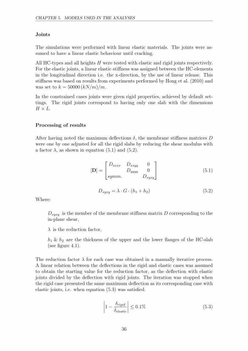
Joints

The simulations were performed with linear elastic materials. The joints were as-sumed to have a linear elastic behaviour until cracking.

All HC-types and all heights H were tested with elastic and rigid joints respectively.For the elastic joints, a linear elastic stiffness was assigned between the HC-elementsin the longitudinal direction i.e. the x-direction, by the use of linear release. Thisstiffness was based on results from experiments performed by Hong et al. (2010) andwas set to k = 50000 (kN/m)/m.

In the constrained cases joints were given rigid properties, achieved by default set-tings. The rigid joints correspond to having only one slab with the dimensionsH × L.

Processing of results

After having noted the maximum deflections δ, the membrane stiffness matrices Dwere one by one adjusted for all the rigid slabs by reducing the shear modulus witha factor λ, as shown in equation (5.1) and (5.2).

[D] =

Dxxxx Dxxyy 0Dyyyy 0

symm. Dxyxy

(5.1)

Dxyxy = λ ·G · (h1 + h2) (5.2)

Where:

Dxyxy is the member of the membrane stiffness matrix D corresponding to thein-plane shear,

λ is the reduction factor,

h1 & h2 are the thickness of the upper and the lower flanges of the HC-slab(see figure 4.1).

The reduction factor λ for each case was obtained in a manually iterative process.A linear relation between the deflections in the rigid and elastic cases was assumedto obtain the starting value for the reduction factor, as the deflection with elasticjoints divided by the deflection with rigid joints. The iteration was stopped whenthe rigid case presented the same maximum deflection as its corresponding case withelastic joints, i.e. when equation (5.3) was satisfied.

∣∣∣∣1− δrigidδelastic

∣∣∣∣ ≤ 0.1% (5.3)

36

5.1. FLOOR JOINTS

5.1.2 Verification with hand calculation

The floor slabs were considered as deep beams since L/H < 3. Ordinary beamtheory is thus not applicable. The displacement of the floor slabs was approximatedby estimating the contributions from shear and bending separately.

Displacement due to shear

The displacement at mid-span due to shear in the concrete was approximated byintegration of the shear angle over half of the span length. Approximate sheardisplacement, for small angles γ:

δ ≈ γ · b (5.4)

Where:

b is the width, which is half the span length in this case.

The shear angle is expressed as:γ =

τ

G(5.5)

Where:

τ is the shear stress.

The shear force V (x) was assumed to vary linearly over the span. Regarding thethickness, the contribution from the web in resisting the shear force was neglectedand the thickness was taken as the thickness of the flanges only, which gives theexpression for τ as follows:

τ =V (x)

H · (h1 + h2)(5.6)

Where:

V (x) is the shear force,

H is the height of the beam,

h1 + h2 is the thickness of the flanges.

Substituting equation (5.5) and (5.6) into (5.4) and integrating over half the spanof the beam gives the deflection due to shear at mid-span as:

37


δshear =

∫ L/2

0

V (x)

G ·H · (h1 + h2)dx (5.7)

q = 5kN/m

L

H

V

x

δshear

Figure 5.6 Shear displacement.

Displacement due to bending

Ordinary beam theory was used to estimate the deflection due to bending. Deflectionat mid-span:

δbending =5qL4

384EI(5.8)

Where:

q is the load,

L is the span length of the beam,

I is the moment of inertia.

38

5.1. FLOOR JOINTS

δbending

q = 5kN/m

L

H

Figure 5.7 Bending displacement.

Displacement in the joints

An elastic stiffness based on experimental values was assumed for the joints as in thefloor analyses with RobotTM in section 5.1.1. In the experiment performed by Honget. al. (2010) cracking load and displacement are presented for joints in hollow coreslabs subjected to in-plane loading. The stiffness used for the joint was taken as:

k =Pcr/2

δcr· H

Htest

(5.9)

Where:

Pcr is the cracking load,

δcr is the deformation at the cracking load,

Htest is the height of the beam in the experiment.

The displacement at mid-span was calculated as the summation of the displacementof each joint:

δjoint =5∑

i=1

∆δ(xi) =5∑

i=1

V (xi)

k(5.10)

39


δjoint

q = 5kN/m

L

H

V

x1 x2 x3 x4 x5

Figure 5.8 Shear displacement in the joints.

Total displacement at mid-span

For the rigid joints the total displacement was calculated as the sum of the shear inthe material and the deflection due to bending. For the elastic joint the displacementin the joints was added as well.

Displacement at mid-span with rigid joints:

δtot = δshear + δbending (5.11)

Displacement at mid-span with elastic joints:

δtot = δshear + δbending + δjoint (5.12)

5.2 Shear key joints

Because of the varying dimensions of precast wall elements, joints between shearwalls are not placed with standard distances as the joints between HC-elements. It

40

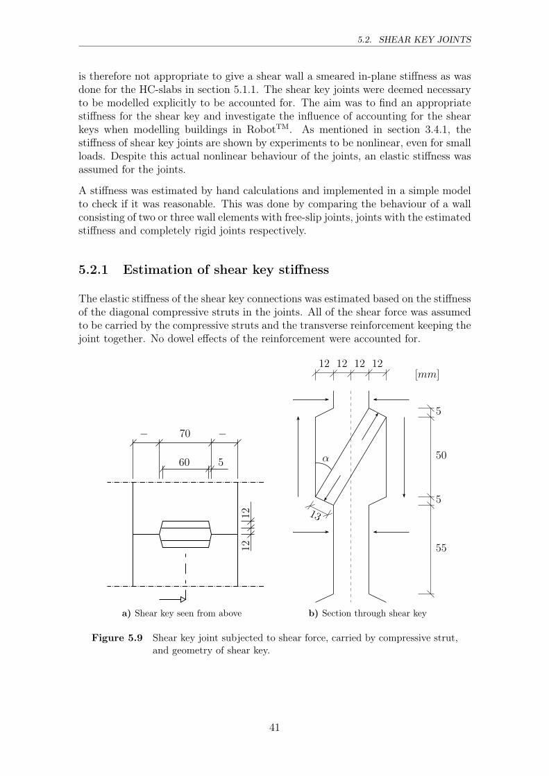
5.2. SHEAR KEY JOINTS

is therefore not appropriate to give a shear wall a smeared in-plane stiffness as wasdone for the HC-slabs in section 5.1.1. The shear key joints were deemed necessaryto be modelled explicitly to be accounted for. The aim was to find an appropriatestiffness for the shear key and investigate the influence of accounting for the shearkeys when modelling buildings in RobotTM. As mentioned in section 3.4.1, thestiffness of shear key joints are shown by experiments to be nonlinear, even for smallloads. Despite this actual nonlinear behaviour of the joints, an elastic stiffness wasassumed for the joints.

A stiffness was estimated by hand calculations and implemented in a simple modelto check if it was reasonable. This was done by comparing the behaviour of a wallconsisting of two or three wall elements with free-slip joints, joints with the estimatedstiffness and completely rigid joints respectively.

5.2.1 Estimation of shear key stiffness

The elastic stiffness of the shear key connections was estimated based on the stiffnessof the diagonal compressive struts in the joints. All of the shear force was assumedto be carried by the compressive struts and the transverse reinforcement keeping thejoint together. No dowel effects of the reinforcement were accounted for.

60 5

70− −

1212

a) Shear key seen from above

12 12 12 12

α

5

50

5

55

[mm]

13

b) Section through shear key

Figure 5.9 Shear key joint subjected to shear force, carried by compressive strut,and geometry of shear key.

41


The stiffness of one compressive strut derived from Hook’s law:

ki =EA

L(5.13)

Where:

A is the cross-sectional area of the compressive strut,

L is the length the compressive strut.

The total stiffness of the joint in the longitudinal direction:

k =n∑

i=1

ki · cos(α) (5.14)

Where:

n is the number of shear keys in the joint,

α is the inclination of the compressive strut.

The number of shear keys per joint was determined based on the fact that approx-imately 2m of the wall height is made with castellated shear keys, according to amanufacturer. The geometry of the shear key on which the calculations were basedis presented in figure 5.9 above.

The estimated stiffness of the shear key was verified by comparison to experimentalresults from the literature described in section 3.4.1 Stiffness of shear key joints.

5.2.2 Wall model

A test to evaluate the estimated stiffness and investigate the influence of jointsbetween shear walls was performed. The model consisted of a 5m (B) wide and30m (H) high cantilever wall with one or two vertical joints (see figure 5.10 below).

Simulations were performed for four different joint conditions. (1) The joint wasdefined by assigning a linear release, to allow free slip between the elements. (2)The joint was assigned an elastic linear release with a stiffness corresponding to alower limit of experimental stiffness summarised by Olesen (1975). (3) The estimatedvertical stiffness calculated in section 5.2.1 was assigned to the joint by an elasticlinear release. (4) The joint was defined as rigid by default settings.

The lower limit of experimental stiffness is presented in the literature as τ/δ. How-ever the stiffness input in RobotTM is on the form (kN/m)/m, why the stiffnesspresented in the literature was processed as follows:

k =τ

δ· A · 1

Hwall

= 2 · 2 · 0.07 · 1

3= 0.09 (GN/m)/m (5.15)

Where:

42

5.2. SHEAR KEY JOINTS

A is the shear area, taken as the cross sectional area of the joint in the longi-tudinal direction as 2m× 70mm,

Hwall is the height of the wall, which is 3m.

The impact of using different stiffness of the joints was measured by studying thevertical reaction forces in the foundation and the horizontal displacement in theupper right node and comparing the results from the different cases. The resultswere compared to see if the estimated stiffness gave a performance in between thefree-slip and rigid cases as intended.

P

P

P

P

P

P

P

P

P

P

H

B

a) One joint

P

P

P

P

P

P

P

P

P

P

H

B

b) Two joints

Figure 5.10 Test set-up for the shear key wall test.

43


Table 5.3 Shear key wall test configuration.

Loads

The test model was subjected to point loads P on each floorlevel with a magnitude of 35 kN which correspond to windload on a ∼ 20m wide façade divided on three stabilisingwalls just as in the building model described in section 5.3and appendix B.

Geometry Each wall element was 3m high which gave the total heightH = 30m.

Calculation

The mesh was rendered with Coons’ method as 4-nodequadrilaterals with a size of 0.2m, see figure 5.11. Thecalculation was of the 2:nd order with P-delta analysis andthe method used in RobotTM was chosen to multi-threadedsolver.

Concrete The concrete was of class C50/60 with properties describedin section 5.1.1, table 5.2.

Figure 5.11 Wall model with mesh. The mesh is shown for the wall model withone vertical joint.

44

5.3. BUILDING MODEL

5.3 Building model

To test the influence of the reduction factor obtained from the test described in sec-tion 5.1.1 and the estimated stiffness of the wall shear keys described in section 5.2.2on a larger structure, a test-model of a 10-storey high building with one stabilisingcore and one shear wall was set up. The purpose of this model was to investigatehow the joints affect the load distribution. The vertical reaction forces in the groundsupports were studied when the properties of the floors and walls were changed. Thegeometry of the test model is presented in appendix B.

Figure 5.12 Building model presented in 3D.

45


Wall

Core

Column

y xz

Figure 5.13 Load resisting members.

The ground supports was categorised by the three different load receiving parts.Wall, Columns (12 pc) and Core (see figure 5.13). After having run a test, thevertical reaction forces in the ground support nodes were summarised by equation(5.16) below for each load resisting member.∑∣∣Fz,i

∣∣ (5.16)

46

5.3. BUILDING MODEL

5.3.1 General model settings

Table 5.4 Building model configuration.

LoadsThe load was applied as a linear load on each floor witha magnitude of 5 kN/m along the edge parallel with they-axis, see figure 5.12, and as self-weight of the structure.

Supports

Beam-column: The beams were simply supported by thecolumns and continuous over non-end columns,

Slab-beam: The slabs were simply supported by the beams,

Slab-wall: The slabs were simply supported by the walls.

Ground supports Pinned supports were assigned to the columns, the coreand the wall.

Beams

217

20020

496

8 20040

E = 210GPa

G = 210GPa

fy = 355MPa

[mm]

Columns300

20010

E = 210GPa

G = 80.8GPa

fy = 355MPa

[mm]

Calculation

The mesh was rendered with Coons’ method as 4-nodequadrilaterals with a size of 0.5m, see figure 5.14. Thecalculation was of the 2:nd order with P-delta analysis andthe method used in RobotTM was chosen to multi-threadedsolver.

47


Figure 5.14 Building model with mesh.

5.3.2 Floor joint settings

Three different floors were used in the model, these are described in table 5.5 below.The first one was a solid slab that corresponds to the floor used in Model A ofHotel Hagaplan, the second floor was defined as the predefined hollow slab panel inRobotTM and the third floor represented a floor with joints, by reducing the shearstiffness. The impact of the different floors was measured by studying the verticalreaction forces on the stabilising elements and comparing them. Joints between wallelements were rigid during this test.

48

5.3. BUILDING MODEL

Table 5.5 Floors used in building model.

Floor 1 (F1)

Consisted of solid concrete with a thickness of 200 mm.The concrete class was of C50/60 with properties describedin section 5.1.1, table 5.2 except for the self-weight whichwas reduced to 16.5 kN/m2 to correspond to a HC-floorwith the same thickness.

Floor 2 (F2) Defined in RobotTM in the same way as in section 5.1.1with dimensions of the slab HD/F 120/20 in table 5.2.

Floor 3 (F3)

Defined in RobotTM as a user-defined panel with a stiff-ness matrix similar to F2 but with an in-plane shear stiff-ness reduced with a reduction factor λ of 0.12 which wasobtained from the results of the test of floor joints, for a200mm thick slab.

5.3.3 Wall joint settings

Joints were introduced in the stabilising members, as shown in figure 5.15 below,where four different degrees of stiffness, described in table 5.6, were applied. Thereaction forces in the stabilising elements were studied in the same way as for theslabs in section 5.3.2 and the slabs were set to the configuration F2 (HC-floor) for allwall tests. The results of these tests are presented in section 6.3.2. A combinationwhere both the wall joints and the floor joints were accounted for was performedas well. In these tests the floors were modelled as floor type F3, see table 5.5,with modified in-plane shear stiffness and the walls were modelled with the fourdifferent stiffnesses presented in table 5.6. The results for this combined analysisare presented in section 6.3.3.

49


Joint

y xz

Figure 5.15 Load resisting members with joints.

Table 5.6 Configuration of wall joints in the building model.

Rigid jointBy the use of default settings in RobotTM, a rigid con-nection between the walls was defined for the joint, whichcorresponds to one continuous wall.

Lower limitelastic joint

An elastic stiffness obtained by estimation described in theprevious section 5.2.1 was assigned for the interface be-tween the walls, by defining a linear release with elasticproperties.

Estimatedelastic joint

An elastic stiffness obtained by estimation described in theprevious section 5.2.1 was assigned for the interface be-tween the walls, by defining a linear release with elasticproperties.

Free slipThe interface between the walls was defined by a linear re-lease to allow free slip in the longitudinal direction betweenthe walls.

50

Chapter 6

Results from the analyses

The results of the simulations with the FE-models and hand calculations are pre-sented and explained in this chapter. The following results are illustrated: thein-plane deformations and the reduction factor of the floor model, the deformationsand reaction forces of the wall model, and the deflections of the top floor and thereaction forces of the walls in the building model.

6.1 Behaviour of floor model

6.1.1 Deflections, FE-simulations

The slabs with thickness 270 and 320mm performed almost the same deflection inboth the elastic and the rigid cases, why it can be difficult to separate them in figure6.1 below. It may seem illogical that two plates with different thickness have almostthe same performance, but by studying equation (4.3) and figure 4.1, it is shownthat the membrane stiffness D of a hollow core slab in RobotTM depends highly onthe flange thickness (h1 + h2) of its cross section. (h1 + h2) had a value of 76 and72mm for the 270 and 320mm thick slabs respectively. The membrane stiffnessD also depends on the equivalent height heqv of the slabs which is greater for thethickness of 320mm as seen in table 5.1. These two parameters may explain thesimilar results for the two thicknesses.

The three elastic curves in 6.1 have higher slopes than the rigid ones and are thereforemore dependent of the relation of L/H. The difference between the elastic and therigid curves represents the deformation of the joints. For a higher slab (small L/H)the total stiffness of the joint was greater than for a lower slab, as the stiffness wasdefined per meter joint in the longitudinal direction. This explains why the elasticcases are more dependent of the length to height ratio.

51

CHAPTER 6. RESULTS FROM THE ANALYSES

0 0.5 1 1.5 2 2.50

0.05

0.1

0.15

0.2

0.25

0.3

0.35

0.4

L/H

Deflection

[mm]

Elastic 200 mmElastic 270 mmElastic 320 mmRigid 200 mmRigid 270 mmRigid 320 mm

Figure 6.1 Deflection for different length/height relations of the floor.

6.1.2 Deflections, Hand calculations

The hand calculation resulted in lower deflections in every point compared to theresults in RobotTM. The pattern that the slabs with a thickness of 270 and 320mmfollow each other was also present in the hand calculations but there was no steadydistance between them and the curve for 200mm. Instead, they began at almost thesame deflection for L/H ∼ 1 to then develop differently for increasing L/H. A reasonfor this is probably the estimation of the bending deflection in the hand calculations(equation 5.8 in section 5.1.2). The phenomena of a deep beam are more prominentwhen decreasing L/H and the equation for bending deflection becomes more appli-cable when increasing L/H. The hand calculations were very approximative andwere used only to give an indication of that the FE-results were reasonable.

52

6.1. BEHAVIOUR OF FLOOR MODEL

The shear deformations of the joints estimated by hand calculation agreed very wellwith the FE-results.

0 0.5 1 1.5 2 2.50

0.05

0.1

0.15

0.2

0.25

0.3

0.35

0.4

L/H

Deflection

[mm]

Elastic 200 mmElastic 270 mmElastic 320 mmRigid 200 mmRigid 270 mmRigid 320 mm

Figure 6.2 Hand calculated deflection for different length/height relations of thefloor.

Why RobotTM gives 45% higher values can partly be a result of problems due tosingularities close to the supports which cause large concentrations of stresses. Thisis an effect not acting in the hand calculations. Initially, the configuration of thetest rig was not taking this phenomenon in consideration and no mesh refinementsand extra beams were inserted by the supports. After having found the source oferror and looking deeper into the deformed shape close to the supports in RobotTM,it was discovered visually that the elements close to the supports stood for a majorpart of the total deflection. The improvements in the model around the supports ledto a better looking deformed shape but the singularities were still present. Figure6.3 shows the deformed shape of the floor model obtained from RobotTMbefore andafter the improvements of the model.

53


With improvements

Without improvements

Figure 6.3 Mesh improvements in the floor model.

6.1.3 Reduction factor

The reduction factor λ for the shear member of the membrane stiffness matrix Dis presented in figure 6.4. The pattern from figure 6.1 also appear in the plot forthe reduction factor regarding that the thickness of 270 and 320 mm have generallythe same values. By studying the plot, it can be assumed that the reduction factordepends more on the thickness of the flanges (h1 + h2) than on the relation of L/Hat least for large L/H.

The curve for 200 mm changes shape when it passes L/H = 1, while the othercurves do not. There might be several reasons for this, but one has to remem-ber that this cross-section is not designed to act in this span length according toBetongelementföreningen (1998).

54

6.2. BEHAVIOUR OF WALL MODEL

0 0.5 1 1.5 2 2.5

0.08

0.1

0.12

0.14

0.16

L/H

λ[-]

200 mm265 mm320 mm

Figure 6.4 Reduction factor λ.

6.2 Behaviour of wall model

The stiffness of the vertical shear key joint was estimated to 5.57GN/m, see Ap-pendix C for calculations. This provided a stiffness for the linear release in RobotTM

of 1.86 (GN/m)/m as the estimated stiffness divided by the height of the wall. Thestiffness from the Olesen (1975) summary vary between (0.27− 4.01)GN/m, whichis less than the estimated stiffness. However, these reflect the actual nonlinear be-haviour of the joint and are defined by a secant of the load-displacement curvecorresponding to two thirds of the ultimate load, for lower loads the stiffness wouldbe higher. Furthermore, the stiffness depend on the geometry of the shear keys,which differs both among the joints in the summary of experiments and to the jointthat formed the basis for the estimation.

A calculation according to Bljuger (1976) gives an elastic stiffness of one joint of(3.23− 5.11)GN/m. The interval is provided by a lack of precision of the definitionof Fk, which therefore was applied as two alternative areas, see Appendix C.

The estimated stiffness was, based on the comparison to the literature regarded asa reliable approximation. However, since much lower stiffness of joints have beenobserved, the lower limit value was applied in the model as well, to observe howlarge impact the choice of stiffness have on the wall behaviour. As can be seen infigure 6.5, the deflection was similar for the walls with joints with the estimatedelastic stiffness, the joints with the lower limit experimental stiffness and the rigidjoints.

The discovered pattern between the deflection of the models with one and two jointsis an increased deflection for each linear stiffness tested, which is shown in figure 6.5(a) and 6.5 (b) below. When free slip is applied in the joints (k = 0), the deflectiondeveloped dramatically compared to the other rigidities but this is an unrealistic

55


condition and will not be further discussed.

The relation between the deflections of the completely rigid and the free-slip casesagreed with beam theory. Based on deflections of a cantilever beam the wall withone free-slip joint should give four times the deflection of the wall with a rigid joint.For the case with two joints the free-slip case should give nine times the deflectionof the rigid case.

The deflections for the wall with a thickness of 300mm was (in average) -32% smallerthan the deflections for the 200mm thick wall. As the wall was increased by a thirdin thickness, the deflection was reduced with a third, it was thereby concluded thatthe thickness of the wall had a linear impact on the deflection. Therefore, the resultsare only presented for the wall of 200mm thickness.

The calculated stiffness of 1.857GN/m2 gave a deflection that lies between the wallwith rigid joints and the lowest value of k found in the literature. This gave anindication that the model, developed in section 5.2.1 about the shear key joint,provided reliable results and was worth proceeding with in the building model.

56


200 3000

50

100

150

200

71.09

47.41

22.08 15.8618.11 12.1617.85 11.9

Wall thickness [mm]

Displacment[mm]

Free, k = 0 (GN/m)/m

Elastic, k = 0.09 (GN/m)/m


Rigid, k = −

a) One vertical joint

200 3000

50

100

150

200

162.13

108.16

25.0918.7618.33 12.3517.88 11.92

Wall thickness [mm]

Displacment[mm]




Rigid, k = −

b) Two vertical joints

Figure 6.5 Deflections in the upper right corner of the wall model described insection 5.2.2.

The deformed shapes of the wall with one joint assigned different stiffnesses areshown in figure 6.6. These deflections correspond to the values in figure 6.5 (a).Figure 6.6 shows that the wall with a free-slip joint acts as a series of two beams,while the walls with a stiffness assigned to the joint interact across the joint.

57


a) Free, k = 0 b) Elastic, k = 0.09 (GN/m)/m

c) Elastic, k = 1.857 (GN/m)/m d) Rigid, k = −

Figure 6.6 Deflection of the wall model with one joint.

The vertical reaction forces in the walls are plotted in figure 6.7. The magnitudesof the forces in the estimated elastic and the rigid cases differs very little, whilethe free-slip and lower limit stiffness gave considerably greater forces. The resultof deformations in the elastic joint is shown by the dodge on the curve, where

58


the generally linear behaviour is departed from. The shapes of the curves were asexpected according to Olesen (1975). As deformations in the wall elements wereconsidered the curve was expected to have a steeper inclination close to the ends,such that the curve was not linear, but rather of third order.

0 1 2 3 4 5−600

−400

−200

0

200

400

600

[m]

[kN

]

a) k = 0 (GN/m)/m

0 1 2 3 4 5−600

−400

−200

0

200

400

600

[m]

[kN

]

b) k = 0.09 (GN/m)/m

0 1 2 3 4 5

−300

−200

−100

0

100

200

300

[m]

[kN

]

c) k = 1.857 (GN/m)/m

0 1 2 3 4 5

−300

−200

−100

0

100

200

300

[m]

[kN

]

d) Rigid k = −

Figure 6.7 Vertical reaction forces from the shear wall test with one joint. Thedashed vertical line indicates the position of the joint in the wall.

59


6.3 Behaviour of building model

6.3.1 Influence of floor joints

Figure 6.8 and 6.9 below shows the distribution of the vertical reaction forces be-tween the stabilising elements and the columns, for a load case of wind plus self-weight and wind only, respectively. The three different floors that were modelledare represented by the three column types in the figures. During these analyses thewall joints were rigid. The distribution of the forces in the case when the self-weightand the wind load was taken into account indicated that the columns were takingthe majority of the total vertical forces. The difference between modelling the floorsas solid with reduced self-weight compared to modelling them as HC-slabs gave adifference of ≤ ± 3.23 % in each member for the load case with both wind and self-weight. The difference in reactions between the HC-slab and the modified HC-slabwas obtained as < ± 0.02 %. The perimeter beams around the floors may have con-tributed to that the effects of accounting for the joints were so small. The beamshad a stiffness in the horizontal direction that resists in-plane deflection of the floor.The linearly pinned connection between the beams and the floors which satisfiescompatible displacements and no slip between the elements may also influence theresults.

Core Wall Columns0.00

20.00

40.00

60.00

80.00

100.00

24.28

7.39

68.33

26.41

8.50

65.09

26.40

8.50

65.10

[%]

F1 - Solid floorF2 - HC-floorF3 - HC-floor with modified stiffness

Figure 6.8 Force distribution in load resisting members due to a load combinationof self-weight and wind load parallel to the y-axis. F1, F2 and F3 aredescribed in section 5.3.2.

60

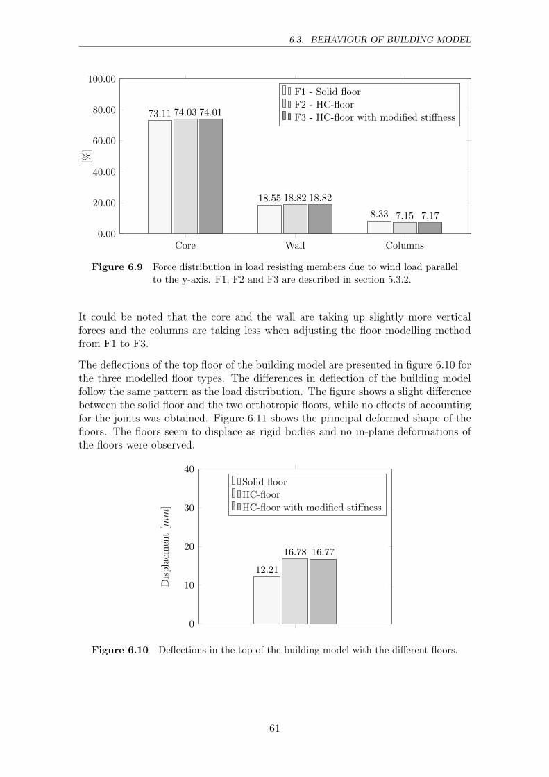
6.3. BEHAVIOUR OF BUILDING MODEL

Core Wall Columns0.00

20.00

40.00

60.00

80.00

100.00

73.11

18.55

8.33

74.03

18.82

7.15

74.01

18.82

7.17

[%]

F1 - Solid floorF2 - HC-floorF3 - HC-floor with modified stiffness

Figure 6.9 Force distribution in load resisting members due to wind load parallelto the y-axis. F1, F2 and F3 are described in section 5.3.2.

It could be noted that the core and the wall are taking up slightly more verticalforces and the columns are taking less when adjusting the floor modelling methodfrom F1 to F3.

The deflections of the top floor of the building model are presented in figure 6.10 forthe three modelled floor types. The differences in deflection of the building modelfollow the same pattern as the load distribution. The figure shows a slight differencebetween the solid floor and the two orthotropic floors, while no effects of accountingfor the joints was obtained. Figure 6.11 shows the principal deformed shape of thefloors. The floors seem to displace as rigid bodies and no in-plane deformations ofthe floors were observed.

0

10

20

30

40

12.21

16.78 16.77

Displacment[mm]

Solid floorHC-floorHC-floor with modified stiffness

Figure 6.10 Deflections in the top of the building model with the different floors.

61


a) Solid b) HC-slab c) HC-slab, modified stiffness

Figure 6.11 Deformed shape of the 7th floor in the building model.

6.3.2 Influence of wall joints

Figure 6.12 and 6.13 show the distribution of vertical reactions to the load resistingmembers when the building model was subjected to a combination of wind loadand self-weight, and only wind load respectively. During these tests the floors weremodelled as floor type F2, i.e. hollow core slabs with no consideration of the joints.The four tested degrees of linear stiffness for the wall joint resulted in very smalldifferences, even between rigid and free-slip joints.

Core Wall Columns0

20

40

60

80

100

26.77

8.84

64.39

26.74

8.83

64.42

26.66

8.83

64.5

26.43

8.58

64.99

[%]




Rigid, k = −

Figure 6.12 Load distribution in supporting members due to a load combinationof self-weight and wind load parallel to the y-axis.

62


Core Wall Columns0

20

40

60

80

100

74.03

18.77

7.2

74.02

18.78

7.2

73.99

18.79

7.22

74.06

18.73

7.22

[%]




Rigid, k = −

Figure 6.13 Load distribution in supporting members due to wind load parallelto the y-axis.

The vertical reaction forces in the stabilising wall are presented in figure 6.14 below.The difference between the reactions are small just as for the force distribution infigure 6.12 and 6.13, and the stiffness of the joints seems to not affect the verticalreaction forces. The same applies to the deflection of the building model, presentedin figure 6.15. The corresponding deformed shapes of the wall are shown in figure6.16. The shapes are basically the same for all stiffnesses assigned to the joint, andno slip or deformation in the vertical joint was observed.

The results of the building model with rigid wall joints should be the same as theresults obtained in section 6.3.1 for floor type F2, when the three floor types weretested. However, a difference of 2% was obtained for the deflection in these twocases. One possible explanation for this difference in result could be that the newmesh that was generated for the building model when the wall joints were introduceddiffered from the mesh before.

63


0 1 2 3 4 5−100

−75

−50

−25

0

25

50

75

100

[m]

[kN

]

a) k =∼ 0 (GN/m)/m

0 1 2 3 4 5−100

−75

−50

−25

0

25

50

75

100

[m]

[kN

]b) k = 0.09 (GN/m)/m

0 1 2 3 4 5−100

−75

−50

−25

0

25

50

75

100

[m]

[kN

]

c) k = 1.857 (GN/m)/m

0 1 2 3 4 5−100

−75

−50

−25

0

25

50

75

100

[m]

[kN

]

d) Rigid k = −

Figure 6.14 Vertical reaction forces on the shear wall in the building model. Thedashed vertical line indicates the position of the joint in the wall.

64


0

10

20

30

40

16.41 16.41 16.4 16.39Displacment[mm]




Rigid, k = −

Figure 6.15 Deflections of the top floor of the building model.

a) Free-slip, k = 0 b) k = 0.09 (GN/m)/m c) k = 1.86 (GN/m)/m d) Rigid, k = −

Figure 6.16 Deflection of the wall in the building model with joints of differentstiffness.

A possible explanation for the low influence from the vertical joints is the connectionbetween the wall and the slab on every floor. In RobotTM, this connection wasdefined as simply supported which could counteract the walls to have an unevenvertical displacements. Looking at figure 6.17 below, it can be observed that themodel with free-slip joint in the walls was generating shear forces in the slab whilethe rigid joints did not. In the results in RobotTM only out-of-plane shear forceswere available and not out-of-plane shear stresses. This indicated that the floor slabshas been calculated based on Kirchhoff theory, which results in that no out-of-planeshear deformations in the slabs have been accounted for. The slab would thereforenot allow any vertical shear deformations in the wall joints.

65


Column

a) k = − (rigid)

V ertical joints

Column

b) k =∼ 0 (free-slip)

Figure 6.17 Shear force concentration for a floor plan.

66


6.3.3 Combination of floor joints and wall joints

The following results were obtained from the analyses when the floor joints wereaccounted for by a reduced in-plane shear stiffness and four different degrees ofstiffness were assigned to the wall joints.

The distribution of vertical reaction forces between the supporting members is pre-sented in figure 6.18 and 6.19, for the load cases with wind load and self-weight,and only wind load respectively. Figure 6.20 shows the deflection of the top floorof the building model. Just as in the previous section all cases resulted in similaroutcomes and no considerable effects were obtained from accounting for the floorand wall joints in combination.

Core Wall Columns0

20

40

60

80

100

26.68

8.77

64.56

26.65

8.76

64.59

26.57

8.76

64.67

26.56

8.76

64.68

[%]

Free joint, k =∼ 0

Elastic joint, k = 0.09 (GN/m)/m


Rigid joint, k = −

Figure 6.18 Load distribution in supporting members due to a load combinationof self-weight and wind load parallel to the y-axis.

Core Wall Columns0

20

40

60

80

100

73.99

18.85

7.17

73.98

18.85

7.17

73.94

18.88

7.18

73.93

18.89

7.19

[%]

Free joint, k =∼ 0



Rigid joint, k = −

Figure 6.19 Load distribution in supporting members due to wind load parallelto the y-axis.

67


0

10

20

30

40

18.81 18.81 18.8 18.79Displacment[mm]




Rigid, k = −

Figure 6.20 Deflections in the top of the building model.

68

Chapter 7

Discussion

7.1 RobotTMmodels

Some warnings were obtained during the analysis of the floor model and the buildingmodel. The models suffered from instabilities of type 3 which means that some valuesof the stiffness matrix are very disproportional. This is the result of very largedifferences in stiffness from one element to another. According to recommendationsfrom Autodeskr support, this type of error can be neglected.

When using any type of FEM program singularities can be a problem. The floormodel suffered from singularities at the supports in its initial set-up but after mod-ifications the load was spread out over more elements which reduced the problem.The fact that singularities are difficult to get rid of without affecting the model canbe taken as a possible reason why the RobotTM model performed greater deflectionsin figure 6.1 than the hand calculations in figure 6.2.

This thesis aimed at finding both the actual stiffness of joints and a way to implementthem in RobotTM for design. This means that the reality is searched regarding thestiffness, while the models should reflect common engineering practice. This is whythe mesh is not chosen based on a convergence study, but rather on what is practicalin an early stage design. Furthermore, the wind was simplified to an equivalent staticaction and as a result all simulations were performed with static analysis, since thisis common practice for buildings.

A limitation in RobotTM is that contact surfaces cannot be modelled. More infor-mation about the behaviour of the joint could have been obtained in an other FEMsoftware, in which the joint could be modelled with its geometrical and materialproperties in combination with the adjacent elements.

The results of the models have been verified by comparison to theory, which indicatedthat the results of the models were as expected. The differences were explained bythe different assumptions and simplifications in the calculation methods.

69

CHAPTER 7. DISCUSSION

7.2 Floor joints

The stiffness of the floor joints applied in the models are based on only one source.There may be reasons to believe that the stiffness could vary between differentexperiments and that the stiffness used in the model is not the actual stiffness.However, the model simulations clearly show that the diaphragm action of the plateis not influenced by the change of stiffness of the floor, and this is likely to have beenthe outcome even for a slightly different stiffness, as the in-plane shear stiffness wasreduced with close to 90%.

The stiffness of the floor joint used in the models was obtained from an experimentof a HC-slab with a thickness of 200mm. This stiffness was used for all the HC-slabsin the models, and thereby no consideration was taken regarding that joints in slabswith different thickness have different stiffness.

When the equivalent stiffness of the floor was developed, only the in-plane shearstiffness was changed but it is possible that the behaviour of the floor is affectedin more ways by the joint. Other parameters that were evaluated to be reducedwere the Young’s modulus and the height, but these would affect the out-of-planebehaviour as well and were therefore considered inappropriate, since this behaviourwas not studied. By reducing the in-plane stiffness in the membrane matrix, thestiffness is reduced in both the longitudinal and the transversal direction of theslab. The transverse direction was however not intentionally reduced, but this wasconsidered to be an assumption on the safe side.

The nonlinear behaviour and influence of cracks in the joints were neglected in theanalysis. The stiffness used in the models corresponds to the uncracked state, butin reality the joints might be cracked. However, the load was chosen to produce astress level below the shear strength of the joints.

7.2.1 Floor joints in the building model

There is a possibility that the influence of the joints is more considerable for buildingsof a different shape or with other configurations of stabilising shear walls and cores.For slender buildings with shear walls with a homogeneous stiffness, the assumptionof a completely rigid floor diaphragm have been proven to be applicable and forthese cases the stiffness of the floor should not be of great importance. However,for buildings with shear walls which have large openings or in other ways containsdrastic changes in stiffness, the stiffness of the floor may be significant for the loaddistribution.

The effects of the perimeter beams surrounding the floor in the building model wasnot investigated. The ability of these beams to resist in-plane deformations may beof interest for the stiffness of the diaphragm.

70

7.3. WALL JOINTS

7.3 Wall joints

Just like in the case with the floor model a great uncertainty surrounds the chosenstiffness of the joint. The stiffness estimated based on experimental results lieswithin an extremely large interval. What the differences in the results depend on isdifficult to determine since all set-up data for the experiments were not obtained.The geometry and material of the joint are likely to affect the stiffness, as was shownin the method for estimating the stiffness with compression struts. According tothe literature, shear key joints have been produced in various designs, and this isprobably reflected in the experiments summarised by Olesen (1975). Depending onthe material used for the joints in the experiments and whether or not it had non-shrink properties that prevents shrinkage cracks, different results should be expectedregarding the stiffness.

For these reasons the estimated stiffness was considered appropriate to take further.However, because of the uncertainty of the chosen stiffness, the lower limit valueobtained from the literature was applied in the wall model as well. This providedan interval which most certainly contains the actual stiffness. A comparison of theresults from these cases therefore reflect the effects of the real stiffness.

The estimation of the stiffness of the joint was based on the formation and stiffnessof the compressive strut, and depended on the dimensions and geometry assumedfor the compressive strut. The cross-sectional area of the compressive strut waschosen as the smallest possible to be on the safe side. Still the estimated stiffnesswas greater than the experimental.

The experimental stiffness is expressed in the literature as τ/δ, while the estimatedstiffness and the input to RobotTM is on the form V/δ. Thus the experimentalstiffness needed to be multiplied with the shear area. One source of error may bethe choice of shear area. The shear area was chosen as the cross-sectional area ofthe joint, however other options could have been to use the cross-sectional area ofthe whole wall or only the area of the keys.

The stress levels in the joint have not been analysed nor has the strength propertiesor failure modes of the joint. The joint was assumed to act in a linear elastic phase,which results in a linear relation between stress and strain even when the strengthis exceeded.

7.3.1 Shear key joints in the building model

A worst case scenario was modelled in the building model regarding the positionsof the joints. The joints were placed on top of each other on the same vertical line,while the joints in reality usually are placed at different positions on each floor toincrease the shear capacity. The results from the building model regarding the shearkeys therefore represent the maximum effects of the joints. However, the results forthe vertical reaction forces in the supporting nodes for the stabilising walls were

71

CHAPTER 7. DISCUSSION

almost the same for every joint stiffness.

Regarding the reaction forces in the wall model and the building model, the slabsare thought to be the source of the different shapes. The explanation that the slabscontributes with a locking effect for the shear deformations in the joints was con-cluded by studying figure 6.17 and by looking at an exaggerative deformed shape ofthe wall. The fact that the rigid and free-slip wall joint differ so little in result inthe building model while they perform considerable differences in the wall model,gave reason to question if the behaviour had been correctly captured. The theoryon which the calculation of the slabs were based, controls how out-of-plane sheardeformations are handled. The slabs in the models were most likely based on Kirch-hoff theory. As the out-of-plane shear deformations of the plate are thought to beimportance for the behaviour of the wall with joints the Mindlin theory would havebeen preferred, but a choice of theory was not known to be available. The behaviourof the building probably depends on how the connection between the walls and theslab behaves which has not been studied in this thesis. The behaviour of this connec-tion depends very much on its design, which in turn varies according to the globaldesign of the structure. Better knowledge about such connections and especiallyits behaviour in a material nonlinear analysis would make the analysis of the walljoints in the building model more reliable. With nonlinear material behaviour, thestress redistributions and deformations caused by cracks and local failures could beincluded in the model.

7.4 Hotel Hagaplan

The problem of the contribution of the columns to the stabilising actions was notsolved by taking the joints into account in the model. The problem is thought tobe a result of the behaviour of the floors in the models. The attempt to make apinned connection between the floors and the shear walls or cores, and between thefloors and the columns, in order to leave the columns out of the stabilising action,is possibly counteracted by the parts of the floor that encircles the core. This isbelieved to be the reason why what seems to be a pinned frame stabilised by a wallin 2D, actually can create tensile forces in the pinned columns in 3D.

According to Fröderberg (2011) the overestimation of frame action can be avoidedby reducing the bending stiffness to close to zero for the relevant members. Othersolutions to this problem could be to use other methods for modelling the buildingwhere the columns are excluded, and the load on the shear walls and cores areapplied manually.

7.5 Conclusions

The general conclusion of all the tests is that the load distribution is not affectedwhen the joints are accounted for in a RobotTM model for the type of building that

72

7.6. FURTHER RESEARCH

was treated in this thesis, since neither the reduction factor of the floor, nor theapplied stiffness in the wall joints resulted in significant changes in the results. It ishowever not concluded that the joints do not influence the behaviour of FE-modelsof buildings with other shapes or configuration of stabilising walls.

When modelling buildings in RobotTM with the purpose of accounting for the walljoints, it is not enough to only model the stiffness of the wall joints if the floor slabsare rigidly connected to the walls in the longitudinal direction of the connection. Inthis case the connection between the wall and the slab must be adjusted to allowthe shear deformations of the joint.

It has also been shown that what does affect the quality of the model are reasonableboundary conditions and keeping the model simple enough to enable convergence ofsecond order analysis.

7.6 Further research

The aim of this thesis was to go deeper into FE-modelling of precast concrete struc-tures and investigate how assumptions of the joints affect the total stability of abuilding by studying the load distribution. The investigations of the joints betweenHC-slabs and between shear walls are just two aspects and to receive a reliablepicture about the total stability, more assumptions have to be investigated. Onesuggestion for further research is to investigate the connection between the shearwalls and floors, to determine to what extent this connection counteract the de-formations between the wall elements. Further investigations could be performedregarding how the nonlinear behaviour of the materials, and the formation of cracks,influence the load distribution.

To reach a solution to the problem with columns contributing to the stabilisingaction, different methods for calculations and modelling could be investigated andcompared. This could include evaluating assumptions and simplifications in orderto receive a reliable load distribution of the lateral forces.

73

Bibliography

Ansell, A., Hallgren, M., Holmgren, J., Lagerblad, B., Westerberg, B., 2014. Con-crete Structures. Report 143, Stockholm: KTH Civil and Arcitechtural Engineer-ing.

Autodesk Inc., 2016a. User’s Guide. [online] AutodeskRobot Structural Analysis Professional Help. Available at:http://help.autodesk.com/view/RSAPRO/2016/ENU/?guid=GUID-4A734308-B2F3-4147-A310-BD47C48E9ED1 [Accessed 8 Apr. 2016].

Autodesk Inc., 2016b. What’s new 2016. [online] AutodeskRobot Structural Analysis Professional Help. Available at:https://knowledge.autodesk.com/support/robot-structural-analysis-products/learn-explore/caas/CloudHelp/cloudhelp/2016/ENU/RSAPRO-WhatsNew/files/GUID-105E3920-BB99-4AA7-A4B5-CE98B24929A1-htm.html[Accessed 25 Apr. 2016].

Bachmann, H., Steinle, A., 2011. Precast Concrete Structures. Berlin: Wilhelm Ernstand Sohn, Verlag für Architektur und technische Wissenschaften.

BCA, 2001. Structural Precast Concrete Handbook. 2nd ed. Technology DevelopmentDivision of the Building and Construction Authority.

Betongelementföreningen, 1998. Bygga med prefab: En handbok i teknik, estetik,kvalitet, ekonomi och miljö. Bromma: Betongelementföreningen.

Bhatt, P., 1973. Influence of vertical joints on the behaviour of precast shear walls.Building Science, 8(3), pp.221–224.

Bljuger, F., 1976. Determination of deformability characteristics of vertical shearjoints in precast buildings. Building and Environment, 11(4), pp.277–282.

Buettner, D. R., Becker, R. J., 1998. PCI Manual for the Design of Hollow CoreSlabs. 2nd ed. Chicago: Precast/Prestressed Concrete Institute.

Cook, R. D., Malkus, D. S., Plesha, M. E., Witt, R. J., 2001. Concepts and Appli-cations of Finite Element Analysis. 4th ed. Hoboken, NJ: John Wiley and sons,Inc.

Elliott, K. S., Jolly, C. K., 2013. Multi-Storey Precast Concrete Framed Structures.2th ed. Oxford: Blackwell Publishing Ltd.

75

BIBLIOGRAPHY

Fröderberg, M., 2011. Stabilitetsberäkningar med FEM - Metodbeskrivning . Malmö:Tyréns AB.

Ghosh, S. K., Fanella, D. A., 2003. Seismic and Wind Design of Concrete Buildings.USA: International Code Council, Inc.

Heyden, S., Dahlblom, O., Olsson, A., sandberg, G., 2008. Introduktion till Struk-turmekaniken. Lund: Studentlitteratur AB.

Hong, G.-H., Baek, J.-S., Park, H.-G., 2010. Shear performance evaluation of thejoint between hollow core slabs. Journal of the Korea institute for structural main-tenance and inspection, 14(4), pp.94–101.

Isaksson, T., Mårtensson, A., Thelandersson, S., 2010. Byggkonstruktion. 2nd ed.Lund: Studentlitteratur AB.

Lorentsen, M., Petersson, T., Sundquist, H., 2000. Stabilisering av byggnader. 6thed. Stockholm: Institutionen för Byggkonstruktion. Kungliga Tekniska Högskolan.

Memon, B. A., Su, X. Z., 2004. Arc-length technique for nonlinear finite elementanalysis. Journal of Zhejiang University. Science, 5(5), pp.618–628.

Mendis, P., Ngo, T., Haritos, N., Hira, A., 2007. Wind loading on tall buildings.Electronic Journal of Structural Engineering, Special Issue: Loading on Struc-tures, pp.41–54.

Olesen, S., 1975. Effects of vertical keyed shear joints on the design of reinforcedconcrete shear walls. ACI Special Publication, 48(5), pp.85–110.

Pacoste, C., 2015. Lecture 5 - Plate bending and shell elements Lecture slides incourse: AF2024 "Finite Element Methods in Analysis and Design 7.5 credits" -Spring 2015. Stockholm: Kungnliga Tekniska Högskolan.

Park, R., Paulay, T., 1975. Reinforced Concrete Structures. Hoboken, NJ: JohnWiley and Sons, Inc.

PCI, 2007. Designing with Precast and Prestressed Concrete. Chicago: Pre-cast/Prestressed Concrete Insitute.

Pekau, O., 1981. Influence of vertical joints on the earthquake response of precastpanel walls. Building and Environment, 16(2), pp.153–162.

Prestrud, O., Cholewicki, A., 1969. Model tests on shear walls composed of prefab-ricated concrete elements. Symposium CIB "Bearing Walls", Warsaw.

Roper, S. C., Iding, R. H., 1984. Appropriateness of the rigid floor assumption forbuildings with irregular features. In: Proc. 8th WCEE, San Francisco, Vol.4. pp.751–758.

SS-EN 1168:2005+A3:2011, 2011. Precast concrete products – Hollow core slabs.Stockholm: SIS Förlag AB.

76

BIBLIOGRAPHY

SS-EN 1990, 2010. Eurocode – Basis of structural design. Stockholm: SIS FörlagAB.

SS-EN 1991-1-4:2005, 2008. Eurocode 1: Actions on structures – Part 1-4: Generalactions – Wind actions. Stockholm: SIS Förlag AB.

Strängbetong, 2014. Håldäck. [online] Strängbetong. Available at: http://www.strangbetong.se/koncept-komponenter/komponenter/bjalklag/haldack/[Accessed 02 Jun. 2016].

Westerberg, B., 1999. Stomstabilisering, Kurskompendium. Stockholm: Tyréns Byg-gkonsult AB.

77

Appendix A - Comparison betweenthe two original models of HotelHagaplan

A.1 Model A

Model A (figure A.1) has pinned connections between the columns and the beams,these connections are defined in RobotTM with releases. The internal beams aremodelled continuously over the columns. The horizontal connections between thewalls at each floor level are modelled as pinned by the use of linear releases. Nolinear releases are defined for the floor, meaning that it is fixed to the beams. Theground supports in the model are pinned for both columns and walls.

Shell elements are used to represent the floor slab and the walls. The beams andcolumns are modelled with beam elements. The floor is modelled as a continuoussolid concrete slab floor with adjusted self-weight to account for the voids in thehollow core slab. The concrete quality C35/45 is used for the floor. The walls aremodelled with C35/45 quality concrete with stiffness properties reduced with respectto cracking.

79

BIBLIOGRAPHY

Figure A.1 Model A.

A.2 Model B

In model B (figure A.2) the walls and floor parts are modelled separately with asmall distance in between. Principally the four walls forming a core are separatedin this way and the floor is divided by the beams. The connections between theseelements are modelled with small concrete beam elements. The small beam elementsthat connect the floor slabs to the beams and the walls have a fixed connection

80

A.2. MODEL B

inside the floor and where they connect to the beams or walls they are released forrotation in all directions and for displacement in the vertical direction, except inthree connections per floor element where the displacement in the vertical directionis fixed to prevent the floor from falling down. The elements that connect the wallsto each other have no assigned releases. The beams are pinned to the columns andthe walls.

Figure A.2 Model B.

As in model A the walls and floors are represented by shell elements and the beamsand columns are represented by beam elements. The floor is modelled with thehollow core slabs defined in RobotTM. Concrete quality C50/60 are used for the

81

BIBLIOGRAPHY

walls and no reduction for cracks have been made in the material properties.

A.3 Evaluation of differences

The first step in finding a simple way to model precast concrete structures was tofind out what was causing the results from the two models to differ. When firstlooking at the models it could be observed that model A showed large tensile andcompression forces in the columns when the building was subjected to horizontalloading. This result indicated that the columns took part in the stabilising action.For precast concrete structures the columns are assumed to only transfer verticalloads because of their pinned connections and limited ability to transfer momentsBCA (2001). The stabilising system should in this case be formed by the walls only.Model B showed very small forces in the columns when subjected to horizontalloading only. This model had achieved a more correct load distribution between thecolumns and the walls with respect to horizontal loads. The lateral loads appliedto the models were checked and found to be principally of the same magnitude forthe two models. The two models different ways to distribute the horizontal loads inthe linear analysis was assumed to essentially be a result of how the connections aremodelled.

A.3.1 Connections

A series of tests was set up to investigate the influence of the connections on the loaddistribution of the lateral load between the walls and the columns. The geometry forthe test models was chosen as a part of the Hotel Hagaplan building. The floor planis presented in appendix B, figure B.1, a wall on the left edge of the model and a coreconsisting of three walls formed the stabilising members. The floor was modelledsupported by beams. Columns were placed along the perimeter and internally tosupport the beams. A horizontal load was applied along the sides of the floor.Initially one storey was analysed, this storey was then copied to form a ten-storeystructure, to account for the behaviour of a slender structure.

The connection conditions for the test series is presented in table A.1 below. Inthe first test model every connection between the members was modelled as fixedand the floor slab was continuous over the beams i.e. the floor was modelled inone piece and not divided by the beams. In the following test models, more andmore releases were assigned to the connections. The last test model has connectionsmodelled with small beam elements, similar to those of model B, which allows notonly for rotation around the edge of the member but for rotation in the othertwo orthogonal directions as well. These connections were created with a spacingbetween the members and were used in the wall to wall connection, the wall to slabconnection and the slab to beam connection.

82

A.3. EVALUATION OF DIFFERENCES

Table A.1 Connection properties in the test models.

Test

Supp

orts

Colum

nto

beam

Beam

tobe

am

Wallt

owall

Floor

tobe

am

Floor

divide

dby

beam

s

Con

nections

mad

eof

beam

elem

ents

0 Fixed Fixed Fixed Fixed Fixed No No1 Pinned Fixed Fixed Fixed Fixed No No2 Pinned Pinned Fixed Fixed Fixed No No3 Pinned Pinned Pinned Pinned Pinned No No4 Pinned Pinned Pinned Pinned Pinned Yes No5 Pinned Pinned Pinned Pinned Pinned Yes Yes

The influence of the connections on the load distribution between the walls andcolumns was investigated by looking at the reaction forces on walls and columnsrespectively. The vertical reactions on all the columns are presented in table A.2as the percentage of the total reactions. The reactions on the walls are presentedcorrespondingly.

Table A.2 Vertical reactions in the supports of the test models.

TestReactions on

the columns [%]Reactions onthe walls [%]

0 17.0 83.01 16.9 83.12 13.7 86.33 11.5 88.54 7.5 92.55 7.8 92.2

The results principally showed that the more releases assigned to the model the lessdid the columns participate in the stabilising action.

A.3.2 Second-order effects

Another factor influencing the diverse results was thought to be how the secondorder effects in the two models are handled. No second order analysis is performedon model B, while these effects are considered in model A.

Model B was run with second order analysis (P-delta analysis) without achievingconvergence. In order to achieve convergence in the analysis the model was simpli-fied. A part of the model with just two storeys was analysed and an attempt to

83

BIBLIOGRAPHY

correct the warning messages were made. Different solvers and calculation methodswere tested. This simplified model was sent in to the RobotTM support team fromwhere some changes such as deleted releases was presented which made the anal-ysis converge. Applying these changes on the full model did not help in achievingconvergence. Deleting all releases did give a converged solution. The reason for thefailure to reach convergence could be that the model is too complex with respect toits connections and that there are too many releases in the model.

A.3.3 Stiffness of the walls and columns

A third aspect that differs between the two models that is thought to have effect onthe differences in results are the stiffness of the walls and columns.

A.4 Conclusion

Based on the investigation of these models it is clear that building a FE-model ofa precast concrete structure is not a trivial task. The initial starting point thatmodel B had captured the behaviour of the structure in a desirable way has beenabandoned. Shortcomings in both models have been found. This investigationwas not thorough enough to determine exactly what caused the models to givedifferent results but it provided guidance on how to direct the further work. Oneof the common issues in the differences between the models was found to be theflexibility and stiffness of the structures. Connections and joints are special featuresof precast concrete structures which affects the stiffness of the structure as a whole.Furthermore, the ability to include second-order effects are affected by how theconnections are modelled.

84

Appendix B - Drawings of thebuilding model

y

x

7090

7023

6627

6650

2220

7380

4490

5960 3250 6200

Figure B.1 Floor plan of the building model [mm].

85

BIBLIOGRAPHY

y

x

3000

3000

3000

3000

3000

3000

3000

3000

3000

3000

Figure B.2 Section of the building model [mm].

86

Appendix C - Calculations

C.1 Deflection of deep beam

q = 5 kN/mL = 12mH = {5, 7, 9, 11, 13}m

h = {104.3, 142.19, 152.52 }mm(h1 + h2) = {50, 76, 72 }mm

G = 15416.7MPaE = 37000MPa

Deflection at mid-span due to shear:

δshear =

∫ L/2

0

V (x)

G ·H · (h1 + h2)dx =

q(L/2)2

2 ·G ·H · (h1 + h2)

Deflection at mid-span due to bending:

δbending =5qL4

384EI=

5qL4

384E · h ·H3

12

The stiffness of the joints:

k =Pcr/2

δcr· H

Htest

=35.2/2 · 103

0.32 · 10−3· H

1.1= 50000H kN/m

The deflection at mid-span due to deformations of the joints:

δjoint =

5∑i=1

∆δ(xi) =

5∑i=1

V (xi)

k=

5∑i=1

q(L/2− x)

k

Displacement at mid-span with rigid joints:

δtot,rigid = δshear + δbending

87

BIBLIOGRAPHY

Displacement at mid-span with elastic joints:

δtot,elastic = δshear + δbending + δjoint

Table C.1 Calculated deflection for all floor heights and cross-sections.

Plate Height Shear Bending Joint TOT Rigid TOT elasticH δshear δbending δjoint δtot,rigid δtot,elastic

HD/F 120/20 5 0.039 0.233 0.240 0.272 0.512HD/F 120/27 5 0.025 0.153 0.240 0.179 0.419HD/F 120/32 5 0.027 0.162 0.240 0.189 0.429HD/F 120/20 7 0.028 0.085 0.171 0.113 0.284HD/F 120/27 7 0.018 0.056 0.171 0.074 0.245HD/F 120/32 7 0.019 0.059 0.171 0.078 0.250HD/F 120/20 9 0.023 0.050 0.133 0.074 0.207HD/F 120/27 9 0.015 0.033 0.133 0.048 0.182HD/F 120/32 9 0.016 0.035 0.133 0.051 0.184HD/F 120/20 11 0.019 0.028 0.109 0.047 0.156HD/F 120/27 11 0.013 0.018 0.109 0.031 0.140HD/F 120/32 11 0.013 0.019 0.109 0.032 0.141HD/F 120/27 13 0.011 0.014 0.092 0.025 0.118HD/F 120/32 13 0.012 0.015 0.092 0.027 0.119

88

C.2. STIFFNESS OF SHEAR KEY JOINT

C.2 Stiffness of shear key joint

12 12 12 12

α

5

50

5

55

[mm]

13

a) Shear-key

d

L

hα

b) Strut

Figure C.1 Geometry of shear key and compressive strut.

Geometry and material properties:

α = arctan( 3 · 12

50 + 5

)= 0.579 rad

L =√

(3 · 12)2 + (50 + 5)2 = 65.734mm

h =√

122 + 52 = 13mm

d = 60mm

A = d · h = 60 · 13 = 780mm

E = 33000MPa

n =length of joint

legnth of shear key=

2000

50 + 5 + 5 + 55= 17

The stiffness in the axial direction of one compressive strut derived from Hook’s law:

ki =EA

L=

33000 · 780

65.734= 0.392 · 106 kN/m

The total stiffness of the joint in the vertical direction:

89

BIBLIOGRAPHY

k =

n∑i=1

ki · cos(α) = 17 · 0.392 · 106 · cos(0.579) = 5.57 · 106 kN/m

The stiffness for a linear release in RobotTM was defined per meter joint. The totalstiffness of the joint in the vertical direction per meter joint for a 3m high wall:

k =5.57 · 106

3= 1.86 · 106 (kN/m)/m

C.2.1 Processing of stiffness found in the literature

Stiffness of Olesen (1975) literature summary:τ

δ= 2 · 106 − 30 · 106 kN/m3 k =

τ · Aδ

A = Shear area = 60 · (13 + 50 + 13 + 55)

Stiffness of one key:ki = 0.015 · 106 − 0.24 · 106 kN/m

Stiffness of one joint (2m):k = 0.27 · 106 − 4.01 · 106 kN/m

Stiffness according to Bljuger (1976):Ekg = 3.3 · 105 kg/cm2 Fk = 5 · 6 + 2 · 1.3 · 6 = 45.6 cm2

Alternatively:Fk = 5 · 6 = 30 cm2

The area Fk is not unambiguously defined or presented in the literature.

Stiffness of one key

k =Ekg · Fk

50=

3.3 · 105 · 45.6

50= 3.01 · 105 kg/cm = 0.30 · 106 kN/m2

Alternatively:

k =Ekg · Fk

50=

3.3 · 105 · 30

50= 1.98 · 105 kg/cm = 0.20 · 106 kN/m2

Stiffness of one joint:k = 5.11 kN/m

Alternatively:k = 3.23 kN/m

90

Documents

Modelling Lateral Stability of Prefabricated Concrete ...kth.diva-portal.org/smash/get/diva2:940461/FULLTEXT01.pdfModelling Lateral Stability of Prefabricated Concrete Structures Caroline