Embed Size (px)
Citation preview

Modelling Land Use in Rural New Zealand
Alex Olssen & Suzi Kerr Motu Economic and Public Policy Research
[email protected] [email protected]
Paper presented at the 2011 NZARES Conference
Tahuna Conference Centre – Nelson, New Zealand. August 25-26, 2011
Copyright by author(s). Readers may make copies of this document for non-commercial purposes only, provided that this copyright notice appears on all such copies

Draft Modelling Land Use in Rural New
Zealand Alex Olssen and Suzi Kerr
NZARES Conference 2011 Motu Economic and Public Policy Research
August 2011

i
Author contact details Alex Olssen Motu Economic and Public Policy Research [email protected]
Suzi Kerr Motu Economic and Public Policy Research [email protected]
Acknowledgements We would like to thank Max Aufhammer from the University of California Berkeley for suggestions at a presentation of an earlier version of this paper. We are also indebted to Arthur Grimes for many useful discussions. Of course, all remaining errors are our own.
Motu Economic and Public Policy Research PO Box 24390 Wellington New Zealand
Email [email protected] Telephone +64 4 9394250 Website www.motu.org.nz
© 2011 Motu Economic and Public Policy Research Trust and the authors. Short extracts, not exceeding two paragraphs, may be quoted provided clear attribution is given. This paper has been circulated for purposes of information and discussion. It has not necessarily undergone formal peer review or editorial treatment. ISSN 1176-2667 (Print), ISSN 1177-9047 (Online).

ii
Abstract New Zealand rural land is dominated by four major uses – dairy farming, sheep and beef farming, plantation forestry, and unproductive scrub. Using national time series data we look at how each of these land uses has responded to changing economic returns, as measured by relevant commodity prices, over the period from 1974 to 2008. We do this by developing a dynamic econometric model which relates rural land use to economic factors. We follow the literature on the estimation of dynamic singular equation systems. We adopt this framework to look at land use choices. Our coefficients provide preliminary estimates of the responsiveness of different types of rural land to changing economic returns. They are used to compare different carbon price scenarios.
JEL codes Q15, Q24
Keywords Land use change, New Zealand, National, time series

1
1. Introduction
Rural land use is a major determinant of economic and environmental outcomes in New
Zealand. In 2010 around 5 per cent of New Zealand’s GDP was due to agricultural, or forestry
production1
New Zealand rural land is dominated by four major uses – dairy farming, sheep and beef
farming, plantation forestry, and unproductive scrub. Using national time series data we look at
how each of these land uses has responded to changing economic returns, as measured by
relevant commodity prices, over the period from 1974 to 2008. We do this by developing a
dynamic econometric model which relates rural land use to economic factors. We follow the
literature on the estimation of dynamic singular equation systems (Anderson and Blundell (1982),
(1983)). Singular equation systems have often been estimated to model consumer expenditure
patterns – expenditure and savings always add up to income. We adopt this framework to look at
land use choices – the sum of rural land in each use always adds up the total amount of rural
land.
, both of which use rural land as a key input. On the environmental side, agricultural
production is a large source of Greenhouse Gas (GHG) emissions while forestry is an emissions
sink. Despite this there is little research investigating the economic determinants of rural land use
in New Zealand.
Our coefficients provide preliminary estimates of the responsiveness of different types of
rural land to changing economic returns. In other work, we use these estimates to look at
different carbon price scenarios. The small quantity of data is a potential problem for our
research. However our results seem sensible and have an intuitive interpretation. Long-run own-
price elasticities are typically positive while cross-price elasticities are typically negative. In the
short-run there seems to be a split between productive and non-productive land uses, with all
types of productive rural land use increasing with increases in any commodity prices, and non-
productive rural land decreasing with increases in any commodity prices.
The rest of this paper is structured as follows. In section 2 we develop a theoretical
model of land use choice at a parcel level, and show what this implies for aggregate land use.
Section 3 describes our data and looks at summary statistics and graphs. Cointegration tests are
reported in section 4. In section 5 we present our econometric methodology. Section 6 contains
estimation results, including our tests of dynamic simplifications. Section 7 presents a baseline
land use scenario until 2050. In section 8 we conclude.
1 This number was calculated using data from Statistics New Zealand that can be accessed at www.stats.govt.nz/infoshare/

2
2. Theoretical framework
2.1. Individual land use choices
We solve a dynamic land allocation problem. Our model follows the models of Stavins
and Jaffe (1990) and Parks (1995) closely. Consider a land manager who has a fixed quantity of
land denoted by 𝐴 making a plan for her land at time 𝑡 = 0. She takes the proportion of her
total land in each of 𝑘 uses at the initial period, denoted by 𝑎𝑖0 where 𝑖 = 1, . . . , 𝑘, as given (this
would be the case if she had only just become the land manager, or she were reconsidering her
land use choices in which case her old choices are then given). She chooses non-land inputs
(which we have supressed for clarity – the results are qualitatively unchanged) and the amount of
land to transfer between each use, 𝑧𝑖𝑗𝑡 ∀ 𝒊 ≠ 𝒋, to solve the following problem:
𝐦𝐚𝐱
{𝒛𝒊𝒋𝒕}𝐢≠𝐣� ∞
𝟎��
𝒌
𝒊=𝟏
𝝅𝒊(𝒂𝒊𝒕) −� 𝒌
𝒊=𝟏
� 𝒌
𝒋≠𝒊
𝑪𝒊𝒋(𝒛𝒊𝒋𝒕)�𝒆𝜹𝒕𝐝𝒕, ( 1 )
subject to
𝑨 = �
𝒌
𝒊=𝟏
𝒂𝒊𝒕, ∀ 𝒕 ( 2 )
𝒂𝒊𝒕 ≥ 𝟎, ∀ 𝒊, 𝒕 ( 3 )
�̇�𝒊𝒕 = �
𝒌
𝒋≠𝒊
𝒛𝒊𝒋𝒕 −� 𝒌
𝒋≠𝒊
𝒛𝒋𝒊𝒕, ∀ 𝒊, 𝒕 ( 4 )
𝒛𝒊𝒋𝒕 ≥ 𝟎, ∀ 𝒊, 𝒋, 𝒕 ( 5 )
𝑎𝑖𝑜 a given constant, ∀𝑖.
Expression ( 1 ) gives the net present value for any set of decisions about land
conversions. 𝝅𝒊(𝒂𝒊𝒕) and 𝑪𝒊𝒋(𝒛𝒊𝒋𝒕) are both increasing functions of their arguments. We assume that
land managers are able to borrow to fund conversions and such debt is repayed over the lifetime
of the investments - this is included in the function 𝑪𝒊𝒋(𝒛𝒊𝒋𝒕). Constraint ( 2 ) says that in every
time period 𝒕 total land 𝑨, which is assumed to be constant over time, is equal to the sum of all
land used for production 𝒂𝒊𝒕 - this means we are assuming that conversion, 𝒛𝒊𝒋𝒕, is instantaneous.
Constraint ( 3 ) ensures the amount of land in each use is nonnegative. Constraint ( 4 ) is the law
of motion which determines how the land use shares, 𝒂𝒊𝒕, evolve over time. The change in the
amount of land in use 𝒊 is equal to the sum of all land transfered into use 𝒊 minus the sum of all
land transferred out of use 𝒊. Constraint ( 5 ) is a nonnegativity constraint which ensures the 𝒛𝒊𝒋𝒕

3
have the interpretation as the amount of land moving from use 𝒋 to use 𝒊 - this clearly cannot be
negative even though net land transfer between use 𝒊 and use 𝒋 can be negative.
The current value Hamiltonian for this model is given by
𝑯 = ��
𝒌
𝒊=𝟏
𝝅𝒊(𝒂𝒊𝒕)−� 𝒌
𝒊=𝟏
� 𝒌
𝒋≠𝒊
𝑪𝒊𝒋(𝒛𝒊𝒋𝒕)�+ � 𝒌
𝒊=𝟏
𝝀𝒊𝒕 �� 𝒌
𝒋≠𝒊
𝒛𝒊𝒋𝒕 −� 𝒌
𝒊≠𝒋
𝒛𝒋𝒊𝒕�. ( 6 )
The first order conditions are
𝛛𝑯𝛛𝒛𝒊𝒋𝒕
= −𝑪𝒊𝒋′ (𝒛𝒊𝒋𝒕) + 𝝀𝒊𝒕 − 𝝀𝒋𝒕 = 𝟎. ( 7 )
𝛛𝑯𝛛𝒂𝒋𝒕
= 𝝅𝒋′(𝒂𝒋𝒕) = −��̇�𝒋𝒕 − 𝜹𝝀𝒋𝒕�. ( 8 )
To confirm the −𝝀𝒋𝒕 in ( 7 ) term simlpy expand constraint ( 4 ) before differentiating.
Condition ( 7 ) determines optimal conversion and by setting it to zero we are implicitly
assuming an interior solution. While corner solutions are likely to be important for individual
land managers we use data on national time series in which corner solutions are irrelevant.
Multiplying ( 7 ) by 𝛿 and substituting 𝛿𝜆𝑖𝑡 from ( 8 ) gives
𝜹(𝝀𝒊𝒕 − 𝑪𝒊𝒋′ (𝒛𝒊𝒋𝒕)) = 𝝅𝒋′(𝒂𝒋𝒕) + �̇�𝒋𝒕. ( 9 )
We see that at an optimum the marginal benefit (net of annualised conversion costs) of
an extra hectare in the new use 𝑖, given by 𝛿(𝜆𝑖𝑡 − 𝐶𝑖𝑗′ (𝑧𝑖𝑗𝑡)), must equal the marginal cost of an
extra hectare in the original use 𝑗, given by the direct marginal profit of an extra hectare in the
old use 𝜋𝑗′(𝑎𝑗𝑡), plus future gains to returns in the old use �̇�𝑗𝑡 . This result is very similar to Parks
(1995) where �̇�𝑗𝑡 is interpreted as capital gains. All land with returns that exceed a threshold will
be put into the new use and this happens at every threshhold.
Importantly this model predicts instantaneous land use change. In practice land use
change can be slow. Stavins and Jaffe (1990) suggest forest age distribution, liquidity constraints,
uncertainty about the permanence of price movements, and decision-making inertia as possible
reasons for slow land use adjustment. When we specify our econometric model later we will
include dynamics to allow for slow land use change.
2.2. Aggregation
The model above implies that all parcels of a given quality with the same prospects for
capital gains should have the same land use. In this work we use national time series data. Land
use differs across New Zealand. Stavins and Jaffe (1990) suggest two reasons for heterogeneous

4
land use in aggregate land areas; firstly land use may be adjusting towards a steady state; secondly
there is unobservable heterogeneity in land and farmers.
An important question is how we can make predictions about land use at the national
level from our parcel level model. This is a classic case of the aggregation problem faced by
econometricians. Stavins and Jaffe (1990) first answered this question for county level data. They
assumed a distribution of land quality and showed how changes in flood protection projects
affected land quality and hence land use. In our work we are interested in the effect of economic
returns on land use choices. We don’t model the distribution of land quality as changing, but
only have in mind that as economic returns change, the amount of land that should be allocated
to different uses will change. Suppose the price of the good associated with land use 𝑖 increased.
Because profit includes revenue this will increase the right-hand side of ( 9 ). Then because
𝐶𝑖𝑗(𝑧𝑖𝑗𝑡) is increasing the optimal level of 𝑧𝑖𝑗𝑡 would fall – i.e., if the price associated with use 𝑖
increased then the amount of land converted from use 𝑖 to use 𝑗 would fall. Similar dynamics
apply to �̇�𝑖𝑡 as well as things that might affect the function 𝐶𝑖𝑗(𝑧𝑖𝑗𝑡).
3. Data
3.1. Data sources
We need two main types of data: data on the area of land in each rural use, and data on
economic variables which we expect to be associated with land use. Our data comes from a
variety of sources.
3.1.1. Land area data
Rural land use data for New Zealand has been collected in various ways in recent history.
Statistics New Zealand (SNZ) conducted the Agricultural Production Census for the years 1974
to 1987, 1990, 1994, 2002, and 2007. They also conducted sample surveys for the years 1988,
1989, 1991 to 1993, 1995, 1996, 1999, 2003 to 2006, and 20082
2 The survey that was conducted in 1999 had a different population base and so we did not use it.
. Unfortunately SNZ did not
collect land area data at even the national level for 1997, 1998, 2000, or 2001. However the Meat
and Wool Economic Service used their own surveys to construct national level data designed to
be consistent with SNZ’s Agricultural Production Statistics data for 2000 and 2001. They
estimated national land use areas in 1997 and 1998 using linear interpolation. Thus, using these
sources as well as land area data published by SNZ in 1972 and 1973 provides us with a time
series of observations on rural land areas.

5
This time series does not distinguish between farm land used for dairy production as
opposed to sheep and beef meat production. Because dairy production and sheep and beef meat
production are very different in terms of their economic and environmental effects we want to
model these separately. For the years 1980 to 1996, 2000, 2001, and 2002, Meat and Wool
separated pasture land in to dairy land, sheep and beef land, and other pastoral land, at the
national level by using data on average farm size and total farm numbers. We split pasture in the
remaining periods between dairy and sheep and beef land by extrapolating based on animal
numbers.
Data on the land area in plantation forestry is mostly available from the SNZ – however
the period from 1997 to 2001 is again an exception. The National Exotic Forestry Description
(NEFD) has data on the amount of new land converted into plantation forestry as well as the
amount of land deforested over this period. Thus we combine plantation forestry area data on
levels from SNZ in 1996 and 2002, with data on changes from NEFD between 1997 and 2001
to estimate the amount of land in plantation forestry between 1997 and 2001.
We estimate the area of scrub land as the residual of total rural land less the amount of
land used for grazing animals, for plantation forests, or for horticulture. The amount of land in
rural uses has changed over the passed few decades. Among other things, this is due to increases
in urban land and changes in conservation land. We expect changes in the total amount of rural
land to be primarily driven by factors other than economic returns in rural uses. We define a new
category, other land, which measures these exogenous changes in rural land relative to 1974.
other_land𝑡 = total_rural_land1974 − total_rural_land𝑡
Thus when other_land𝑡 > 0 we have total_rural_land𝑡 < total_rural_land1974. Thus
if other_land𝑡 is increasing then total_rural_land𝑡 is decreasing. We end up with a time series
on the area of New Zealand land in each of the four major rural uses – dairy farming, sheep and
beef farming, plantation forestry, and scrub, and a measure of the changes in total rural land.
3.1.2. Commodity prices
SNZ published data on the volume and value of agricultural exports in all years for
which we have land use data. This allows us to back out the export price in cents per kilogram
for each agricultural product of interest. Importantly, much agricultural production was
subsidised until 1990. We increase our prices over the period of subsidisation by weighting
factors, documented by Anderson (2007), which reflect the proportion of farm profits due to
government assistance. This gives us a time series of effective prices faced by farmers by land use

6
for the period 1972 to 2008. For dairy and forestry land the raw prices we use are the export
price in cents per kilogram of milk solids, and cents per cubic metre of wood. For sheep-beef we
use a composite price which is the weighted average of the price in cents per kilogram for sheep
meat, beef meat, and wool, where we weight by volume sold.
3.1.3. Other macroeconomic indicators
SNZ also collects data on Gross Domestic Product measured in various ways. The
Reserve Bank of New Zealand (RBNZ) has data on the interest rate of 5 year bonds as well as
exchange rates. These macroeconomic variables could be important for land use decisions and
hence we try several specifications including them in different combinations. However, because
we only have 35 time observations and we estimate both short and long run effects we quickly
lose degrees of freedom. In our preferred specification we only include nominal interest rates.
We present results for several specifications in our appendix.
3.2. Summary statistics
In this section we present summary statistics for our data. Land data is presented as
shares of total rural New Zealand land in 1974. Price data is presented as log(real_price𝑡),
where we used the RBNZ’s CPI with base year 2008. Our data is annual and spans the period
from 1974 to 2008 inclusive, giving us 35 yearly observations on 4 land uses of interest. Table 1
presents means and standard deviations for data used in our analysis.
Table 1: Summary statistics
Variable Mean Std. Dev. Min Max dairy share 0.09 0.02 0.07 0.12 sheep-beef share 0.70 0.06 0.57 0.76 forestry share 0.08 0.02 0.03 0.11 scrub share 0.13 0.03 0.09 0.18 other share 0.01 0.05 -0.04 0.12 log(dairy price) 6.29 0.20 5.85 6.77 log(sheep-beef price) 6.55 0.25 6.16 7.00 log(forestry price) 9.65 0.24 9.09 10.13 interest rate 9.33 3.67 5.41 18.47
Several things are worth noting. Firstly sheep beef land accounts for the majority of land
use throughout the series – at it’s peak sheep beef land accounted for 76 per cent of rural New
Zealand land (as a percentage of total rural land in 1974). The change in rural New Zealand land
relative to 1974 has fluctuated, as shown by the fact that the share of other land has been both
7
positive and negative over the period. The mean reported for price variables is the mean of the
logs rather than the log of the mean.
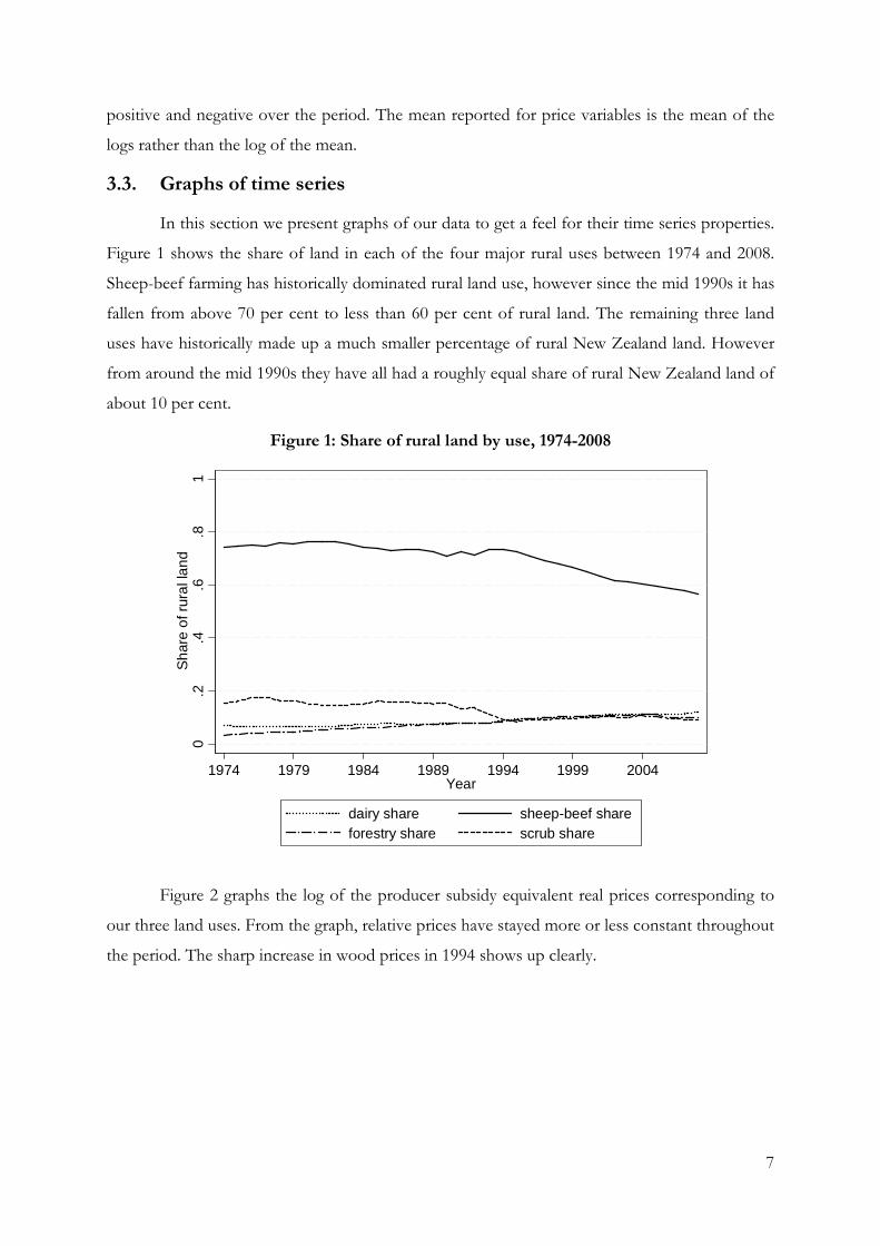
3.3. Graphs of time series
In this section we present graphs of our data to get a feel for their time series properties.
Figure 1 shows the share of land in each of the four major rural uses between 1974 and 2008.
Sheep-beef farming has historically dominated rural land use, however since the mid 1990s it has
fallen from above 70 per cent to less than 60 per cent of rural land. The remaining three land
uses have historically made up a much smaller percentage of rural New Zealand land. However
from around the mid 1990s they have all had a roughly equal share of rural New Zealand land of
about 10 per cent.
Figure 1: Share of rural land by use, 1974-2008
Figure 2 graphs the log of the producer subsidy equivalent real prices corresponding to
our three land uses. From the graph, relative prices have stayed more or less constant throughout
the period. The sharp increase in wood prices in 1994 shows up clearly.
0.2
.4.6
.81
Sha
re o
f rur
al la
nd
1974 1979 1984 1989 1994 1999 2004Year
dairy share sheep-beef shareforestry share scrub share

8
Figure 2: Real prices of agricultural products, 1974-2008
Figure 3 graphs the percentage change in the level of real producer subsidy equivalent
prices. The export price per cubic metre of wood product is far more volatile than either the
dairy export price or the sheep-beef export price.
Figure 3: Percentage change in real prices, 1975-2008
67
89
10R
eal p
rices
1974 1979 1984 1989 1994 1999 2004Year
log(dairy price) log(sheep-beef price)log(forestry price)
-100
0-5
000
500
1000
Per
cent
age
chan
ge in
real
pric
es
1975 1980 1985 1990 1995 2000 2005Year
percentage change in real dairy pricepercentage change in real sheep-beef pricepercentage change in real forestry price

9
3.4. Unit root tests
In this section we look at whether our land share, and price series are individually
stationary or not. Table 2 reports the test statistics for several Dickey-Fuller unit root tests as
well as the 5 per cent critical values.3
For each test the null hypothesis is that the univariate sequence contains a unit root. The
alternative hypothesis is that the series is stationary. We reject the null hypothesis if the test
statistic is smaller (more negative) that the critical value. Thus looking at the series as levels we
see that we cannot reject the null hypothesis of a unit root for any of the series except the
forestry share and the log(dairy price). From figure 1 it is clear that most of the land use time
series have reasonably strong trends over the period for which we have data. When we allow for
such trends we can only reject the null of a unit root in the series for log(dairy price).
The first two columns present test statistics for unit roots in
levels, where column (2) allows for a deterministic trend but column (1) does not. Columns (3)
and (4) present test statistics for first differences and column (4) allows for a trend while column
(3) does not.
Table 2: Unit root tests
Levels First differences
(1) (2) (3) (4)
dairy share 1.44 -2.61 -3.87 -4.33 sheep-beef share 2.14 -1.29 -4.56 -5.75 forestry share -3.03 1.97 -1.68 -2.37 scrub share -0.57 -1.98 -4.54 -4.49 other share 3.15 -2.01 -3.34 -5.73 log(dairy price) -3.16 -4.43 -7.88 -7.76 log(sheep-beef price) -1.63 -1.93 -5.64 -5.56 log(forestry price) -1.68 -3.09 -5.63 -5.60 interest rate -1.33 -2.41 -4.76 -4.94 critical value 5% -2.98 -3.56 -2.98 -3.56
While most of the series have unit roots in their levels, we can reject the null of unit
roots in favour of stationarity when we take first differences. Apart from the first difference in
the forestry share, all other differenced series have test statistics considerably more negative than
the critical values. Thus our series, with the possible exception of the forestry share, all appear to
be I(1).
3 More sophisticated tests for unit roots exist. For our data they all yield qualitatively similar results, with very few changes in rejection of the null hypothesis.

10
4. Cointegration tests
Given our time series appear to be I(1) it is natural to wonder whether some
combination of them are I(0). I.e., are there cointegrating factors amongst our time series which
we could think of us representing equilibrium tendencies? In particular we assume for each land
use there exists a long run equilibrium relationship of the form
𝑠𝑖𝑡 = 𝛼𝑖 +∑𝑗=13 𝛾𝑖𝑗 log�𝑝𝑗𝑡� + 𝛽𝑖1𝑖𝑡 + 𝛽𝑖2𝑠𝑜𝑡 + 𝜈𝑖𝑡 ( 10 )
where 𝑠𝑖𝑡 is the share of land in use 𝑖 at time 𝑡, 𝑝𝑗𝑡 is the price of the 𝑗-th commodity at
time 𝑡 − 14, 𝑖𝑡 is the nominal 5 year interest rate, 𝑠𝑜𝑡 is the share of other land, 𝜈𝑖𝑡 is ther error
term, and 𝛼𝑖, 𝛾𝑖𝑗, 𝛽𝑖1, and 𝛽𝑖2 are parameteres to be estimated.
We then test for cointegration by using panel unit root tests on the residuals from
regressions estimating the long run structure of our model, ignoring dynamic properties. We use
two panel unit root tests. One test is based on Choi (2001) and requires only 𝑇 → ∞
asymptotics. The null hypothesis is that the residuals of all equations have unit roots, and the
alternative is that at least one equation is stationary. This does not test cointegration directly but
uses appropriate asymptotics – if we cannot reject the null hypothesis this would be evidence
against cointegration. The second test is based on Hadri (2000). It requires 𝑇 → ∞ and then
𝑁 → ∞. Given we are only interested in four land uses this may not be appropriate. On the
other hand the hypotheses are appropriate. Under the null the residuals of all equations are
stationary, while under the alternative at least one has a unit root. These tests are both designed
as unit root tests (with differing null hypotheses) and we have made no adjustment to the p-
values to reflect that we are testing cointegration and multiple regressors in the first stage when
we calculate the residuals. However we hope these tests are indicative of whether it is reasonable
to think cointegration holds. Given three rural land shares and the amount of other land the
fourth land use is completely determined. Thus we implement these tests using residuals
obtained by estimating ( 10 ) by OLS for dairy, sheep-beef, and forestry land shares. We
implement the above two tests on the demeaned residuals using no lags, one lag or two lags.
Using the first method we reject the null hypothesis that all residual series have unit roots at the
5 or 10 per cent level for any lags. Using the second method we fail to reject the null that all
residual series are stationary at even the 10 per cent level using any of the above number of lags.5
4 Because land use decisions depend on expected future profitability under different uses lagged prices are often used to account for expectations formation – see footnote 5 of Miller and Plantinga (1999)
5 We used information from the Stata user manual – [xt] xtunitroot throughout this section.

11
5. Econometric methodology
We want to estimate the relationship between land use and commodity prices. I.e., how
does land use change at the national level as commodity prices change. It is useful to think in
terms of an allocation problem. Given current and expected economic returns over land uses
what is the best allocation of a particular parcel of land. Aggregating up to the national level we
want to know what share of rural land will be in each use given expected returns. This leads us
naturally to consider land use as a system of share equations. The share of land in each rural use
depends on the expected returns of land under each use. When the set of uses considered is
exhaustive and mutually exclusive such a system of equations is necessarily singular. With four
rural land uses (five if you include exogenous other land) we can always exactly infer the share of
land in the fourth use given the shares in the other three uses.
Dynamic considerations play an important role in our econometric specification. Land
use decisions now impact future options and profitability because of conversion costs for
example. This means that responses to economic conditions may have dynamic effects 6
Given the long run cointegrating relationship established in the previous section we
specify our general dynamic model as
.
Anderson and Blundell (1982) developed a methodology for incorporating general dynamics in
singular system estimation. Their method attractively nests several dynamic simplifications
allowing researchers to test whether a static model really is rejected by the data. Anderson and
Blundell (1983) is a good example of estimating such a general dynamic singular system. Ng
(1995) looks at cointegration within the Almost Ideal Demand System framework of the Deaton
and Muellbauer (1980), originally a static singular system of equations.
∆𝒔𝒕 = 𝑨∆𝒙�𝒕 − 𝑩(𝒔𝒕−𝟏 − 𝚷𝒙𝒕−𝟏) + 𝜺𝒕 ( 11 )
where, as analogues to Anderson and Blundell (1983), ∆𝒔𝑡 is a vector of the changes in
each land use between time 𝑡 and time 𝑡 − 1, 𝒙𝑡−1 is a vector containing the variables that go
into the long run equation above at time 𝑡 − 1, and 𝒙�𝑡 is the same as 𝒙𝑡 with the constant
removed (so it is a vector that is shorter than 𝒙𝑡 by one element). 𝚷𝒙𝑡 specifies the long run
structure exactly as in ( 10 ), and 𝑩 combines adjustment coefficients. It is important to note that
6 In consumer expenditure modelling, perhaps the major application of share equation systems, static models were often found to reject fundamental properties of consumer theory. Appropriate allowance for dynamics substantially reduced rejection rates. This would be consistent with habit formation, for example. In a land use setting dynamics are arguably even more important.

12
the individual adjustment coefficients are not identified (we cannot recover them from 𝑩 which
only contains combinations of them), however all aspects of the long run structure are identified.
Because this system of equations is singular, estimation requires us to omit one of the
land shares. We estimate the system by iterated nonlinear generalised least squares using Stata.
Theses estimates converge to the standard maximum likelihood estimates, which have the
desirable property of being invariant to the land share omitted (even when restrictions are
imposed on the model).
6. Results
In this section we present results from our econometric estimation. Firstly we estimate
our general dynamic framework. Following that we test against several popular dynamic
simplifications. In the general specification we find that most of the long run responsiveness of
land shares to price changes are as expected. Own price elasticities are positive and cross price
elasticities are negative. Short run responsiveness tells a different story. Almost all productive
land shares increase when any prices increase, and the share of land in unproductive scrub
decreases as any prices increase. This suggests that there may be other factors driving the short
run side of land use changes that we are not accounting for. Finally, it is important to note that
most of our coefficients lack statistical significance. This is not surprising given we have little and
noisy data.
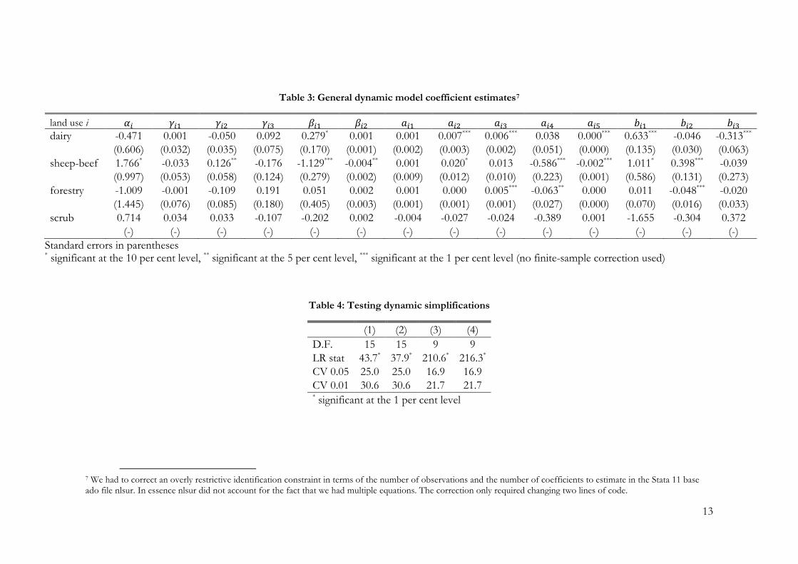
6.1. Estimation of the general dynamic model
We estimate the general dynamic model in equation ( 10 ) using feasible iterated
generalised least squares. Our results are presented in Table 3. For the 𝑖-th land share 𝛼𝑖 is the
estimated long run constant, 𝛾𝑖𝑗 is the estimated long run coefficient of the 𝑗-th price, 𝛽𝑖1 is the
long run effect of exogenous changes in other land, and 𝛽𝑖2 is the long run effect of interest rates.
𝑎𝑖𝑗 is the short run effect of the 𝑗-th price for 𝑗 ∈ {1, 2, 3}, the short run effect of changes in
other land for 𝑗 = 4 , and the short run effect of interest rates for 𝑗 = 5 . 𝑏𝑖𝑗 represent the
composite adjustment factors – recall that individual adjustment factors are not identified.
Standard errors are presented in parentheses. These are too small in finite samples.
However given the amount of data we are working with there are relatively few statistically
significant estimates in any case. We have not implemented finite sample corrections.
13
Table 3: General dynamic model coefficient estimates7
land use i
𝛼𝑖 𝛾𝑖1 𝛾𝑖2 𝛾𝑖3 𝛽𝑖1 𝛽𝑖2 𝑎𝑖1 𝑎𝑖2 𝑎𝑖3 𝑎𝑖4 𝑎𝑖5 𝑏𝑖1 𝑏𝑖2 𝑏𝑖3 dairy -0.471 0.001 -0.050 0.092 0.279* 0.001 0.001 0.007*** 0.006*** 0.038 0.000*** 0.633*** -0.046 -0.313***
(0.606) (0.032) (0.035) (0.075) (0.170) (0.001) (0.002) (0.003) (0.002) (0.051) (0.000) (0.135) (0.030) (0.063) sheep-beef 1.766* -0.033 0.126** -0.176 -1.129*** -0.004** 0.001 0.020* 0.013 -0.586*** -0.002*** 1.011* 0.398*** -0.039
(0.997) (0.053) (0.058) (0.124) (0.279) (0.002) (0.009) (0.012) (0.010) (0.223) (0.001) (0.586) (0.131) (0.273) forestry -1.009 -0.001 -0.109 0.191 0.051 0.002 0.001 0.000 0.005*** -0.063** 0.000 0.011 -0.048*** -0.020
(1.445) (0.076) (0.085) (0.180) (0.405) (0.003) (0.001) (0.001) (0.001) (0.027) (0.000) (0.070) (0.016) (0.033) scrub 0.714 0.034 0.033 -0.107 -0.202 0.002 -0.004 -0.027 -0.024 -0.389 0.001 -1.655 -0.304 0.372
(-) (-) (-) (-) (-) (-) (-) (-) (-) (-) (-) (-) (-) (-) Standard errors in parentheses * significant at the 10 per cent level, ** significant at the 5 per cent level, *** significant at the 1 per cent level (no finite-sample correction used)
Table 4: Testing dynamic simplifications
(1) (2) (3) (4) D.F. 15 15 9 9 LR stat 43.7* 37.9* 210.6* 216.3*
CV 0.05 25.0 25.0 16.9 16.9 CV 0.01 30.6 30.6 21.7 21.7 * significant at the 1 per cent level
7 We had to correct an overly restrictive identification constraint in terms of the number of observations and the number of coefficients to estimate in the Stata 11 base ado file nlsur. In essence nlsur did not account for the fact that we had multiple equations. The correction only required changing two lines of code.

14
Looking at the long run price responsiveness we see that most shares are estimated to
increase as their own commodity price increases but to decrease as competing commodity prices
increase. There are three exceptions, which from the point of view of simulating scenarios are
important: the dairy share is positively associated with forestry prices; the scrub share is
positively associated with dairy prices; the scrub share is positively associated with sheep-beef
prices. The dairy share, forestry price, association is something that comes through strongly in
the data. We do not think this represents a causal relationship. However we are not sure why
these two time series historically have happened to have a high degree of linear co-movement –
not that the land shares on the left hand side are already differenced. The scrub share,
commodity price relationships are also unusual. These exceptions should remind us that we are
not estimating causal relationships, and thus we must use judgement and care when producing
scenarios based on New Zealand’s national land use data.
The short run price relationships are also interesting. The change in land share for all
productive uses is estimated to increases as any commodity price increases (in fact the forestry
share has a negative coefficient if it is shown to 4 decimal places). All changes in commodity
prices are estimated to have negative coefficients in the scrub share equation. Thus there appears
to be a split in the short run between productive and unproductive use. This could suggest an
important omitted variable, such as GDP, or exchange rates, which could be important in
allowing changing land use in the short run – perhaps due to facilitating access to credit.
However we report results including real GDP and the UK exchange rate both separately and
together in the appendix and our results do not change qualitatively8
6.2. Testing dynamic simplifications
.
The dynamic specification of our model is likely to be important because land use
choices now affect future land use profitability. Several simpler dynamic structures are nested in
our general model and can be implemented by appropriate coefficient restraints. In particular
Anderson and Blundell (1982), (1983) showed the coefficient restrictions necessary to collapse
the general model to either an AR(1) model, a partial adjustment model, or a static model.
Consider equation ( 10 ): if each 𝑎𝑖𝑗 = 𝜋𝑖𝑗 for all 𝑖 and 𝑗 then we get the AR(1) model; if each
𝑎𝑖𝑗 = ∑ 𝑏𝑖𝑘3𝑘=1 𝜋𝑘𝑗 we get the partial adjustment model; from either the AR(1) model or the
partial adjustment model we can get the static model by constraining 𝑏𝑖𝑗 = 𝛿𝑖𝑗 where 𝛿𝑖𝑗 is the
kronecker delta.
8 Exchange rate data is obtained from the Reserve Bank of New Zealand’s website – the Trade Weighted Index does not extend back as far as our data series, so we use the UK exchange rate.

15
We test each of these dynamic simplifications in turn using likelihood ratio tests. Our
results are presented in Table 4. The D.F. row reports the number of coefficient constraints
necessary to implement the nested model. The LR stat row reports the likelihood ratio statistic
for the test. CV 0.05 and CV 0.01 report the 𝜒𝐷.𝐹.2 critical value for D.F. degrees of freedom at
the 5 per cent and 1 per cent levels respectively. Column (1) reports the test for the general
model against the AR(1) model; column (2) gives results for the general model against the partial
adjustment model. The static model is tested against the AR(1) model and the partial adjustment
model in columns (3) and (4). All simplifications can be rejected at the 1 per cent level. The most
general model we consider, which allows the disequilibrium in dairy, sheep-beef, and forestry to
affect all land use changes is always preferred in our data.
7. Baseline scenario
In this section we present a baseline scenario for land use until 2050. For this scenario we
use the price projections used in MAF’s Pastoral Supply Response Model until 2015 (using
lagged prices as our predictors these have effects until 2016). From 2015 onward we assume
constant real prices. We also assume that nominal interest rates and the share of land that is not
in any of the four major rural uses stays constant at its 2008 level going into the future. Under
these assumptions our baseline scenario is shown in Figure 4.
Figure 4: Baseline scenario, 2009-2050
0.2
.4.6
.81
Sha
re o
f rur
al la
nd
1975 1985 1995 2005 2015 2025 2035 2045Year
dairy share sheep-beef shareforestry share scrub share

16
The vertical grey line separates the graph into two sections. The left side shows observed
land share data from 1974-2008. The right hand side shows our baseline projections when there
is no NZ ETS. We have smoothed the dynamics in the first 10 years – there was some
fluctuation as changing projected prices affected long run equilibrium levels. The two important
aspects of the baseline scenario are its overall trends, and its dynamics. These are both driven by
changes in projected prices, because these are the only predictors which vary between 2009 and
2050. In particular the real dairy price projections increase from 635 to 937 cents per kilogram of
milk solids, the sheep-beef price projections increase from 533 to 549 cents per kilogram, while
the forestry price increases from 11970 to 19288 cents per cubic metre of wood. Until 2016
these price projections result in relative price changes – however from 2017 onwards all relative
prices are stable.
The change in projected forestry prices dominates the other changes in terms of its
magnitude. Thus, because the long run forestry share increases with the forestry price, and the
long run sheep-beef and scrub shares fall with forestry prices it is not surprising that the long run
trend is for increasing forestry and decreasing sheep-beef and scrub. The long run dairy trend
should be assessed with care. In particular our estimates show that the dairy share responds
positively to increases in forestry prices. We do not think that this represents a causal effect –
however the correlation appears strongly in historic New Zealand land use data. This
responsiveness results in the dairy share increasing more in the baseline than it would if it were
only being driven by increases in the dairy price projections.
Our current baseline has rather volatile short run dynamics. These mainly show up in the
sheep-beef and scrub shares which have the quickest aggregate responses to disequilibrium
effect.9
8. Conclusion
These are due to swings in relative commodity prices over the period in which price
projections are variable. Once relative commodity prices projections settle down these dynamics
no longer have an important role.
This paper has estimated the relationships between New Zealand’s main rural land uses
and their associated export prices using national time series data. We have a short time series and
so it is not surprising that many of our coefficient estimates are not statistically significant.
In the short run we estimate that most productive land uses are positively associated with
relevant prices, while unproductive scrub is negatively associated with relevant prices. In the long
9 Recall that the individual adjustment factors are not identified.

17
run all land shares were estimated as being positively associated with the price of their own
products and most were estimated to have a negative relationship with the price of products
from other land uses.
Theoretically we think that dynamic considerations should be important for land use
choices. This hypothesis is reinforced by the data. Likelihood ratio tests overwhelmingly reject
the static models in favour of the simple dynamic AR(1) and partial adjustment models.
Furthermore both of these models are rejected at the 1 per cent level compared to our more
general model.
For simulation work there are further limitations that should be kept in mind. We have
time series data from before the implementation of the NZ ETS. Our estimates of land use
responsiveness to economic returns are based on this data and we have not allowed for
structural change – in particular the ETS itself may represent a structural change. Furthermore
simulations based on our parameter estimates must explicitly incorporate the structure of
expectations of future returns. Because of conversion costs land use may not respond to changes
in economic returns that are perceived as purely transitory.
This work represents are first step in estimating how rural land use responds to
economic factors in New Zealand. Further work will continue to explore the relationship
between rural land use and economic returns using panel data provided by Statistics New
Zealand at a Territorial Local Authority level, as well as satellite and land use panel data in 1996,
2002, and 2008. This collection of work will help estimate the impact of policy that aims to
achieve environmental outcomes by changing land use through affecting economic incentives.
References
Anderson, G. J. and R. W. Blundell. 1982. "Estimation and Hypothesis Testing in Dynamic Singular Equation Systems", Econometrica, 50:6, pp. 1559-71.
Anderson, Gordon and Richard Blundell. 1983. "Testing Restrictions in a Flexible Dynamic Demand System: An Application to Consumers' Expenditure in Canada", Review of Economic Studies, 50:3, pp. 397-410.
Anderson, Kym; Ralph Lattimore; Peter Lloyd and Donald Maclaren. 2007. "Distortions to Agricultural Incentives in Australia and New Zealand," World Bank Agricultural Distortions Working Paper 09.
Choi, In. 2001. "Unit Root Tests for Panel Data", Journal of International Money and Finance, 20:2, pp. 249-72.

18
Deaton, Angus and John Muellbauer. 1980. "An Almost Ideal Demand System", American Economic Review, 70:3, pp. 312-26.
Hadri, Kaddour. 2000. "Testing for Stationarity in Heterogenous Panel Data", Econometrics Journal, 3, pp. 148-61.
Miller, Douglas J. and Andrew J. Plantinga. 1999. "Modelling Land Use Decisions With Aggregate Data", American Journal of Agricultural Economics, 81:1, pp. 180-94.
Ng, Serena. 1995. "Testing for Homogeneity in Demand Systems When the Regressors Are Nonstationary", Journal of Applied Econometrics, 10:2, pp. 147-63.
Parks, Peter J. 1995. "Explaining Irrational Land Use: Risk Aversion and Marginal Agricultural Land", Journal of Environmental Economics and Management, 28:1, pp. 34-47.
Stavins, Robert N. and Adam B. Jaffe. 1990. "Unintended Impacts of Public Investments on Private Decisions: The Depletion of Forested Wetlands", American Economic Review, 80:3, pp. 337-52.
Appendix A
In this appendix we present two sets of estimation results that include separately GDP
and the UK exchange rate. Inclusion of GDP and the UK exchange rate together yields
qualitatively similar results.
Our motivation for including these explanatory variables is the interesting short run
coefficients in our preferred specification. In particular almost all shares responded positively to
increases in any price. One possible explanation for this result could be that planned conversions
are undertaken when the economy is doing well and land managers are not so credit constrained.
The results from these specifications are presented in Table 5 and Table 6.
Both sets of coefficient estimates are similar to each other, and to our preferred
specification reported in Table 3. Importantly the split between short run productive and
unproductive land use responses to commodity prices is still apparent. Thus, so far, we are
unable to explain what is driving our estimated short run coefficients. This will be of interest in
future research on land use using other data sets.

19
Table 5: General dynamic model with GDP included
land use i 𝛼𝑖 𝛾𝑖1 𝛾𝑖2 𝛾𝑖3 𝛽𝑖1 𝛽𝑖2 𝛽𝑖3 𝑎𝑖1 𝑎𝑖2 𝑎𝑖3 𝑎𝑖4 𝑎𝑖5 𝑎𝑖6 𝑏𝑖1 𝑏𝑖2 𝑏𝑖3 dairy -0.504 0.000 -0.009 0.067 0.066 0.000 0.004 0.001 0.006 0.006 0.016 0.000 0.003 0.556 -0.060 -0.264 0.587 0.017 0.031 0.070 0.259 0.001 0.002 0.002 0.004 0.002 0.054 0.000 0.001 0.132 0.029 0.072 sheep-beef 2.386 -0.026 0.095 -0.223 -1.201 -0.005 -0.003 0.002 0.039 0.011 -0.770 -0.002 -0.002 0.863 0.374 0.257 1.849 0.055 0.097 0.221 0.815 0.005 0.008 0.008 0.017 0.009 0.241 0.001 0.006 0.588 0.130 0.321 forestry -1.464 -0.008 -0.022 0.179 -0.257 0.000 0.009 0.001 0.000 0.005 -0.059 0.000 -0.001 0.029 -0.044 -0.030 1.786 0.053 0.094 0.213 0.787 0.005 0.008 0.001 0.002 0.001 0.030 0.000 0.001 0.073 0.016 0.040 scrub 0.582 0.033 -0.083 0.111 -0.457 0.004 -0.001 -0.002 -0.033 -0.010 -0.187 0.002 0.005 -0.335 -0.390 -0.491 (-) (-) (-) (-) (-) (-) (-) (-) (-) (-) (-) (-) (-) (-) (-) (-)
Standard errors in parentheses * significant at the 10 per cent level, ** significant at the 5 per cent level, *** significant at the 1 per cent level (no finite-sample correction used)
Table 6: General dynamic model with UK exchange rates included
land use i 𝛼𝑖 𝛾𝑖1 𝛾𝑖2 𝛾𝑖3 𝛽𝑖1 𝛽𝑖2 𝛽𝑖3 𝑎𝑖1 𝑎𝑖2 𝑎𝑖3 𝑎𝑖4 𝑎𝑖5 𝑎𝑖6 𝑏𝑖1 𝑏𝑖2 𝑏𝑖3 dairy -0.284 0.001 -0.045 0.070 0.236 0.001 -0.016 0.001 0.009 0.007 0.018 0.000 0.006 0.702 -0.038 -0.400 0.440 0.026 0.038 0.059 0.169 0.001 0.062 0.002 0.003 0.002 0.050 0.000 0.008 0.133 0.029 0.077 sheep-beef 1.534 -0.033 0.123 -0.150 -1.062 -0.004 0.014 0.001 0.015 0.011 -0.547 -0.001 0.030 0.890 0.370 0.041 0.787 0.047 0.067 0.106 0.303 0.003 0.111 0.008 0.012 0.010 0.221 0.001 0.035 0.591 0.129 0.340 forestry -0.487 0.000 -0.085 0.121 -0.005 0.001 -0.069 0.001 -0.001 0.004 -0.061 0.000 0.003 0.008 -0.049 -0.022 0.895 0.054 0.077 0.121 0.344 0.003 0.126 0.001 0.001 0.001 0.027 0.000 0.004 0.072 0.016 0.042 scrub 0.237 0.035 -0.083 0.098 -0.169 0.004 0.038 0.000 -0.005 -0.008 -0.410 0.001 -0.027 -0.197 -0.359 -0.419 (-) (-) (-) (-) (-) (-) (-) (-) (-) (-) (-) (-) (-) (-) (-) (-)
Standard errors in parentheses * significant at the 10 per cent level, ** significant at the 5 per cent level, *** significant at the 1 per cent level (no finite-sample correction used)