Modelling Gasoline Demand in the United States: A Flexible

Semiparametric Approach

Weiwei Liu∗

Department of Economics

State University of New York at Binghamton

August 4, 2011

Abstract

Using the most recently available data, this paper estimates the price and income elasticities of

gasoline demand in the United States from a semiparametric smooth coefficient model. The econo-

metric approach provides more flexibility by allowing functional coefficients to accommodate hetero-

geneity in gasoline demand. Instrumental variables are used to correct for the potential endogeneity

of the price of gasoline that has often been ignored in the literature. A formal model specification

test rejects the parametric translog model, and suggests strong evidence of heterogeneous gasoline

demand across states and over time. The results illustrate a significant income effect and price ef-

fect on gasoline demand elasticities. The dynamics of the gasoline price is the driving force behind

the time variation of elasticities, and the demand for gasoline is more sensitive to unpredicted price

shocks than gradual fluctuations. State level attributes, such as government expenditure on public

transportation, contribute to the cross-state variation in gasoline demand elasticities.

JEL Classification: C14, Q41, Q54.

Keywords: Gasoline demand, elasticity, semiparametric estimation.

∗Correspondence to: Weiwei Liu, Department of Economics, State University of New York, Binghamton, NY 13902-6000.Phone: 607-777-2572, Fax: 607-777-2681, E-mail: wliu5@binghamton.edu.

1

1 Introduction

In most countries, carbon dioxide (CO2) forms the largest proportion of greenhouse gas

emissions, and is considered to be the major cause of global warming (United Nations

Framework Convention on Climate Change). In the United States, 85% of the total

emissions of greenhouse gases is carbon dioxide, 33.8% of which is derived from the trans-

portation sector.1 Besides environmental regulations, imposing a gasoline tax is one way

to reduce the gasoline consumption and greenhouse gas emissions in the transportation

sector. The effectiveness of such a tax largely depends on how gasoline demand responds

to price changes, the measurement of which calls for a properly specified demand model

and precise estimation of the price elasticity.

Gasoline demand has been widely studied in the last 30 years. After the negotiation of

the Kyoto Protocol in 1997, concerns about increasing greenhouse gas emissions and global

warming have renewed interest in understanding gasoline demand in the last decade. A

reduced-form demand model applied to aggregate data to estimate the demand for gasoline

has been, by far, the most preferred and dominant approach in both the academic and

non-academic literature. Hundreds of studies have been conducted to assess the price

elasticity and income elasticity of gasoline consumption at country or region levels. There

are also a great number of reviews and surveys attempting to synthesize and compare the

results of those studies (e.g., Drollas 1984, Blum 1988, Dahl and Sterner 1991, Goodwin

1992, Sterner and Dahl 1992, Dahl 1995, Espey 1998, Graham and Glaister 2002, Goodwin

et al. 2004, Basso and Oum 2007). However, the magnitude of the elasticities found in

the literature varies substantially, which Baltagi and Griffin (1983) believe is caused by

differences in methodologies and data. Goodwin (1992), on the other hand, shows that

data type, i.e., cross-section or time-series, only marginally affects the magnitude of the

estimated elasticities.

Another possible explanation for the broad range of estimated gasoline demand elas-

ticities is that they are not constant. There exists a fairly diverse set of empirical studies

investigating this issue, but unfortunately, the literature has yielded mixed results. Dahl

(1982) first investigates whether gasoline demand elasticities change over time in the con-

text of the oil crisis in 1973. A series of Chow tests indicate that the price and income

elasticities do not vary with respect to severe price fluctuations, nor do the elasticities vary

with income. Dahl (1995) reports different results after reviewing a number of gasoline

demand studies for the U.S., and concludes that overall the gasoline demand elasticities

tend to decrease over time. On the contrary, based on a comparison of the works in the

1980s and 1990s with previous studies, Goodwin (1992) shows that the magnitude of the

estimated elasticities has been slightly going up.

1Source: U.S. Energy Information Administration, Emissions of Greenhouse Gases Report, 2009.

2

Gasoline demand elasticities may also vary with the widely changing price and in-

come. Although Goodwin et al. (2004) present a mathematical derivation that the price

elasticity is negatively related to income, the exact relation still remains ambiguous. The

popular log-linear model which gives constant elasticities is unable to answer this ques-

tion. A translog model on the other hand is preferred in this case, as the inclusion of

the quadratic and interaction terms allows the elasticities to vary with different price and

income levels. Using the translog specification and household level data, Archibald and

Gillingham (1980) find that both the price and income elasticities are higher for low in-

come households; Hausman and Newey (1995) find that the price elasticity is not affected

by income but varies with price; in Kayser (2000), the income elasticity falls with higher

incomes, but the price elasticity increases with higher incomes; while in Wadud et al.

(2010a) both the price elasticity and income elasticity increase as income increases.

Since no guidance is provided by economic theory regarding the appropriate gasoline

demand model, recent studies have explored more flexible functional forms. Using a

semiparametric partially linear model, Hausman and Newey (1995) find evidence of a

nonlinear demand, which confirms the necessity of using flexible functional forms for the

estimation of gasoline demand model. Following the similar technique, Schmalensee and

Stoker (1999) find no evidence that income elasticity decreases as income increases, while

Wadud et al. (2010b) find a “U” shaped pattern for the price elasticity and a slightly

decreasing trend for the income elasticity as income increases.

This paper has three major contributions to the empirical literature on gasoline de-

mand. First, a semiparametric smooth coefficient model is used to incorporate parameter

heterogeneity and obtain observation specific estimates of the price elasticity and income

elasticity. This specification is able to address some questions that are not clearly an-

swered by previous studies, such as how personal income and the gasoline price affect

the price and income elasticities of gasoline demand, whether the elasticities change over

time, and whether or not other factors induce heterogeneity. Second, a model specification

test is conducted to verify the robustness of the semiparametric demand model against

the parametric translog demand model. Third, examines the endogeneity of the price of

gasoline which has often been ignored in literature, and obtains consistent estimates using

carefully selected instruments. Moreover, various models without instrumental variables

are also estimated to assess the sensitivity of the regression results to the selection of

instruments.

The primary results are consistent with previous studies in that the demand for gaso-

line in the U.S. is overall inelastic. In addition, this paper finds significant evidence

of parameter heterogeneity using the semiparametric demand model. More specifically,

personal income and the gasoline price have shown substantial impacts on demand elas-

3

ticities. The demand elasticities not only vary across states, but also change over time,

which is mainly driven by the fluctuation in the gasoline price. The demand for gasoline

is more sensitive to abrupt and dramatic price shocks than gradual changes. State level

attributes, such as the average fuel efficiency of vehicles and the availability of public

transportation, also affect the elasticities of gasoline demand.

In order to assess the robustness of the primary results, I conduct a bootstrap proce-

dure to test the smooth coefficient model against the null hypothesis of the parametric

translog model. The test shows that the semiparametric gasoline demand model is pre-

ferred to the traditional translog model. That is, the model specification test confirms

the result that gasoline demand elasticities not only vary with different income and price

levels, but also display significant heterogeneity across states and over time. When re-

moving the instrumental variables used for the gasoline price, the estimates are slightly

biased downward implying the validity of the selected instruments and the existence of

endogeneity.

The remainder of the paper is organized as follows. Section 2 introduces the semi-

parametric smooth coefficient method for the estimation of gasoline demand, followed by

the description of the data in Section 3. Section 4 presents the estimation results for

both parametric and semiparametric models along with a detailed discussion. Section 5

and 6 provide model specification testing and sensitivity analyses, and finally Section 7

concludes.

2 Methodology

2.1 Model specification

Following previous literature (Archibald and Gillingham 1980, Hausman and Newey 1995),

I consider the translog model to be the baseline model structure, where gasoline demand

is a function of the price of gasoline, income, their quadratic and interaction terms, and

other dummy variables

lnGit = β0 + βP lnPit + βY lnYit + βPP (lnPit)2 + βY Y (lnYit)

2 + βPY lnPit lnYit

+ β1Q1it + β2Q2it + β3Q3it + β4NEi + β5MWi + β6Si + ui + εit, (1)

where

Git is the gasoline consumption per capita in state i at time t,

Pit is the price of gasoline in state i at time t,

Yit is the disposable income per capita in state i at time t,

Q1it, Q2it and Q3it are quarter dummies,

4

NE, MW and S are regional dummies for Northeast, Midwest and South,

ui is the unobserved state effect,

and εit is the i.i.d. error term.

The price and income elasticities of gasoline demand (peit and ieit respectively) can be

derived from the model as

peit =∂ lnGit

∂ lnPit= βP + βPY lnYit + 2βPP lnPit;

ieit =∂ lnGit

∂ lnYit= βY + βPY lnPit + 2βY Y lnYit. (2)

Unlike the log-linear model, the translog model provides more flexibility for the in-

clusion of the quadratic and interaction terms, which capture the heterogeneity in the

elasticities across different income and price levels. The effects of income and price are

determined by the sign and magnitude of the coefficients. For example, as income in-

creases, a positive value of βPY indicates a decrease in the absolute price elasticity, and a

positive value of βY Y indicates an increase in the income elasticity. The translog specifi-

cation allows the demand elasticities to vary with income and price in a relatively flexible

manner. It also implicitly assumes that income and price are the only sources of elasticity

heterogeneity, and the demand elasticities are strictly linearly related to both income and

price. However, except for price and income, other factors are also likely to affect the

sensitivity of gasoline demand in a particular area, such as the availability of public tran-

sit, average fuel efficiency, and the population density. Moreover, the demand elasticities

may not be simple linear functions of price, income, or any other explanatory variable,

therefore a more flexible functional form is necessary (Hausman and Newey 1995).

In order to sufficiently capture the heterogeneity in gasoline demand elasticities, I use

the following semiparametric smooth coefficient model2

lnGit = β0(Zit) + βP (Zit) lnPit + βY (Zit) lnYit + βPP (Zit)(lnPit)2 + βY Y (Zit)(lnYit)

2

+ βPY (Zit) lnPit lnYit + β1(Zit)Q1it + β2(Zit)Q2it + β3(Zit)Q3it

+ β4(Zit)NEi + β5(Zit)MWi + β6(Zit)Si + εit, (3)

where Zit is a vector of attribute variables that not only directly affect the consumption

of gasoline, but also influence the responsiveness of gasoline demand. The price elasticity

2To ensure the the comparability with model (1), a state indicator is included in the coefficient functions to control theunobserved state effect.

5

and income elasticity are thus functions of price, income and all the attribute variables

peit =∂ lnGit

∂ lnPit= βP (Zit) + βPY (Zit) lnYit + 2βPP (Zit) lnPit;

ieit =∂ lnGit

∂ lnYit= βY (Zit) + βPY (Zit) lnPit + 2βY Y (Zit) lnYit. (4)

The semiparametric model relaxes the constant parameter assumption, and allows all

the coefficients to be unknown smooth functions of the attribute variables (Zit). The

shortcoming of using the conventional log-linear or translog model to estimate gasoline

demand is that they implicitly assume all observations have exactly the same demand

structure and constant coefficients may only be obtained. Therefore, they may not be

able to accurately identify the differences in demand among observations that may be

crucial for understanding the behavior of gasoline consumption in different states and

different time periods. There are three advantages of the varying coefficient model as

specified in equation (3). First, unlike a fully nonparametric regression without any

functional form assumptions, it maintains the basic translog demand structure. Second,

similar to the translog model, it obtains observation specific coefficients and elasticities

at different price and income levels, which allows one to investigate the price and income

effects on gasoline consumption. Third, the functional coefficients are flexible enough

to incorporate parameter heterogeneity caused by factors other than income and gasoline

price, and possibly identify the source of heterogeneity by selecting appropriate state level

attribute variables.

2.2 NPGMM estimation

Model (3) can be generalized as

Yit = X ′itg(Zit) + εit (5)

where X it is a vector of regressors, and the coefficient functions g(·) are unspecified

smooth functions of a vector of variables Zit. Of particular interest is the estimation of the

functional coefficients g(·). A nonparametric generalized method of moments (NPGMM)

approach, proposed by Cai and Li (2008), is considered here. They impose conditional

moment restrictions similar to the GMM estimation of Hansen (1982) and apply the

local-linear fitting scheme of Fan and Gijbels (1996) to estimate the functional coefficients.

Hence the NPGMM procedure is a combination of the above two techniques. The detailed

description of this approach and the estimator can be found in Cai and Li (2008).

It is well known that smoothing parameter (bandwidth) selection plays an important

role in the estimation of nonparametric and semiparametric kernel models. This is espe-

6

cially true in multidimensional problems. Data-driven methods are preferred due to their

desirable properties, such as converging to the optimal bandwidths as the sample size

grows. I will particularly use least-squares cross-validation to select the bandwidths. The

advantage of this selection procedure over other methods is its ability to detect if a dis-

crete variable is relevant and remove the irrelevant ones automatically. For instance, if the

estimated smoothing parameter for a discrete variable is equal to unity (the bandwidth

upper bound for discrete variables assuming the Racine and Li (2004) kernel functions),

all observations will be assigned the same weight by the kernel function. In this case,

the discrete variable is irrelevant. For a continuous variable, a bandwidth above the up-

per bound means that variable enters the function linearly. Therefore, the least-squares

cross-validation method can easily eliminate the irrelevant discrete variables and identify

a correct relation (linear or nonlinear) with continuous variables as long as it provides the

best fit to the data. For more information on data driven bandwidth selection, see Li and

Racine (2007).

2.3 Endogeneity and IV selection

The price of gasoline is usually considered exogenous in the literature (Archibald and

Gillingham 1980, Hausman and Newey 1995, Schmalensee and Stoker 1999, Wadud et

al. 2010a and 2010b), because these authors believe that the gasoline price is mainly

determined by the crude oil price in the world market instead of by demand. However,

simply regressing demand on price will inevitably cause a correlation with the error term,

since the quantity demanded and the price are determined simultaneously, especially

when the U.S. is the largest crude oil consumer in the world. In this circumstance, the

estimates will likely be biased and inconsistent. An ideal instrumental variable should be

both correlated with the endogenous regressors and orthogonal to the errors, but finding

an appropriate instrument for the price of gasoline has proved to be extremely difficult in

the literature.

Ramsey et al. (1975) and Dahl (1979) use the relative prices of other petroleum

products such as kerosene and residual fuel oil as instrumental variables. The validity

of this instrument is arguable, because the prices of those refinery outputs are likely to

be correlated with gasoline demand shocks through the price of crude oil. Both Yachew

and No (2001) and Manzan and Zerom (2010) fail to reject the null hypothesis that price

is exogenous when using regional dummy variables as instruments. The problem is that

regional dummies may correlate with gasoline consumption due to differences in land use

patterns, the density of development and the size of each state. Hughes et al. (2008)

consider crude oil production disruptions of three oil producing countries as instrumental

variables, but that data is available only at the country level, which is not suitable for

7

this state level study.

If the price of gasoline is mostly determined by the world crude oil market, the gaso-

line price in different states during the same period should be correlated, which implies

theoretically that the gasoline price in one state could be instrumented by the price in

another. Empirically there is no unique standard to choose the price of one state as an

instrument over another, because many factors could be considered, such as the physical

distances, similarity in weather conditions, etc. To avoid complexity, I take the average

price of all other non-adjoining states to instrument the price variable of a particular

state. For example, New York state neighbors Vermont, Massachusetts, Connecticut,

New Jersey, and Pennsylvania, so the instrumental variable for the gasoline price in New

York is the average price in all states except New York, Vermont, Massachusetts, Con-

necticut, New Jersey, and Pennsylvania. The correlation between instrumental variables

and endogenous regressors can be assessed by looking at the significance of a first stage

instrumental variables (IV) regression. A sufficiently high F-statistic implies the relevance

of the selected instrumental variables (Staiger and Stock 1997).

3 Data

The data set spans the period 1994 to 2008, and is in quarterly intervals. Gasoline con-

sumption is approximated as monthly “prime supplier sales volumes of motor gasoline”,

per capita per day, obtained from the U.S. Energy Information Administration (2009).

The after tax gasoline prices are computed by adding the state/federal tax rates (U.S.

Department of Transportation, Highway Statistics) to the “motor gasoline sales to end

user price” (U.S. Energy Information Administration, 2009). Quarterly personal dispos-

able income is collected from the U.S. Bureau of Economic Analysis, Regional Economic

Accounts (2009). Since monthly tax and income data at the state level are not available,

gasoline prices and consumption are converted to quarterly data for convenience. Prices,

income, and tax rates are converted to constant 2005 dollars using GDP implicit price de-

flators obtained from the Bureau of Economic Analysis (2009). The District of Columbia

is excluded due to the presence of too many missing values. In total there are 50 states

and 60 periods (3000 observations) in the sample. Summary statistics of the variables

and data are presented in Table 1.

A number of attribute variables that enter the coefficient functions are used to inves-

tigate the potential heterogeneity of gasoline demand elasticities. These variables include

two discrete variables indicating “state id” and “year”, and three continuous variables: the

cumulated public transit expenditure by state and local government (U.S. Department of

Transportation, Bureau of Transportation Statistics, Government Transportation Finan-

8

cial Statistics 1995-2007), the ratio of trucks3 to the total number of vehicles on the road

(U.S. Department of Transportation, Highway Statistics), and the ratio of urban popu-

lation to the state total population (U.S. Bureau of the Census). Expenditure on public

transit is used to approximate the availability of public transportation. Fuel efficiency

(measured in miles per gallon) for passenger cars (22.6 mpg) is much higher than light

trucks (18.1 mpg), hence the ratio of trucks can indicate the average fuel efficiency.4 The

ratio of urban population may capture the difference in gasoline demand elasticities in

the states with a larger urban population relative to those with a larger rural population.

4 Results

Table 2 gives the results from the translog model and the semiparametric model with

and without instrumental variables. The random effect estimation is used for the baseline

parametric translog model. Parameter estimates for price and income are significant at

the 1% confidence level with the expected signs. The variables included in the smooth

coefficient functions, i.e. government expenditure on public transit, ratio of trucks, ratio

of urban population, and year, are considered as linear regressors in the trasnlog specifica-

tion. The coefficients of the former two variables are significant at a 5% confidence level,

implying that the average gasoline consumption in a state is significantly affected by the

government expenditure on public transit and the ratio of trucks. No sufficient difference

in average gasoline consumption is observed in the states with larger urban population

relative to the others, given the insignificant coefficient on urban population ratio. For

the purpose of comparison, the mean of the semiparametric smooth coefficients are also

reported in the table.5

One appealing advantage of the smooth coefficient model over the translog model is

that, instead of a constant coefficient, it estimates a smooth coefficient function on each

regressor to capture the potential heterogeneity. This is important for the investigation of

elasticity heterogeneity, because some coefficients (e.g. βP , βY , βPY , βPP , and βY Y ) are

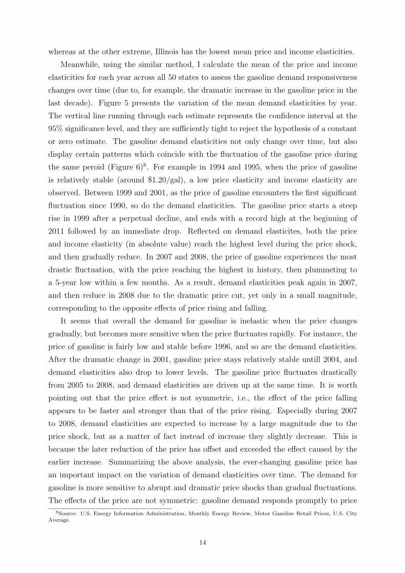
the crucial factors that determine demand elasticities. Figure 1 plots the kernel densities of

these coefficients and the constant estimates from the translog model. The vertical line in

each panel represents the coefficient from the translog model. Compared with distribution

estimates, the constant coefficients not only lack flexibility, but are also strongly biased.

The observation specific price and income elasticities are computed based on equations

(2) and (4) for the translog model and the semiparametric smooth coefficient model re-

spectively. The mean elasticity for each model is reported in Table 2. For price elasticity,

3Trucks include vans, pickup trucks, sport utility vehicles and other light trucks4Source: U.S. Energy Information Administration, Monthly Energy Review.5The median coefficients provide quantitively similar resultes.

9

the mean estimates obtained from the two models are slightly different, but the small

magnitude suggests that the gasoline demand in the United States is overall insensitive

to price changes. The income elasticity on the other hand, shows more variation: the

mean value given by the semiparametric model is significantly smaller than its translog

counterpart.6 Since the variables selected in the two models are exactly the same, the only

factor that may cause different estimation results is model specification. The bootstrap

test presented in Section 5 rejects the parametric translog model in favor of the semipara-

metric smooth coefficient model, which also implies that ignoring coefficient heterogeneity

results in an overestimate of the income effect.

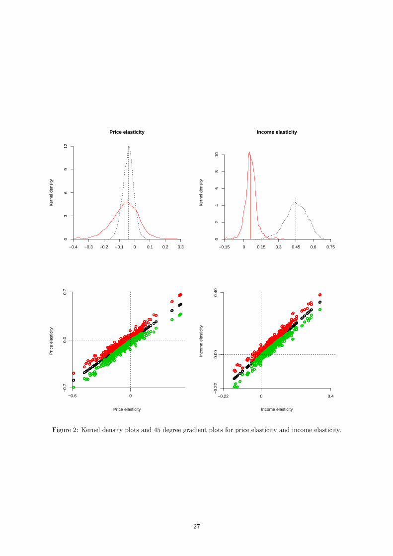
4.1 Density and significance analysis

Both the translog model and smooth coefficient model are able to obtain observation spe-

cific demand elasticities, hence one can plot the probability density functions to examine

the distributions of demand elasticities. The kernel density plots for the price elasticity

and income elasticity are shown in the top two panels of Figure 2. In each panel, the solid

curve and the dashed black one represent the density estimates from the smooth coefficient

model and the translog model respectively. Comparing the mean and the overall distri-

bution, the demand elasticities are biased upwards using the translog model, especially

for the income elasticity. The elasticity estimates from the smooth coefficient model are

symmetrically distributed and centered around the mean, shown by the vertical line, with

a standard deviation of 0.103 for the price elasticity and 0.051 for the income elasticity.

These density plots provide evidence for elasticity heterogeneity which is observed more

in the price elasticity relative to the income elasticity.

Kernel density plots are able to depict the parameter heterogeneity by showing the

smooth probability density distributions, but they fail to provide the significance level.

In order to accurately describe both statistical inferences, I use another graphical aid to

present the results: the 45 degree gradient plots with confidence bounds. The intuition

for the 45 degree gradient plot is straightforward. The estimated parameter for each

observation is placed on the 45 degree line. The corresponding confidence bounds are

plotted above and below that particular estimate. The density of the estimate can be

seen through the clustering of the plots (although less visible than kernel density plots).

An estimate is positive and significant if its upper bound and lower bound both fall in

the first quadrant, and negative and significant if, on the other hand, they both fall in the

third quadrant. All other estimates are statistically insignificant, because the horizontal

line at zero runs between upper bounds and lower bounds, i.e. those estimates are not

6Espey (1996) uses meta-analysis to analyze estimates of gasoline demand elasticities. For the studies using state leveldata, the mean price elasticity is found to be -0.38, and the mean income elasticity is 0.60. However, those studies coverthe time period from 1936 to 1986, hence they may not be comparable to recent studies.

10

statistically different from zero.

The bottom two panels of Figure 2 display the 45 degree gradient plots for demand

elasticities,7 in which 77.8% of the observations have a significant estimate of the price

elasticity, and 89.7% of the observations have a significant estimate of the income elastic-

ity. From the density plots one may notice that for some observations, the price elasticity

is found to be positive, and the income elasticity negative. However, examining those

observations using the 45 degree gradient plots, most of the observations with a positive

price elasticity or negative income elasticity are statistically insignificant, and the ones

that are significant repeatedly occur in the same states. For instance, more than 50% ob-

servations from Rhode Island and Montana have a positive and significant price elasticity;

about 30% of the observations from New York and Hawaii have a negative and significant

income elasticity. Meanwhile, very few observations from those states are found to give

intuitive estimates, i.e. a negative and significant price elasticity and a positive and sig-

nificant income elasticity. Such counterintuitive results suggest that there maybe other

relevant factors influencing the gasoline demand in these states that is not captured by the

variables included in the model. In order to solve this problem, more detailed information

on the demand for gasoline in these states is required.

4.2 Income effect and price effect

Under the translog specification, the effect of income on the price elasticity is determined

by the coefficient of the interaction term between price and income (βPY ), and that on

the income elasticity is determined by the coefficient of the quadratic income term (βY Y ).

The parameter estimates indicate that as income increases, the absolute value of the price

elasticity and the income elasticity both decrease. In other words, at higher income levels,

the demand for gasoline is less sensitive to both income changes and price changes, and

this is consistent with some empirical studies (Archibald and Gillingham, 1980; Wadud

et al. 2010a).

Since the smooth coefficient model gives more flexibility than parametric models, it

is convenient and more sensible to investigate the demand elasticities at different income

levels. Based on the distribution of income, I divide the whole sample into six quantile

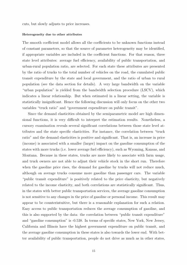
groups, and report the median price and income elasticity for each group. The results are

summarized in Table 3. The absolute value of the price elasticity increases incrementally

as income moves to higher quantiles. For the highest income quantile, the price elasticity is

-0.117, almost ten times bigger than that of the lowest income quantile in absolute value,

and sufficiently larger than other income quantiles. This implies that on average the

demand for gasoline in higher income groups is more elastic with respect to price. Using

7The standard errors of demand elasticities are estimated using a wild bootstrap.

11

household level data, Kayser (2000) draws a similar conclusion that households with lower

income do not respond as much to higher gasoline prices as wealthier households. The

explanation, which also applies to this study, is that people with low income are likely

to have already reduced their gasoline consumption to the minimal amount, leaving very

little room to respond noticeably to higher prices. Despite less incentive to respond to

higher gasoline prices, people with high income are more capable of adjustment such as

combining or reducing unnecessary trips. The variation of the median income elasticity

across quantile groups is inconspicuous, corresponding to the minor heterogeneity found

in the income elasticity using the full sample, but still showing a modest upward trend as

income increases. This suggests that income only slightly affects the income elasticity, and

the gasoline demand of the highest income group is relatively more sensitive to income.

Gasoline demand elasticities may also be influenced by different price levels, which is

reflected by the coefficients of the quadratic price term (βPP ) and the interaction term

(βPY ). The translog model yields a negative coefficient on the quadratic price term,

and the smooth coefficient model also finds a negative coefficient for most observations

as shown in Figure 1. This means that as the price of gasoline increases, the price

elasticity in absolute value also increases. Such a result is intuitive in that a higher gasoline

price raises the cost of driving and its expenditure share in total disposable income, in

which case people with relatively low income may reduce driving and hence gasoline

consumption. Therefore, a high price elasticity is expected when gasoline price reaches

a very high level. In addition, allowing heterogeneity in coefficient estimates enables

the semiparametric model to capture a more complicated relation. Similar to the above

analysis, I divide the whole sample into six quantile groups based on different price levels,

and also report the median price elasticity and income elasticity for each group. Unlike

the monotonic relationship with income, the absolute value of both the price and income

elasticity displays a “U” shaped variation as the price shifts to higher levels (see Table

3). The switching point occurs when the gasoline price is roughly around $1.30/gallon

(the price level before 2000). In other words, as the gasoline price increases, the demand

for gasoline becomes less sensitive to both price and income if the gasoline price is below

that level, but more sensitive when the gasoline price is above that level. Previous studies

do not provide consistent answers to this question. For example, Hausman and Newey

(1995) find no evidence of any effect; Kayser (2000) obtains a negative coefficient on the

interaction term, hence a lower income elasticity as the gasoline price rises; Wadud et al.

(2010a and 2010b) draw the opposite conclusion that the income elasticity will decrease

as the gasoline price rises.

Although the semiparametric smooth coefficient model reports a negative mean coeffi-

cient on the interaction term, positive on the quadratic income term, and negative on the

12

quadratic price term, it does not necessarily mean that income and price have exactly the

same effects for all the observations. This is also shown in Figure 1 where the magnitude

and sign of the coefficients are different for each observation. To take a closer look at

how income and price affect the elasticities of gasoline demand, I compute the observation

specific income and price partial effects obtained from the smooth coefficient model, and

bootstrap their standard errors for each observation. The kernel density plots of these

partial effects are presented in Figure 3. The top two panels are the income and price

partial effects on the price elasticity, and the bottom two panels are the income and price

partial effects on the income elasticity. The mean (absolute value) of the income partial

effect on the income elasticity and the price partial effect on the price elasticity are both

around 0.005, while the mean (absolute value) of the income partial effect on the price

elasticity and the price partial effect on the income elasticity are around 0.002. Hence, in

terms of magnitude, income has a stronger impact on the income elasticity, and the price

has a stronger impact on the price elasticity. As for the direction of those effects, 62.3% of

the observations have a negative and significant income effect on the price elasticity, and

more than 80% have a positive and significant income effect on the income elasticity. The

rest of the observations are mostly from Rhode Island, Montana, Hawaii, and New York,

which implies that in most of the states except the ones listed above, the demand for

gasoline gets more sensitive to both price and income with an increase in income. A neg-

ative and significant price partial effect is found for 65% of the observations on both the

price and income elasticity. The positive and significant price partial effect occurs mostly

before 2000 when the price of gasoline is relatively low (below $1.30/gallon). Therefore

in most cases, when the price of gasoline reaches a certain level, the gasoline demand

becomes more elastic with respect to price and less elastic with respect to income.

4.3 Heterogeneity in demand elasticities

Variation across states and over time

To analyze the difference in gasoline demand responsiveness across states, I average the

price and income elasticity for each state over the study period, and report the mean

elasticities in descending order as show in Table 4. Figure 4 displays these estimates

along with their confidence bounds. For both the price elasticity and income elasticity,

the mean estimates for most states are significant at the 95% significance level, which is

strong evidence of elasticity heterogeneity across states. Counterintuitive results are found

in a few states: Rhode Island and Montana have a positive price elasticity; New York and

Hawaii have a negative income elasticity. Except these states, the price elasticity varies

between -0.013 and -0.235, and the income elasticity varies between 0.017 and 0.172. In

terms of specific states, West Virginia has the highest mean price and income elasticities,

13

whereas at the other extreme, Illinois has the lowest mean price and income elasticities.

Meanwhile, using the similar method, I calculate the mean of the price and income

elasticities for each year across all 50 states to assess the gasoline demand responsiveness

changes over time (due to, for example, the dramatic increase in the gasoline price in the

last decade). Figure 5 presents the variation of the mean demand elasticities by year.

The vertical line running through each estimate represents the confidence interval at the

95% significance level, and they are sufficiently tight to reject the hypothesis of a constant

or zero estimate. The gasoline demand elasticities not only change over time, but also

display certain patterns which coincide with the fluctuation of the gasoline price during

the same peroid (Figure 6)8. For example in 1994 and 1995, when the price of gasoline

is relatively stable (around $1.20/gal), a low price elasticity and income elasticity are

observed. Between 1999 and 2001, as the price of gasoline encounters the first significant

fluctuation since 1990, so do the demand elasticities. The gasoline price starts a steep

rise in 1999 after a perpetual decline, and ends with a record high at the beginning of

2011 followed by an immediate drop. Reflected on demand elasticites, both the price

and income elasticity (in absolute value) reach the highest level during the price shock,

and then gradually reduce. In 2007 and 2008, the price of gasoline experiences the most

drastic fluctuation, with the price reaching the highest in history, then plummeting to

a 5-year low within a few months. As a result, demand elasticities peak again in 2007,

and then reduce in 2008 due to the dramatic price cut, yet only in a small magnitude,

corresponding to the opposite effects of price rising and falling.

It seems that overall the demand for gasoline is inelastic when the price changes

gradually, but becomes more sensitive when the price fluctuates rapidly. For instance, the

price of gasoline is fairly low and stable before 1996, and so are the demand elasticities.

After the dramatic change in 2001, gasoline price stays relatively stable untill 2004, and

demand elasticities also drop to lower levels. The gasoline price fluctuates drastically

from 2005 to 2008, and demand elasticities are driven up at the same time. It is worth

pointing out that the price effect is not symmetric, i.e., the effect of the price falling

appears to be faster and stronger than that of the price rising. Especially during 2007

to 2008, demand elasticities are expected to increase by a large magnitude due to the

price shock, but as a matter of fact instead of increase they slightly decrease. This is

because the later reduction of the price has offset and exceeded the effect caused by the

earlier increase. Summarizing the above analysis, the ever-changing gasoline price has

an important impact on the variation of demand elasticities over time. The demand for

gasoline is more sensitive to abrupt and dramatic price shocks than gradual fluctuations.

The effects of the price are not symmetric: gasoline demand responds promptly to price

8Source: U.S. Energy Information Administration, Monthly Energy Review, Motor Gasoline Retail Prices, U.S. CityAverage.

14

cuts, but slowly adjusts to price increases.

Heterogeneity due to other attributes

The smooth coefficient model allows all the coefficients to be unknown functions instead

of constant parameters, so that the source of parameter heterogeneity may be identified,

if appropriate variables are included in the coefficient functions. For that reason, three

state level attributes: average fuel efficiency, availability of public transportation, and

urban-rural population ratio, are selected. For each state these attributes are presented

by the ratio of trucks to the total number of vehicles on the road, the cumulated public

transit expenditure by the state and local government, and the ratio of urban to rural

population (see the data section for details). A very large bandwidth on the variable

“urban population” is yielded from the bandwidth selection procedure (LSCV), which

indicates a linear relationship. But when estimated in a linear setting, the variable is

statistically insignificant. Hence the following discussion will only focus on the other two

variables “truck ratio” and “government expenditure on public transit”.

Since the demand elasticities obtained by the semiparametric model are high dimen-

sional functions, it is very difficult to interpret the estimation results. Nonetheless, a

cursory examination reveals several significant correlations between those state level at-

tributes and the state specific elasticities. For instance, the correlation between “truck

ratio” and the demand elasticities is positive and significant. That is, an increase in price

(income) is associated with a smaller (larger) impact on the gasoline consumption of the

states with more trucks (i.e. lower average fuel efficiency), such as Wyoming, Kansas, and

Montana. Because in these states, trucks are more likely to associate with farm usage,

and truck owners are not able to adjust their vehicle stock in the short run. Therefore

when the gasoline price rises, the demand for gasoline by trucks will not reduce much,

although on average trucks consume more gasoline than passenger cars. The variable

“public transit expenditure” is positively related to the price elasticity, but negatively

related to the income elasticity, and both correlations are statistically significant. Thus,

in the states with better public transportation services, the average gasoline consumption

is not sensitive to any changes in the price of gasoline or personal income. This result may

appear to be counterintuitive, but there is a reasonable explanation for such a relation.

Easy access to public transportation reduces the average consumption of gasoline, and

this is also supported by the data: the correlation between “public transit expenditure”

and “gasoline consumption” is -0.538. In terms of specific states, New York, New Jersey,

California and Illinois have the highest government expenditure on public transit, and

the average gasoline consumption in these states is also towards the lower end. With bet-

ter availability of public transportation, people do not drive as much as in other states,

15

hence price and income shocks only slightly affect gasoline consumption, and that leads

to relatively low demand elasticities.

A further examination of the relationships between state level attributes and gasoline

demand elasticities is provided by the counterfactual plots displayed in Figure 7. In mul-

tidimensional cases, a counterfactual plot is capable of showing how a particular variable

affects the dependent variable by allowing the one of interest to vary while holding the

others constant. The top two graphs reveal the relations between “truck ratio” and gaso-

line demand elasticities when the other attribute variables are fixed at their mean values.

The bottom two graphs depict how gasoline demand elasticities vary with “public transit

expenditure by state and local government”, when the other attributes are held at the

mean as well. These plots confirm the above findings that low average fuel efficiency leads

to low price elasticity but high income elasticity, and better public transit system reduces

both the price and income elasticity.

5 Model specification testing

Although the semiparametric approach reveals some important insights on gasoline de-

mand that the conventional parametric approach cannot achieve, the statistical adequacy

of the model is yet to be verified. For that purpose, I conduct a bootstrap test proposed

by Cai et al. (2000) for the null hypothesis that the parameters of the true model are

constants. Formally the null hypothesis is given by

H0 : βj(Z) = βj(Z, θ)9 (6)

where βj(·, θ) is a given family of linear functions indexed by an unknown parameter

vector θ. Let θ̂ be an estimate of θ. The alternative hypothesis H1 is that the coefficients

are unknown smooth functions of Z. The test statistic is defined as

Tn = (RSS0 −RSS1)/RSS1 = RSS0/RSS1 − 1, (7)

where RSS0 is the residual sum of squares of the H0 model, and RSS1 is the residual

sum of squares of the H1 model. This is a goodness-of-fit type of test that is based on

the comparison of the residual sum of squares from both parametric and semiparametric

fittings. The null hypothesis is rejected for a large value of Tn. The generality of this test

enables one to test the semiparametric smooth coefficient model against any other model

specification.

The simplest case for the null hypothesis, and the case considered here, is that the

9The parameter βj(·) is allowed to take any functional form. In the case of linear function βj = θ0 + θ1Z, if θ1 = 0, thenull hypothesis becomes parameter being constant.

16

parameters of the model are constant, i.e. the translog model as in Equation (1). In order

to assess the p-value of the test, I turn to a bootstrap approach. In particular, I bootstrap

the centralized residuals from the nonparametric fit (H1), and compute the test statistic

Tn a large number of times so as to obtain the distribution of Tn. If the actual test statistic

is large enough to fall in the tail of the density distribution of Tn, the null hypothesis is

rejected. The reason for not using the linear fit (H0) to generate the residuals is that

the semiparametric estimate of the residuals (H1) is consistent under both the null and

alternative hypothesis.10 The test rejects the translog model with a p-value close to zero,

and confirms the robustness of the semiparametric smooth coefficient model.

6 Ignoring Endogeneity

The endogeneity of the gasoline price has been ambiguous throughout the literature,

because of the well accepted standpoint that the crude oil price in the world oil market is

the major determinant of the gasoline price and the difficulty of finding valid instruments.

However, this could be problematic, because as the largest crude oil consumer, the demand

in the U.S. is highly likely to affect the oil price. Ignoring the potential endogeneity

when the gasoline price and the quantity demanded are simultaneously determined will

inevitably lead to biased and inconsistent estimates.

As another robustness check, I abandon the instrumental variable, and reestimate

both parametric and semiparametric models. The results are shown in Table 2 under the

column “No IV” of each model, along with the ones using instrumental variables (columns

“With IV”) for the convenience of comparison. Except for a few variables, the estimated

coefficients without instruments are biased downwards in both cases due to the negative

correlation between price and quantity. Note that the estimates obtained from the models

with instruments are not much different from the ones without instruments in both the

parametric and semiparametric cases, and this raises doubts on the validity of instruments

and the degree of gasoline price endogeneity. When constructing the instrument for the

gasoline price of a particular state, the adjoining states are excluded to eliminate the

possibility that the gasoline demanded in that state is affected by the gasoline price of

other nearby states, therefore it is reasonable to consider the instrument exogenous. The

other explanation for the similar results is that the gasoline price is endogenous only to a

minor extent, which is not particularly surprising given the consistency of the findings in

previous studies with and without instruments.

10See Cai et al. (2000) for more details of test.

17

7 Conclusion

A simple parametric model of gasoline demand might give misleading estimates of the

price and income elasticity due to model misspecification. The constant coefficients fail

to sufficiently capture the heterogeneity in demand elasticities that may be caused by

various sources other than the price of gasoline and income. This paper has shown that

these problems can be overcome by using a semiparametric smooth coefficient model to

construct the demand function, which maintains the basic translog demand structure but

allows for parameter heterogeneity.

To illustrate this method, I estimate a gasoline demand model for the United States

using quarterly state level data over the period 1994-2008. A model specification test

rejects the parametric translog demand model in favor of the semiparametric smooth

coefficient demand model. Moreover, the estimation results suggest that the varying

gasoline price and income along with some state level attributes cause strong heterogeneity

in gasoline demand elasticities across states. The price of gasoline has a stronger impact

on the price elasticity, while income by contrast shows a stronger impact on the income

elasticity. As income increases, both the price elasticity and income elasticity (absolute

value) increase; as the gasoline price rises, the variation of the elasticities (absolute value)

displays a “U” shaped pattern. Demand elasticities also change over time, of which the

fluctuation of the gasoline price is the driving force. The demand for gasoline becomes

more sensitive when facing unpredicted price shocks than gradual fluctuations, and the

response is asymmetric: demand reacts immediately to price cuts, but adjusts slowly to

price rises. State level attributes, such as the average fuel efficiency and the availability

of public transportation, contribute to the heterogeneity across states: high truck ratio

and better public transportation system yield a relatively low price elasticity.

The paper finds that gasoline demand in the United States is overall inelastic, therefore

a tax would need to be sufficiently large in order to control the gasoline consumption

and the induced carbon emissions. The gasoline price elasticity in the U.S has shown a

increasing trend, hence with the rapid increase of the gasoline price, a gasoline tax could

become a powerful instrument in the foreseeable future. Heterogeneous elasticities also

imply that gasoline taxation or any pricing policy is particularly effective in the areas

with relatively large price elasticities.

18

References

[1] Ahmad, I., Leelahanon, S., and Li, Q., 2005. “Efficient Estimation of a Semipara-

metric Partially Linear Varying Coefficient Model,” The Annals of Statistics, 33(1):

258-283.

[2] Archibald, R., and Gillingham, R., 1980. “An Analysis of the Short-Run Consumer

Demand for Gasoline Using Household Survey Data,” Review of Economics and

Statistics, 62: 622-628.

[3] Baltagi, B., and Griffin, J., 1983. “Gasoline Demand in the OECD: An Application

of Pooling and Testing Procedures,” European Economic Review, 22: 117-137.

[4] Baltagi, B., Econometric Analysis of Panel Data, Chichester: John Wiley & Sons,

2005.

[5] Basso, L. J., and Oum, T. H., 2007. “Automobile Fuel Demand: A Critical Assess-

ment of Empirical Methodologies,” Transport Reviews, 27(4), 449-484.

[6] Blum, U., Foos, G., and Gaudry, M., 1988. “Aggregate Time Series Gasoline Demand

Models: Review of the Literature and New Evidence for West Germany,” Transporta-

tion Research, A22: 75-88.

[7] Cai, Z., Fan, J., and Yao, Q., 2000. “Functional-Coefficient Regression Models for

Nonlinear Time Series,” Journal of the American Statistical Association 95(451):

941-956.

[8] Cai, Z., and Li, Q., 2008. “Nonparametric Estimation of Varying Coefficient Dynamic

Panel Data Models,” Econometric Theory, 24: 1321-1342.

[9] Coppejans, M., 2003. “Flexible but Parsimonious Demand Designs: The Case of

Gasoline,” Review of Economics and Statistics, 85(3): 680-686.

[10] Dahl, C., 1979. “Consumer Adjustment to a Gasoline Tax,” Review of Economics

and Statistics, 61(3): 427-432.

[11] Dahl, C., 1982. “Do Gasoline Demand Elasticities Vary?” Land Economics, 58: 373-

382.

[12] Dahl, C., and Sterner, T., 1991a. “Analyzing Gasoline Demand Elasticities: A Sur-

vey,” Energy Economics, 13: 203-210.

[13] Dahl, C., and Sterner, T., 1991b. “A Survey of Econometric Gasoline Demand Elas-

ticities,” International Journal of Energy Systems, 11: 53-76.

19

[14] Dahl, C., 1995. “Demand for Transportation Fuels: A Survey of Demand Elasticities

and Their Components,” Journal of Energy Literature, 1: 3-27.

[15] Drollas, L., 1984. “The Demand for Gasoline: Further Evidence,” Energy Economics,

6: 71-82.

[16] Eltony, M., 1993. “Transport Gasoline Demand in Canada,” Journal of Transport

Economics and Policy, 27: 193-208.

[17] Goodwin, P., 1992. “A Review of New Demand Elasticities with Special Reference

to Short and Long Run Effects of Price Changes,” Journal of Transport Economics

and Policy, 26: 155-163.

[18] Goodwin, P., Dargay, J., and Hanly, M., 2004. “Elasticities of Road Traffic and Fuel

Consumption with Respect to Price and Income: A Review,” Transport Reviews,

24(3): 275-292.

[19] Graham, D., and Glaister, G., 2002. “The Demand for Automobile Fuel: A Survey

of Elasticities,” Journal of Transport Economics and Policy, 36: 1-26.

[20] Graham, D., and Glaister, G., 2004. “Road Traffic Demand Elasticity Estimates: A

Review,” Transport Reviews, 24(3): 261-274.

[21] Hausman, J., and Newey, W., 1995. “Nonparametric Estimation of Exact Consumer

Surplus and Dead Weight Loss,” Econometrica, 63: 1445-1476.

[22] Hughes, J., Knittel, C., and Sperling, D., 2008. “Evidence of a Shift in the Short-Run

Price Elasticity of Gasoline Demand,” Energy Journal, 29(1): 113-134.

[23] Kayser, H., 2000. “Gasoline Demand and Car Choice: Estimating Gasoline Demand

Using Household Information,” Energy Economics, 22: 331-348.

[24] Li, Q., Huang, C. J., Li, D., and Fu, T-T., 2002. “Semiparametric Smooth Coefficient

Models,” Journal of Business and Economic Statistics, 20(3): 412-422.

[25] Li, Q., and Racine, J. S., 2007. Nonparametric Econometrics: Theory and Practice,

Princeton: Princeton University Press, 2007.

[26] Li, Q., and Racine, J. S., 2010. “Smooth Varying-Coefficient Estimation and Inference

for Qualitative and Quantitative Data,” Econometric Theory, 26: 1607-1637.

[27] Manzan, S., and Zerom, D., 2010. “A Semiparametric Analysis of Gasoline Demand

in the United States Reexamining The Impact of Price,” Econometric Reviews, 29(4):

439-468.

20

[28] Nicol, C. J., 2003. “Elasticities of Demand for Gasoline in Canada and the United

States,” Energy Economics, 25: 201-214

[29] Orasch, W., and Wirl, F., 1997. “Technological Efficiency and the Demand for Energy

(Road Transport),” Energy Policy, 25(14): 1129-1136.

[30] Puller, S., and Greening, L., 1999. “Household Adjustment to Gasoline Price Change:

An Analysis Using 9 Years of US Survey Data,” Energy Economics, 21: 37-52.

[31] Ramsey, J., Rasche, R. and Allen, B.,1975. “An Analysis of the Private and Com-

mercial Demand for Gasoline,” Review of Economics and Statistics, 57(4): 502-507.

[32] Schmalensee, R., and Stoker, T. M., 1999. “Household Gasoline Demand in the

United States,” Econometrica, 67(3): 645-662.

[33] Staiger, D., and Stock, J. H., 1997. “Instrumental Variables Regression with Weak

Instruments,” Econometrica, 65(3): 557-586.

[34] Sterner, T., 2007. “Fuel Taxes: An Important Instrument for Climate Policy,” Energy

Policy, 35: 3194-3202.

[35] Sterner, T., The Pricing of and Demand for Gasoline, Swedish Transport Research

Board: Stockholm, 1990.

[36] Sterner, T., and Dahl, C., 1992. “Modelling Transport Fuel Demand,” International

Energy Economics, London: Chapman and Hall, 65-79.

[37] Wadud, Z., Graham, D. J., and Noland, R. B., 2007. “Modeling Fuel Demand for

Different Socioeconomic Groups,” Applied Energy, 86: 2740-2749.

[38] Wadud, Z., Graham, D. J., and Noland, R. B., 2010a. “Gasoline Demand with Het-

erogeneity in Household Responses,” Energy Journal, 31(1): 47-74.

[39] Wadud, Z., Graham, D. J., and Noland, R. B., 2010b. “A Semiparametric Model of

Household Gasoline Demand,” Energy Economics, 32: 93-101.

[40] West, S. E., and Williams III, R. C., 2004. “Estimates from a Consumer Demand

System: Implications for the Incidence of Environmental Taxes,” Journal of Envi-

ronmental Economics and Management, 47(3): 535-558.

[41] Yatchew, A., Semiparametric Regression for the Applied Econometrician, Cambridge:

Cambridge University Press, 2003.

[42] Yatchew, A., and No, J., 2001. “Household Gasoline Demand in Canada,” Econo-

metrica, 69: 1679-1709.

21

Table 1: Summary statistics of continuous variables.

Variables Mean Std. dev.

Gasoline consumption per capita per day (gal) 1.327 0.003Price of gasoline (cents/gal) 158.24 1.023Quarterly personal income per capita (dollars) 8040.166 24.331Expenditure on public transit by state

and local government(millions of dollars) 161181.9 13973.92The ratio of trucks among all vehicles 0.423 0.001The ratio of urban to rural population 0.679 0.003

22

Table 2: Comparison of translog and smooth coefficient models.

Variable Translog Smooth coefficient

With IV No IV With IV No IV

Intercept -11.054 -9.851 0.002 0.002(6.813) (6.746) (0.000) (0.000)

lnPrice -1.338 -1.237 -0.018 -0.024(0.454) (0.439) (0.005) (0.002)

ln Income 6.008 5.336 0.023 0.027(1.433) (1.415) (0.002) (0.003)

(lnPrice)2 -0.057 -0.033 -0.244 -0.318(0.014) (0.013) (0.008) (0.002)

(ln Income)2 -0.311 -0.272 0.226 0.268(0.077) (0.075) (0.05) (0.002)

lnPrice ∗ ln Income 0.180 0.146 -0.198 -0.266(0.047) (0.045) (0.05) (0.002)

Quarter1 -0.039 -0.040 -0.001 -0.001(0.003) (0.003) (0.003) (0.001)

Quarter2 0.036 0.036 0.008 0.006(0.003) (0.003) (0.002) (0.001)

Quarter3 0.057 0.058 0.068 0.066(0.003) (0.003) (0.005) (0.001)

Northeast 0.003 0.006 -0.046 -0.046(0.070) (0.044) (0.004) (0.005)

Midwest 0.061 0.061 0.034 0.035(0.063) (0.040) (0.005) (0.011)

South 0.146 0.143 0.056 0.057(0.059) (0.037) (0.005) (0.003)

ln trexp -0.046 -0.045 - -(0.018) (0.011) - -

Tr 0.127 0.137 - -(0.056) (0.056) - -

Urb -0.033 -0.027 - -(0.178) (0.112) - -

Y ear -0.009 -0.008 - -(0.001) (0.001) - -

Price elasticity -0.042 -0.056 -0.063 -0.084Income elasticity 0.451 0.421 0.060 0.069R̄2 (R2) 0.338 0.346 0.991 0.991Sample size 3000 3000 3000 3000

Notes: Results for translog model are obtained from randomeffect estimation; numbers in parentheses are standard errors;smooth coefficients are the mean coefficients, the standard er-rors of which are generated by wild bootstrap; price and incomeelasticities are the mean elasticities computed from equations(2) and (4) respectively.

23

Table 3: Price elasticity and income elasticity for various income groups.

Price elasticity Income elasticity

1st quantile -0.013 0.0382nd quantile -0.041 0.063

Income 3rd quantile -0.060 0.059groups 4th quantile -0.061 0.045

5th quantile -0.094 0.0586th quantile -0.117 0.082

1st quantile -0.074 0.0712nd quantile -0.052 0.059

Price 3rd quantile -0.039 0.052levels 4th quantile -0.064 0.059

5th quantile -0.092 0.0726th quantile -0.116 0.072

24

Table 4: Demand elasticities by state.

State Price elasticity State Income elasticity

West Virginia -0.235 West Virginia 0.172Arizona -0.163 Maine 0.107Nevada -0.121 Delaware 0.096Delaware -0.117 Arizona 0.096North Carolina -0.112 South Dakota 0.096Kentucky -0.106 North Dakota 0.094Washington -0.104 Wyoming 0.085Georgia -0.096 Kentucky 0.082Alaska -0.093 Georgia 0.081South Dakota -0.090 Oklahoma 0.080Tennessee -0.089 North Carolina 0.077Maine -0.086 Iowa 0.076New Hampshire -0.085 Nevada 0.075Connecticut -0.084 Alabama 0.075Iowa -0.078 New Hampshire 0.074Florida -0.078 Tennessee 0.073North Dakota -0.078 Virginia 0.073Hawaii -0.076 Arkansas 0.071Virginia -0.074 New Mexico 0.068Colorado -0.073 Missouri 0.067Oklahoma -0.072 Kansas 0.066New York -0.070 South Carolina 0.066Oregon -0.070 Washington 0.066Arkansas -0.068 Idaho 0.064Alabama -0.068 Mississippi 0.062Idaho -0.064 Vermont 0.061Massachusetts -0.062 Oregon 0.060Texas -0.058 Connecticut 0.060Maryland -0.058 Colorado 0.056Indiana -0.054 Florida 0.055Utah -0.053 Utah 0.055Missouri -0.051 Ohio 0.052Wyoming -0.050 Michigan 0.052New Mexico -0.046 Minnesota 0.051Vermont -0.044 Nebraska 0.049Michigan -0.042 New Jersey 0.049Kansas -0.040 Wisconsin 0.047California -0.038 California 0.046Ohio -0.035 Indiana 0.046Nebraska -0.032 Texas 0.043Mississippi -0.031 Massachusetts 0.037Wisconsin -0.031 Maryland 0.035Pennsylvania -0.029 Alaska 0.029South Carolina -0.025 Pennsylvania 0.028Minnesota -0.018 Louisiana 0.026New Jersey -0.018 Rhode Island 0.022Louisiana -0.016 Montana 0.021Illinois -0.013 Illinois 0.017Rhode Island 0.030 New York -0.003Montana 0.078 Hawaii -0.023

25

Coefficient on lnP

Ker

nel d

ensi

ty

−1.5 −1.0 −0.5 0.0

05

1015

Coefficient on lnY

Ker

nel d

ensi

ty

−0.3 1.0 2.0 3.0 4.0 5.0 6.0

05

1015

2025

30Coefficient on (lnP)^2

Ker

nel d

ensi

ty

−2.0 −1.0 0.0 1.0 2.0

0.0

0.4

0.8

1.2

Coefficient on (lnY)^2

Ker

nel d

ensi

ty

−1.0 −0.5 0.0 0.5 1.0 1.5

0.0

0.5

1.0

1.5

2.0

2.5

Coefficient on lnP*lnY

Ker

nel d

ensi

ty

−2 −1 0 1

0.0

0.5

1.0

1.5

Figure 1: Kernel density plots of coefficients

26

Price elasticity

Ker

nel d

ensi

ty

−0.4 −0.3 −0.2 −0.1 0 0.1 0.2 0.3

03

69

12

Income elasticity

Ker

nel d

ensi

ty

−0.15 0 0.15 0.3 0.45 0.6 0.75

02

46

810

●●●●●●●●

●●●●

●●●●●●●●●●●●●●●●●●●●●●●●

●●●●●●●●●●●●●●●●●●●●

●●●●●●●●

●●●●

●●●●

●●●●●●●●

●●●●

●●●●

●●●●

●●●●●●●●

●●●●

●●●●

●●●●●●●●

●●●●

●●●●

●●●●

●●●●●●●●●●●●

●●●●●●●●

●●●●●●●●●●●●

●●●●

●●●●●●●●

●●●●●●●●

●●●●●●●●

●●●●●●●●

●●●●

●●●●●●●●

●●●●●●●●●●●●●●●●●●●●

●●●●●●●●●●●●

●●●●●●●●●●●●

●●●●●●●●●●●●●●●●

●●●●●●●●●●●●

●●●●●●●●

●●●●

●●●●●●●●

●●●●●●●●●●●●

●●●●●●●●

●●●●●●●●

●●●●

●●●●●●●●

●●●●●●●●

●●●●●●●●●●●●

●●●●●●●●

●●●●

●●●●●●●●●●●●

●●●●●●●●●●●●

●●●●

●●●●●●●●

●●●●

●●●●●●●●

●●●●

●●●●

●●●●●●●●

●●●●

●●●●●●●●

●●●●

●●●●●●●●●●●●●●●●

●●●●●●●●●●●●

●●●●●●●●●●●●●●●●

●●●●

●●●●●●●●

●●●●

●●●●

●●●●●●●●

●●●●

●●●●

●●●●●●●●

●●●●●●●●●●●●●●●●●●●●

●●●●●●●●●●●●●●●●●●●●●●●●

●●●●●●●●●●●●●●●●

●●●●

●●●●

●●●●

●●●●

●●●●

●●●●

●●●●

●●●●

●●●●●●●●●●●●●●●●

●●●●●●●●

●●●●●●●●

●●●●

●●●●

●●●●

●●●●

●●●●

●●●●●●●●●●●●

●●●●●●●●●●●●●●●●

●●●●●●●●

●●●●●●●●●●●●●●●●

●●●●

●●●●●●●●

●●●●●●●●

●●●●

●●●●●●●●●●●●●●●●●●●●

●●●●●●●●●●●●

●●●●●●●●●●●●●●●●

●●●●●●●●●●●●●●●●●●●●●●●●●●●●●●●●

●●●●●●●●●●●●●●●●●●●●

●●●●●●●●●●●●

●●●●

●●●●

●●●●

●●●●

●●●●●●●●●●●●

●●●●●●●●

●●●●●●●●●●●●●●●●●●●●

●●●●●●●●

●●●●●●●●●●●●

●●●●●●●●

●●●●●●●●●●●●

●●●●●●●●

●●●●●●●●●●●●●●●●●●●●

●●●●●●●●●●●●

●●●●●●●●●●●●

●●●●●●●●

●●●●

●●●●●●●●

●●●●●●●●

●●●●

●●●●

●●●●●●●●●●●●●●●●

●●●●●●●●

●●●●●●●●

●●●●●●●●

●●●●

●●●●●●●●

●●●●

●●●●●●●●

●●●●●●●●

●●●●

●●●●●●●●

●●●●●●●●

●●●●●●●●

●●●●

●●●●

●●●●●●●●●●●●

●●●●●●●●●●●●

●●●●

●●●●●●●●

●●●●●●●●●●●●

●●●●

●●●●●●●●

●●●●●●●●

●●●●

●●●●

●●●●●●●●

●●●●

●●●●●●●●

●●●●●●●●●●●●●●●●●●●●

●●●●●●●●●●●●●●●●●●●●

●●●●●●●●

●●●●●●●●

●●●●

●●●●●●●●●●●●●●●●

●●●●●●●●●●●●

●●●●

●●●●●●●●

●●●●

●●●●

●●●●

●●●●●●●●

●●●●●●●●

●●●●

●●●●●●●●

●●●●●●●●

●●●●

●●●●

●●●●●●●●●●●●

●●●●

●●●●●●●●

●●●●●●●●

●●●●●●●●

●●●●●●●●●●●●

●●●●●●●●●●●●●●●●

●●●●●●●●●●●●●●●●

●●●●●●●●

●●●●

●●●●●●●●

●●●●●●●●●●●●●●●●

●●●●

●●●●

●●●●●●●●

●●●●

●●●●●●●●●●●●●●●●

●●●●●●●●●●●●

●●●●

●●●●●●●●

●●●●●●●●

●●●●

●●●●●●●●●●●●

●●●●●●●●●●●●

●●●●

●●●●

●●●●●●●●

●●●●

●●●●

●●●●

●●●●●●●●

●●●●

●●●●●●●●

●●●●●●●●

●●●●

●●●●

●●●●

●●●●●●●●

●●●●●●●●

●●●●

●●●●

●●●●●●●●

●●●●●●●●

●●●●●●●●

●●●●●●●●

●●●●●●●●●●●●

●●●●●●●●

●●●●●●●●

●●●●

●●●●●●●●●●●●

●●●●●●●●●●●●

●●●●

●●●●●●●●

●●●●●●●●

●●●●●●●●●●●●

●●●●●●●●

●●●●●●●●

●●●●●●●●

●●●●●●●●●●●●●●●●●●●●●●●●

●●●●●●●●

●●●●●●●●●●●●●●●●●●●●

●●●●●●●●●●●●

●●●●●●●●

●●●●●●●●

●●●●●●●●●●●●

●●●●●●●●●●●●●●●●●●●●

●●●●●●●●

●●●●●●●●●●●●●●●●

●●●●

●●●●●●●●●●●●

●●●●

●●●●●●●●

●●●●●●●●

●●●●●●●●●●●●●●●●●●●●

●●●●●●●●●●●●●●●●●●●●●●●●●●●●●●●●●●●●●●●●

●●●●●●●●

●●●●●●●●

●●●●

●●●●●●●●●●●●

●●●●

●●●●

●●●●●●●●

●●●●

●●●●●●●●

●●●●●●●●●●●●

●●●●●●●●

●●●●

●●●●

●●●●●●●●●●●●

●●●●●●●●●●●●

●●●●●●●●

●●●●●●●●●●●●●●●●●●●●

●●●●●●●●●●●●

●●●●●●●●

●●●●●●●●

●●●●

●●●●●●●●

●●●●●●●●

●●●●

●●●●

●●●●

●●●●

●●●●

●●●●

●●●●

●●●●

●●●●

●●●●●●●●

●●●●●●●●

●●●●●●●●●●●●

●●●●

●●●●

●●●●●●●●

●●●●

●●●●●●●●

●●●●●●●●●●●●●●●●●●●●

●●●●●●●●

●●●●

●●●●●●●●

●●●●●●●●

●●●●●●●●●●●●●●●●●●●●●●●●

●●●●●●●●

●●●●●●●●●●●●●●●●

●●●●

●●●●●●●●●●●●

●●●●●●●●●●●●●●●●●●●●●●●●●●●●

●●●●●●●●●●●●

●●●●●●●●

●●●●●●●●

●●●●●●●●●●●●

●●●●●●●●●●●●●●●●●●●●

●●●●●●●●

●●●●●●●●

●●●●

●●●●●●●●●●●●

●●●●

●●●●

●●●●

●●●●

●●●●●●●●

●●●●

●●●●●●●●

●●●●●●●●

●●●●●●●●●●●●

●●●●●●●●

●●●●

●●●●

●●●●●●●●●●●●●●●●

●●●●●●●●●●●●

●●●●●●●●●●●●●●●●

●●●●●●●●●●●●

●●●●●●●●●●●●●●●●●●●●

●●●●●●●●●●●●

●●●●

●●●●

●●●●●●●●●●●●

●●●●

●●●●

●●●●●●●●

●●●●

●●●●●●●●

●●●●

●●●●

●●●●

●●●●

●●●●

●●●●●●●●●●●●

●●●●

●●●●●●●●

●●●●

●●●●●●●●

●●●●

●●●●●●●●

●●●●●●●●●●●●

●●●●●●●●●●●●

●●●●●●●●

●●●●●●●●

●●●●●●●●●●●●

●●●●●●●●

●●●●●●●●

●●●●

●●●●●●●●

●●●●

●●●●

●●●●●●●●

●●●●●●●●

●●●●●●●●

Price elasticity

Pric

e el

astic

ity

−0.6 0

−0.

70.

00.

7

●●●●●●●●

●●●●

●●●●●●●●

●●●●●●●●●●●●

●●●●●●●●●●●●●●●●●●●●

●●●●●●●● ●●●●

●●●●

●●●●

●●●●

●●●●

●●●●

●●●●

●●●●

●●●●●●●●

●●●●

●●●●

●●●●●●●●

●●●●

●●●●●●●●

●●●●●●●●●●●●

●●●● ●●●●●●●●●●●●●●●●

●●●●

●●●●●●●●

●●●●●●●●

●●●●●●●●

●●●●●●●●

●●●●

●●●●●●●●

●●●●●●●●●●●●●●●●●●●●

●●●●●●●●●●●●

●●●●●●●●●●●●

●●●●●●●●●●●●●●●●

●●●●●●●●●●●●

●●●●●●●●

●●●●

●●●●●●●●

●●●●●●●●●●●●●●●●

●●●●

●●●●●●●●

●●●●

●●●●●●●●

●●●●●●●●

●●●●●●●●●●●●

●●●●●●●●

●●●●●●●●●●●●

●●●●

●●●●●●●●●●●●

●●●●

●●●●●●●●

●●●●

●●●●●●●●

●●●●●●●●

●●●● ●●●●

●●●●

●●●●●●●●

●●●●

●●●●

●●●●●●●●●●●●

●●●●●●●●●●●●

●●●●●●●●●●●●

●●●●

●●●●

●●●●●●●●

●●●●●●●●

●●●●●●●●

●●●●●●●●

●●●●●●●●

●●●●●●●●●●●●●●●●

●●●●

●●●●●●●●●●●●●●●●●●●●●●●●

●●●●●●●●●●●●●●●●

●●●●

●●●●

●●●●

●●●●

●●●●●●●●

●●●●

●●●●

●●●●●●●●●●●●

●●●●●●●●

●●●● ●●●●●●●●

●●●●

●●●●

●●●●

●●●●

●●●●

●●●●●●●●●●●●

●●●●●●●●●●●●●●●●●●●●

●●●● ●●●●●●●●●●●●●●●●

●●●●

●●●●●●●●

●●●●●●●●

●●●●

●●●●●●●●●●●●●●●●

●●●● ●●●●●●●●●●●●

●●●●●●●●●●●●

●●●●●●●●

●●●●●●●●●●●●●●●●●●●●●●●●●●●●

●●●●●●●●●●●●●●●●●●●●

●●●●●●●●●●●●

●●●●

●●●●

●●●●

●●●●

●●●●●●●●●●●●

●●●●●●●●●●●●●●●●●●●●

●●●●●●●●

●●●●●●●●

●●●●●●●●●●●●

●●●●●●●●

●●●●●●●●●●●●

●●●●●●●●

●●●●●●●●●●●●●●●●●●●●

●●●●●●●●●●●●

●●●●●●●●●●●●

●●●●●●●●

●●●●

●●●●●●●●

●●●●●●●●

●●●●

●●●●

●●●●●●●●●●●●●●●●

●●●●●●●●●●●●

●●●●

●●●●●●●●

●●●●

●●●●●●●●

●●●●●●●●

●●●●●●●●

●●●●●●●●

●●●●●●●●

●●●●●●●●

●●●●●●●●

●●●●

●●●●

●●●●●●●●●●●●

●●●●●●●●●●●●

●●●●●●●●●●●●

●●●●●●●●●●●●

●●●●

●●●●●●●●

●●●●

●●●●

●●●●

●●●●

●●●●●●●●

●●●●

●●●●●●●●●●●●●●●●

●●●●●●●●●●●●●●●●●●●●

●●●●●●●●●●●●●●●●

●●●●●●●●

●●●●●●●●

●●●●●●●●●●●●●●●●

●●●●

●●●●●●●●●●●●

●●●●●●●●

●●●●

●●●●

●●●●●●●●●●●●

●●●●●●●●●●●●

●●●●●●●●

●●●●●●●●●●●●

●●●●

●●●●●●●●●●●●

●●●●

●●●●●●●●

●●●●●●●●●●●●

●●●●

●●●●●●●●●●●●

●●●●●●●●●●●●

●●●●●●●●●●●●●●●●●●●●

●●●●●●●●

●●●●

●●●●

●●●●

●●●●●●●●●●●●

●●●●

●●●●

●●●●

●●●●●●●●

●●●●

●●●● ●●●●●●●●●●●●

●●●●●●●●

●●●●

●●●●

●●●●●●●●●●●●

●●●●

●●●●

●●●●●●●●●●●●

●●●●●●●●

●●●●

●●●●

●●●●

●●●●●●●●

●●●●

●●●●

●●●●

●●●●●●●●

●●●●

●●●●●●●●

●●●●●●●●

●●●●

●●●●

●●●●

●●●●●●●●

●●●●●●●●

●●●●

●●●●

●●●●●●●●

●●●●●●●●

●●●●●●●●

●●●●●●●●

●●●●●●●●●●●●

●●●●

●●●●

●●●●●●●●●●●●

●●●●●●●●●●●●

●●●●●●●●●●●●

●●●●

●●●●●●●●

●●●●●●●●

●●●●●●●●●●●●

●●●●●●●●

●●●●●●●●

●●●●●●●●●●●●●●●●●●●●●●●●●●●●

●●●●

●●●●●●●●

●●●●●●●●●●●●●●●●●●●●

●●●●●●●●●●●●

●●●●●●●●

●●●●●●●●

●●●●●●●●●●●●

●●●●●●●●●●●●●●●●

●●●●

●●●●●●●●

●●●●●●●●

●●●●●●●●

●●●●

●●●●

●●●●●●●●

●●●●

●●●●●●●●

●●●●●●●●

●●●●●●●●●●●●●●●●●●●●

●●●●●●●●●●●●●●●●●●●●●●●●●●●●●●●●●●●●●●●●

●●●●●●●●

●●●●●●●●

●●●●●●●●●●●●

●●●●●●●●

●●●●

●●●●●●●●

●●●●

●●●●●●●●

●●●●●●●●●●●●

●●●●●●●●

●●●●

●●●●

●●●●●●●●●●●●

●●●●●●●●●●●●

●●●●●●●●

●●●●●●●●●●●●●●●●

●●●●

●●●●●●●●●●●●

●●●●●●●●

●●●●●●●●

●●●●

●●●●●●●●

●●●●

●●●●

●●●●

●●●●

●●●●

●●●●

●●●●

●●●●

●●●●

●●●●

●●●●

●●●●●●●●

●●●●●●●●

●●●●●●●●●●●●

●●●●

●●●●

●●●●●●●●●●●●

●●●●●●●●

●●●●●●●●●●●●●●●●●●●●

●●●●●●●●

●●●●

●●●●●●●●

●●●●●●●●●●●●

●●●●●●●●●●●●●●●●●●●●●●●●●●●●

●●●●●●●●●●●●●●●●

●●●●

●●●●●●●● ●●●●

●●●●●●●●●●●●

●●●●●●●●●●●●●●●●

●●●●●●●●●●●●

●●●●●●●●

●●●●●●●●

●●●●●●●●●●●●

●●●●●●●●●●●●●●●●●●●●

●●●●●●●●

●●●●

●●●●

●●●●

●●●●●●●●

●●●●

●●●●

●●●●

●●●●

●●●●

●●●●

●●●●●●●●

●●●●●●●●●●●●●●●●

●●●●●●●●●●●●

●●●●●●●●

●●●●

●●●●

●●●●●●●●

●●●●●●●●

●●●●●●●●●●●●

●●●●●●●●

●●●●●●●●

●●●●●●●●●●●●

●●●●●●●●●●●●●●●●●●●●

●●●●●●●●●●●●

●●●●

●●●●

●●●●●●●●●●●● ●●●●

●●●●

●●●●●●●●

●●●●

●●●●●●●●

●●●●

●●●●

●●●●

●●●●

●●●●

●●●●●●●●●●●●

●●●●

●●●●●●●●

●●●●

●●●●●●●●●●●●

●●●●●●●●

●●●●●●●●●●●●

●●●●●●●●●●●●

●●●●●●●●●●●●●●●●

●●●●●●●●●●●●

●●●●●●●●●●●●●●●●

●●●●

●●●●●●●●

●●●●

●●●●

●●●●●●●●

●●●●●●●●

●●●●●●●●

●●●●●●●●

●●●●

●●●●●●●●●●●●●●●●●●●●●●●●

●●●●●●●●●●●●●●●●●●●●●●●●

●●●●●●●●

●●●●

●●●●

●●●●

●●●●

●●●●

●●●●

●●●●●●●●

●●●●

●●●●

●●●●●●●●

●●●●

●●●●

●●●●

●●●●●●●●●●●●

●●●●●●●●

●●●●●●●●●●●●

●●●●

●●●●

●●●●

●●●● ●●●●

●●●●●●●● ●●●●●●●●

●●●●

●●●●●●●●

●●●●

●●●●●●●●●●●●●●●● ●●●●●●●●

●●●●

●●●●●●●●●●●●

●●●●●●●●●●●●●●●●

●●●●●●●●●●●●

●●●●●●●●

●●●●

●●●●●●●●

●●●●●●●●●●●●

●●●●●●●●

●●●●●●●●

●●●●

●●●●●●●●●●●●

●●●●

●●●●●●●●●●●●

●●●●

●●●●

●●●●

●●●●●●●●●●●●

●●●●●●●●●●●●

●●●●

●●●●●●●●

●●●●

●●●●●●●●

●●●●

●●●●

●●●●

●●●●

●●●●

●●●●●●●●

●●●●

●●●●●●●●●●●●●●●●

●●●●●●●●

●●●●

●●●●●●●●●●●●●●●●

●●●●

●●●●

●●●●

●●●●

●●●●

●●●●●●●●

●●●●

●●●●

●●●●●●●●

●●●●●●●●●●●●●●●●●●●●

●●●●●●●●●●●●●●●●●●●●●●●●

●●●●●●●●

●●●●●●●●

●●●●

●●●●

●●●●

●●●●

●●●●

●●●●

●●●●

●●●●

●●●●●●●●●●●●

●●●●●●●●●●●●●●●●

●●●●●●●●

●●●●

●●●●

●●●●

●●●●

●●●●●●●●

●●●●●●●●●●●●●●●●

●●●●

●●●● ●●●●

●●●●●●●●●●●●●●●●

●●●●

●●●●●●●●

●●●●

●●●●

●●●●●●●●●●●●●●●●●●●●●●●●

●●●●●●●●●●●●

●●●●●●●●●●●●●●●●

●●●●●●●●●●●●●●●●●●●●●●●●●●●●●●●●

●●●●●●●●●●●●

●●●●●●●●

●●●●●●●●●●●●

●●●●●●●●

●●●●

●●●●

●●●●●●●●

●●●●

●●●●●●●●

●●●●●●●●●●●●●●●●●●●●

●●●●●●●●

●●●●●●●●●●●●

●●●● ●●●●●●●●

●●●●●●●●

●●●●●●●●

●●●●

●●●●●●●●●●●●●●●●

●●●●●●●●●●●●

●●●●●●●●●●●●

●●●●●●●●

●●●●

●●●●●●●●

●●●●●●●●

●●●●

●●●●

●●●●

●●●●●●●●●●●●

●●●●●●●●

●●●●●●●●●●●●

●●●●

●●●●

●●●●●●●●

●●●●

●●●●●●●●

●●●●●●●●●●●●

●●●●●●●●

●●●●●●●●●●●●

●●●●

●●●●

●●●●

●●●●●●●●

●●●●

●●●●●●●●●●●●

●●●●

●●●●●●●●

●●●●●●●●●●●●●●●●

●●●●●●●●

●●●●●●●●

●●●●●●●●

●●●●●●●●

●●●●

●●●●●●●●

●●●●●●●●●●●●●●●●●●●●

●●●●●●●●●●●●●●●●●●●●

●●●●●●●●

●●●●●●●●

●●●●

●●●●●●●●●●●●●●●●●●●●

●●●●●●●●●●●●

●●●●●●●●

●●●●

●●●●

●●●●

●●●●●●●●

●●●●●●●●

●●●●

●●●●●●●●

●●●●●●●●

●●●●●●●●

●●●●

●●●●●●●●

●●●●

●●●●●●●●

●●●●●●●●

●●●●●●●●

●●●●●●●●●●●●

●●●●●●●●●●●●

●●●●●●●●●●●●●●●●

●●●●

●●●●

●●●●

●●●●

●●●●●●●●

●●●●●●●● ●●●●●●●●

●●●●

●●●●

●●●●●●●●

●●●●

●●●●

●●●●●●●●●●●●

●●●●●●●●●●●●

●●●●

●●●●●●●●

●●●●●●●●

●●●●

●●●●

●●●●●●●●

●●●●●●●●●●●●

●●●●

●●●●

●●●●●●●● ●●●●

●●●●

●●●●

●●●●●●●●

●●●●

●●●●●●●●

●●●●●●●●

●●●●

●●●●

●●●●

●●●●●●●●

●●●●●●●●

●●●●

●●●●

●●●●●●●●

●●●●●●●●

●●●●●●●●

●●●●●●●●

●●●●

●●●●●●●●

●●●●●●●●

●●●●●●●●●●●●

●●●●●●●●●●●●

●●●●●●●●

●●●●●●●●

●●●●●●●●●●●●

●●●●●●●●

●●●●●●●●

●●●●

●●●● ●●●●●●●●

●●●●●●●●

●●●●●●●●●●●●●●●●●●●●●●●●

●●●●●●●●

●●●●●●●●●●●●●●●●●●●●

●●●●●●●●●●●●

●●●●●●●●

●●●●●●●●

●●●●●●●●●●●●

●●●●●●●●

●●●●●●●●●●●●

●●●●●●●●

●●●●●●●●●●●●

●●●●

●●●●

●●●●●●●●

●●●●●●●●

●●●●●●●●

●●●●●●●●

●●●●●●●●

●●●●●●●●●●●●●●●●●●●●

●●●●●●●●●●●●●●●●●●●●●●●●

●●●●●●●●

●●●●

●●●●

●●●●●●●●

●●●●

●●●●●●●●●●●●

●●●●

●●●●

●●●●●●●●

●●●●

●●●●●●●●●●●●●●●●●●●●

●●●●●●●●●●●●

●●●●●●●●

●●●●●●●●●●●●

●●●●●●●●

●●●●●●●●

●●●●●●●●●●●●●●●●

●●●●

●●●●●●●●

●●●●●●●●●●●●

●●●●●●●●

●●●●

●●●●●●●●

●●●●●●●●

●●●●

●●●●

●●●●

●●●●

●●●●

●●●●

●●●●

●●●●

●●●●

●●●●●●●●

●●●●●●●●●●●●●●●●●●●●

●●●●●●●●

●●●●●●●●

●●●●

●●●●●●●●

●●●●●●●●●●●●

●●●●●●●●

●●●●●●●●

●●●●

●●●●●●●●

●●●●●●●●

●●●●●●●●●●●●●●●●●●●●●●●●

●●●●●●●●

●●●●●●●●●●●●●●●●●●●●

●●●●●●●●

●●●●●●●●●●●●●●●●●●●●●●●●●●●●●●●●

●●●●●●●●●●●●

●●●●●●●●

●●●●●●●●

●●●●

●●●●●●●●●●●●●●●●

●●●●●●●●●●●●

●●●●●●●●

●●●● ●●●●

●●●●

●●●●●●●●●●●●

●●●●

●●●●●●●●

●●●●

●●●●●●●●

●●●●

●●●●●●●●

●●●●●●●●

●●●●●●●●●●●●

●●●●●●●●●●●●

●●●●

●●●●●●●●

●●●●●●●●

●●●●●●●●●●●●

●●●●●●●●●●●●●●●●

●●●●●●●●●●●●

●●●●●●●●●●●●

●●●●●●●●

●●●●●●●●●●●●

●●●●

●●●●

●●●●●●●●●●●●

●●●●

●●●●

●●●●●●●●

●●●●

●●●●●●●●●●●●

●●●●

●●●●

●●●●

●●●●

●●●●

●●●●●●●●

●●●●

●●●●●●●●

●●●●

●●●●●●●●●●●●

●●●●●●●●

●●●●●●●●●●●●

●●●●●●●●●●●●

●●●●●●●●●●●●●●●●

●●●●●●●●●●●●

●●●●●●●●

●●●●●●●●

●●●●

●●●●●●●●

●●●●

●●●●

●●●●●●●●

●●●●●●●●

●●●●●●●● ●●●●●●●●

●●●●

●●●●●●●●

●●●●●●●●●●●●

●●●●●●●●●●●●

●●●●●●●●●●●●

●●●●

●●●●●●●●

●●●●

●●●●

●●●●

●●●●

●●●●

●●●●

●●●●●●●●

●●●●

●●●●

●●●●●●●●

●●●●●●●●

●●●●

●●●●●●●●●●●●

●●●●●●●●

●●●●●●●●

●●●●

●●●●

●●●●●●●●

●●●●●●●●

●●●●●●●●●●●●●●●●

●●●●

●●●●●●●●

●●●●●●●●●●●●●●●●●●●●

●●●●●●●●●●●●

●●●●●●●●●●●●

●●●●●●●●●●●●●●●●

●●●●●●●●

●●●●●●●●

●●●●

●●●●

●●●●●●●●

●●●●●●●●●●●●

●●●●●●●●

●●●●●●●●

●●●●

●●●●●●●●

●●●●●●●●

●●●●●●●●●●●●

●●●●●●●●

●●●●

●●●●●●●●●●●●

●●●●●●●●●●●●

●●●●

●●●●●●●●

●●●●

●●●●●●●●

●●●●●●●●

●●●●●●●●

●●●●

●●●●●●●●

●●●●

●●●●●●●●●●●●●●●●

●●●●●●●●●●●●

●●●●●●●●●●●●●●●●

●●●●

●●●●●●●●

●●●●●●●●

●●●●●●●●

●●●●

●●●●

●●●●●●●●

●●●●●●●●●●●●●●●●●●●●

●●●●●●●●●●●●●●●●

●●●●●●●●●●●●

●●●●●●●●●●●●

●●●●

●●●●

●●●●

●●●●

●●●●

●●●●

●●●●

●●●●

●●●●●●●●●●●●●●●●●●●●●●●●●●●●

●●●●

●●●●

●●●●

●●●●

●●●●

●●●●

●●●●●●●●●●●●

●●●●●●●●●●●●●●●●

●●●●●●●●

●●●●●●●●

●●●●●●●●

●●●●

●●●●●●●●

●●●●●●●●

●●●●

●●●●●●●●●●●●●●●●●●●●●●●●●●●●●●●●

●●●●●●●●●●●●

●●●●●●●●

●●●●●●●●●●●●●●●●●●●●●●●●●●●●●●●●●●●●●●●●

●●●●●●●●

●●●●●●●●●●●●

●●●●●●●●

●●●●

●●●●

●●●●●●●●

●●●●

●●●●●●●●

●●●●●●●●●●●●●●●●●●●●

●●●●●●●●

●●●●●●●●●●●●

●●●●●●●●●●●●

●●●●●●●●

●●●●●●●●

●●●●

●●●●●●●●●●●●●●●●

●●●●●●●●●●●●

●●●●●●●●●●●●

●●●●●●●●

●●●●

●●●●●●●●●●●●

●●●●

●●●●

●●●●

●●●●

●●●●●●●●●●●●

●●●●●●●●

●●●●●●●●

●●●●●●●●

●●●●

●●●●●●●●

●●●●●●●●

●●●●●●●●

●●●●●●●●

●●●●●●●●

●●●●●●●●

●●●●●●●●

●●●●

●●●●

●●●●●●●●

●●●●

●●●●●●●●●●●●

●●●●

●●●●●●●●

●●●●●●●●●●●●

●●●●●●●●

●●●●

●●●●●●●●●●●●

●●●●●●●●●●●●

●●●●

●●●●●●●●●●●●●●●●●●●●●●●●●●●●●●●●

●●●●●●●●●●●●●●●●

●●●●●●●●

●●●●●●●●

●●●●●●●●●●●●●●●●

●●●●●●●●

●●●●●●●●●●●●

●●●●●●●●

●●●●

●●●●

●●●●

●●●●●●●●

●●●●●●●●

●●●●

●●●●●●●●

●●●●

●●●●●●●●

●●●●

●●●●●●●●●●●●

●●●●

●●●●●●●●

●●●●●●●●

●●●●●●●●

●●●●●●●●●●●●

●●●●●●●●●●●●●●●●

●●●●●●●●●●●●●●●●

●●●●

●●●●

●●●●

●●●●

●●●●●●●●

●●●●●●●●●●●●

●●●●

●●●●

●●●●●●●●

●●●●

●●●●

●●●●●●●●●●●●

●●●●●●●●

●●●●

●●●●

●●●●●●●●

●●●●

●●●●

●●●●●●●●

●●●●●●●●

●●●●●●●●●●●●

●●●●

●●●●

●●●●

●●●●

●●●●

●●●●

●●●●

●●●●●●●●

●●●●

●●●●●●●●

●●●●

●●●●

●●●●

●●●●

●●●●

●●●●

●●●●●●●●●●●●

●●●●

●●●●●●●●●●●●

●●●●

●●●●

●●●●●●●●●●●●●●●●

●●●●

●●●●●●●●●●●●

●●●●

●●●●●●●●●●●●

●●●●●●●●●●●●●●●●

●●●●●●●●

●●●●

●●●●●●●●

●●●●●●●●

●●●●●●●●●●●●●●●●

●●●●

●●●●

●●●●

●●●●●●●●

●●●●●●●●●●●●●●●●●●●●●●●●

●●●●●●●●

●●●●●●●●●●●●●●●●●●●●

●●●●●●●●●●●●

●●●●●●●●

●●●●●●●●

●●●●●●●●●●●●●●●●

●●●●●●●●●●●●●●●●

●●●●

●●●●

●●●●●●●●●●●●

●●●●

●●●●

●●●●●●●●●●●●

●●●●●●●●

●●●●●●●●●●●●

●●●●●●●●●●●●●●●●●●●●

●●●●●●●●●●●●

●●●●●●●●●●●●●●●●●●●●

●●●●●●●●●●●●

●●●●

●●●●●●●●

●●●●

●●●●

●●●●●●●●●●●●

●●●●

●●●●●●●●

●●●●

●●●●●●●●

●●●●●●●●●●●●

●●●●●●●●

●●●●

●●●●●●●●

●●●●●●●●●●●●

●●●●●●●●●●●●

●●●●

●●●●●●●●●●●●●●●●●●●●

●●●●●●●●●●●●

●●●●●●●●

●●●●●●●●

●●●●

●●●●●●●●

●●●●●●●●

●●●●

●●●●

●●●●

●●●●

●●●●

●●●●

●●●●

●●●●

●●●●

●●●●●●●●

●●●●●●●●

●●●●●●●●●●●●

●●●●●●●●

●●●●●●●●

●●●●

●●●●●●●●

●●●●●●●●●●●●●●●●●●●●

●●●●●●●●

●●●●

●●●●●●●●

●●●●●●●●

●●●●●●●●●●●●

●●●●●●●●●●●●●●●●●●●●

●●●●●●●●●●●●●●●●●●●●

●●●●●●●●

●●●●

●●●●●●●●●●●●●●●●●●●●●●●●●●●●

●●●●●●●●●●●●

●●●●●●●●

●●●●●●●●

●●●●●●●●●●●●

●●●●●●●●●●●●●●●●●●●●●●●●

●●●●

●●●●

●●●●

●●●●

●●●●●●●●●●●●

●●●●

●●●●

●●●●

●●●●

●●●●●●●●●●●●

●●●●●●●●

●●●●●●●●

●●●●●●●●●●●●

●●●●●●●●

●●●●

●●●●

●●●●●●●●●●●●

●●●●

●●●●●●●●

●●●●

●●●●●●●●●●●●

●●●●

●●●●●●●●

●●●●●●●●●●●●●●●●

●●●●●●●●

●●●●●●●●●●●●

●●●●

●●●●

●●●●●●●●●●●●

●●●●

●●●●

●●●●●●●●

●●●●

●●●●●●●●

●●●●

●●●●

●●●●

●●●●

●●●●

●●●●

●●●●●●●●

●●●●

●●●●●●●●

●●●●

●●●●●●●●

●●●●

●●●●●●●●

●●●●●●●●●●●●

●●●●●●●●●●●●●●●●

●●●●●●●●●●●●

●●●●●●●●●●●●●●●●●●●●

●●●●●●●●●●●●

●●●●●●●●

●●●●

●●●●

●●●●●●●●●●●●●●●●

●●●●●●●●

Income elasticity

Inco

me

elas

ticity

−0.22 0 0.4

−0.

220.

000.

40

●●●●●●●●

●●●●

●●●●●●●●●●●●●●●●●●●●●●●●

●●●●●●●●●●●●●●●●●●●●

●●●●

●●●●●●●●

●●●●

●●●●

●●●●

●●●●

●●●●

●●●●

●●●●●●●●

●●●●

●●●●

●●●●●●●●

●●●●

●●●●

●●●●

●●●●●●●●●●●●

●●●●

●●●●

●●●●●●●●●●●●

●●●●●●●●

●●●●

●●●●●●●●

●●●●●●●●●●●●●●●●

●●●●

●●●●●●●●

●●●●

●●●●●●●●●●●●●●●●

●●●●●●●●●●●●

●●●●●●●●●●●●

●●●●●●●●●●●●●●●●

●●●●●●●●●●●●

●●●●●●●●

●●●●

●●●●●●●●

●●●●●●●●●●●●

●●●●●●●●

●●●●●●●●

●●●●

●●●●●●●●●●●●●●●●

●●●●●●●●●●●●

●●●●●●●●

●●●●

●●●●●●●●●●●●

●●●●●●●●●●●●

●●●●

●●●●●●●●

●●●●

●●●●●●●●

●●●●

●●●●

●●●●●●●●

●●●●

●●●●●●●●

●●●●

●●●●●●●●●●●●●●●●

●●●●●●●●●●●●

●●●●●●●●●●●●●●●●

●●●●

●●●●

●●●●

●●●●

●●●●

●●●●●●●●

●●●●

●●●●

●●●●●●●●

●●●●●●●●●●●●●●●●●●●●

●●●●●●●●●●●●●●●●

●●●●●●●●

●●●●●●●●

●●●●●●●●

●●●●

●●●●

●●●●

●●●●

●●●●

●●●●

●●●●

●●●●

●●●●●●●●●●●●

●●●●●●●●●●●●●●●●

●●●●

●●●●

●●●●

●●●●

●●●●

●●●●

●●●●●●●●

●●●●●●●●●●●●●●●●

●●●●

●●●●●●●●

●●●●●●●●

●●●●●●●●

●●●●

●●●●●●●●

●●●●

●●●●

●●●●●●●●●●●●

●●●●●●●●●●●●●●●●●●●●

●●●●●●●●●●●●●●●●

●●●●●●●●

●●●●●●●●●●●●●●●●●●●●●●●●●●●●●●●●●●●●●●●●

●●●●●●●●

●●●●●●●●●●●●

●●●●●●●●

●●●●

●●●●

●●●●●●●●

●●●●

●●●●●●●●

●●●●●●●●●●●●●●●●●●●●

●●●●●●●●

●●●●●●●●●●●●

●●●●●●●●●●●●

●●●●●●●●

●●●●●●●●

●●●●

●●●●●●●●●●●●●●●●

●●●●●●●●●●●●

●●●●●●●●●●●●

●●●●●●●●

●●●●

●●●●●●●●●●●●●●●●

●●●●

●●●●

●●●●

●●●●●●●●●●●●

●●●●●●●●

●●●●●●●●

●●●●●●●●

●●●●

●●●●●●●●

●●●●

●●●●●●●●

●●●●●●●●●●●●

●●●●●●●●

●●●●●●●●

●●●●

●●●●

●●●●

●●●●

●●●●●●●●●●●●

●●●●

●●●●●●●●●●●●

●●●●●●●●

●●●●●●●●●●●●●●●●

●●●●●●●●

●●●●●●●●●●●●

●●●●●●●●●●●●

●●●●

●●●●●●●●●●●●●●●●

●●●●●●●●●●●●●●●●

●●●●●●●●●●●●●●●●

●●●●●●●●

●●●●●●●●●●●●

●●●●●●●●●●●●●●●●

●●●●●●●●●●●●

●●●●

●●●●●●●●

●●●●

●●●●

●●●●

●●●●●●●●

●●●●●●●●

●●●●

●●●●●●●●

●●●●

●●●●●●●●

●●●●

●●●●●●●●●●●●

●●●●

●●●●

●●●●

●●●●●●●●

●●●●●●●●

●●●●●●●●●●●●

●●●●●●●●●●●●●●●●

●●●●●●●●●●●●●●●●

●●●●

●●●●

●●●●

●●●●●●●●●●●●●●●●●●●●

●●●●

●●●●

●●●●

●●●●

●●●●

●●●●

●●●●

●●●●●●●●●●●●

●●●●●●●●●●●●

●●●●

●●●●●●●●

●●●●●●●●

●●●●●●●●

●●●●●●●●

●●●●●●●●●●●●

●●●●

●●●●

●●●●

●●●●●●●●

●●●●

●●●●

●●●●

●●●●

●●●●

●●●●●●●●

●●●●

●●●●

●●●●

●●●●

●●●●

●●●●

●●●●●●●●●●●●

●●●●

●●●●●●●●●●●●

●●●●●●●●

●●●●●●●●

●●●●●●●●

●●●●

●●●●●●●●●●●●

●●●●

●●●●●●●●●●●●

●●●● ●●●●●●●●●●●●●●●●

●●●●●●●●

●●●●●●●●

●●●●●●●●

●●●●●●●●●●●●

●●●●●●●●●●●●

●●●●

●●●●●●●●

●●●●●●●●●●●●●●●●●●●●

●●●●

●●●●●●●●

●●●●●●●●●●●●●●●●●●●●

●●●●●●●●●●●●

●●●●●●●●

●●●●●●●●

●●●●●●●●●●●●

●●●●●●●●●●●●●●●●●●●●

●●●●

●●●●

●●●●●●●●●●●●●●●●

●●●●

●●●●●●●●●●●●

●●●●●●●●

●●●●●●●●●●●●

●●●●●●●●

●●●●●●●●●●●●●●●●

●●●●●●●●●●●●●●●●●●●●●●●●●●●●

●●●●●●●●●●●●

●●●●

●●●●●●●●

●●●●

●●●●●●●●●●●●

●●●●

●●●●●●●●●●●●

●●●●

●●●●●●●●●●●●●●●●

●●●●

●●●●●●●●●●●●

●●●●●●●●

●●●●●●●●●●●●●●●●

●●●●

●●●●●●●●

●●●●●●●●●●●●●●●●●●●●

●●●●●●●●●●●●

●●●●●●●●

●●●●●●●●

●●●●

●●●●●●●●

●●●●●●●●

●●●●

●●●●

●●●●

●●●●

●●●●

●●●●

●●●●

●●●●

●●●●

●●●●●●●●

●●●●●●●● ●●●●●●●●●●●●

●●●●●●●●

●●●●●●●●

●●●●

●●●●●●●●

●●●●●●●●●●●●●●●●●●●●

●●●●

●●●●

●●●●

●●●●●●●●

●●●●●●●●

●●●●●●●●●●●●

●●●●●●●●●●●●●●●●●●●●

●●●●●●●●

●●●●●●●●●●●●

●●●●●●●●

●●●●●●●●●●●●●●●●●●●●●●●●●●●●●●●●

●●●●●●●●●●●●

●●●●●●●●

●●●●●●●●

●●●●

●●●●●●●●●●●●●●●●●●●●●●●●●●●●●●●●

●●●●

●●●●●●●●

●●●●

●●●●●●●●●●●●●●●●

●●●●

●●●●

●●●●

●●●●●●●●●●●●

●●●●●●●●

●●●●●●●●

●●●●●●●●

●●●●

●●●●●●●●●●●●

●●●●

●●●●●●●●●●●●

●●●●

●●●●●●●●

●●●●

●●●●●●●●●●●●●●●●

●●●●●●●●

●●●●●●●●●●●●●●●●

●●●●●●●●

●●●●●●●●●●●●

●●●●

●●●●

●●●●●●●●●●●●

●●●●

●●●●

●●●●●●●●

●●●●

●●●●●●●●

●●●●

●●●●

●●●●

●●●●

●●●●

●●●●

●●●●●●●●

●●●●

●●●●●●●●

●●●●

●●●●●●●●

●●●●

●●●●●●●●

●●●●●●●●●●●●

●●●●●●●●●●●●●●●●

●●●●●●●●●●●●

●●●●●●●●●●●●●●●●

●●●●

●●●●●●●●●●●●

●●●●●●●●

●●●●

●●●●

●●●●●●●●●●●●●●●●

●●●●●●●●

●●●●●●●●

●●●●

●●●●●●●●

●●●●●●●●●●●●

●●●●●●●●●●●●

●●●●●●●●●●●●

●●●●

●●●●●●●●

●●●●

●●●●

●●●●

●●●●

●●●●

●●●●

●●●●●●●●

●●●●

●●●●

●●●●●●●●

●●●●●●●●

●●●●

●●●●●●●●●●●●

●●●●●●●●

●●●●●●●●●●●●

●●●●

●●●● ●●●●

●●●●

●●●●●●●●

●●●●

●●●●●●●●

●●●●

●●●●●●●●

●●●●●●●●●●●●●●●●●●●●

●●●●●●●●●●●●

●●●●●●●●●●●●

●●●●●●●●●●●●●●●●

●●●●●●●●●●●●

●●●●●●●●

●●●●

●●●●●●●●

●●●●●●●●●●●●●●●●

●●●●

●●●●●●●●●●●●

●●●●●●●●

●●●●●●●●

●●●●●●●●●●●●

●●●●●●●●

●●●●●●●●●●●●

●●●●

●●●●●●●●●●●●

●●●●

●●●●●●●●

●●●●

●●●●●●●●

●●●●●●●●

●●●●●●●●

●●●●

●●●●●●●●

●●●●

●●●●●●●●●●●●●●●●

●●●●●●●●●●●●

●●●●●●●●

●●●●●●●●

●●●●

●●●●●●●●

●●●●●●●●

●●●●●●●●

●●●●●●●●

●●●●●●●●●●●●●●●●

●●●●●●●●●●●●

●●●●●●●●●●●●●●●●

●●●●●●●●●●●●

●●●● ●●●●●●●●

●●●●

●●●●

●●●●

●●●●

●●●●

●●●●

●●●●

●●●●

●●●●●●●●●●●●

●●●●

●●●●●●●●●●●●

●●●●●●●●

●●●●

●●●●

●●●●

●●●●

●●●●●●●●●●●●

●●●●●●●●●●●●●●●●●●●●

●●●●●●●●●●●●

●●●●●●●●

●●●●

●●●●●●●●

●●●●●●●●

●●●●

●●●●●●●●●●●●●●●●●●●●●●●●●●●●

●●●●●●●●●●●●●●●●

●●●●●●●●

●●●●●●●●●●●●●●●●●●●●●●●●●●●●●●●●●●●●●●●●

●●●●●●●●

●●●●●●●●●●●●

●●●●

●●●●

●●●●

●●●●

●●●●●●●●

●●●●

●●●●●●●●●●●●●●●●●●●●●●●●

●●●●

●●●●●●●●

●●●●●●●●●●●●

●●●●●●●●●●●●●●●●

●●●●

●●●●●●●●●●●●

●●●●●●●●●●●●●●●●

●●●●●●●●●●●●

●●●●●●●●●●●●

●●●●●●●●

●●●●

●●●●●●●●●●●●

●●●●

●●●●

●●●●

●●●●●●●●●●●●●●●●

●●●●●●●●

●●●●●●●●

●●●●●●●●

●●●●

●●●●●●●●

●●●●●●●●●●●●

●●●●●●●●●●●●

●●●●●●●●

●●●●●●●●

●●●●●●●●

●●●●

●●●●

●●●●●●●●

●●●●●●●●

●●●●●●●●●●●●

●●●●●●●●

●●●●●●●●●●●●

●●●●●●●●

●●●●

●●●●●●●●

●●●●

●●●●

●●●●●●●●

●●●●

●●●●●●●●●●●●●●●●

●●●●●●●●●●●●●●●●

●●●●●●●●●●●●●●●●

●●●●●●●●

●●●●●●●●

●●●●●●●●●●●●●●●●

●●●●●●●●

●●●●●●●●●●●●

●●●●●●●●

●●●●

●●●●

●●●● ●●●●

●●●●

●●●●●●●●

●●●●

●●●●●●●●

●●●●●●●●

●●●●

●●●●

●●●●●●●●●●●●●●●●

●●●●●●●●

●●●●●●●●●●●●

●●●●

●●●●●●●●●●●●●●●●●●●●●●●●

●●●●●●●●●●●●●●●●

●●●●

●●●●●●●●

●●●●

●●●●

●●●●●●●●

●●●●●●●●

●●●●

●●●●

●●●●

●●●●●●●●

●●●●

●●●●

●●●●●●●●●●●●

●●●●●●●●

●●●●

●●●●

●●●●●●●●

●●●●

●●●●

●●●●●●●●

●●●●●●●●

●●●●●●●●

●●●●

●●●●

●●●●

●●●●

●●●●

●●●●

●●●●

●●●●

●●●● ●●●●

●●●●

●●●●

●●●●

●●●●

●●●●

●●●●

●●●●

●●●●

●●●●

●●●●●●●●●●●●

●●●●

●●●●

●●●●●●●●●●●●

●●●●●●●●●●●●

●●●●●●●●

●●●●

●●●●●●●●●●●●

●●●●

●●●●●●●●●●●●

●●●●

●●●●●●●●●●●●

●●●●●●●●

●●●●

●●●●●●●●

●●●●●●●●

●●●●●●●●●●●●●●●●●●●●

●●●●

●●●●

●●●●●●●●●●●●●●●●●●●●●●●●●●●●

●●●●

●●●●●●●●

●●●●●●●●●●●●

●●●●●●●●

●●●●●●●●●●●●

●●●●●●●●

●●●●●●●●

●●●●●●●●●●●●

●●●●●●●●●●●●●●●●●●●●

●●●●●●●●

●●●●●●●●●●●●

●●●●

●●●●

●●●●

●●●●●●●●●●●●

●●●●●●●●●●●●●●●●

●●●●●●●●●●●●●●●●●●●●

●●●●●●●●●●●●●●●●●●●●●●●●●●●●●●●●

●●●●●●●●●●●●

●●●●

●●●●●●●●

●●●●

●●●●

●●●●●●●●●●●●

●●●●

●●●●●●●●

●●●●

●●●●●●●●

●●●●●●●●●●●●

●●●●●●●●●●●●

●●●●

●●●●●●●●●●●●

●●●●●●●●●●●●

●●●●●●●●●●●●●●●●

●●●●●●●●●●●●

●●●●●●●●●●●●

●●●●●●●●

●●●●●●●●

●●●●

●●●●●●●●

●●●●

●●●●

●●●●

●●●●

●●●●

●●●●

●●●●

●●●●

●●●●

●●●●

●●●●

●●●●●●●●

●●●●●●●●

●●●●●●●●●●●●

●●●●●●●●

●●●●●●●●●●●●

●●●●●●●●

●●●●●●●●●●●●●●●●●●●●

●●●●●●●●

●●●●

●●●●●●●●

●●●●●●●●●●●●●●●●●●●●

●●●●●●●●●●●●●●●●●●●●

●●●●●●●●

●●●●●●●●●●●●

●●●●●●●●

●●●●

●●●●●●●●●●●●●●●●●●●●●●●●

●●●●

●●●●●●●●

●●●●

●●●●

●●●●

●●●●●●●●

●●●●●●●●●●●●

●●●●●●●●●●●●●●●●●●●●●●●●

●●●●

●●●●

●●●●

●●●●

●●●●●●●●

●●●●

●●●●

●●●●

●●●●

●●●●

●●●●●●●●

●●●●

●●●●●●●●

●●●●●●●●●●●●

●●●●●●●●

●●●●●●●●

●●●●

●●●●

●●●●●●●●●●●●

●●●●

●●●●●●●●●●●●

●●●●●●●●●●●●●●●●

●●●●●●●●

●●●●●●●●

●●●●●●●●●●●●●●●●

●●●●●●●●

●●●●

●●●●

●●●●

●●●●●●●●●●●●●●●●

●●●●

●●●●●●●●

●●●●

●●●●

●●●●

●●●●

●●●●

●●●●

●●●●

●●●●

●●●●●●●●●●●●

●●●●

●●●●●●●●

●●●●

●●●●●●●●

●●●●

●●●●●●●●

●●●●●●●●●●●●

●●●●●●●●●●●●●●●●

●●●●●●●●●●●●

●●●●●●●●●●●●●●●●

●●●●●●●●●●●●●●●●

●●●●●●●●

●●●●●●●●

●●●●●●●●●●●●●●●●

●●●●●●●●

Figure 2: Kernel density plots and 45 degree gradient plots for price elasticity and income elasticity.

27

Price elasticity

Income partial effect

Den

sity

−0.018 0.000 0.017

050

100

150

Income elasticity

Income partial effect

Den

sity

−0.018 0.000 0.035

020

4060

8010

012

014

0

Price elasticity

Price partial effect

Den

sity

−0.0403 0.0000 0.0370

020

4060

80

Income elasticity

Price partial effect

Den

sity

−0.018 0.000 0.017

050

100

150

Figure 3: Income and price partial effects on gasoline demand elasticities.

28

●

●

●

●

●

●●

●

●

●

●●

●

●

●

●

●

●

●

●●

●

●●

●

●

●

●

●

●

●

●

●

●

●

●●

●

●

●

●●

●●●

●

●

●

●

●

Price elasticity

Price elasticity

Pric

e el

astic

ity

−0.235 0.000 0.078

−0.

270.

000.

12

●●

●

●

●

●●

●

●

●

●●

●

●

●

●

●

●

●●●

●

●

●

●

●

●

●

●

●

●

●

●

●

●

●●

●

●

●

●●

●

● ●

●

●

●

●●

●

●

●

●

●

●●

●

●●

●

●

●

●

●

●

●

●

●

●●

●●●

●

●

●

●

●

●

●

●

●

●

●

●

●

●

●

●

●●

●●

●

●

●

●

●

●

●

●

●

●

●

●●

●

●

●

●

●

●

●

●

●

●

●

●

●●

●●

●●

●

●

●●

●

●

●

●

●

●

●

●

●●

●

●

●

●

●●

●●

●

●

●

Income elasticity

Income elasticity

Inco

me

elas

ticity

−0.023 0 0.172

−0.

032

00.

18

●

●

●

●

●

●●

●

●

●

●

●

●

●

●

●

●

●

●

●●

●●

●●

●

●

●●

●

●

●

●

●

●

●

●

●●

●

●

●

●

●●

●●

●

●

●

●

●

●

●

●

●●

●

●

●

●

●

●

●

●

●

●

●

●

●●

●●

●●

●

●

●●

●

●

●

●

●

●

●

●

●●

●

●

●

●

●●

●●

●

●

●

Figure 4: Gasoline demand elasticities across states.

29

●●

●

●

●

●●

●

●

● ●

●

●

●●

Price elasticity

Year

Ave

rage

pric

e el

astic

ity

1994 1996 1998 2000 2002 2004 2006 2008

−0.

15−

0.10

−0.

050.

00

●

●

●

●

●

●

●

●

●

● ●

●

●

●

●

Income elasticity

YearA

vera

ge in

com

e el

astic

ity

1994 1996 1998 2000 2002 2004 2006 2008

0.02

0.04

0.06

0.08

0.10

Figure 5: Gasoline demand elasticities over time.

Year

Pric

e (d

olla

r)

1994 1996 1998 2000 2002 2004 2006 2008

1.0

1.4

1.8

2.2

2.6

3.0

3.4

3.8

4.2

Figure 6: Gasoline price history.

30

●●●●

●●

●

●●

●●●●●●●●●●●

●●●●●●●

●

●●

●

●●●●●●●●●

●●●●●●

●●●●●●

●

●●●

●

●●

●

●●●●●●●●

●

●

●

●

●

●●●●●

●●●●●●●●●●

●●●●●●●●●●●●●●

●●●●

●●●●●

●●●●●●●●

●

●●●●●●●●●

●●

●●●●●●●●●

●●●●●●●●●●●●●●●●●●●

●●●●●

●●●●

●

●●

●●

●●●●

●●

●

●●●●●●●●

●

●●●●●●●●●●●●●●●

●●●●●●●

●●●●●●●●

●●●●

●●●●

●●●●

●●

●●●●●

●

●

●●●●●●●●●

●●

●●●

●●●●●●●

●●●●●●●●●●

●●●●●●●●●●●●

●●●●●

●

●●

●●●

●●●

●●

●

●●●

●●●●●

●●

●●●●●●

●●●●●●●●●●●●●●

●

●●

●

●●●

●●●●●●

●●

●

●●●●●

●●

●●●●●●

●

●●●●●●●●● ●●●●●●●●●●●●●

●●●●●●●●●

●●

●●●●●●●●●●●●●●●●

●●

●●

●●●●●●

●

●●●●●●●●●●●●●●

●●●●●●●●●●●

●●●●●

●

●●●●●

●●●●●●

●●●●

●

●●

●●

●●

●●●●●

●

●

●●●●●●●● ●

●●

●●●●●●●●

●●●●●●●●●●●

●

●●

●●●●

●●●●●

●●●●●●

●●

●

●●

●●●

●

●

●

●

●●●●●●●●

●●

●

●●●●

●●●●●●

●●●●●●●●●

●

●●●●

●●●●

●●●●●

●●●

●●●●

●●

●●●●

●●

●

●●●●●●●●●●●●●

●●●●●●●●●●●●●●●●●●

●●●●

●

●

●

●●●●●●

●●●

●●●

●●●●

●●●●●

●

●●●●●●

●●

● ●

●

●●●●●●●

●●●●●●●●●●

●●●●●●●

●●●●●●●●●●●●●●●●●

●

●●●●●●

●

●●●●●

●●●●●

●●●●●●

●●●●●●●●●

●●●

●●●

●●●

●●●

●●●●●●

●●●●

●●●●

●●

●●●●●●

●●●●●●●●●● ●

●●●●●●●●●●●●

●●●●●●●●

●

●●●

●●●●●●●●

●●●●●

●●●●

●●

●●●●●

●

●

●●●●●●●●

● ●

●●●●●●●

●●●●●●●●●●●●●●

●●●●

●●●●●●●●●●●

●

●●●●

●●

●●●●●●

●

●●●●●●●

●●

●●●●

●●●●●●●●●●

●

●

●

●

●●●●

●●●●●●●●●●●●

●●●●●●●●●●

●●●●●●

●

●●●●●●

●●●●●

●●●●●●●●●●

●●●●●●●

●●●

●●●●●

●●●●●●

●●●●●

●●●●●●

●●●●●●

●●●●●●●●●●●●●●●

●●●●●●

●●●●●●●●●●

●●●

●●●●●●●●

●●●●●

●●●●●

●●●●●●●●

●

●●●●●●●●●●

●●●●●●●●●●

●●●●●●●●●●●●●●●●●●

●●●●●●●●

●●●●●

●●

●●●●●●

●

●●●●●●●●●●

●●●●●●●●●●●●

●●●●●●●●

●

●●●●

●●●●

●●●●

●●●●

●●

●●

●●

●●●●●●

●

●●●●●●●●●●●●●●●●●●

●●●●●

●●●●●●●

●

●●●●●

●●●●●●●●●●

●

●●

●●

●●●●●●●●

●●●

●●●●●● ●●

●●●●●●●●

●●●

●●●

●●

●●●●●

●●●●

●●●●●

●●●●

●●●●●

●●

●●

●●●● ●●

●

●●●●●●●●● ●

●●●●●●●●

●●●●●●

●●●●●●●

●●●●●●●●●●

●●●●●●●●●●

●●

●●●●●●

●

●●●●●●●●

●●●

●●●

●●●

●●●●●●

●●●

●●●●●

●●●●●●●●●●●●●

●●●●●●●

●●

●●●●●●

●●●●

●●●●●● ●

●●●●●●●●●

●●●●●

●●●●●●

●

●●●●●●●●●●●●

●●●●●

●●●

●●

●●●●●●

●

●●●

●●●●●

●●

●●

●●●●●●●●

●●

●

●

●●●●●●●

●

●

●●●●●●

●●●●●●●●●●●●

●●

●●●●●●

●

●●●●●●●●

●●

●●●●

●●●

●●●●●

●●●●●●●●

●

●●●●●●●●●●●●

●●●●●

●●●

●●

●●●●●●

●

●●●●●●●

●●●●●

●

●●●

●

●●●

●●

●●●●●●●●

●●●●

●●●●

●●●●●

●●●●●●●●●●●

●●●●●

●

●●●●●●●●●●●●●●●●●●●●●●●

●●●●●

●●●

●●●●●●●●

●●●●●●●

●●●

●●

●●

●●●●●●

●

●●●●●●●●●●

●●●●●●●

●●●●●●●

●●●●

●●●

●●●●●●●●●●

●●●●●

●●

●

●●

●

●

●●●●●●

●

●●●●●●●●●

●●

●●●●●

●●●●

●●●●●●●●●●

●●●●●●●

●●●●●●

●●●●●●●

●

●●

●●●●●●

●

●●●●●●●●●●

●●●●●●●●●●●●●●●●●●●●●

●●

●●●●●●●●

●●●●●●

●●●●

●●

●●●●●●

●

●●●●●●●●●●

●●●●●●●●●●●●●●●●●●●●●●●●●

●●●●●●●●●

●●●●●●●

●●

●●●●●●

●

●●●●●●●●

●●●

●●●●●●●●●●●

●●●●●●●●●

●●●●●●●●●●●●●●●●

●●●●

●●

●●●●●●

●

●●●●●●●●

●●●

●●●●●●●●●

●●●●

●●●

●●●●

●●●●●●●

●●●●

●●●●●

●●●●●●

●●●●●●

●

●●●

●●●●●●●●

●●●●●●●●●

●●●

●●●●●●

●●

●●●●●

●●●●●●●

●●●●●●●

●

●●

●●●●

●●

●●●●●●●

●●

●●

●●●

●●●●

●●●●

●●●●●●

●●●●●●●

●●●●●●●●●●

●●●●●

●●●●●●●●●●

●

●●●●●●●●●●●●●●●●●●●●

●●●●●●●●

●●●

●●●●●

●●●●●●●

●●●●

●●●●

●●●●●●●●

●

●●●●●●●●

●●●●●●●●

●●●●●●●●●●●●

●●●

●●●●●●●●

●●●●●●●●●●

●●

●●●

●●●●●

●

●●●●●●●●●●

●●●●●●●●●●

●●●●

●●●●

●●●●●●●●●

●●●●●●●●●●

●●●●

●●

●●●●●●

●●●●●●

●

●

●●●●

●●●

●●●●

●●●●●●

●●

●●●

●●

●●●●●●●

●●●●●●●●

●

●●●●

●●

●●●

●●●

●

●●●●●●●●

● ●

●

●●●●●●●●●

●●●●●●●●

●●●●●●●●●●●

●●●●●●●●●

●●●

●●

●●●●●●

●

●●●●●●●

●● ●●

●●●●

●●●●●●●●●●●●●●●

●

●●●●●●●

●●●●

●●●●●●

●●●

●●

●●●●●●

●

●●●

●●●●

●●●●●●●●●●●●●

●

●●●●●●

●●●●●●●●

●●●●●●●●●●●●

●●●●

●●

●●●●●●

●

●●●●●●●●●●

●●●●●●●●●●●●●●●●●●●

●●●●●●●●●

●●●

●●●●●●

●●●●●●●●●●●●

●

●●●●●●●●● ●

●●●●●●●●●●

●●●●●

●●●●●●

●●●●●●●●●●●

●●●●

●●●

●●

●●

●●●●●●

●●●●●●●●●

● ●●

●●●●●●

●●●●

●●●●●●●●●●

●●●●●●●●

●●●●●●●●●●

●●

●●

●●●●●●

●●●●●●●●●●●

●●●●●●●●●●●●●●

●●●●●●●

●●●●●●●●●●●

●●●●●●●

●●●●

●●●●●●

●

●●●●●●●

●●●●

●●●

●●●●●●

●●●●

●●

●●●●●

●●●

●●●

●●●●●

●●●●●●

●●●

●●

●●●●●●

●

●●●

●●

●●

●

●

●

●

●●●●●

●●●●

●●●●

●●●●●●●●●●●●●●

●●●●●●●●●

●●●●

●●

●●●

●

●●

●

Price elasticity

The ratio of trucks

Pric

e el

astic

ity

0.2 0.3 0.4 0.5 0.6

−0.

065

−0.

060

−0.

055

−0.

050

−0.

045

−0.

040

●●●●

●

●

●

●●●●●●●

●●●●●●

●●

●●●●●

●

●

●

●

●●●●●●●●●

●●●

●●●●●●●●●●

●●●

●●

●●

●●●●●●●●

●

●

●

●●●●●●●●●●●●●●●●●

●●●●●●●●●●●●●●●

●●●●

●●●●●●●●●●●●●

●●●●●●●●

●●

●

●●●●●●●●●

●●●●●●●●●●●●●●●●●

●●●●●●●

●●●●●●●

●●●●●●●●●●

●●●●●●●●

●●●●●●●●●●●●●●

●●●●●●●●●●●●●

●●●●●●●●●●●

●●●●●●●●

●●●●●

●●●●●●●●●●

●

●●●

●●●●●●●●●●●●●●●●●●●●●●●●●●●●●

●●●●●●●●●●●

●●●●●●

●●●●●

●●●●

●●

●●●●●

●●●●●●●●●●●●●

●●●

●

●

●●●

●●●●●●●●

●●

●●●●●●●●

●●●●●

●●●●●●●

●●

●●

●●●●●●●●●●

●●●●●

●●●●●●

●●●●●●●●●

●●●●●●●

●●●●●●●●●●●●

●●●

●●●●●

●●●●●●

●●●●●

●●●

●●●●

●●●●●●●●

●●●●●●●●

●●●●●

●●●

●

●●

●●●

●●●

●

●●●●●●●●

●●

●

●●●●●●

●●●●

●●●●●

●●●●●●●●

●●●●●

●●●

●●●

●●

●

●●

●

●●●

●●

●●

●●

●●●●●●

●●

●●

●

●●●●

●●●●●●●●●●

●●●●●●●●●●

●●●●●●●●●

●●●●●

●●●●●

●●●●●●

●●●●●●●●

●●●●●●●

●●●●●●●●●●●●●●

●●●●●

●●●●●●

●●●●●

●●●●●

●●●●●●●●

●●

●●●●

●●

●●

●●

●

●●●●●●●●●●●

●●●●●●●●●●●●●●●●●●●●●●●●●●●●●●

●●●●●●●●

●●●●●

●●●

●●●●

●●●●

●●●●●●●●

●●●●●●●

●●●●●●

●●●●●●

●●●●●●●●●●●●●●

●●●

●●●●●●●●●

●●

●●●●●●●●●●

●●●●●●●●

●●●●●

●●●●●●●●●●●●

●●●●●●●●●●●●●●

●●●●●●●●

●

●

●

●●●●●●●●●●●●●●●●●●●●●●●●

●●●●●●●●●●●●

●●●●

●●●●●●●●●●

●●●●●●●

●●●

●●●●

●●●●●●●●●

●

●

●

●●●●●●●●●●●●●●●●●●●●●●●●●●●

●●●●●●

●●●

●●●

●●●

●●●●●

●●●●●●●●

●●●●●●●●●●●●●

●●●●●●●●●●●

●●●●●●●●●●●●●●

●●●

●●●

●●●●●

●●●●●●●●●●●●●

●●●●●●●●●●●●●●

●●●●●●●

●●●●●●●●

●●●●●●●

●●●●●●●●

●●

●●●●●

●●●●●●●●

●●●●●●●●●●●●●

●●●●●

●●●●

●●●●●●●

●●●●●●●●

●●●●●●●

●●●

●●●

●●●●●●●●

●●●●●●●●

●●●●●●

●●●●●●

●●●●

●●●●●●

●●●●●●●●●

●●●●

●●●●●

●●●●●●●

●●●●

●●●●

●●●●●

●●●●●●

●●●●●●

●●●●

●●●●●●●●

●●●●●●●

●●●●●●●●

●●

●●●●●●●●

●●●●●

●●●●●

●●●●●●●

●●●●●●●●●

●●●●●●

●●●●●

●●

●●

●

●●●●●●●●●

●

●

●●●●●●●●●●

●●●●●●●●●●●

●●●●●●●●●●●●●●

●●●●●●●●●●●●●●

●●●

●●●●●

●●

●

●●●

●●●●●●●●●

●●●●●●

●●●●●●●●●●●●

●●●●●●●●●●

●●●●●●●●●

●●●●●●●●

●

●●

●●●●●●●●●●●●●●●

●●●●●●●●●●●●●●

●●●

●●●●●●●●●●●●●●

●●●

●●●●

●●●●

●

●

●

●●●●

●●●●●●●●●●●●●●

●●●●●

●●●●●●●●●●●●●●●●

●●●●●●●●●●

●●●●●●●●

●●●

●●●●●●●●●●●●

●●●●●●●●

●●●●●●●●●●●●●●●●●

●●●●●●●

●●●●●

●●●●●●●

●●●●●●●●

●●

●●●●●●●●●●●●●

●●●●●●●●

●●●●●●●●●●●●●●●●

●●●●●●

●●●●●●●●

●●●●●●●●●●●●●●

●●●●●●●

●●●●

●●●

●●●

●●●●●●●●●●●

●●●●●●●●●●

●●●●●●

●●●

●●

●●●

●●●●●●●

●●●●●

●●●●●●●

●●●●●●●

●●●●●

●●●●●●

●●●●●●●●●

●●●●●

●●

●●

●●

●●●●

●●●●●●

●●

●●●●●●●●●●●●●●

●●●●●●●●●●●●●

●●●●●●●●●●

●●●●●●●●

●●●

●●●●●●●●●●●●●●●●●●●

●●●●●●

●●●●●●●●

●●●●●●●●●●●

●●●●●

●●●●●●●●●

●●

●●●●●●●●●●●●●●●●●●●●●●●●

●●●●●●●●●●●●●●●●●

●●●●●●●●

●●●●●

●●●●

●●

●●●●●●●●●●●●●●●●●●●●●●●●●●●●●●●●●●●●●●●●●●●●●●●●●

●●●●

●●●●

●●

●

●●●●●●●●●

●●●●●●●

●●●●●●●●●●●

●●●●●●●●●●●●●●●

●●●●●●●

●●●●●

●●●

●●●

●●●●●●●●●

●●●●●●●●●●●●●●

●●●●●●●●●●●●●●●●

●●●●●●●

●●●

●●●●●●

●●

●●

●●●

●●●●●●●

●●●●●●●

●●●●●●●

●●●●●●●●●●

●●●●●●●●●●●●●●●●

●●●●●●●●●

●●●●●●●●●●●

●●●●●●

●●●●●●●●

●●●●●●●

●●●●●●●●●●

●●●●●●●●●

●●●●●●●●

●●

●●

●●●●●●●●●●

●●●●●●●●●

●●●●●●●●

●●●●

●●●

●●●●●●●●

●●●●●●

●●●●●●

●●●●

●●●●●

●●●●

●●●●

●●●●●

●●●●●●●●●●●●●

●●●●●●

●●●●●●●

●●●●●●

●●●●●

●

●

●●

●●

●●●

●●

●●●

●●●●●●●

●●●●●●●

●●●●●●●●●●●●

●●●●●●●

●●●●

●●●

●

●●●●●●●●

●

●

●

●●●●●●●●●

●●●●●●●●●●●●●●●●●●●

●●●●●●●●●●●●●●●●●●

●●●

●●●

●●●●●

●

●●

●●●●

●●●●

●●●●●

●●●●●●●●●●●●●●

●●●●●●●●●●

●●●●●●●

●●●●●

●●●

●●●●

●●●●●●●●●●●●●

●●●●●●●

●●●●●●●●●●●

●●●●●●●●

●●●●●●

●●●●●●●●

●●●●●●●●

●●

●●●●

●●●●●●●●●●

●●●●●●●●●

●●●●●

●●●

●●●●●●●●●●●●●●●●●●●

●●●●●●●●

●

●●

●●●

●●●●●●●●●●●●●●●

●●●●●●●●●●●●●

●●●●●●●●

●●●●●●●●●●

●●●●●●●●

●

●

●

●●●●●●●●●●●●●●●●●●

●●●●●●●●●●●●●●●●●●●●●●

●●●●●●●●●

●●●

●●●●●●●

●●●●

●●●●●●●●●

●●●●●●●●●●●●●●●●●●●

●●●●●●●●

●●●●●●●●●●

●●●

●●●●

●●●●

●●●

●●●●●●●●●

●●●●●●●●●●●

●●●●●●●●

●●●●●●●●●

●●●●●●●●●

●●●●

●

●

●

●

●

●

●

●●●●●

●●●●●●

●●●●●●●●●●●●●●●●

●●●●●●●●●

●●●●●●●

●●●

●●

●

Income elasticity

The ratio of trucks

Inco

me

elas

ticity

0.2 0.3 0.4 0.5 0.6

0.02

0.03

0.04

0.05

0.06

0.07

●●●●●●●●●●●●●●●●●●●●●●●●●●●●●●●●●●●●●●●●●●●●●●●●●●●●●●●●●●●●●●●●●●●●●●●●●●●●●●●●●●●●●●●●●●●●●●●●●●●●●●●●●●●●●●●●●●●●●●●●

●●●●●●●●●●●●●●●●●●●●●●●●●●●●●●●●●●●●●●●●●●●●●●●●●●●●●●●●●●●●

●●●●●●●●●●●●●●●●●●●●●●●●●●●●●●●●●●●●●●●●●●●●●●●●●●●●●●●●●●●●

●●●●●●●●●●●●●●●●●●●●●●●●●●●●●●●●●●●●●●●●●●●●●●●●●●●●●●●●●●●●

●●●●●●●●●●●●●●●●●●●●●●●●●●●●●●●●●●●●●●●●●●●●●●●●●●●●●●●●●●●●●●●●●●●●●●●●●●●●●●●●●●●●●●●●●●●●●●●●●●●●●●●●●●●●●●●●●●●●●●●●

●●●●●●●●●●●●●●●●●●●●●●●●●●●●●●●●●●●●●●●●●●●●●●●●●●●●●●●●●●●●

●●●●●●●●●●●●●●●●●●●●●●●●●●●●●●●●●●●●●●●●●●●●●●●●●●●●●●●●●●●●●●●●●●●●●●●●●●●●●●●●●●●●●●●●●●●●●●●●●●●●●●●●●●●●●●●●●●●●●●●●

●●●●●●●●●●●●●●●●●●●●●●●●●●●●●●●●●●●●●●●●●●●●●●●●●●●●●●●●●●●●

●●●●●●●●●●●●●●●●●●●●●●●●●●●●●●●●●●●●●●●●●●●●●●●●●●●●●●●●●●●●

●●●●●●●●●●●●●●●●●●●●●●●●●●●●●●●●●●●●●●●●●●●●●●●●●●●●●●●●●●●●

●●●●●●●●●●●●●●●●●●●●●●●●●●●●●●●●●●●●●●●●●●●●●●●●●●●●●●●●●●●●●●●●●●●●●●●●●●●●●●●●●●●●●●●●●●●●●●●●●●●●●●●●●●●●●●●●●●●●●●●●

●●●●●●●●●●●●●●●●●●●●●●●●●●●●●●●●●●●●●●●●●●●●●●●●●●●●●●●●●●●●

●●●●●●●●●●●●●●●●●●●●●●●●●●●●●●●●●●●●●●●●●●●●●●●●●●●●●●●●●●●● ●●●●●●●●●●●●●●●●●●●●●●●●●●●●●●●●●●●●●●●●●●●●●●●●●●●●●●●●●●●●

●●●●●●●●●●●●●●●●●●●●●●●●●●●●●●●●●●●●●●●●●●●●●●●●●●●●●●●●●●●●

●●●●●●●●●●●●●●●●●●●●●●●●●●●●●●●●●●●●●●●●●●●●●●●●●●●●●●●●●●●●●●●●●●●●●●●●●●●●●●●●●●●●●●●●●●●●●●●●●●●●●●●●●●●●●●●●●●●●●●●●

●●●●●●●●●●●●●●●●●●●●●●●●●●●●●●●●●●●●●●●●●●●●●●●●●●●●●●●●●●●●●●●●●●●●●●●●●●●●●●●●●●●●●●●●●●●●●●●●●●●●●●●●●●●●●●●●●●●●●●●●

●●●●●●●●●●●●●●●●●●●●●●●●●●●●●●●●●●●●●●●●●●●●●●●●●●●●●●●●●●●●

●●●●●●●●●●●●●●●●●●●●●●●●●●●●●●●●●●●●●●●●●●●●●●●●●●●●●●●●●●●●

●●●●●●●●●●●●●●●●●●●●●●●●●●●●●●●●●●●●●●●●●●●●●●●●●●●●●●●●●●●●

●●●●●●●●●●●●●●●●●●●●●●●●●●●●●●●●●●●●●●●●●●●●●●●●●●●●●●●●●●●●

●●●●●●●●●●●●●●●●●●●●●●●●●●●●●●●●●●●●●●●●●●●●●●●●●●●●●●●●●●●●

●●●●●●●●●●●●●●●●●●●●●●●●●●●●●●●●●●●●●●●●●●●●●●●●●●●●●●●●●●●●

●●●●●●●●●●●●●●●●●●●●●●●●●●●●●●●●●●●●●●●●●●●●●●●●●●●●●●●●●●●●

●●●●●●●●●●●●●●●●●●●●●●●●●●●●●●●●●●●●●●●●●●●●●●●●●●●●●●●●●●●●

●●●●●●●●●●●●●●●●●●●●●●●●●●●●●●●●●●●●●●●●●●●●●●●●●●●●●●●●●●●●

●●●●●●●●●●●●●●●●●●●●●●●●●●●●●●●●●●●●●●●●●●●●●●●●●●●●●●●●●●●●

●●●●●●●●●●●●●●●●●●●●●●●●●●●●●●●●●●●●●●●●●●●●●●●●●●●●●●●●●●●●

●●●●●●●●●●●●●●●●●●●●●●●●●●●●●●●●●●●●●●●●●●●●●●●●●●●●●●●●●●●●●●●●●●●●●●●●●●●●●●●●●●●●●●●●●●●●●●●●●●●●●●●●●●●●●●●●●●●●●●●●

●●●●●●●●●●●●●●●●●●●●●●●●●●●●●●●●●●●●●●●●●●●●●●●●●●●●●●●●●●●●

●●●●●●●●●●●●●●●●●●●●●●●●●●●●●●●●●●●●●●●●●●●●●●●●●●●●●●●●●●●●

●●●●●●●●●●●●●●●●●●●●●●●●●●●●●●●●●●●●●●●●●●●●●●●●●●●●●●●●●●●●

●●●●●●●●●●●●●●●●●●●●●●●●●●●●●●●●●●●●●●●●●●●●●●●●●●●●●●●●●●●●

●●●●●●●●●●●●●●●●●●●●●●●●●●●●●●●●●●●●●●●●●●●●●●●●●●●●●●●●●●●●

●●●●●●●●●●●●●●●●●●●●●●●●●●●●●●●●●●●●●●●●●●●●●●●●●●●●●●●●●●●●

●●●●●●●●●●●●●●●●●●●●●●●●●●●●●●●●●●●●●●●●●●●●●●●●●●●●●●●●●●●●

●●●●●●●●●●●●●●●●●●●●●●●●●●●●●●●●●●●●●●●●●●●●●●●●●●●●●●●●●●●●

●●●●●●●●●●●●●●●●●●●●●●●●●●●●●●●●●●●●●●●●●●●●●●●●●●●●●●●●●●●●

●●●●●●●●●●●●●●●●●●●●●●●●●●●●●●●●●●●●●●●●●●●●●●●●●●●●●●●●●●●●

●●●●●●●●●●●●●●●●●●●●●●●●●●●●●●●●●●●●●●●●●●●●●●●●●●●●●●●●●●●●●●●●●●●●●●●●●●●●●●●●●●●●●●●●●●●●●●●●●●●●●●●●●●●●●●●●●●●●●●●●

●●●●●●●●●●●●●●●●●●●●●●●●●●●●●●●●●●●●●●●●●●●●●●●●●●●●●●●●●●●●

●●●●●●●●●●●●●●●●●●●●●●●●●●●●●●●●●●●●●●●●●●●●●●●●●●●●●●●●●●●●

Price elasticity

Log of government expenditure on public transit

Pric

e el

astic

ity

5 10 15

−0.

25−

0.20

−0.

15−

0.10

−0.

050.

00

●●●●●●●●●●●●●●●●●●●●●●●●●●●●●●●●●●●●●●●●●●●●●●●●●●●●●●●●●●●●●●●●●●●●●●●●●●●●●●●●●●●●●●●●●●●●●●●●●●●●●●●●●●●●●●●●●●●●●●●●●●●●●●●●●●●●●●●●●●●●●●●●●●●●●●●●●●●●●●●●●●●●●●●●●●●●●●●●●●●●

●●●●●●●●●●●●●●●●●●●●●●●●●●●●●●●●●●●●●●●●●●●●●●●●●●●●●●●●●●●●

●●●●●●●●●●●●●●●●●●●●●●●●●●●●●●●●●●●●●●●●●●●●●●●●●●●●●●●●●●●●

●●●●●●●●●●●●●●●●●●●●●●●●●●●●●●●●●●●●●●●●●●●●●●●●●●●●●●●●●●●●

●●●●●●●●●●●●●●●●●●●●●●●●●●●●●●●●●●●●●●●●●●●●●●●●●●●●●●●●●●●●●●●●●●●●●●●●●●●●●●●●●●●●●●●●●●●●●●●●●●●●●●●●●●●●●●●●●●●●●●●●

●●●●●●●●●●●●●●●●●●●●●●●●●●●●●●●●●●●●●●●●●●●●●●●●●●●●●●●●●●●●●●●●●●●●●●●●●●●●●●●●●●●●●●●●●●●●●●●●●●●●●●●●●●●●●●●●●●●●●●●●

●●●●●●●●●●●●●●●●●●●●●●●●●●●●●●●●●●●●●●●●●●●●●●●●●●●●●●●●●●●●

●●●●●●●●●●●●●●●●●●●●●●●●●●●●●●●●●●●●●●●●●●●●●●●●●●●●●●●●●●●●

●●●●●●●●●●●●●●●●●●●●●●●●●●●●●●●●●●●●●●●●●●●●●●●●●●●●●●●●●●●●

●●●●●●●●●●●●●●●●●●●●●●●●●●●●●●●●●●●●●●●●●●●●●●●●●●●●●●●●●●●●●●●●●●●●●●●●●●●●●●●●●●●●●●●●●●●●●●●●●●●●●●●●●●●●●●●●●●●●●●●●

●●●●●●●●●●●●●●●●●●●●●●●●●●●●●●●●●●●●●●●●●●●●●●●●●●●●●●●●●●●●

●●●●●●●●●●●●●●●●●●●●●●●●●●●●●●●●●●●●●●●●●●●●●●●●●●●●●●●●●●●● ●●●●●●●●●●●●●●●●●●●●●●●●●●●●●●●●●●●●●●●●●●●●●●●●●●●●●●●●●●●●

●●●●●●●●●●●●●●●●●●●●●●●●●●●●●●●●●●●●●●●●●●●●●●●●●●●●●●●●●●●●

●●●●●●●●●●●●●●●●●●●●●●●●●●●●●●●●●●●●●●●●●●●●●●●●●●●●●●●●●●●●●●●●●●●●●●●●●●●●●●●●●●●●●●●●●●●●●●●●●●●●●●●●●●●●●●●●●●●●●●●●

●●●●●●●●●●●●●●●●●●●●●●●●●●●●●●●●●●●●●●●●●●●●●●●●●●●●●●●●●●●●●●●●●●●●●●●●●●●●●●●●●●●●●●●●●●●●●●●●●●●●●●●●●●●●●●●●●●●●●●●●

●●●●●●●●●●●●●●●●●●●●●●●●●●●●●●●●●●●●●●●●●●●●●●●●●●●●●●●●●●●●

●●●●●●●●●●●●●●●●●●●●●●●●●●●●●●●●●●●●●●●●●●●●●●●●●●●●●●●●●●●●

●●●●●●●●●●●●●●●●●●●●●●●●●●●●●●●●●●●●●●●●●●●●●●●●●●●●●●●●●●●●

●●●●●●●●●●●●●●●●●●●●●●●●●●●●●●●●●●●●●●●●●●●●●●●●●●●●●●●●●●●●●●●●●●●●●●●●●●●●●●●●●●●●●●●●●●●●●●●●●●●●●●●●●●●●●●●●●●●●●●●●

●●●●●●●●●●●●●●●●●●●●●●●●●●●●●●●●●●●●●●●●●●●●●●●●●●●●●●●●●●●●

●●●●●●●●●●●●●●●●●●●●●●●●●●●●●●●●●●●●●●●●●●●●●●●●●●●●●●●●●●●●

●●●●●●●●●●●●●●●●●●●●●●●●●●●●●●●●●●●●●●●●●●●●●●●●●●●●●●●●●●●●

●●●●●●●●●●●●●●●●●●●●●●●●●●●●●●●●●●●●●●●●●●●●●●●●●●●●●●●●●●●●

●●●●●●●●●●●●●●●●●●●●●●●●●●●●●●●●●●●●●●●●●●●●●●●●●●●●●●●●●●●●

●●●●●●●●●●●●●●●●●●●●●●●●●●●●●●●●●●●●●●●●●●●●●●●●●●●●●●●●●●●●

●●●●●●●●●●●●●●●●●●●●●●●●●●●●●●●●●●●●●●●●●●●●●●●●●●●●●●●●●●●●

●●●●●●●●●●●●●●●●●●●●●●●●●●●●●●●●●●●●●●●●●●●●●●●●●●●●●●●●●●●●

●●●●●●●●●●●●●●●●●●●●●●●●●●●●●●●●●●●●●●●●●●●●●●●●●●●●●●●●●●●●

●●●●●●●●●●●●●●●●●●●●●●●●●●●●●●●●●●●●●●●●●●●●●●●●●●●●●●●●●●●●

●●●●●●●●●●●●●●●●●●●●●●●●●●●●●●●●●●●●●●●●●●●●●●●●●●●●●●●●●●●●●●●●●●●●●●●●●●●●●●●●●●●●●●●●●●●●●●●●●●●●●●●●●●●●●●●●●●●●●●●●

●●●●●●●●●●●●●●●●●●●●●●●●●●●●●●●●●●●●●●●●●●●●●●●●●●●●●●●●●●●●

●●●●●●●●●●●●●●●●●●●●●●●●●●●●●●●●●●●●●●●●●●●●●●●●●●●●●●●●●●●●●●●●●●●●●●●●●●●●●●●●●●●●●●●●●●●●●●●●●●●●●●●●●●●●●●●●●●●●●●●●

●●●●●●●●●●●●●●●●●●●●●●●●●●●●●●●●●●●●●●●●●●●●●●●●●●●●●●●●●●●●

●●●●●●●●●●●●●●●●●●●●●●●●●●●●●●●●●●●●●●●●●●●●●●●●●●●●●●●●●●●●

●●●●●●●●●●●●●●●●●●●●●●●●●●●●●●●●●●●●●●●●●●●●●●●●●●●●●●●●●●●●

●●●●●●●●●●●●●●●●●●●●●●●●●●●●●●●●●●●●●●●●●●●●●●●●●●●●●●●●●●●●

●●●●●●●●●●●●●●●●●●●●●●●●●●●●●●●●●●●●●●●●●●●●●●●●●●●●●●●●●●●●

●●●●●●●●●●●●●●●●●●●●●●●●●●●●●●●●●●●●●●●●●●●●●●●●●●●●●●●●●●●●●●●●●●●●●●●●●●●●●●●●●●●●●●●●●●●●●●●●●●●●●●●●●●●●●●●●●●●●●●●●

Income elasticity

Log of government expenditure on public transit

inco

me

elas

ticity

5 10 15

−0.

025

00.

050.

10.

15

Figure 7: Variation of demand elasticities with state level attributes.

31