1015

ACTA UNIVERSITATIS AGRICULTURAE ET SILVICULTURAE MENDELIANAE BRUNENSIS

Volume 65 105 Number 3, 2017

https://doi.org/10.11118/actaun201765031015

MODELLING COUNTERPARTY CREDIT RISK IN CZECH INTEREST RATE SWAPS

Lenka Křivánková1, Silvie Zlatošová2

1 Department of Mathematics and Statistics, the Faculty of Science, Masaryk University, Žerotínovo náměstí 617/9, 601 77 Brno, Czech Republic

2 Department of Finance, the Faculty of Economics and Administration, Masaryk University, Žerotínovo náměstí 617/9, 601 77 Brno, Czech Republic

Abstract

KŘIVÁNKOVÁ LENKA, ZLATOŠOVÁ SILVIE. 2017. Modelling Counterparty Credit Risk in Czech Interest Rate Swaps. Acta Universitatis Agriculturae et Silviculturae Mendelianae Brunensis, 65(3): 1015–1022.

According to the Basel Committee’s estimate, three quarters of counterparty credit risk losses during the financial crisis in 2008 originate from credit valuation adjustment’s losses and not from actual defaults. Therefore, from 2015, the Third Basel Accord (EU, 2013a) and (EU, 2013b) instructed banks to calculate the capital requirement for the risk of credit valuation adjustment (CVA). Banks are trying to model CVA to hold the prescribed standards and also reach the lowest possible impact on their profit. In this paper, we try to model CVA using methods that are in compliance with the prescribed standards and also achieve the smallest possible impact on the bank’s earnings. To do so, a data set of interest rate swaps from 2015 is used. The interest rate term structure is simulated using the Hull-White one-factor model and Monte Carlo methods. Then, the probability of default for each counterparty is constructed. A safe level of CVA is reached in spite of the calculated the CVA achieving a lower level than CVA previously used by the bank. This allows a reduction of capital requirements for banks.

Keywords: counterparty credit risk, credit valuation adjustment, probability of default, interest rate swaps, yield curve, Hull-White model, Monte Carlo simulations, credit exposure

INTRODUCTIONThe current situation in the banking market

pressures banks into looking for new opportunities to generate income. Common methods for making a profit are not as profitable as they were in the past. We can observe not only negative interbank offered rates, but also a competitive fight for clients that causes a strong pressure to decrease bank fees and almost unprofitable lending. The banks, therefore, search for new possibilities to decrease costs such as loan loss provision and credit valuation adjustment. One of the possibilities could be the development of a new approach to CVA modelling respecting regulatory standards and simultaneously achieving maximal profit.

A good introduction to pricing counter party credit risk can be found in a paper by Michael Pykhtin and Steven Zhu (2007). This paper discusses approaches to CVA calculation. Canabarro and Duffie (2003) deal with measuring counterparty risk. In their article, basic terms and models of

counterparty exposures are defined. A detailed review of counterparty credit risk modelling is given by Jon Gregory (2010). This book explains the rise of counterparty risk during the financial crisis interestingly. The quantification of credit exposure is presented as well as risk mitigation methods.

Under usual methods, CVA is measured at the counterparty level. Nevertheless, it can sometimes be required to determine the contributions of individual trades to CVA at the counterparty level. Pykhtin and Rosen (2010) thoroughly analyse the problem of allocating CVA to individual trades. They explain how this problem can be simplified to calculating contributions of the trades to the expected exposure of each counterparty where the expected exposure is conditioned by the default of a counterparty.

A measure of the credit quality of a counterparty is the default probability. The counterparty’s probability of default is typically derived from credit default swaps (CDS). Arora, Gandhi and Longstaff

1016 Lenka Křivánková, Silvie Zlatošová

(2012) examine the credit default swaps market and its relevance in counterparty credit risk pricing.

The counterparty credit exposures may be correlated with the credit quality of a counterparty. If this correlation is negative then it is called wrong way risk. In actual fact, risk from correlation always occurs, however, it is usually ignored to simplify the modelling of exposure. Nevertheless, there exist cases when wrong way risk is too significant to be ignored. This case may be commodity trades with a producer of that commodity. Hull and White (2012) introduced one of the first models of wrong way risk in CVA calculations.

The international accounting standards IFRS 13 and SFAS 157 require banks to report the value of their derivative portfolio net of the credit valuation adjustment. The accounting standards were set up in response to the financial crisis. A purpose of the standards is that the value of derivatives has to be adjusted with their counterparty risk. As a consequence, all banks are under an obligation to calculate CVA on a monthly basis.

The banks often use primitive parametric models, which are very conservatively set due to risk vigilance. We suppose that a more sophisticated model would bring lower CVA as well as lower capital requirement for a bank.

The aim of the paper is modelling the CVA of Czech interest rate swaps so that the regulatory standards are observed, but a better profit is achieved. To do so, we use advanced mathematical methods. First, we use Monte Carlo simulations to create possible scenarios of interest rates in the market. The simulations are executed using one of the best-known interest rate evolution models, the Hull-White one-factor model. For each interest rate simulation we create the yield surface. For each scenario, the IRS is priced at each future simulation date. Then, the discounted expected exposure for each counterparty is computed. Next, the probability of default for each client is modelled, and the CVA for each counterparty is computed. Thanks to our methods, we obtain a CVA that allows the reduction of capital requirements for banks. All calculations are computed in a MATLAB environment containing packages of financial mathematics and stats with the function for the Hull-White model and the function for the estimation of the probability of default, which is necessary for the computation of the CVA.

MATERIALS AND METHODSIn this section, we developed the basic

methodology to compute CVA and describe the basic terms.

Components of credit valuation adjustment and terminology

The basic concepts and notation for counterparty credit risk and CVA will be shown in this section. Counterparty credit risk (CCR) is the risk that

the counterparty defaults before the final settlement of a transaction’s cash flows. CVA can be defined as the difference between the portfolio’s risk-free value, and the portfolio’s true value taking into account the possibility of default by the counterparty. In the next definition, CVA is calculated as the expectation of credit loss. The credit valuation adjustment is defined as

( ) ( ) ( )01 dˆTdCVA R e t PD t= − ∫ (1)

Where R is recovery rate, êd(t) is the discounted expected exposure at time t and PD(t) is the probability of default.

In the following, we specify the components of CVA. Recovery rate is the value of unity less Loss given default (LGD), i.e. R = 1 − LGD. LGD is the percentage of the exposure expected to be lost if the counterparty defaults.

The counterparty credit exposure E(t) of the bank to a counterparty at time t (hereafter simply exposure) is defined as the economic loss, incurred on all outstanding transactions with the counterparty if the counterparty defaults at t. Denote the value of the i-th instrument in the portfolio at time t by Vi(t). The value of the counterparty portfolio is defined as

( ) ( )1

N

ii

V t V t=

= ∑ (2)

When netting is not allowed, exposure E(t) is defined as

( ) ( ){ }1

max ,0N

ii

E t V t=

= ∑ (3)

For a counterparty portfolio with a netting agreement, exposure is

( ) ( ){ }max ,0E t V t= (4)

Exposure at default (EAD) is the total value that a bank is exposed to a counterparty at the time of default. For simplification, in the follow equations, we define EAD as e(t), where t is the time of the default. The EAD may be seen as a random variable. Therefore, an expected exposure at default is defined as the mean value of the EAD and it is denoted as ê(t).

Discounting is the financial mechanism in which a future value is recalculated to the present value. The discount factor, D(t), is the factor by which a future cash flow must be multiplied in order to obtain the present value. Consider the discount factor at time t defined as

( ) 0 rt

t

BD t e

B−= = (5)

Where r is the risk-free rate of return, Bt is the value of the risk free asset at time t and e is Euler’s number. Therefore, the discounted expected exposure at time t, conditional on the counterparty default at time t, is defined as

( ) ( ) ( )d̂e t E D t E t = (6)

Modelling Counterparty Credit Risk in Czech Interest Rate Swaps 1017

The next component of the equation (1) is Probability of Default, PD(t), which describes the creditworthiness of a counterparty. It provides an estimate of the likelihood that a borrower will be unable to meet its debt obligations. There are many alternatives for estimating the probability of default. One of them is based on the market value of the CDS, as mentioned in the introduction. Another option is to use an estimation of the PD provided by external ratings agencies (such as S&P, Fitch or Moody’s). A frequently used approach taken by many banks is to use internal rating models for estimating PD based on historical default experience. An output of the model is the PD of the counterparty during one year.

Our paper is focused on the CVA for interest rate swaps (IRS). Therefore, in the next section, a concise explanation of the IRS will be given.

Interest Rate SwapsIRS is an agreement between two traders as

defined in Ševčovič et al. (2011). Consider plain vanilla IRS. Under this contract, party A commits to paying party B the fixed interest rate from the defined amount, the so-called principal amount or notional value. Party B is committed to paying to party A a floating interest rate. Party A is called the payer and party B the receiver.

The fixed rate of the IRS is determined at the beginning of the swap contract and remains unchanged during the life of the contract. On the other side, the floating rate may vary over time and is often dependent on a reference rate that gives the floating rate at every certain period of time. In our analysis, we use the Prague Inter Bank Offered Rate (PRIBOR) as the reference rate.

The valuation of the IRS is tied to the evolution of the interest rate. Therefore, in the next section, we briefly refer to the Hull-White interest rate evolution model.

The Hull-White One-factor ModelThe well-known interest rate evolution model,

the Hull-White one-factor model, will be used for modelling the interest rate term structure. The model was first published by John Hull and Alan White (1990) and generalised later by Hull and White (2001). A general overview of the model can be found in Brigo and Mercurio (2007). The requirement for

more accurate fit to the currently-observed yield curve led Hull and White to the introduction of a time variable parameter in the Vasicek model. The model assumes that short rates have a normal distribution, and also that the short rates exhibit the mean reversion character. The Hull-White model extends the Vasicek and Cox-Ingersoll-Ross (CIR) models.

We can define this model by the equation

( ) ( )dr t t r dt dWθ α σ = − + , (7)

Where dr is the change in the interest rate after a small change in time, dt. α is the constant reversion speed, σ is the volatility of the interest rate,W is a Wiener process and θ(t) is the drift function defined as

( ) ( ) ( ) ( )2

20,0, 1

2tF t

t F t et

ασθ αα

−∂= + + −

∂, (8)

where F(0,t) is the instantaneous forward rate at time t. The instantaneous forward rate, F(0,t) is defined as

( ) ( )ln 0,0,

P tF t

t

∂=

∂ , (9)

where P(t,T) is the price of a zero coupon bond at time t with a maturity at time T.

The constants α and σ are extracted from the historical three month PRIBOR rates. We use equation (7) to simulate the short interest rates. We can expand the entire interest rate curve from the short rate using

( ) ( ) ( ) ( ),, , B t T r tP t T A t T e−=, (10)

where

( ) ( )( ) ( ) ( )

( ) ( )22 23

0,ln , ln , 0,

0,

1 1

4T t t

P TA t T B t T F t

P t

e e eα α ασα

− −

= +

− − −

( )( )1

,T te

B t Tα

α

− −−= .

The main advantage of the Hull-White model is that it can be fitted exactly to the initial term structure of the interest rates.

I: Variables in the Data Set

Notation Name of Variable

ID Counterparty ID

principal Principal amount of swap

maturity Maturity date of swap

LegRateReceiving Interest rate received by bank

LegRatePaying Interest rate paid by bank

period Period of paying

Source: The author’s compilation according to our data set from the cooperating bank

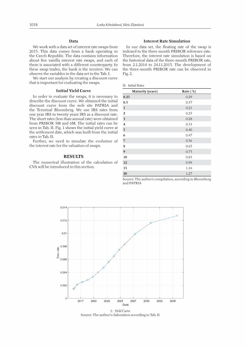
1018 Lenka Křivánková, Silvie Zlatošová

DataWe work with a data set of interest rate swaps from

2015. This data comes from a bank operating in the Czech Republic. The data contains information about five vanilla interest rate swaps, and each of them is associated with a different counterparty. In these swap trades, the bank is the receiver. We can observe the variables in the data set in the Tab. I.

We start our analysis by creating a discount curve that is important for evaluating the swaps.

Initial Yield CurveIn order to evaluate the swaps, it is necessary to

describe the discount curve. We obtained the initial discount curve from the web site PATRIA and the Terminal Bloomberg. We use IRS rates from one year IRS to twenty years IRS as a discount rate. The short rates (less than annual rate) were obtained from PRIBOR 3M and 6M. The initial rates can be seen in Tab. II. Fig. 1 shows the initial yield curve at the settlement date, which was built from the initial rates in Tab. II.

Further, we need to simulate the evolution of the interest rate for the valuation of swaps.

RESULTSThe numerical illustration of the calculation of

CVA will be introduced in this section.

Interest Rate SimulationIn our data set, the floating rate of the swap is

indexed to the three month PRIBOR reference rate. Therefore, the interest rate simulation is based on the historical data of the three-month PRIBOR rate, from 2.1.2014 to 24.11.2015. The development of the three-month PRIBOR rate can be observed in Fig. 2.

II: Initial Rates

Maturity (years) Rate ( %)

0.25 0.29

0.5 0.37

1 0.21

2 0.25

3 0.28

4 0.33

5 0.40

6 0.47

7 0.56

8 0.65

9 0.75

10 0.83

12 0.99

15 1.16

20 1.27

Source: The author’s compilation, according to Bloomberg and PATRIA

1: Yield CurveSource: The author’s elaboration according to Tab. II

Modelling Counterparty Credit Risk in Czech Interest Rate Swaps 1019

We use the Monte Carlo method for the pricing swaps. For more information about this method, see e.g. Hammersley (2013) or Rubinstein and Kroese (2011). One thousand simulations were made. Each of simulations was modelled by the Hull-White model, which is defined by equation (7). We need to estimate parameters α and σ. As described above, the parameters of this model were estimated from three-month PRIBOR. It is α = 0,0208 and σ = 0,015.

The example of yield surfaces obtained in one interest rate simulation is possible to observe in Fig. 3. For each scenario, the swaps are priced at each future simulation date.

In the next text, the probability of default of each client is determined.

2: The Three-month PRIBOR RateSource: The author’s compilation according to Czech National Bank

3: One Possible Scenario of Yield Curve EvolutionSource: The author’s elaboration

1020 Lenka Křivánková, Silvie Zlatošová

Probability of DefaultWe assume that the wait time for a default of

the counterparty is the random variable X with exponential distribution. Then, the cumulative distribution function of this variable can be defined as

( ) ( ) 1 , 0

0, 0

xe xF x P X x

x

λ− − ≥= ≤ = ≤

(11)

where λ > 0 is the parameter of the distribution. The probability of default by the counterparty during one year we denote as PD. Then

( )1 1 PD P X e λ−= ≤ = − (12)

If we use the value of PD from the internal rating model of the bank, which has provided the data, λ could be estimated from (12)

1 PD e λ−= −

( )ln 1 PDλ = − − (13)

Then, we can construct a probability curve for each counterparty. It is possible to observe them in Fig. 4.

Counterparties 3 and 4 have the same rating and counterparties 2 and 5 have the same rating too. Therefore, we can see that their default probability curves are identical.

Computation of CVA Let us consider that the exposure is independent

of default. Then, the total exposure of all contracts can be computed on the bases of equation (4). For estimating of the recovery rate, the bank uses the LGD given by the regulator. According to the European Banking Authority (EBA), the regulatory loss given default is 45 %.

Now we have everything for CVA calculation according to equation (1). The resulting values of CVA for each counterparty can be observed in Tab. III.

DISCUSSIONIn the following section, we turn our attention

to the conflict of the achieved results with the computation of CVA by the bank that provided the data for our calculation. We are drawing a comparison calculation of the CVA that was presented in this paper with the approach that is used in the bank.

4: Default Probability CurvesSource: The author’s elaboration

III: Resulting CVA

Counterparty CVA (in CZK)

1 800,505.82

2 199,337.6

3 276.59

4 783.73

5 78,501.06

Source: The author’s elaboration

Modelling Counterparty Credit Risk in Czech Interest Rate Swaps 1021

The basic principle of the bank’s CVA calculation consists of estimating the expected loss (EL) during a derivative’s live, which is defined as EL = PD ∙ LGD ∙ EAD. For the calculation of the EL of the financial derivative, we divide the remaining time to maturity of the derivative into time frames with a length of one year. The time to maturity is rounded up to a whole year. For each of these frames, the EL of the frame is calculated, then it is discounted and then, finally, all these values are summarised. The result is the CVA. The calculation can be expressed by this relation:

( ) ( ) ( )1

M

i ii

CVA LGD D t EAD t PD i=

= ⋅ ⋅ ⋅∑ (14)

Where M is the number of years to maturity of the financial derivative, and PD(i) is the probability of default during i-th year. A value of LGD is set to 45 % for each counterparty. The bank considers EAD to be constant during a derivative’s live, which is the main difference between their and our approaches. At each point of time, EAD is estimated as the current market value of the financial derivative. The probability of default for each one-year frame of the calculation is computed as follows. For the i-th year:

( ) ( ) 11 iPD i PD PD −= − , (15)

where PD is the average probability of default during one year, which is given by an internal rating of the counterparty. This method of determination of PD is discrete, in contrast to the continuous framework used in this article.

We can observe a comparison of our results of CVA with the CVA used by the bank in Tab. IV. We can see that our results of CVA achieve significantly lower values than the CVA used by the bank.

Another approach in calculating the CVA can be based on a different method of IRS valuation. The approach presented in this paper uses the Hull-White model and Monte Carlo simulations. However, in the literature we can meet with a valuation of the IRS by solving a stochastic differential equation. According to Ševčovič et al. (2011), we can reformulate an interest rate swap agreement such as a coupon bond problem. Using Ito’s lemma, the differential equation for bond price is obtained. This approach, therefore requires an advanced knowledge of the stochastic differential equation. Therefore, our approach is easier and more acceptable for the bank.

The Hull-White model is used in this paper for estimating the interest rate evolution. It is possible to use other models, such as the Vasicek model or Cox-Ingersoll-Ross (CIR) model. However, the Hull-White model is better. Its main advantage is that it can be fitted exactly to the initial term structure of interest rates.

IV: A Comparison of Our Results with the CVA Used by Bank

Counterparty Our results of CVA (in CZK) CVA uses by bank (in CZK)

1 800,505.82 1,646,700.37

2 199,337.6 309,836.82

3 276.59 384.89

4 783.73 1095.12

5 78,501.06 121,149.12

Source: The author’s compilation according to our results and the data set from the cooperating bank

CONCLUSIONThe financial crisis in recent years has shown us how important is to take counterparty credit risk into consideration. It has been presented as a method of counterparty credit risk valuation using credit valuation adjustment. The regulatory requirements for the risk control of the CCR have been summarized. The components of the CVA have been specified. CVA calculation for five various interest rate swaps has been demonstrated. The approach to CVA calculation presented in this article proved to be more profitable than the calculation used in the cooperating bank. If the Bank applied the method of CVA calculation, which is presented in this article, the Bank’s costs of these five IRS would be reduced by 52 %. This means that our paper provides a method to lower capital requirements.

1022 Lenka Křivánková, Silvie Zlatošová

REFERENCESARORA, N., GANDHI, P. and LONGSTAFF, F. A. 2012. Counterparty credit risk and the credit default swap

market. Journal of Financial Economics, 103(2): 280 – 293.BRIGO, D. and MERCURIO, F. 2007. Interest rate models-theory and practice: with smile, inflation and credit.

Berlin: Springer Science & Business Media. CANABARRO, E. and DUFFIE, D. 2003. Measuring and marking counterparty risk. In: Asset/Liability

Management for Financial Institutions, Institutional Investor Books. Euromoney Institutional Investor PLC. [Online]. Available at: http://www.darrellduffie.com/uploads/surveys/duffiecanabarro2004.pdf [Accessed: 2016, November 10].

ČESKÁ NÁRODNÍ BANKA. © 2003 – 2017. Sazby PRIBOR - roční historie. ČNB. [Online]. Available at: https://www.cnb.cz/cs/financni_trhy/penezni_trh/pribor/rok_form.jsp [Accessed: 2015, November 30].

EU. 2013a. Directive 2013/36/EU of the European Parliament and of the Council of 26 June 2013 on access to the activity of credit institutions and the prudential supervision of credit institutions and investment firms, amending Directive 2002/87/EC and repealing Directives 2006/48/EC and 2006/49/EC Text with EEA relevance. Brussels: European Commission.

EU. 2013b. Regulation (EU) No 575/2013 of the European Parliament and of the Council of 26 June 2013 on prudential requirements for credit institutions and investment firms and amending Regulation (EU) No 648/2012 Text with EEA relevance. Brussels: European Commission.

EUROPEAN BANKING AUTHORITY. Article 161. Interactive Single Rulebook. [Online]. Available at: https://www.eba.europa.eu/regulation-and-policy/single-rulebook/interactive-single-rulebook/-/interactive-single-rulebook/article-id/1598. [Accessed: 2016, December 11]

GREGORY, J. 2010. Counterparty credit risk: the new challenge for global financial markets. West Sussex: John Wiley & Sons.

HAMMERSLEY, J. 2013. Monte carlo methods. London: Chapman and Hall.HULL, J. and WHITE, A. 1990. Pricing interest-rate-derivative securities. Review of financial studies,

3(4): 573 – 592.HULL, J. and WHITE, A. 2001. The general hull-white model and supercalibration. Financial Analysts Journal,

57(6): 34 – 43.HULL, J. and WHITE, A. 2012. CVA and wrong-way risk. Financial Analysts Journal, 68(5): 58 – 69.IFSR. 2011. IFRS 13: Fair Value Measurement. [Online]. Available at: http://www.ifrs.org/IFRSs/Pages/IFRS.

aspx [Accessed: 2016, December 11].PATRIA ONLINE. © 1997 – 2017. IRS Sazby historie – CZK. Patria Online. [Online] Available at: https://www.

patria.cz/kurzy/historie/sazby.html. [Accessed: 2015, October 30]PYKHTIN, M. and ROSEN, D. 2010. Pricing counterparty risk at the trade level and CVA allocations. Journal

of Credit Risk, 6(4): 3 – 38.PYKHTIN, M. and ZHU, S. H. 2007. A guide to modeling counterparty credit risk. GARP Risk Review, 37: 16 – 22.RUBINSTEIN, R. Y. and KROESE, D. P. 2011. Simulation and the Monte Carlo method. Hoboken: John

Wiley & Sons.ŠEVCOVIC, D., STEHLIKOVÁ, B. and MIKULA, K. 2011 Analytical and numerical methods for pricing financial

derivatives. New York: Nova Science Pub. Inc.

Contact information

Lenka Křivánková: 142474@mail.muni.czSilvie Zlatošová: 175424@mail.muni.cz