Embed Size (px)
Citation preview

Modelling and monitoring
thermal response of the
ground in borehole fields
Patricia Monzó
Doctoral Thesis, 2018
KTH Royal Institute of Technology
School of Industrial Engineering and Management
Applied Thermodynamics and Refrigeration Division
SE-100 44 Stockholm, Sweden

TRITA-ITM-AVL 2018:1
ISSN 1102-0245
ISRN KTH/REFR/18/01-SE
ISBN 978-91-7729-667-6
Dissertation presented at Royal Institute of Technology, KTH, to be publicly examined in
Lecture Hall D2, Lindstedtsvägen 5, Plan 3, Stockholm, Friday, 23 February 2018 at 10:00
for the degree of Doctor of Philosophy. The examination will be conducted in English.
Patricia Monzó, February 2018

To my dad, Antonio J. Monzó

i
Abstract
This Ph.D. dissertation aimed at developing tools for the evaluation of
ground response in borehole fields connected in parallel through modelling and
monitoring studies.
A total heat flow and a uniform borehole wall temperature condition equal
in all boreholes have often been accepted when mathematically modelling the
response of vertical ground heat exchangers connected in parallel. The first
objective of this thesis was the development of a numerical model in which the
ground controls the temperature response at the borehole wall, instead of imposing
heat flow or temperature conditions at this interface. The unavoidable fluid-to-
borehole wall thermal resistance and the variation of the heat flux distribution
along the borehole depth violates the assumption of uniform temperature at the
borehole wall. This aspect, which is often disregarded, was taken into account in
this model. The results obtained from the numerical simulations are believed to
come closer to reality and can be used as a reference for other approaches.
When bore field sizing, the worst ground load conditions are usually
assumed to occur after several years of operation, but these may occur during the
first year of operation. The second objective of this work was the development of
a general sizing methodology that calculates the total required bore field length for
each arbitrary month during the lifetime of the installations. The methodology was
also used to investigate to what extent the borehole spacing can be reduced without
increasing the total required bore field length when the ground load condition is
thermally quasibalanced.
The ground source heat pump community still lacks detailed and accurately
measured long-term data for validation of modelling tools. In order to partially
contribute to filling this gap, the last part of this Ph.D. study focused on state of
the art monitoring activities. The main goal of this part is to provide a
comprehensive description of the ground thermal loads and response
measurements at a large bore field, that is being monitored from the beginning of
its operation. Unique data sets, showing the thermal loads and ground thermal
response during extraction and injection, along with measurement error analyses
are reported in the thesis.
Keywords: ground temperature response, borehole heat exchanger,
modelling, monitoring, sizing


iii
Sammanfattning
I denna doktorsavhandling presenteras nya verktyg för utvärdering av
berggrundens respons i geotermiska borrhålslager där borrhålen är kopplade
parallellt. Avhandlingen beskriver både modellering och fältstudier.
Ett givet totalt värmeflöde och likformiga väggtemperaturer i alla borrhålen
har ofta varit accepterade randvillkor vid matematisk modellering av den termiska
responsen av parallellkopplade borrhålsvärmeväxlare i grupper av vertikala
borrhål. Det första målet i arbetet med denna avhandling var att utveckla en
numerisk modell i vilken berggrunden tillåts bestämma temperaturresponsen vid
borrhålsväggen, istället för att som randvillkor ange ett visst värmeflöde eller en
viss temperatur. Det ofrånkomliga värmemotståndet mellan flödet i
slangen/värmeväxlaren och bergväggen och variationen i värmeflöde längs
borrhålet innebär att dessa förenklade antaganden inte stämmer. Denna aspekt,
som ofta förbisetts, har inkluderats i den här presenterade modellen. Resultaten
som erhållits med denna numeriska modell kan förväntas vara närmare
verkligheten än tidigare modeller och kan användas som referens för andra
beräkningar.
Vid dimensionering av borrhålslager antas vanligen de värsta
berggrundstemperaturerna inträffa efter flera års drift, men i avhandlingen visas
att de värsta förhållandena kan uppstå under det första driftåret. Det andra målet
med arbetet var att utveckla en generell dimensioneringsmetodik som kan
användas för att beräkna den totala nödvändiga borrhålslängden för varje månad
under installationens hela livslängd. Metodiken användes också för att undersöka
i vilken mån borrhålsavståndet kan minskas utan att den totala borrhålslängden
behöver ökas, under förutsättningen att borrhålslagret är ungefär balanserat.
Forskarsamhället saknar fortfarande detaljerade och noggrant uppmätta
långtidsdata som kan användas för att validera olika modelleringsverktyg. I avsikt
att i någon mån bidra till att fylla detta tomrum, innehåller den sista delen av
avhandlingen beskrivningar av god teknik för utvärdering av
borrhålslager. Huvudmålet för denna del av avhandlingen är att ge en utförlig
beskrivning av värmelasterna och responsmätningarna i ett stort borrhålslager som
studerats sedan det först togs i bruk. Unika data rörande termiska laster och
berggrundens termiska respons under värmeuttag och värmelagring, samt
felanalys, presenteras i denna avhandling.
Nyckelord: bergtemperaturrespons, borrhålsvärmeväxlare, modellering,
övervakning, dimensionering.


v
Acknowledgements
It is said that the best part of a journey is not at the destination, but at the
journey itself. Indeed, that is how I understand it as well! The best part of this work
has been the journey, I don’t have any doubts about it: people I met, friends I made,
all the learning about boreholes and energy systems, field work activities, the
Ph.D. stay in Montréal, research collaboration with other universities,
challenges… and mistakes, deadlines, stressful moments, conferences,
nervousness before presentations, post-travelling conferences, meeting and social
meetings, learning about Swedish culture, and any other culture in the world due
to the great family we are at KTH. In the end, all the moments we shared. These
all made my journey great. Thanks a lot!
Of course, this journey wouldn’t have been possible without the support I
received from numerous people along this journey.
Firstly, I would like to deeply acknowledge Prof. Björn Palm for giving me
the opportunity to conduct my Ph.D. study within his research group at the
Division of Applied Thermodynamics in the Energy Department at KTH. The first
stage of this Ph.D. work was part of a research project in the Material Science
Department at KTH. Thanks to Prof. Folke Björk for this opportunity.
Thanks also to Prof. Björn Palm for being the main supervisor of my work,
providing me with your guidance, support during all of this work and for giving
me the opportunity to engage in interesting projects and collaborations with other
research groups.
There are two very special people to whom I am deeply grateful, José
Acuña and Palne Mogensen. This achievement is also yours!
José Acuña, thanks for your support and guidance during all this time.
Thousand thanks for your patience. Finally this is happening! Keep on being so
enthusiastic and motivated by your work. Dreams come true for believers!
Palne Mogensen, a person who I really look up to. Thanks for being a
research advisor of my Ph.D. study, sharing with me your knowledge about ground
heat exhangers and your valuable discussions. Many thanks for the idea of the
highly conductive material for modelling the response of ground in bore fields!

vi
I would also like to express my deep gratitude to Prof. Michel Bernier.
Thank you for hosting me as a visitor researcher at Polytechnique Montréal.
Thanks for giving me the opportunity to take the course and to work with you in a
research project that became part of this work. Thanks also to the research group
at EPM, especially to Massimo, Bruno and Amir, for all the discussions and good
times during my stay.
I would also like to acknowledge the Swedish Research Council FORMAS,
the seventh research framework programme “advanced ground source heat pump
systems for heating and cooling in Mediterranean cliamtes” Ground-Med
TREN/FP7EN/218895 the Swedish Energy Agency and the industrial sponsors:
Akademiska Hus, Hesselmannska stiftelsen, Skanska, Stures brunnsborningar,
Tyréns for co-financing this work.
Thanks to Jan-Erik Nowacki for your research curiosity and valuable
perspective which turned up in one of the research topics of this work. Thanks to
Prof. Marco Fossa, Prof. José Miguel Corberán and his research group,
practicularly to Carla, Felix, Javi y Antonio, for giving me he opportunity to
collaborate with them in interesting research projects. Thanks to Anjan,
Alexandro, Mauro, Marc, Jens, Jesús.
Thanks to the KTH family for your support and all the great moments.
Thanks to Mazyar for being “the officemate”. Special thanks to David, Jonas,
Nelson, Monika, Pavel, Enrique, Oxana, Peter, Hatef, Joakim, Per, Jaime, Erik,
Benny, Luis and Nordin. Let me know if you want me to prepare popcorns! Also
thanks to Antonio, Monika, Mauri, Tobias, Paul, Eunice, Sara, Saman, Maria,
Rafa, Nenad, Lukas, Johan, Björn, Jorge and Monica from the other side of the
kitchen.
Thanks to the KTH geo-group, Alberto, Willem, Mohammad, Davide,
Monika and Letizia, for your discussions, an insatiable research curiosity and all
good times. Thanks to Alberto for his help with Julia and Frescati. Special thanks
to Willem, Mohammand and Enrique for their willingness to help me in Frescati.
I believe that all these good opportunities with so very nice people were not
a coincidence. These were sent by my angel. I have an angel, my father, to whom
I dedicate all this work. Thanks for taking care of me at every single moment!
Special memory for my grandparents, Carmen y Antonio, and Benedicta and
Candido, and my uncle, Juan.
I deeply thank to my family, especially to cousin Andrés, and friends in
Spain for their support no matter what it is, no matter distance and no matter time.

vii
I am also grateful to all the friends I made during this journey, especially to Manu,
Amparo, Laura, Edu, Guillem, Flo, Isa, Teresa, Yenni y Ale, Anne, Bernardo, Bea,
Vicky, Mamem, Pedro and Fran.
Y por supuesto, a ti también, Mamá, todo un ejemplo a seguir. Muchísimas
gracias por apoyarme en todo lo que hago y por recordarme cada día que no me
olvide de sonríe. Gracia a ti y al papá, por la educación y lo valores que nos distéis
a mi y a mi hermano. No hubiésemos podido llegar hasta aquí sin vosotros. Gracias
por hacer de mi hermano mi mejor amigo. Juan, mil gracias por apoyarme en esta
aventura y en todo lo que se me ocurra hacer y de manera incodicional. Gracias,
por los dibujos de la tesis. María, muchas gracias también a ti por tu apoyo y por
todos los buenos momentos. Y por último, y aunque no menos importante, mil
gracias a Jesús, por su apoyo, por su infinita paciencia y por hacerme reir mucho.
Contigo todo ha sido mucho más fácil. ¡Muchas gracias mi querida familia!
¡Estoy también es vuestro! ¡Os quiero!
Thanks to everyone for making this achivement to happen!


ix
Contents 1. INTRODUCTION ........................................................................................................................... 1
1.1 Overall context ...................................................................................................................... 1
1.1.1 Current situation and R&D projects in Europe ............................................................ 2
1.2.1 Current situation and R&D plans in Sweden ............................................................... 3
1.2.2 Context of this doctoral work ...................................................................................... 5
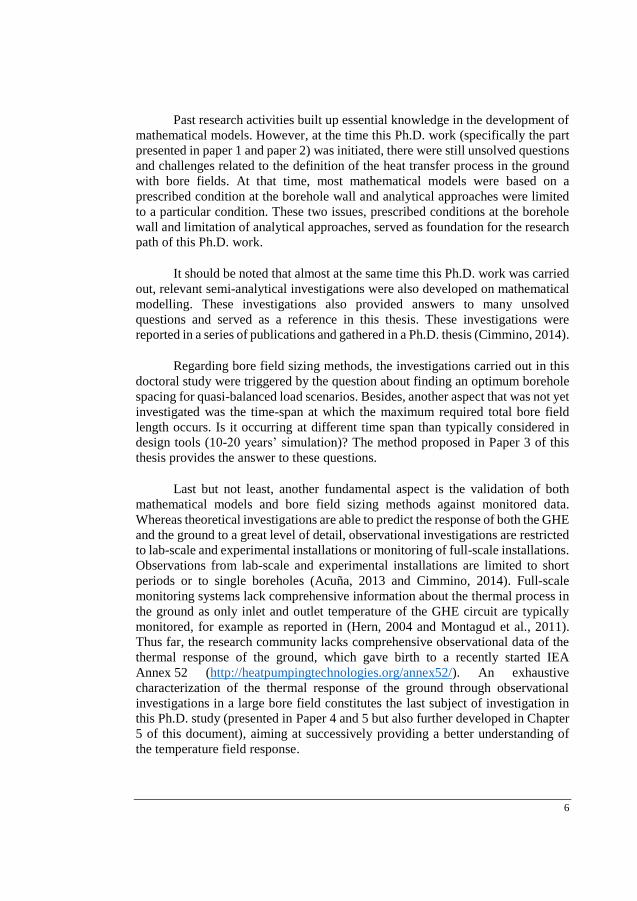
1.2 Research Objective ................................................................................................................ 7
1.3 Structure of the thesis ............................................................................................................ 7
2 BACKGROUND & EARLIER WORK ......................................................................................... 11 2.1 Vertical ground heat exchangers in parallel connection ....................................................... 11
2.1.1 System description and system operation .................................................................. 11
2.1.2 Heat transfer inside the borehole ............................................................................... 14
2.1.3 Heat transfer process in the ground ........................................................................... 15
2.1.4 Solutions to the heat transfer process in the ground .................................................. 19
2.2 Boundary conditions in mathematical modelling of GHEs connected in parallel ................ 21
2.2.1 Constant heat flux at the borehole wall in all boreholes ............................................ 21
2.2.2 Equal average borehole wall temperature in all boreholes......................................... 22
2.2.3 Uniform borehole wall temperature in all boreholes ................................................. 22
2.2.4 Same inlet fluid temperature in all boreholes ........................................................... 22
2.2.5 Discussion about boundary conditions and its relation to this work .......................... 23
2.3 Simulation of ground temperature response and bore field sizing methods ......................... 28
2.3.1 The g-function ........................................................................................................... 29
2.3.2 The ASHRAE method ............................................................................................... 32
2.4 Monitoring of borehole field response ................................................................................. 33
3 MODELLING THE THERMAL RESPONSE OF THE GROUND IN BOREHOLE
FIELDS ...................................................................................................................................... 37 3.1 Specific objective ................................................................................................................ 37
3.2 Method ................................................................................................................................ 37
3.3 The highly conductive material model and its enhanced version ......................................... 38
3.3.1 Concept of the highly conductive material ................................................................ 38
3.3.2 Computing geometry and mesh ................................................................................. 42
3.4 Results ................................................................................................................................. 43
3.4.1 TRF generation ......................................................................................................... 44
3.4.2 Illustration of fluid temperature predictions for measured load. Comparison with
measured data. ........................................................................................................................ 46
3.5 Conclusions ......................................................................................................................... 51
4 BORE FIELD SIZING: INFLUENCE OF DESIGN PARAMETERS ........................................... 53 4.1 Specific objective ................................................................................................................ 53
4.2 Method ................................................................................................................................ 53
4.3 Development of a general bore field sizing methodology .................................................... 54
4.3.1 Development of the formulation for the total bore field length calculation at the end
of each month ......................................................................................................................... 54

x
4.3.2 Methodology for calculation of the total bore field length ........................................ 58
4.4 Application of the methodology .......................................................................................... 60
4.4.1 Calculation of the required total bore field length at the end of each month during the
first year of operation .............................................................................................................. 60
4.4.2 Optimum borehole spacing ....................................................................................... 61
4.5 Conclusions ......................................................................................................................... 63
5. MONITORING THE THERMAL RESPONSE OF A BOREHOLE FIELD ................................. 65
5.1 Specific objective ................................................................................................................ 65
5.2 Method ................................................................................................................................ 65
5.3 Implementation of the monitoring set-up ............................................................................. 66
5.4 Description: installation, bore field and monitoring system ................................................. 67
5.4.1 Description of the installation ................................................................................... 67
5.4.2 Ground load condition ............................................................................................... 68
5.4.3 Description of the bore field ...................................................................................... 68
5.4.4 Monitoring system .................................................................................................... 69
5.5 Presentation of the bore field measurements. Measurement error analysis .......................... 73
5.5.1 Commissioning and status of the monitoring system ................................................ 73
5.5.2 Presentation of the power meter measurements in the monitored manifolds and
boreholes. Analysis of the measurement errors. ...................................................................... 74
5.5.3 Presentation of the DTS measurements in the monitored boreholes. Assessment of the
signal losses in the DTS measurements. ................................................................................. 91
5.6 Bore field measurements during the first year of operation ................................................. 96
5.7 Conclusions ......................................................................................................................... 97
6. CONCLUSIONS ............................................................................................................................ 99
6.1. Discussion and Future Work ............................................................................................... 100
REFERENCES ................................................................................................................................ 103
APPENDIX A ................................................................................................................................. 109
A.1. Arrangements of the power meters within the piping circuit in the measurement wells ..... 109
A.2. Comparison of the inlet fluid temperatures in each of the monitored manifold against its
relative monitored borehole........................................................................................................ 113
A.2.1. Comparison of the inlet fluid temperatures in each of the monitored manifold against its
relative monitored borehole for a period of 5 days in February,2017 (minutely measurements) 113
A.2.2. Comparison of the inlet fluid temperatures in each of the monitored manifold against its
relative monitored borehole: September 8, 2016 - July 7, 2017 (minutely measurements)......... 115
APPENDIX B.................................................................................................................................. 119
B.1. DTS measurements – assessment of signal losses in terms of temperature ......................... 119
Temperature measurements of the reference sections in the bath 1 at a zero-degree Celsius
constant temperature ............................................................................................................. 119
Temperature measurements of the reference sections in bath 2 at a zero-degree Celsius
constant temperature ............................................................................................................. 120
Temperature measurements of the reference sections in bath 3 at a zero-degree Celsius
constant temperature and at an outdoor temperature. ............................................................ 121
B.2. Fiber cable set-up and reference section ............................................................................. 122
xi
Index of Figures
Figure 1 Outline and context of the structure of the thesis. .................................................................. 7
Figure 2 Components of a GHE with a single U-pipe arrangement (left-side) and description of
geometrical parameters in a bore field with vertical boreholes (right side). ....................................... 13
Figure 3 Diagram of the thermal process in the ground with uniform fluid, temperature condition. .. 26
Figure 4 Connection of the boreholes to HCM bar. One-eigth geometry of a 4×4 bore field
configuration. ..................................................................................................................................... 39
Figure 5 Hemispherical bottom element of the borehole in 3D space dimension. ............................. 41
Figure 6 Normalized (a) heat flux and (b) temperature along borehole length for a 2×3 bore field
(geometrical aspect ratios as shown in Figure 11, (k=3.5 W/(m-K); Rb= 0.1(m-K)/W ) at ln(t/ts)=0.1
(25 years for H=100 and α=1.5810-6 m2/s) resulting from the HCM and the EHCM models. ........... 42
Figure 7 Computing domain for a 4×4 bore field and mesh elements in the adjacent region to the
boreholes. .......................................................................................................................................... 44
Figure 8 TRFs for a 4×4 bore field for a given geometrical aspect ratios (k=3.5 W/(m-K);
Rb= 0.1 (m- K)/W in the EHCM model). .......................................................................................... 46
Figure 9 Daily fluid temperature predictions using FEM models and comparison with measured data
for ‘Facility 1’. .................................................................................................................................. 49
Figure 10 Daily fluid temperature predictions using FEM models and comparison with measured data
for ‘Facility 2. .................................................................................................................................... 50
Figure 11 Illustration of the calculations of the ground load and effective ground thermal resistance for
the preceding month term in Equation 11 for the case i=3. ................................................................ 55
Figure 12 Illustration of the calculations of the ground load and effective ground thermal resistance for
the current month term in Equation 11 for the case i=3. .................................................................... 56
Figure 13 Illustration of the calculations of the ground load and effective ground thermal resistance for
the peak load term in Equation 11 for the case i=3. ........................................................................... 56
Figure 14 Illustration of the calculations of the ground load for the temperature penalty in Equation 11
for the case i=3. ................................................................................................................................. 57
Figure 15 Flowchart containing the steps of the iterative process to calculate L in Equation 11
(presented in Paper 3). ....................................................................................................................... 59
Figure 16 Calculation of L for different values of B during the first year of operation and two different
starting dates: January 1 and July1. ................................................................................................... 62
Figure 17 Calculation of L for different values of B during the tenth year of operation and two different
starting dates: January 1 and July 1. .................................................................................................. 62
Figure 18 Plan view of the monitored bore field in the BTES installation ......................................... 69
Figure 19 Measuring procedure of power measurements in the monitored manifold and boreholes along
with some pictures of bore field components during their installation. .............................................. 70
Figure 20(a) Sketch of the fiber connection in the boreholes and to the DTS instrument in channel 3
and (b) temperature measurements along the entire fiber path at a certain interval during calibration
activities. ........................................................................................................................................... 72
Figure 21 (a) Inlet and outlet temperatures, (b) volume flow rate measurements measured in the
monitored manifolds during five days in February 2017. .................................................................. 74
Figure 22 (a) Inlet and outlet temperatures, (b) volume flow rate in the monitored boreholes during five
days in February 2017. ...................................................................................................................... 75
Figure 23 Inlet and outlet temperatures in the monitored manifolds during one day in February 2017
(minutely values). .............................................................................................................................. 77
Figure 24 Inlet and outlet temperatures in monitored boreholes during one day in February 2017
(minutely values). .............................................................................................................................. 77
xii
Figure 25 Minutely measurements of the inlet and outlet temperatures in BH12 and MF2 during a
period of five days in February 2017. ................................................................................................ 78
Figure 26 Existing location of power meters (volume flow rate meter and temperature sensor at the
inlet and return pipes) in the measurement well of MF2 and BH12. ................................................. 79
Figure 27 Inlet temperature of BH12 vs corresponding manifold inlet temperature, MF2, for the period
between September 8, 2016 and July 11, 2017 (minutely measurements). ........................................ 80
Figure 28 Temperature measurements during calibration of the inlet temperature sensor in MF2. .... 82
Figure 29 Temperature measurements during calibration of the inlet temperature sensor in MF3. .... 82
Figure 30 A photo taken during the test performed to measure the resistance of the temperature sensor
at the inlet pipe of MF2. .................................................................................................................... 83
Figure 31 Temperature measurements (minutely values) of the sensors located at the supply and return
pipes of the monitored manifolds and boreholes on April 7, 2016 ..................................................... 85
Figure 32 Monitored raw data of the power meter in BH12 during the period between September 8,
2016 and January 23, 2018 ................................................................................................................ 90
Figure 33 Temperature measurements along the borehole depth at three different periods in BH6 and
BH12. ................................................................................................................................................ 91
Figure 34 Channel 3: fiber set-up and summary of the signal losses in terms of temperature at the
reference sections .............................................................................................................................. 94
Figure 35 Temperature measurements along the length of the monitored boreholes BH6, BH12 at three
different given periods along with the corresponding measured heat flow (W/m) at the three given
times and for the whole monitored period. ........................................................................................ 96
Figure 36 Measurement well of MF1 and BH6 ............................................................................... 109
Figure 37 Measurement well of MF2 and BH12 ............................................................................. 109
Figure 38 Measurement well of MF3, BH16,BH18 and BH21 ........................................................ 110
Figure 39 Measurement well of MF4, BH24 and BH38 .................................................................. 110
Figure 40 Measurement well of MF5 and BH45 ............................................................................. 111
Figure 41 Measurement well of MF7 and BH62 ............................................................................. 111
Figure 42 Measurement well of MF12 and BH105 .......................................................................... 112
Figure 43 Minutely measurements of the inlet and outlet temperatures in BH16, BH18,BH21 and MF3
during a period of five days in February 2017. ................................................................................ 113
Figure 44 Minutely measurements of the inlet and outlet temperatures in BH24 and MF4 during a
period of five days in February 2017. .............................................................................................. 113
Figure 45 Minutely measurements of the inlet and outlet temperatures in BH45 and MF5 during a
period of five days in February 2017. .............................................................................................. 114
Figure 46 Minutely measurements of the inlet and outlet temperatures in BH62 and MF7 during a
period of five days in February 2017. .............................................................................................. 114
Figure 47 Minutely measurements of the inlet and outlet temperatures in BH105 and MF12 during a
period of five days in February 2017. .............................................................................................. 114
Figure 48 Comparison of the inlet fluid temperature of MF3 and its relative monitored BH16 ....... 115
Figure 49 Comparison of the inlet fluid temperature of MF3 and its relative monitored BH18 ....... 115
Figure 50 Comparison of the inlet fluid temperature of MF3 and its relative monitored BH21 ....... 116
Figure 51 Comparison of the inlet fluid temperature of MF4 and its relative monitored BH24 ....... 116
Figure 52 Comparison of the inlet fluid temperature of MF5 and its relative monitored BH45 ....... 117
Figure 53 Comparison of the inlet fluid temperature of MF7 and its relative monitored BH62 ....... 117
Figure 54 Comparison of the inlet fluid temperature of MF12 and its relative monitored BH105 ... 118
Figure 55 Temperature measurements of the reference sections of channel 3 in bath 1. .................. 119
Figure 56 Temperature measurements of the reference sections of channel 3 in bath 2. .................. 120
Figure 57 Temperature measurements of the reference sections of channel 3 in bath 3 ................... 121
Figure 58 Fiber set-up and reference sections in channel 1 .............................................................. 122

xiii
Figure 59 Fiber set-up and reference section in channel 2 ............................................................... 123
Figure 60 Fiber set-up and reference section in channel 4. .............................................................. 124
Index of Tables
Table 1 Summary of performance specifications of the monitoring equipments with regards to
instrument settings at the actual monitoring site. ................................................................. 66
Table 2 Summary of the monitoring equipment within the bore field: location and actual status of the
power and of the DTS equipments. (September 2017). ........................................................ 73
Table 3 Summary of the inlet fluid temperature comparison: manifold against relative borehole. .... 81
Table 4 Analysis of temperature measurements in the monitored boreholes during April 7, 2017 . .. 84
Table 5 Analysis of the inlet and outlet temperature measurements in the boreholes against the
reference temperature Tref,BH.. .............................................................................................. 87
Table 6 Analysis of temperature measurements in the monitored manifolds during the selected periods
in April 7, 2017 . .................................................................................................................. 87
Table 7 Analysis of the inlet and outlet temperature measurements in the manifolds against the
reference temperature Tref, BH ................................................................................................ 88
Table 8 Analysis of the volume flow measurements in the monitored manifolds and boreholes during
February 7, 2017. ................................................................................................................. 89
Table 9 Summary of the analysis of the signal losses at the reference sections in channel 3. ............ 95


xv
NOMENCLATURE
Latin Symbols
B Borehole spacing m
cp heat capacity J/(Kg-K)
D Inactive upper part of the borehole m
Fo Fourier number, with rb as the characteristic length -
FoH Fourier number, with H as the characteristic length -
G Non-dimensional temperature response factor based on
CHS solution -
g Gravitational constant m/s2
g Non-dimensional temperature response factor based on a
uniform borehole wall temperature boundary condition
g1 g-Function for the single borehole at the time at which Tp
is evaluated (typically 10 years) -
g1,i g-Function for the single borehole for the month i with
i=1 to 12 -
gn g-Function for the selected multiple bore field at the time
at which Tp is evaluated (typically 10 years) -
gn,i g-Function for the selected multiple bore field for the
month i with i=1 to 12 -
H Total active borehole length m
k Thermal conductivity of the ground W/(m-K)
kTRL Thermal conductivity of the thermal resistive layer W/(m-K)
lf,loop Head loss (the equivalent height of a column of the
working fluid) m
L Total required bore field length m
Li Total required bore field length for the month i with i=1
to 12 m
nb Number of boreholes -
∆P Pressure loss Pa
Pf Pumping power W
Q Total heat flow W
q Heat flow per unit length W/m
q′ Normalized heat flow per borehole -
qm Monthly ground load evaluated when qh occurs W
qcm,i Average ground load for the month i with i=1 to 12 W
qh Hourly peak load for heating and cooling, separately W
qh,i Hourly peak load for the month i with i=1 to 12 W
qpm,i Average ground load preceding the month i with i=1 to
12 W
qy Yearly average ground load W
Rb GHE local thermal resistance (m-K)/W
Rb* GHE effective thermal resistance (m-K)/W
xvi
Rpm.i Effective ground thermal resistance relative to qpm,i (m-K)/W
Rcm Effective ground thermal resistance relative to qcm,i (m-K)/W
Rh Effective ground thermal resistance relative to qh,i (m-K)/W
R10y Effective ground thermal resistance relative to qy (m-K)/W
R1m Effective ground thermal resistance relative to qm (m-K)/W
R6h Effective ground thermal resistance relative to qh (m-K)/W
rb Borehole radius m
Re Reynolds number -
t Time s
tS H2 9α⁄ Characteristic time s
T Temperature ºC
Tbw Average borehole wall temperature ºC
Tf Simple mean fluid temperature ºC
Tf,z Mean fluid temperature at a given borehole depth z ºC
Tfiber cable Temperature of the fiber cable (Table 9) ºC
Tg Undisturbed ground temperature
Tin,BH Inlet temperature of the borehole ºC
Tout,BH Outlet temperature of the borehole ºC
Tin,MF Inlet temperature of the manifold ºC
Tout,MF Outlet temperature of the manifold ºC
Tref,BH Average temperature of BH6, BH12, BH18, BH24,
BH45, BH105 at any given time ºC
Tref. sensor Temperature of the reference sensor (Table 9)
Tp Temperature penalty ºC
�� Volume flow rate l/s
��𝐵𝐻 Volume flow rate in the borehole l/s
��𝑀𝐹 Volume flow rate in the manifold l/s
Subscript
ds Downstream (forward path of the laser in the fiber cable)
in Inlet fluid temperature
inner Borehole located at the center of a 3×1 bore field configuration (Figure 3)
out Outlet fluid temperature
outer Borehole located at the outward of a 3×1 bore field configuration (Figure 3)
s Soil
us Upstream (backward path of the laser in the fiber cable)
Superscript
Average

xvii
Greek Symbols
𝛼 Thermal diffusivity m2/s
δTRL Thickness of the thermally resistive layer m
𝜌 Density kg/m3
ν Velocity of the fluid m/s
Standar deviation
ABBREVIATIONS
BH Borehole
C Fiber cable connection (Table 9)
CHS Cylindrical heat source
EED Earth energy designer design tool
EHCM Enhanced highly conductive material
FDM Finite difference method
FEM Finite element method
FLS Finite line source
GCHP Ground-coupled heat pump
GHE Ground heat exchanger
GLHEPRO Ground loop heat exchanger professional
g-function non-dimensional temperature response factor (Equation 5)
HCM Highly conductive material
JB Junction box (splice of the fiber)
MAE Mean absolute error
MBE Mean bias error
RHC Renewable heating & cooling
RMSE Root mean square error
RS Reference section (Table 9)
S Splice (Table 9)
S-EL End-loop splice (Table 9)
SBM Superposition borehole model
TRF Temperature response function (see discussion in Chapter 3.4.1)
TRL Thermally resistive layer

1
1. INTRODUCTION
This introductory chapter addresses the overall context and the unresolved challenges
of the research topic treated in this dissertation. Next, the objectives of this dissertation are
stated, and the methodology is described. The structure of the thesis is presented at the end
of this chapter.
1.1 Overall context
The scope of this dissertation is on ground coupling technologies that
employ buried closed-loop heat exchangers in the ground to extract and/or inject
heat to either provide space heating and/or cooling or to create an underground
heat/cold storage with a similar end-use application (space heating or cooling).
The assistance of a heat pump is normally required in these systems.
The ground temperature, except in the upper few meters, is relatively
stable, higher than the outdoor temperature during winter, and opposite during
summer,which makes the ground an attractive heat source or a sink for heat pump
systems. Since the temperature of the ground changes while extracting or injecting
heat, coupling technologies require design rules and simulation tools to predict
ground temperature response to the intended heat load.
A ground heat exchanger (GHE) is a buried pipe embedded within a drilled
hole in the ground, a.k.a. borehole. Thus, the heat is exchanged with the
surrounding ground as a secondary fluid, at a temperature different than the
surrounding ground, circulates downwards and upwards in the pipe arrangement
inside the borehole. The temperature difference between the secondary fluid and
the surrounding ground induces heat transfer. The GHEs are commonly single U-
pipe and double U-pipe types. The overall group of heat exchangers embedded in
the boreholes constitute the bore field.
In ground-coupled heat pump (GCHP) systems, the GHEs circuit is
coupled to the heat pump (except for free cooling mode) so that the heat pump
moves the heat from the low-temperature source (ground - outdoor circuit) to the
high-temperature sink (building - indoor circuit) in heating mode and vice versa
for cooling purposes. Nowadays, these systems are recognized as one of the most
ecofriendly alternatives for space heating and cooling in buildings due to their high
efficiency and low environmental impact, contributing effectively to the
mitigation of CO2 emissions.
2
With respect to thermal storage systems, a closed-loop of a large number
of densely packed GHEs are employed to create actively and intentionally a
storage of sensible heat in the underground. This technology is known as borehole
thermal energy storage (BTES). In space heating and cooling applications, BTES
systems have the potential to improve the efficiency of the systems and to integrate
several energy systems within the building envelope. For instance, by storing
thermal energy from a solar source and/or waste energy from chillers, space/water
heating demand is satisfied when the availability of solar energy is limited. Some
BTES installations do not necessarily require the assistance of a heat pump.
Several examples that are currently in operation, cited in (Gehlin and Andersson,
2016), illustrate the versatility of BTES systems.
1.1.1 Current situation and R&D projects in Europe
Nowadays, figures of installed units in Sweden, Germany or Switzerland
reflect the fast market growth of GCHP systems in northwestern Europe during
the last decades, for mainly space heating applications. Several factors, such as
climatic conditions, geological conditions, progress of the drilling technique,
awareness of heat pump performance for space heating applications, interest of
buildings’ stakeholders in GCHP systems, reasonable installation cost, low
running costs, policies and incentives fostered GCHP technology in cold climate
countries.
On the contrary, in southern European countries, heating is still mainly
provided by fossil-based methods and cooling is mostly supplied from electricity
systems with large carbon footprint (Tanaka and others, 2011). A recently ended
European research project that partly financed this doctoral work, GROUND-
MED (Ground-Med 2009-2014), focused on confirming the viability of ground
coupled heat pump technology in 8 demonstration sites located in Mediterranean
climate for space heating and cooling. A fast growth of emerging GCHP markets
in Italy, Spain, the United Kingdom, Hungary, Romania, Poland, and the Baltic
states is expected over the upcoming years as reported in a roadmap report of the
renewable heating & cooling (RHC) Platform (Aposteanu et al., 2014). High
prices (and high taxes) on fossil fuels may also favor the heat pump market growth.
As for BTES systems, a number of these can also be found in Europe. Early
installations were compiled in (Hellström, 1991). Most of the early installations
were installed in Sweden and the borehole depths ranged between 6 - 110 m. As
technologies in drilling and in heat pump performance progress, deeper boreholes
(>150 m) are being drilled in this kind of system. More recent BTES plants were
reported in (Gehlin, 2016).
3
In this context, in which technology of ground coupling systems is quite
mature and is commercially available, both GCHP and BTES systems are thought
to play an important role during the upcoming years for space heating and cooling
in the building sector as reported in the “Technology Roadmap: Energy-efficient
Buildings: Heating and Cooling Equipment” elaborated by the International
Energy Agency, (Tanaka and others, 2011).
In line with the future plans to move forward to sustainable energy
scenarios, the European Union is currently supporting a large energy research and
innovation program - Horizon 2020. A quote of the research and innovation
program in Horizon 2020 is related to ground coupling technologies in the call
(“HORIZON 2020 - Work Program 2016 - 2017. ‘Secure, Clean and Efficient
Energy,’” 2017).
Besides, the RHC - platform (Aposteanu et al., 2014) also defines an
outline for R&D activities in Europe on shallow geothermal systems with the main
focus on GCHP systems. This outline is consonant with the IEA roadmap for
future energy scenarios and the schedule in Horizon 2020 program. The outline
of the R&D activities has its main target on the reduction of installation cost and
the increasing of the heat exchange efficiency in order to consolidate GCHP
systems in developed and developing markets. RHC - platform suggests R&D
efforts to be targeted for the development of improved and innovative drilling
techniques to reduce its cost and its impact in the surrounding and to control
borehole deviation. In the RHC – platform’s outline it is suggested that the R&D
activities should aim at improving heat transfer efficiency with the surrounding
ground via optimization of borehole components, design and heat pump
components. Specific R&D plans are not found for BTES systems in (Aposteanu
et al., 2014).
With regard to matters of increase and optimization of system efficiency
and reduction of cost, BTES systems may share similar challenges as the ones
specified for GCHP. Moreover, BTES systems have the potential to create low or
medium temperature heat storage applications which have a thermodynamical
advantage for integration of systems. This subject may be of a great interest for
R&D plans in Europe and with existing project in northwestern Europe.
1.2.1 Current situation and R&D plans in Sweden
Expertise and figures of installed capacity of ground coupling technologies
yield Sweden as a leading country in this field as reported in (Erlström et al., 2016)
and in the European heat pump market and statistic report (Nowak and Westring,
2016).

4
The oil crisis in the 70’s prompted policies and economic incentives
towards oil-independent energy systems based on renewable sources. In that
context, the utilization of shallow geothermal resources (low-enthalpy) in
combination with heat pump technology attracted a lot of interest. Thus, the GCHP
systems with a vast majority of vertical ground loops started to play a major role
in replacing fossil fuel for space heating in buildings, mainly in small residential
buildings during the late 70’s and 80’s and with a rapid growth in the 90’s.
At the same time, extensive research work was developed in this field. One
of the first activities to find methods to assess the properties of the ground was
carried out by (Mogensen, 1983), who proposed and tested a method to evaluate
the borehole thermal resistance while finding thermal properties of the ground in
a thermal response test. (Eskilson, 1986 and Claesson and Eskilson, 1987)
developed a methodology to evaluate the long-term response of multiple bore
fields, (Hellström, 1991) studied local and global thermal processes in GHEs and
surrounding ground.
Past and continuous present efforts have led ground coupling technologies
to represent a significant share of heating and cooling technologies market in
Sweden. Nowadays, approximately one-fifth of the single-family houses in
Sweden are heated by GCHP systems with vertical boreholes, which are about
400,000 installed units. Although the market development of newly installed small
systems has been stabilized during the last few years, there is a steadily growing
market for larger GCHP systems for residential, commercial and institutional
buildings (Gehlin et al., 2015). Regarding BTES systems, the number of BTES
systems installed in Sweden with a total bore field length 10,000 m was estimated
around 80-90 units with an average borehole depth of about 177 m (data from
2014) (Gehlin and Andersson, 2016). This figure has been confirmed recently by
(Juhlin and Gehlin, 2017).
The market development of the GCHP system has gone hand-in-hand with
research activities throughout the entire period up to now since the 80’s as
demonstrated by the investigations reported in (Eskilson, 1987; Hellström, 1991;
Gehlin, 2002; Gustafsson, 2010; Javed, 2012; Acuña, 2013 and Lazzarotto, 2015).
These investigations have contributed to improve system performance and to build
the know-how in this field. Although research activities have been intense during
last three decades and figures of installed units are promising in Sweden, future
energy plans still require R&D activities in order to improve system performance
and to ensure economic competitiveness of ground coupling technologies against
other heating and cooling technologies.
5
Currently, Swedish official R&D budget in ground coupling technologies
is allocated through mainly both the EFFSYS Expand (www.effsysexpand.se) ,
FORMAS (www.formas.se), Swedish Energy Agency
(www.energimyndiheten.se), VINNOVA (www.vinnova.se) programs and some
other private organizations, such as ÅF – (www.aforsk.se) , ‘Dahls Stiftelse’ and
‘Knut och Alice Wallenbergs Stiftelse’, etc. Example of ongoing GCHP research
projects in Sweden are: test and development of more efficient GHEs, such as
multi-pipe or coaxial types, accurate determination of ground thermal properties,
a better understanding of ground thermal response in large systems and in deep
boreholes through both theoretical and empirical studies, development of more
accurate methods for bore field sizing and system integration of energy systems in
combination with ground thermal storage systems for heat recovery. The field of
investigation in this doctoral work is within the subjects of modelling and
monitoring ground thermal response in bore fields.
1.2.2 Context of this doctoral work
The bore field response plays a crucial role in performance and reliability
of the GCHP system. From engineering practice point of view, an underestimation
of the bore field response may result in a fluid return temperature outside
operational limits, compromising the performance of the system. Whereas, an
overestimation of the bore field response results in an oversized bore field with an
unnecessary high capital cost. Hence, accurate prediction of bore field response
during the lifetime of the overall GCHP system, typically 20 or 25 years (lifetime
of bore fields is much longer), will lead practitioners to success on bore field
design with a high system performance and a reasonable capital cost.
When a bore field is designed for given temperature limits and a given
power and energy demand, important factors in predicting its response are the
input parameters (ground thermal properties, GHE efficiency, thermal load
profile), the mathematical model, that is used to predict the return fluid
temperature, and the design method, that is the approach utilized to analyze the
overall influence of the design parameters (borehole spacing, borehole diameter,
borehole length or bore field pattern). Intense research activities have been carried
out within these three subjects during the last decades.
Investigations on the characterization of the thermal properties of the
ground and the borehole thermal resistance are reported in i.e. (Marcotte and
Pasquier, 2008; Beier, 2011; Acuña, 2013; Witte, 2016; Javed and Spitler, 2016;
Beier and Spitler, 2016 and Lamarche, 2017). The other two subjects,
mathematical modelling and bore field sizing methods, are deeply investigated in
this Ph.D. study.
6
Past research activities built up essential knowledge in the development of
mathematical models. However, at the time this Ph.D. work (specifically the part
presented in paper 1 and paper 2) was initiated, there were still unsolved questions
and challenges related to the definition of the heat transfer process in the ground
with bore fields. At that time, most mathematical models were based on a
prescribed condition at the borehole wall and analytical approaches were limited
to a particular condition. These two issues, prescribed conditions at the borehole
wall and limitation of analytical approaches, served as foundation for the research
path of this Ph.D. work.
It should be noted that almost at the same time this Ph.D. work was carried
out, relevant semi-analytical investigations were also developed on mathematical
modelling. These investigations also provided answers to many unsolved
questions and served as a reference in this thesis. These investigations were
reported in a series of publications and gathered in a Ph.D. thesis (Cimmino, 2014).
Regarding bore field sizing methods, the investigations carried out in this
doctoral study were triggered by the question about finding an optimum borehole
spacing for quasi-balanced load scenarios. Besides, another aspect that was not yet
investigated was the time-span at which the maximum required total bore field
length occurs. Is it occurring at different time span than typically considered in
design tools (10-20 years’ simulation)? The method proposed in Paper 3 of this
thesis provides the answer to these questions.
Last but not least, another fundamental aspect is the validation of both
mathematical models and bore field sizing methods against monitored data.
Whereas theoretical investigations are able to predict the response of both the GHE
and the ground to a great level of detail, observational investigations are restricted
to lab-scale and experimental installations or monitoring of full-scale installations.
Observations from lab-scale and experimental installations are limited to short
periods or to single boreholes (Acuña, 2013 and Cimmino, 2014). Full-scale
monitoring systems lack comprehensive information about the thermal process in
the ground as only inlet and outlet temperature of the GHE circuit are typically
monitored, for example as reported in (Hern, 2004 and Montagud et al., 2011).
Thus far, the research community lacks comprehensive observational data of the
thermal response of the ground, which gave birth to a recently started IEA
Annex 52 (http://heatpumpingtechnologies.org/annex52/). An exhaustive
characterization of the thermal response of the ground through observational
investigations in a large bore field constitutes the last subject of investigation in
this Ph.D. study (presented in Paper 4 and 5 but also further developed in Chapter
5 of this document), aiming at successively providing a better understanding of
the temperature field response.
7
1.2 Research Objective
The general objective of this doctoral thesis is to develop tools for
evaluating the ground thermal response in borehole fields connected in parallel.
To achieve this general objective, the following specific objectives are defined:
i. Development of a numerical solution for modelling the response of the
ground in bore fields irrespective of the definition of the boundary
condition at the borehole wall.
ii. Development of a general sizing methodology that assesses the influence
of design parameters on the calculation of the total bore field length.
iii. To provide a comprehensive description of the ground thermal response
measurements from a state-of-the-art large monitoring bore field.
1.3 Structure of the thesis
This doctoral thesis is organized in six chapters. An outline of the research
investigations carried out in this Ph.D. work with a guide of the structure of the
chapters and list of publication appended of this thesis is presented in Figure 1.
Figure 1 Outline and context of the structure of the thesis.
8
This first chapter is an introduction to the overall context of the research
topic. Chapter 1 also presents the objective of the dissertation and its structure.
Chapter 2 provides a summary and discussion of earlier work on the main subjects
of study, i.e. mathematical modelling, bore field sizing method and monitoring of
GCHP systems. Chapter 3 summarizes the key aspects of the numerical model
developed during this study, which were presented in Paper 1 and Paper 2.
Chapter 4 summarizes the work presented in Paper 3, in which a general
methodology for bore field sizing was developed. Chapter 5 presents a state of the
art BTES monitoring project along with the first measured data sets. General
conclusions and future work discussion are presented in Chapter 6.
List of publications appended in this thesis
This doctoral thesis is based on a number of publications, listed below,
which are the result of the research activities carried out over a period of six years.
The first two appended publications focus on the development of a numerical
model, which are from scientific journals. The third appended publication is
focused on bore field sizing, and it is a technical paper included in ASHRAE
Transactions. The last two publications, which are related to an on-going
measurement project, were presented at: CLIMA 2016- REHVA World Congress
and at the peer-reviewed IGSHPA Conference Research & Expo 2017.
1. Monzó, P., Mogensen, P., Acuña, J., Ruiz-Calvo, F., Montagud, C., 2015.
A novel numerical approach for imposing a temperature boundary
condition at the borehole wall in borehole fields, Geothermics, vol. 56,
pp. 35-44.
2. Monzó, P., Puttige, A. R., Acuña, J., Mogensen, P., Cazorla, A.,
Rodriguez, J., Montagud, C., Cerdeira, F., 2017. Numerical Modelling of
Ground Thermal Response with Borehole Heat Exchangers Connected in
Parallel, submitted to Energy and Buildings on August 1, 2017.
3. Monzó, P., Bernier, M., Acuña, J., Mogensen, P., 2016. A monthly based
bore field sizing methodology with applications to optimum borehole
spacing, ASHRAE Transactions, vol. 122, no. 1, pp. 111-126.
4. Monzó, P., Lazzarotto, A., Acuña, J., 2016. Monitoring of a borehole
thermal energy storage in Sweden, in Proc: CLIMA- the 12th REHVA
World Congress: volume 3, Aalborg, Denmark.
5. Monzó, P., Lazzarotto, A., Acuña, J., 2017. First Measurements of a
monitoring BTES system, in Proc: IGSHPA Expo & Conference 2017,
Denver. USA.
9
Supporting publications
During this doctoral work, the author worked actively in the following
supporting publications, not appended in this thesis:
a. Ruiz-Calvo, F., De Rosa, M., Monzó, P., Montagud, C., Corberán, J.M.,
2016. Coupling short-term (B2G model) and long term (g-function)
models for ground source heat exchangers simulations in TRNSYS.
Application in a real installation. Applied Thermal Engineering, vol. 105,
pp. 720-732.
b. Monzó, P., Acuña, J., Palm B., 2012. Analysis of the influence of the heat
power rate variations in different phases of a distributed thermal response
test, in Proc. of Innostock - The 12th International Conference on Energy
Storage, Lleida, Spain.
c. Acuña, J., Monzó, P., Fossa, M., 2012. Numerically generated g-
functions for ground coupled heat pump applications, in Proc. of the
COMSOL Conference, Milan, Italy.
d. Monzó, P., Acuña, J., Fossa, M., 2013. Numerical generation of the
temperature response factors for a borehole heat exchanger field, in Proc.
of the European Geothermal Congress, Pisa, Italy.
e. Monzó, P., Acuña, J., Mogensen, P., Palm, B., 2013. A study of the
thermal response of a borehole field in winter and summer, in Proc. of
International Conference on Applied Energy ICAE, Pretoria, South
Africa.
f. Monzó, P., Mogensen, P., Acuña, J., 2014 A novel numerical model for
the thermal response of borehole heat exchangers fields, in Proc. of The
11th International Energy Agency Heat Pump Conference, Montreal,
Canada.
g. Penttilä, J., Acuña, J., Monzó, P., 2014. Temperature stratification of
circular borehole thermal energy storages, in Proc. of The 11th
International Energy Agency Heat Pump Conference, Montréal, Canada.
h. Derouet, M., Monzó, P., Acuña, J., 2015. Monitoring and Forecasting the
Thermal Response of an Existing Borehole Field, in Proc. of World
Geothermal Congress 2015, Melbourne, Australia.
i. Monzó, P., Ruiz- Calvo, F., Mogensen, P., Acuña, J., Montagud, C.,
2014. Experimental validation of a numerical model for the thermal
response of a borehole field, in ASHRAE Papers CD: 2014 ASHRAE
Annual Conference, Seattle, USA.

10
j. Puttige, A. R., Rodriguez, J., Monzó, P., Cerdeira, F., Fernández, A.,
Novelle, L., Mogensen, P., Acuña, J., 2016. Improvements of a numerical
model of borehole heat exchangers, in Proc. of the European Geothermal
Congress 2016, Strasbourg, France.
k. Lazzarotto, A., Monzó, P., Acuña, J., 2016. Modelling the thermal
response of a BTES system, in Proc. of the European Geothermal
Congress 2016, Strasbourg, France.
11
2 BACKGROUND & EARLIER WORK
This chapter describes the fundamentals of the heat transfer in GHEs and provides
an overview of current mathematical approaches with focus given to the definition of the
boundary conditions. A review of well-known methods for predicting the ground thermal
response and for sizing of bore fields are presented. The last part of this chapter reviews
previous investigations related to monitoring installations.
2.1 Vertical ground heat exchangers in parallel connection
2.1.1 System description and system operation
In ground coupled systems the closed-loop of heat exchangers consists of
either vertical or horizontal piping arrangements. Initially, in the 1940-ies,
horizontal arrangements, made up of iron or copper pipes, were used as an easily
available piping to be dug down in the ground with a moderate installation cost.
With the advent of plastics, iron pipes were replaced by plastic pipes. However,
there were several aspects that favored vertical arrangements over horizontal ones.
One of these aspects was that horizontal arrangements require large areas, which
may not be feasible for many GCHP systems and inconceivable for large GCHP
systems. The other two aspects that favored vertical arrangements were related to
the progress of the plastic industry and of the drilling technology.
Nowadays, systems consisting of vertical or inclined boreholes connected
in parallel are the most common closed-loop configurations. Connecting GHEs in
series or with different inlet conditions are also alternatives that are attracting
researchers’ interest during last years (Lazzarotto, 2014; Belzile et al., 2016 and
Cimmino, 2016).
Bore fields can comprise one single borehole, as the simplest case, or a
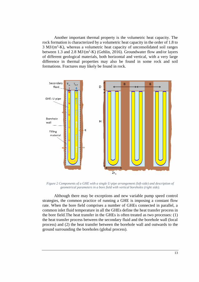
number of vertical and/or tilted boreholes with a regular or any arbitrary pattern.
The borehole diameter (2rb) normally varies between 0.075 and 0.180 m and
borehole depth have typically been ranging between 40 and 150 m for the vast
majority of the system in Europe. Lately, deeper boreholes are being drilled with
borehole length that ranges between 200 and 350 m. The uppermost meters of the
borehole (D) as shown in Figure 2, represents either the part above the
groundwater level and/or depth of an upper layer having much lower thermal
conductivity than the rest of the surrounding ground, typically varying between 2
and 8 m. The active total borehole length (H) is the total drilling length excluding
12
the upper inactive part. The spacing between boreholes is represented by B in
Figure 2, typically ranging between 3 and 6 m in thermally balanced GCHP/BTES
installations.
Widely used GHEs consist of either a single or a double U-shaped plastic
tube(s) with outer diameters between 32 and 50 mm and a wall pipe thickness that
varies between 2.0 and 3.7 mm. More efficient GHE designs such as co-axial types
are currently in a R&D phase (Acuña, 2013) and have already been tested on the
field at several sites achieving a technology readiness level of about 6.
As for the heat carrier fluid circulating within the GHEs, water is used as a
secondary fluid par excellence in many countries where the operation of the GCHP
system results in fluid temperatures remaining sufficiently far from the water
freezing point. However, operation of the GCHP system may result in fluid
temperatures near or below the water freezing point. In order to avoid freezing in
this situation, an aqueous solution of ethyl alcohol is commonly used to lower the
freezing point of the secondary fluid. In Sweden, 70-75% of the GCHP
installations use an aqueous solution of 20-25 wt-% ethyl alcohol with additionally
ca 2.5 wt% of some denaturing agents, e.g. 2 wt% isopropyl alcohol and ca. 0.5
wt% of n-butyl alcohol having a freezing point of ca. -15 C (Ignatowicz, 2016).
The space between the borehole wall and the GHE is filled to ensure the
heat transfer between the pipes, through which the secondary fluid circulates, and
the surrounding ground. In northern Europe, a common practice is to let the
natural groundwater be the filling material when no risks for mixing of different
groundwater qualities is identified. A grouting material consisting of a mixture of
different materials such as coarse sand, quartz, bentonite or graphite is utilized in
most other countries. Grouting materials are mainly used to prevent migration of
contaminants into the groundwater and mixing of different groundwater qualities.
The ground surrounding the GHEs constitutes the medium through which
the heat is exchanged, or in which the thermal storage is built-up. The composition
of the ground is particular to each location, which may be made up of geological
materials with either similar or dissimilar thermal properties. The thermal
conductivity of the geological materials ranges between 1 and 7 W/(m-K)
depending on the mineral composition (Sundberg, 1991). As reported in (Gehlin,
2016), a high thermal conductivity is desirable to have efficient heat transfer
between the ground and the GHEs.
13
Another important thermal property is the volumetric heat capacity. The
rock formation is characterized by a volumetric heat capacity in the order of 1.8 to
3 MJ/(m3-K), whereas a volumetric heat capacity of unconsolidated soil ranges
between 1.3 and 2.8 MJ/(m3-K) (Gehlin, 2016). Groundwater flow and/or layers
of different geological materials, both horizontal and vertical, with a very large
difference in thermal properties may also be found in some rock and soil
formations. Fractures may likely be found in rock.
Figure 2 Components of a GHE with a single U-pipe arrangement (left-side) and description of geometrical parameters in a bore field with vertical boreholes (right side).
Although there may be exceptions and new variable pump speed control
strategies, the common practice of running a GHE is imposing a constant flow
rate. When the bore field comprises a number of GHEs connected in parallel, a
common inlet fluid temperature in all the GHEs define the heat transfer process in
the bore field.The heat transfer in the GHEs is often treated as two processes: (1)
the heat transfer process between the secondary fluid and the borehole wall (local
process) and (2) the heat transfer between the borehole wall and outwards to the
ground surrounding the boreholes (global process).
14
2.1.2 Heat transfer inside the borehole
A convective-diffusive heat transfer process occurs at the GHEs. Heat
convection takes place between the fluid and the pipe wall, while the heat is
transferred by conduction through the pipe walls and the grouting material.
Convection also takes place outside the pipes in groundwater filled boreholes. The
heat transfer between the fluid and the borehole wall has been in some studies
approached as a quasi-steady process through the definition of thermal resistances.
The simple mean fluid temperature (Tf) and the borehole wall temperature
(Tbw) can be expressed as a relation between the effective fluid-to-borehole wall
thermal resistance (Rb∗) and the heat transfer rate per unit length (q), as expressed
in Equation 1.
Tf(t) = q(t) ∙ Rb∗ + T bw(t) (1)
The effective fluid-to-borehole wall thermal resistance (Rb∗) accounts for
the influence of fluid temperature variations along the borehole length and of the
transverse heat flow exchanged between the downward and upward pipes, referred
as thermal shunt flow. For high flow rates, thermal shunt flow on the conditions at
the borehole wall has been disregarded i.e. the average temperature over the depth
do not differ significantly from the simple mean temperature. However, the simple
mean fluid temperature differs from the avearge temperature over the borehole
length for small flow rates or long boreholes. In the latter case, the effective
borehole thermal resistance is larger than the borehole thermal resistance. A
number of research activities focused on developing methods to account for the
fluid temperature variation along the borehole length, as reported in (Zeng et al.,
2003), (Marcotte and Pasquier, 2008),(Lamarche, 2010), (Beier, 2011), (Beier and
Spitler, 2016) and (Lamarche et al., 2017).
Formulas of an equivalent borehole-to-fluid thermal resistance Rb* in
relation to local borehole thermal resistance were derived in (Hellström, 1991).
These formulas of Rb* were provided for both uniform temperature and uniform
heat flux conditions along the borehole. The local borehole thermal resistance (Rb)
refers to the borehole thermal resistance at an specific borehole depth, z, as (Rb)
as expressed in Equation 2.
Tf,z(t) = q(t) ∙ Rb + Tbw(t) (2)
where Tf,z is the local mean fluid temperature at a given depth z.
15
2.1.3 Heat transfer process in the ground
Modelling the thermal process in the ground taking into account all
possible particularities adds an extra level of complexity. Some of these conditions
(e.g. groundwater flow, rock or soil heterogeneity, factors above ground source
such as weather consition and human activities) affecting the heat transfer in the
ground can hardly be determined beforehand. For this reason and for the sake of
keeping a simple approach to the heat transfer process in the ground, the following
assumptions are often assumed:
The heat transfer process between the borehole wall and the surrounding
ground is treated as a pure conduction process.
The ground is considered as a homogeneous and isotropic medium, with
constant and temperature independent thermo-physical properties.
The initial temperature of the ground is known and equal to the
undisturbed ground temperature.
The boundary condition at the top surface and at the far outer boundary
of the surrounding ground are also set to the undisturbed ground
temperature.
The implications of these assumptions with respect to the heat transfer
process in the boreholes were investigated in several studies, as reviewed next.
As for the assumption of modelling the thermal process in the ground as a
pure heat conduction disregarding the effect of groundwater advection because of
natural groundwater movement, a negligible influence of the effect of a
unidirectional constant groundwater flow transversal to the longitudinal axis of the
borehole length and homogeneously spread under steady state condition in a
homogenous porous medium was reported in (Eskilson, 1987). Lately, several
investigations focused on developing mathematical models to take into account
the groundwater advection as reported in (Al-Khoury et al., 2005; Al-Khoury and
Bonnier, 2006; Al-Khoury et al., 2010; Diersch et al., 2011a; Diersch et al., 2011b;
Dehkordi et al., 2015 and Rivera et al. 2015 and 2016). In general, models based
on pure heat conduction process result in more conservative solutions as compared
to models including groundwater advection. (Dehkordi et al., 2015b) carried out
an analysis for different bore field configurations with and without groundwater
advection. Results pointed out that groundwater movement was less sensitive to
cases with balanced load; whereas, groundwater flow might have a comparable
impact on the borehole-to-borehole spacing when load condition was imbalanced.
16
Preliminary results on BTES systems have shown that the BTES storage capability
was deteriorated due to groundwater flow (Dehkordi et al., 2015b).
On the other hand, the effect of groundwater flow in both horizontal and
vertical fractures in rocks on the heat transfer in the ground was also investigated
for a given ground load condition and small bore field configurations in (Dehkordi
et al. 2015a). Thermal plumes and fluid temperatures were shown to be mainly
affected by the distance and by the number and the aperture when vertical and
horizontal fractures, respectively, occurs at the proximity of the borehole
As for the hypothesis of homogenous and isotropic ground medium,
(Ingersoll L. and Plass J., 1948) defined the ground surrounding the bore field as
a single homogenous layer with constant average thermal properties.This has been
a common practice in engineering to disregard the effect of various layers and to
define a single homogenous layer with an average effective thermal conductivity.
The effective thermal conductivity of the ground can be measured with a
traditional Thermal Response Test (TRT). However, the ground is made up of
various stratified geological materials with different thermal properties. The
influence of a multilayer ground in fluid temperature predictions was also subject
to a study, as presented in (Sutton et al., 2002 and Lee, 2011). Regarding the
assumption of a homogenous ground, (Eskilson, 1987) reported a small
temperature difference, less than 0.04 C, when solutions resulting from numerical
simulations with a two-layered soil (k= 2.5 W/(m-K) for z varying between 0 and
D+H/2 and k= 4.5 W/(m-K) for z > D+H/2) were compared with the
corresponding homogeneous case with k= 3.5 W/(m-K). Thermal conductivity of
the ground in-situ can, among others, be measured through Distributed Thermal
Response Test (DTRT) as reported in (Fujii, 2006 and Acuña, 2013).
Regarding the initial condition in the ground domain, in (Eskilson, 1987),
the effect of the geothermal heat flux was simplified to a constant temperature
value defined by the effective undisturbed ground temperature. Studies were also
performed to assess the influence of this assumption, as explained next. The
effective undisturbed ground temperature resulted from the assumption that at the
top surface the temperature of the ground is set as the annual average air
temperature, then the temperature along the borehole depth increases linearly from
the top surface and with depth according to a given geothermal gradient. So that,
the effective undisturbed ground temperature is set as a constant temperature value
equal to the undisturbed mean temperature along the borehole depth. The influence
of the geothermal heat flux was assessed by computing the isotherms at the
surrounding ground after 25 years considering the geothermal gradient and the
aforementioned assumption. The comparison of both studies showed that the
17
borehole wall temperature deviated only 0.01 C, which was considered as a
negligible error.
As for the condition at the top surface, research studies also focused on the
evaluation of factors such as outdoor air temperature variations (daily and yearly),
snow, heat flux due to either heat extraction in the borehole or existing buildings
with regards to the assumption of a constant temperature boundary condition, as
reviewed next.
The penetration depth, as defined in (Eskilson, 1987 and thereafter in
Hellström, 1991), was used as an indicator of the magnitude of the disturbances in
the top part of the ground due to the outdoor air temperature variation. For
example, the penetration depth due to a periodic annual temperature variation
corresponds to only a few meters, which is around 4 m when the ground thermal
diffusivity α=1.62×10⁻⁶ m2/s (value reported in Eskilson’s examples). As
compared to a borehole length of 100 m, the effect of this disturbance, occurring
in the top few meters, was assumed to be negligible in (Eskilson, 1987).
Recently, the influence of the outdoor air temperature on the outlet fluid
temperature has been assessed via three different assumptions: time and space
varying ground temperature, uniform time varying ground temperature, and
constant ground temperature (Cimmino, 2017). The differences in the outlet
temperature predictions is assessed for steady state conditions and taking into
account the penetration depth in relation to the inactive and the active parts of the
borehole. The analysis is applied to a large number of bore field configurations
with series connection. Results showed that the prediction of the outlet fluid
temperature assuming a ground constant temperature results in a small deviation
(less than 0.1K) as compared to the case with a time and space varying ground
temperature for typical lengths of vertical boreholes. But, short boreholes may be
significantly affected by the air outdoor temperature variations.
(Rivera et al. 2016) pointed out that the influence of outdoor air
temperature is negligible for sufficiently deep boreholes when the boundary
condition at the top surface is represented as a constant temperature, with less than
5% deviations on mean borehole wall temperature predictions for boreholes
deeper than 50 m. The differences decrease with the increasing of the borehole
depth. However, shallow boreholes may be affected significantly by the variations
of the boundary condition at the top surface.
The influence of the thermal disturbance at the top surface due to heat
extraction in the borehole was also evaluated in (Eskilson, 1987). Numerical
examples for the case of a single borehole with rb=0.005 m, H=110 m, D=5 m and
18
α=1.62×10⁻⁶ m2/s and an annual heat extraction of 21000 kWh/year showed that
its effect was small (68% of the heat comes from the borehole with only 32% from
the surface at the 25th year of operation) and the disturbance at the top surface was
assumed to be negligible. Lately, the definition of a constant temperature boundary
condition at the top surface of the ground has been an issue of discussion as it may
not represent accurately the thermal process in the near vicinity of the boreholes
at the top surface. (Rivera et al. 2015 and 2016) have recently developed models
which can be applied to investigate the effect of heat flux through the top surface
due to a variety of scenarios because of different land-use.
As reviewed above, research community is devoting an extensive effort on
the development of modelling tools capable to capture the ground particularities
to a large extent. In this Ph.D. study, the investigations are focused on vertical
boreholes with active borehole lengths >100 m, which have been proved not to be
significantly affected by the aforementioned ground particularities. Besides,
solutions based on the above assumptions, , have been demonstrated to model the
response of the ground within acceptable margin, as shown in reference studies
presented in (Eskilson, 1987 and Hellström, 1991). In this Ph.D. work, the heat
transfer in the ground has been modelled according to the assumptions listed
above.
Under these assumptions, the temperature field in the ground is derived
from the heat diffusion equation in a differential control volume as a function of
time at a given point. The heat conduction rate is evaluated by Fourier’s law. Thus,
temperature distribution in Cartesian coordinates at a point T(x, y, z) as a function
of time is expressed as in Equation 3:
∂
∂x(k
∂T
∂x) +
∂
∂y(k
∂T
∂y) +
∂
∂z(k
∂T
∂z) = ρcp
∂T
∂t (3)
According to the hypothesis of a homogeneous medium, Equation 4 can be
written as expressed in Equation 4, with 𝛼 as the thermal diffusivity, α = k/(ρcp).
∂2T
∂x2 +∂2T
∂y2 +∂2T
∂z2 =1
α
∂T
∂t (4)
A set of equations defining the initial and boundary conditions in the
domain, as listed above, are used to find a single solution to this physical problem.
The temperature field can be solved using both analytical and numerical methods.
Analytical methods provide mathematical expressions; however, exact solutions
are often limited to simple geometries. In numerical methods, the domain is
discretized in nodes or sub-domains, and the differential partial equations defining
the temperature field are approximated by simpler expressions to find the solution
19
easily. Both analytical and numerical solutions have been proposed to solve the
heat transfer process in multiple GHE bore fields. Nowadays progress of
computing technology has favored the development of software programs capable
of finding numerical and semi-analytical solutions of complex problems, as
reviewed next.
2.1.4 Solutions to the heat transfer process in the
ground
The first reference studies on GHE modelling in multiple bore fields were
carried out by Per Eskilson during his Ph.D. studies (Eskilson, 1987) under the
supervision of Prof. Johan Claesson. Despite the limited computational capability
of computers at that time, solutions based on Eskilson’s and Claesson’s studies
were developed with such a precision level that they are still used. During
Eskilson’s Ph.D. studies, both analytical and numerical approaches were
investigated and proposed to provide solutions to the ground temperature field
response, according to Equation 4 and under the assumptions listed in Chapter
2.1.3.
The superposition borehole model (SBM) (Eskilson, 1986) is a 3-D
numerical model based on the finite difference method, utilized to obtain formulas
to relate the heat extraction rate and the temperature at the borehole wall, being
reported in (Eskilson, 1987). In the SBM the response of a single borehole is
modeled according to prescribed conditions that define the heat transfer process in
the GHE and with the ground, as discussed next, that were selected by the user.
Besides, the mirror technique was used to define a constant temperature at the top
surface. The mirror technique consists of superimposing the temperature field of
the single borehole to a symmetric temperature field with opposite sign. The SBM
was capable to model the response of multiple bore fields by applying temporal
and spatial superposition of the single borehole.
As mentioned above, the SBM could also be used to define different
boundary conditions to represent the heat transfer process between the fluid and
the ground. Among these definitions, there was one in which the heat transfer
process inside the GHE was modeled as a thermal resistance circuit and coupled
with the ground. Besides this detailed formulation, the SBM also included some
other formulations in which the heat transfer process in the surrounding ground
was decoupled from the heat transfer inside the GHE, as explained in this chapter.
In these decoupled formulations the heat transfer process inside the GHE was
approximated through the definition of a boundary condition at the borehole wall,
which was representing the heat transfer process between the fluid and the ground
20
at the borehole wall. A discussion and analysis of the heat transfer process
occurring at the borehole wall are provided in this dissertation, in Chapter 2.2.
Besides the SBM, (Eskilson, 1987) also proposed the finite line source
(FLS) as an analytical method to model the ground thermal response with GHEs.
Previous to the FLS approach, the infinite line source (ILS) (Ingersoll and Plass,
1948) and the cylindrical heat source (CHS) (Carslaw and Jaeger, 1947)
approaches were used to model the thermal response of a single GHE as a line and
as a hollow cylinder, respectively, in an infinite medium. Whereas both ILS and
CHS approaches were limited to model the heat transfer in the ground as a 2-D
radial process, the FLS approach was also able to capture axial heat transfer
effects.
The FLS is derived from the point source expression (Carslaw and Jaeger
in Chapter 10, 1947) extended over a finite line, H, as the active borehole length,
located at a distance D from the top surface (see Figure 2), as inactive upper part
of the borehole, in a semi-infinite medium. The constant temperature at the top
surface was set using the mirror technique. For multiple bore fields, the FLS
solution results in a double integral in the space domain that converts in a triple
integral when evaluated for multiyear response (simple integral in the time
domain).
(Eskilson, 1987) used the SBM approach with a uniform temperature
boundary condition to model the heat transfer process in the ground, discussed in
Chapter 2.2., rather than the FLS analytical approach to provide formulas for the
relation of the heat extraction rate and the borehole wall temperature. However,
no reflection was found about his preference here. The reason for his preference
was probably limitations of the FLS approach to accurately approximate the heat
transfer process between the borehole wall and the surrounding ground and of
computing capacity to solve the (triple) integral expression for the transient state.
The integral solution requires numerical algorithm solutions that were impractical
due to the long computing time needed for the evaluation of a triple integral
expression in both space and time domain.
After (Eskilson, 1987), main efforts on this subject were focused on
overcoming the limitation of the FLS approach to find the exact solution. First,
(Zeng et al., 2002) proposed to evaluate the integral at mid-height of the borehole
depth. Next, (Lamarche and Beauchamp, 2007) proposed a simplification of the
integral, converting the integration from a triple to a double integral expression,
making it computationally faster and showed that the evaluation at mid-height
resulted in higher values. Later, (Claesson and Javed, 2011) simplified the double
21
integral of the space domain to a simple integral of the complementary error
function.
At the time that this Ph.D. study was initiated, the computational limitation
of the FLS approach were already solved. However, the comparison of solutions
from approaches based on the FLS against the SBM solution included in (Eskilson,
1987) showed that the FLS analytical approach overestimated the response.
Extensive investigations have been carried out during the time of this Ph.D. study
on this topic, providing a comprehensive understanding of the FLS approach with
respect to the investigations reported in (Eskilson, 1987). Undoubtedly, the
investigations done by Claesson and Eskilson were the foundation of modelling
GHEs.
2.2 Boundary conditions in mathematical modelling of
GHEs connected in parallel
This chapter reviews the definition of the heat transfer process between the
GHE and the surrounding ground that have been applied in mathematical models
through the definition of the boundary condition at the borehole wall, after
(Cimmino and Bernier, 2014). Categorization of the different boundary conditions
were also tackled in the SBM (Eskilson, 1986). (Cimmino and Bernier, 2014 and
Spitler and Bernier, 2016) have recently built up a complete understanding of the
heat transfer process with regard to the definition of boundary conditions in GHE
modelling and connected them with the limitation of pure FLS approaches.
2.2.1 Constant heat flux at the borehole wall in all
boreholes
Mathematical models based on a constant heat flux boundary condition
assume that the total heat flow is distributed equally to all the boreholes and
uniformly distributed along the borehole length.
With the condition of a constant heat flux at the borehole wall in all the
boreholes, temperature response along the borehole depth is not uniform,
presenting gradients at regions next to borehole edges and with larger values at the
top edge region. The temperature at the borehole wall in the inner borehole is
higher than in the outer boreholes. The average borehole wall temperature differs
from borehole to borehole, being higher in the boreholes in the central part of the
bore field. Mathematical models based on this assumption are described in the
SBM – LOMODE =1 (Eskilson, 1986), (Lamarche and Beauchamp, 2007 and
Claesson and Javed, 2011).
22
2.2.2 Equal average borehole wall temperature in all
boreholes
Some solutions were developed to account for the heat flow distribution
among the boreholes within the bore field by setting the condition that the average
borehole wall temperature is the same in all the boreholes and that the sum of the
heat flow in all boreholes is equal to the total thermal power imposed in the bore
field. In these solutions, the heat is distributed uniformly along the borehole wall
of each borehole, but the heat flows are different between the boreholes. Boreholes
with similar surrounding conditions have the same heat flow. Approaches based
on this assumption are reported in the SBM – (LOMODE= 2) (Eskilson, 1986),
(Cimmino, 2013 and Lazzarotto, 2014).
2.2.3 Uniform borehole wall temperature in all boreholes
Some other models are based on the assumption that at a high volume flow
rate in U-pipe heat exchangers the temperature change along the pipe is expected
to be small so that the average fluid temperature can be assumed to be uniform
along the borehole depth. On the basis of this assumption, the temperature at the
borehole wall is extrapolated to be uniform also along the borehole length.
Thus, a uniform borehole wall temperature condition is fulfilled in all
boreholes in multiple bore fields. Besides, the sum of the heat flow distributed to
each borehole is equal to the total heat flow imposed in the bore field.
Mathematical models based on this boundary condition are presented in the SBM
–(LOMODE =3) (Eskilson, 1986), (Cimmino and Bernier, 2014 and
Lazzarotto, 2016).
2.2.4 Same inlet fluid temperature in all boreholes
This section reviews mathematical models focused on more detailed
development based on same inlet temperature boundary conditions in all the
boreholes.
(Lee and Lam, 2008) proposed a 3D implicit FDM that modeled the heat
transfer inside the borehole with a 3D FDM under a quasi-steady state condition
and the heat transfer in the surrounding ground was also modeled with a 3D FDM
with a rectangular coordinate system in which square columns represent the
boreholes. These two solutions were coupled and solved iteratively at each time
step. Fluid temperatures along upward and downward pipe flows were modeled.
The temperature profile at the borehole wall along its length showed that its
23
maximum temperature in heat injection was observed near the top, which is further
discussed in Chapter 2.2.5.
(Cimmino, 2015) proposed a semi-analytical solution that accounts for the
axial variation of the temperature and the heat rates at the borehole wall because
of the thermal interaction between the fluid and the borehole wall. The model was
used to perform simulation of the response of a single U-pipe GHE in the cases of
a single and multiple bore fields with parallel GHEs connection. In this model, an
analytical approach of the heat transfer process between the fluid and the borehole
wall was coupled to the system of equations that solve the temperature and heat
transfer rate at the borehole wall, which was based on (Cimmino and Bernier,
2014). This model provided the temperature response of the ground for an equal
inlet fluid temperature condition in all the boreholes. The effect of the GHE
thermal resistance and fluid flow rate in the temperature response factors were
studied for a total constant heat flow. Results about this investigation are further
discussed in Chapter 2.3.1.
Recently, (Cimmino, 2016) extended the model developed in (Cimmino,
2015) for different piping arrangements (independent U-tubes, parallel and series)
in a single borehole. For a parallel connection of a double U-pipe arrangement for
heat extraction, the minimum borehole wall temperature was observed near the
top, as discussed in the next sub-chapter.
Regarding numerical modelling, (Ozudogru et al., 2014) proposed a
numerical model based on FEM where the GHE (single U-pipe) was modelled as
a 1D finite element representation and coupled to 3D elements that model the heat
transfer in the surrounding ground as a pure heat conduction process. Some
computational errors were reported when coupling 1D and 3D elements, which
were overcome with the assistance of a pseudo-pipe. Temperature response are
shown for short-term calculations, showing a good agreement with the FLS
solution.
2.2.5 Discussion about boundary conditions and its
relation to this work
Approaches based on the boundary conditions described above have been
accepted for modelling the thermal response of the ground. However, researchers
proved that the use of models based on constant heat flux result in an
overestimation of the bore field temperature response, which increases with time
and the number of boreholes, as shown in (Lee and Lam, 2008 and Fossa, 2011).
Differences between models based on constant heat flux as compared to models
24
described by a uniform borehole wall temperature are due to the limitation of the
former to represent the heat flux distribution properly along the borehole.
The assumption of a uniform heat flux distribution causes concealed errors
on the accurate calculation of the thermal interaction between boreholes and on
the heat flow distribution among the boreholes. To overcome this limitation,
boundary conditions were reformulated with an equal average borehole wall
temperature in all boreholes at every given time, to correct the heat flow
distribution among the boreholes. Although significant improvements were
achieved in models based on this, as reported in (Cimmino et al., 2013), the
assumption of a uniform heat flux distribution along the borehole length did not
adequately represent the thermal behavior of the ground, which also resulted in a
misconception of the heat flow distribution among the boreholes.
Models based on a uniform borehole wall temperature are still preferred for
modelling the thermal response of the ground. The solution proposed by (Eskilson,
1987), which is based on this, has been used as a benchmark during the last three
decades.
(Cimmino and Bernier, 2014) proposed a semi-analytical solution in which
the borehole is modeled as a series of segments. The uniform temperature
condition at the borehole wall is fulfilled with the definition of an equal
temperature in all the segments and in all the boreholes at every given time. The
borehole wall temperature at each segment is calculated from the spatial and
temporal superposition of the FLS solution. The approach proposed by (Claesson
and Javed, 2011) is used in this study to calculate the response of each segment.
The Laplace transform is used to solve the time-varying heat load. The variation
of the heat rate is accounted for among the boreholes and along their depth which
is uniformly distributed along the length of each segment. This approach is
employed to model boreholes with different lengths and buried depths. This model
was implemented in the Pre-processor (Cimmino and Bernier, 2013), a graphical
user interface (GUI) in Matlab, that generates the thermal response factor (see
Chapter 2.3) for all three boundary conditions described above. The Pre-processor
has been particularly useful for the investigation presented in this dissertation.
A similar procedure of dividing the borehole into segments and calculating
the temperature response of each segment to fulfill a uniform temperature
boundary condition at the borehole wall was used by (Lazzarotto, 2016) to model
vertical and inclined boreholes. (Lazzarotto, 2016) employed the FLS
approximation developed by (Lamarche and Beauchamp, 2007) and applied
simplifying algorithms to make the computing time efficient.
25
The model proposed in Paper 1 was utilized to deepen the understanding
of the response of the ground at the borehole wall when the temperature drop along
the GHE is negligible and the borehole thermal resistance is neglected.
Although the formulation of the heat transfer process in the ground based
on the uniform borehole wall temperature boundary condition is widely accepted,
it requires a deeper discussion. The first aspect of this discussion is that the
assumption of uniform borehole wall temperature at the borehole wall deviates
from the original formulation with a uniform fluid temperature. The existing
thermal resistance between the fluid and the borehole wall and the increase of the
heat flux at the borehole ends causes the borehole wall temperature to deviate from
the assumption of uniform temperature, as shown in Figure 3. Paper 2 introduced
a correction on the definition of the heat transfer process occurring at the GHE that
accounts for the thermal interaction between the fluid and the borehole wall, i.e.
the GHE thermal resistance, using a thermally resistive layer at the borehole wall
with a given thermal conductivity.
The second subject for discussion is the statement of uniformity of the fluid
temperature along the borehole depth. It is often assumed that the arithmetic
average of the inlet and outlet fluid temperature corresponds to the average fluid
temperature along the borehole length (as presented in equations 1 to 3). This
statement is valid under the assumption of a sufficiently high flow rate so that axial
change of the fluid temperature is neglected, i.e. the change of the fluid
temperature along upward and downward pipes is small (Eskilson, 1987). It also
implies that differences between the effective thermal resistance and local thermal
resistance are negligible. Differences between these resistances have been
experimentally demonstrated in (Acuña, 2013).
As pointed out in Chapter 2.1.2, the thermal shunt flow occurring between
the upward and downward legs of the pipes implies that the averaged-over-the
depth mean fluid temperature deviates from the simple mean fluid temperature.
So, the effective borehole thermal resistance is recommended to be used to capture
this effect.
Some research studies have shown that the thermal shunt increases with
borehole length, conductance between pipe-legs, decreasing flow rate (Beier,
2011; Javed and Spitler, 2016 and Beier and Spitler, 2016) and is larger for coaxial
heat exchangers (Acuña, 2013) when the central pipe is not insulated.
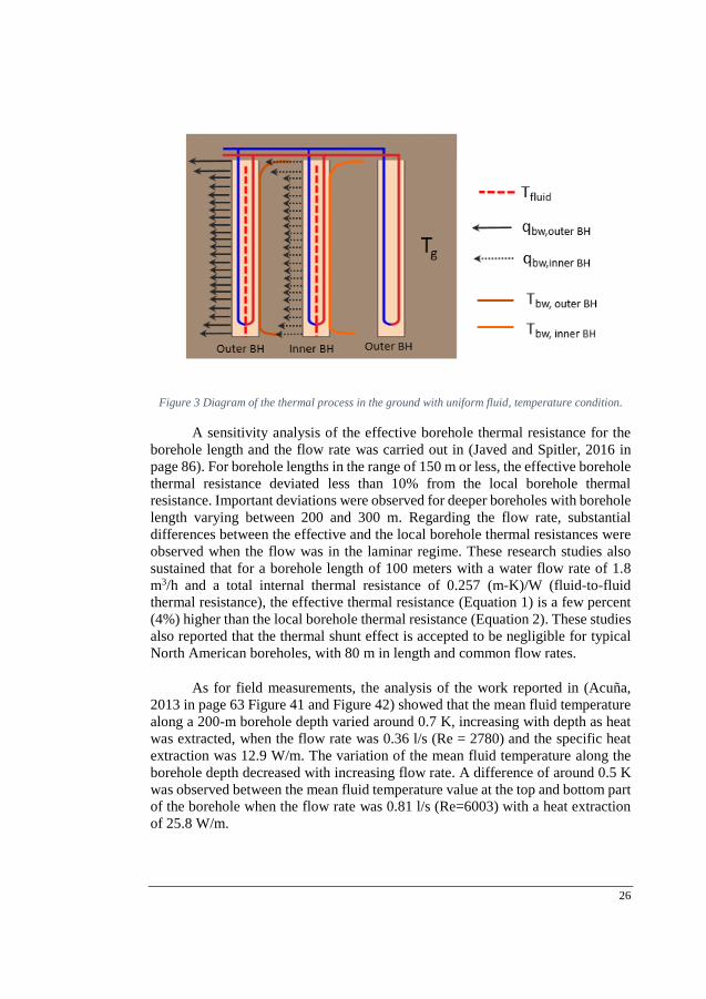
26
Figure 3 Diagram of the thermal process in the ground with uniform fluid, temperature condition.
A sensitivity analysis of the effective borehole thermal resistance for the
borehole length and the flow rate was carried out in (Javed and Spitler, 2016 in
page 86). For borehole lengths in the range of 150 m or less, the effective borehole
thermal resistance deviated less than 10% from the local borehole thermal
resistance. Important deviations were observed for deeper boreholes with borehole
length varying between 200 and 300 m. Regarding the flow rate, substantial
differences between the effective and the local borehole thermal resistances were
observed when the flow was in the laminar regime. These research studies also
sustained that for a borehole length of 100 meters with a water flow rate of 1.8
m3/h and a total internal thermal resistance of 0.257 (m-K)/W (fluid-to-fluid
thermal resistance), the effective thermal resistance (Equation 1) is a few percent
(4%) higher than the local borehole thermal resistance (Equation 2). These studies
also reported that the thermal shunt effect is accepted to be negligible for typical
North American boreholes, with 80 m in length and common flow rates.
As for field measurements, the analysis of the work reported in (Acuña,
2013 in page 63 Figure 41 and Figure 42) showed that the mean fluid temperature
along a 200-m borehole depth varied around 0.7 K, increasing with depth as heat
was extracted, when the flow rate was 0.36 l/s (Re = 2780) and the specific heat
extraction was 12.9 W/m. The variation of the mean fluid temperature along the
borehole depth decreased with increasing flow rate. A difference of around 0.5 K
was observed between the mean fluid temperature value at the top and bottom part
of the borehole when the flow rate was 0.81 l/s (Re=6003) with a heat extraction
of 25.8 W/m.
27
(Lee and Lam, 2008) developed a 3D FDM model, that coupled the GHE
and the surrounding ground, to obtain the temperature profiles of the fluid along
upward and downward pipes and of the borehole wall for a single borehole
(rb/H=0.0005) under continuous heat injection for a 10 year-period. In this study,
after 1 year, the maximum temperature at the borehole wall occurred near the top
edge of the borehole, which was contrary to the maximum value observed at mid-
height borehole resulting from a pure FLS solution. Besides the edge effect at
borehole ends, a temperature gradient of 0.2 K was observed in the temperature
profiles along the borehole wall after 1 year with continuos heat injection. With
regard to the fluid temperature profiles, the mean fluid temperature resulting from
the average fluid temperature at the at the upward and downward pipes at the top
and the bottom part of the GHE showed a slight temperature gradient of around
0.7 K, as read out from the results presented in (Lee and Lam, 2008). Temperature
profiles were only presented for the case of a single borehole. Average borehole
wall temperatures for few multiple bore fields after 10 years resulting from the
numerical solution were also reported in (Lee and Lam, 2008).
(Cimmino, 2016) studied the temperature profiles of the fluid at the
downward and upward pipes and at the borehole wall after 10 years of continuous
heat extraction for various GHE connections (independent, parallel and series U-
pipes) in a single borehole (rb=0.075 m, H=100 m and D=2 m). For the case of 4
U-pipes with parallel connection with given geometrical aspect ratios and a fluid
flow rate of 0.2 kg/s, the analysis of the temperature variation along the borehole
depth between the downward and upward fluid temperature profiles showed that
its average value resulted in a small temperature change along the borehole depth,
being less than 0.1 K and increasing with depth as heat was extracted. At the
borehole wall, apart from the edge effects at the top and bottom part of the
borehole, a similar behavior was observed for the temperature gradient along the
borehole depth, being less than 0.1 K and increasing with depth as heat was
extracted.
As supported by these theoretical and observational investigations, the
variation of the mean fluid temperature along the borehole depth may be small for
some conditions. Therefore, the assumption of a uniform fluid temperature along
the borehole depth can be accepted as representative for typical U-pipe GHEs,
typical borehole lengths and high flow rates (high enough to ensure Re>2300, i.e.
turbulent flow, for given geometry of the GHE and for given physic properties of
the secondary fluid).
The investigations presented in Paper 2 were carried out for small and
medium sized bore fields with borehole lengths varying between 48 and 150 m
and under the assumption that the flow rate was high. For these circumstances, the
28
assumption of a uniform mean fluid temperature along the borehole length was
accepted as a good representation of the conditions in the GHE. The potential of
the model developed during this Ph.D. work was also demonstrated in (Righi,
2013) for the single borehole to model the response of the ground when the mean
fluid temperature presents a gradient along the borehole length.
2.3 Simulation of ground temperature response and bore
field sizing methods
Mathematical models provide practitioners with a better understanding of
the thermal process in the ground. Characterization of the thermal properties of
the ground and bore field sizing are most common applications of mathematical
models.
The ground is characterized by a given heat capacity and thermal
conductivity, which depends on thermal properties of the geological formation at
a site. Besides, the heat transfer process of the ground in borehole fields presents
a transient response in the order of years or decades. Because of these two aspects,
multi-year simulations of ground response are required for given estimated
thermal loads at the heat pump. Therefore, the ground response should be
investigated with relation to the bore field layout, number of boreholes and the
geometrical aspect ratios of the bore field in order to ensure that the temperature
of the fluid circulating inside the GHEs is kept within the operational limits during
the lifetime of the GCHP system (20-25 years). It is important to note that the
lifetime of GHEs is normally much longer than of the overall GCHP system.
In this dissertation, two well-known bore field sizing methods are
investigated: the method based on the generation of the relevant g-function for a
bore field, and the ASHRAE method. Both methods are based on an iterative
procedure, in which the total length of the active boreholes (nb × H), i.e. total bore
field length, is adapted to fulfill operating fluid temperature constraints of the heat
pump. The former method consists of a sequential superposition of the stepwise
variable loads over the g-function, the characteristic temperature response of the
bore field. Therefore, the accuracy on the g-function generation has a direct
connection with the accuracy of the representation of the response of the bore field.
The models proposed in Paper 1 and 2 were utilized to discuss the response of the
ground according to the g-function concept and with regard to the boundary
conditions defined in the mathematical approaches of reference solutions. In the
latter, the ASHRAE method, the ground load condition is defined as three
consecutive steps strictly defined as a monthly component when the worst peak
load condition occurs, the peak load itself and an annual load based on a 10-year
simulation. The robustness of this method to calculate the total bore field length at
29
any other duration, apart from 10-year, is reviewed The ASHRAE method
provides also the foundation of the methodology proposed in Paper 3. The
methodology developed in Paper 3 is applied to investigate the optimum borehole
spacing on a particular case with quasi-balanced load, in which the annual net
ground load condition is virtually zero.
2.3.1 The g-function
Several mathematical approaches, which were reviewed in Chapter 2.2,
have been used to generate the g-function. During the last decades, the research
community efforts have been focused on providing a complete knowledge of the
heat transfer process and the g-function concept.
The g-functions was the result of Eskilson’s final goal in his studies
(Eskilson, 1987). The g-function is the non-dimensional temperature response
factor that relates the change in temperature over time at the borehole wall from
its undisturbed value when a total constant heat load Q (W) (Q = nbHq) is
injected into the bore field, where q represents the average heat extraction per unit
borehole length (W/m) and nb the number of boreholes. The g-function is
mathematically defined in Equation 5:
Tbw − Tg =q
2πkg (
t
ts,
rb
H,
B
H,
D
H) (5)
The g-function1 is expressed as a function of non-dimensional parameters
that account for the bore field geometry and time. The non-dimensional time t
ts is
expressed as an aspect ratios of the characteristic time ts =H2
9αwhere α is the
thermal diffusivity of the ground. For example, the characteristic time corresponds
to 22 years for a borehole length of 100 m and the ground thermal diffusivity of
1.6210-6 m2/s. The characteristic parameters of bore field geometry: rb, B, D are
expressed as geometrical aspect ratios to H.
The SBM with uniform borehole wall temperature condition, as discussed
in Chapter 2.1.4, was utilized to generate the g-function for hundreds of bore field
geometries. The library of g-function is still used with current design tools and has
until a few years ago served as a benchmark. The linear nature of the heat transfer
problem of GHEs also allows to apply temporal superposition over the g-function,
1 The g-function can be easily generated from preprocessor (Cimmino and Bernier, 2013).
30
to any loading condition, as expressed in Equation 6, with a minimal computing
time:
Tbw(t) − Tg =1
2πk∗ (q1 ∗ g (
t
ts ,
rb
H,
B
H,
D
H) − qn ∗ g (
(t−tn)
ts,
rb
H,
B
H,
D
H) +
+ ∑ (qi+1 − qi) ∗ gn−1i=1 (
(t−ti)
ts,
rb
H,
B
H,
D
H)) (6)
Because of its practicability, this procedure (g-function + temporal
superposition) is widely used to predict temperature response for variable loading
condition and is used in design bore field commercial software programs, such as
Earth Energy Designer (Hellström and Sanner, 1994) and Ground Loop Heat
Exchanger Professional (Marshall and Spitler, 1994).
Although the SBM included a scrutinized procedure with several ways to
approach the heat transfer in the ground, lack of comprehensive understanding
may be the reason why the relevance of the boundary condition was disregarded
up to some years ago. A comprehensive categorization of the various types of
boundary conditions defined at the borehole wall has been provided by (Cimmino
and Bernier, 2014 and Spitler and Bernier, 2016). The heat transfer process in the
ground was characterized on the g-function response in (Cimmino et al. 2013).
This characterization included four different regions. The first region corresponds
to the response when the heat is transferred radially. The second region is
recognized when the thermal interaction between the boreholes starts. The time at
which this second region starts depends on (B
H), and it can be identified from the
comparison with the g-function of the single borehole. The third is defined when
t > 0.1 ∙ ts at which the heat transfer is a 2D (radial and axial) process. The last
part of the curve, when t > 10 ∙ ts, is defined as the fourth region with steady-state
conditions.
As mentioned above in Chapter 2.2, (Cimmino and Bernier, 2014)
developed a semi-analytical approach to overcome limitations of pure FLS
solution and to represent a uniform borehole wall temperature. g-Function
solutions from this approach showed good agreement with the g-function resulting
from Eskilson’s approach. The results obtained from the numerical model
described in Paper 1 were compared with both the g-function obtained from
Eskilson and the semi-analytical solution proposed by (Cimmino and Bernier,
2014).
The model developed by (Cimmino, 2015) was used to investigate the
effects of non-dimensional internal short-circuit conductance, non-dimensional
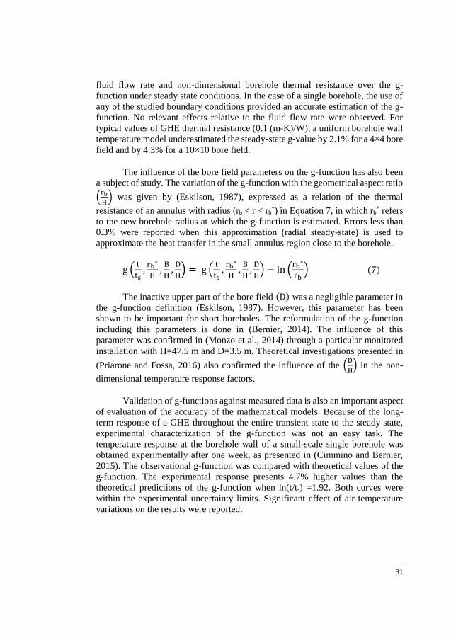
31
fluid flow rate and non-dimensional borehole thermal resistance over the g-
function under steady state conditions. In the case of a single borehole, the use of
any of the studied boundary conditions provided an accurate estimation of the g-
function. No relevant effects relative to the fluid flow rate were observed. For
typical values of GHE thermal resistance (0.1 (m-K)/W), a uniform borehole wall
temperature model underestimated the steady-state g-value by 2.1% for a 4×4 bore
field and by 4.3% for a 10×10 bore field.
The influence of the bore field parameters on the g-function has also been
a subject of study. The variation of the g-function with the geometrical aspect ratio
(rb
H) was given by (Eskilson, 1987), expressed as a relation of the thermal
resistance of an annulus with radius (rb < r < rb*) in Equation 7, in which rb
* refers
to the new borehole radius at which the g-function is estimated. Errors less than
0.3% were reported when this approximation (radial steady-state) is used to
approximate the heat transfer in the small annulus region close to the borehole.
g (t
ts,
rb∗
H,
B
H,
D
H) = g (
t
ts,
rb∗
H,
B
H,
D
H) − ln (
rb∗
rb) (7)
The inactive upper part of the bore field (D) was a negligible parameter in
the g-function definition (Eskilson, 1987). However, this parameter has been
shown to be important for short boreholes. The reformulation of the g-function
including this parameters is done in (Bernier, 2014). The influence of this
parameter was confirmed in (Monzo et al., 2014) through a particular monitored
installation with H=47.5 m and D=3.5 m. Theoretical investigations presented in
(Priarone and Fossa, 2016) also confirmed the influence of the (D
H) in the non-
dimensional temperature response factors.
Validation of g-functions against measured data is also an important aspect
of evaluation of the accuracy of the mathematical models. Because of the long-
term response of a GHE throughout the entire transient state to the steady state,
experimental characterization of the g-function was not an easy task. The
temperature response at the borehole wall of a small-scale single borehole was
obtained experimentally after one week, as presented in (Cimmino and Bernier,
2015). The observational g-function was compared with theoretical values of the
g-function. The experimental response presents 4.7% higher values than the
theoretical predictions of the g-function when ln(t/ts) =1.92. Both curves were
within the experimental uncertainty limits. Significant effect of air temperature
variations on the results were reported.
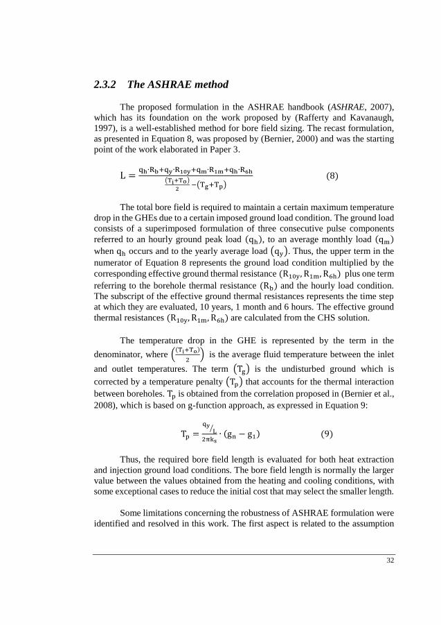
32
2.3.2 The ASHRAE method
The proposed formulation in the ASHRAE handbook (ASHRAE, 2007),
which has its foundation on the work proposed by (Rafferty and Kavanaugh,
1997), is a well-established method for bore field sizing. The recast formulation,
as presented in Equation 8, was proposed by (Bernier, 2000) and was the starting
point of the work elaborated in Paper 3.
L =qh∙Rb+qy∙R10y+qm∙R1m+qh∙R6h
(Ti+To)
2 −(Tg+Tp)
(8)
The total bore field is required to maintain a certain maximum temperature
drop in the GHEs due to a certain imposed ground load condition. The ground load
consists of a superimposed formulation of three consecutive pulse components
referred to an hourly ground peak load (qh), to an average monthly load (qm)
when qh occurs and to the yearly average load (qy). Thus, the upper term in the
numerator of Equation 8 represents the ground load condition multiplied by the
corresponding effective ground thermal resistance (R10y, R1m, R6h) plus one term
referring to the borehole thermal resistance (Rb) and the hourly load condition.
The subscript of the effective ground thermal resistances represents the time step
at which they are evaluated, 10 years, 1 month and 6 hours. The effective ground
thermal resistances (R10y, R1m, R6h) are calculated from the CHS solution.
The temperature drop in the GHE is represented by the term in the
denominator, where ((Ti+To)
2) is the average fluid temperature between the inlet
and outlet temperatures. The term (Tg) is the undisturbed ground which is
corrected by a temperature penalty (Tp) that accounts for the thermal interaction
between boreholes. Tp is obtained from the correlation proposed in (Bernier et al.,
2008), which is based on g-function approach, as expressed in Equation 9:
Tp =qy
L⁄
2πks∙ (gn − g1) (9)
Thus, the required bore field length is evaluated for both heat extraction
and injection ground load conditions. The bore field length is normally the larger
value between the values obtained from the heating and cooling conditions, with
some exceptional cases to reduce the initial cost that may select the smaller length.
Some limitations concerning the robustness of ASHRAE formulation were
identified and resolved in this work. The first aspect is related to the assumption
33
that the maximum length occurs after ten years, which may not necessarily be true
in certain conditions. For instance, if the system is started in winter and the ground
temperature has not had the benefit from heat rejection, the maximum length can
occur during the first year. However, Equation 8 is limited to evaluate the total
bore field length during the first year of operation; it requires to be adapted to
account for monthly variations. The second aspect is related to cases in which the
ground load condition is thermally balanced or quasi-balanced (qy ≈ 0). Under
this thermal load condition, to what extent could the total bore field length benefit
from the borehole spacing, i.e. is it possible to find an optimum borehole spacing?
Some tools, such as Earth Energy Designer (EED) (Hellström and Sanner,
1994) and Ground Loop Heat Exchanger Professional (GLHEPRO) (Marshall and
Spitler, 1994), allow the designer to analyze the required bore field length at any
particular time and select the starting month. However, practitioners lack either
guidelines or methods to closer examine some of these aspects.
Keeping the same format as the ASHRAE equation of three consecutive
ground load components, a general formulation is proposed to calculate the total
bore field at the end of each month during the first year of operation or any instant
of time. Chapter 4 summarizes the methodology proposed in Paper 3 and the
results for a particular case with a quasi-balanced ground load condition in order
to illustrate the potential of the proposed methodology. Further literature review
about references on total bore field calculations and on optimum borehole spacing
can be found in Paper 3.
2.4 Monitoring of borehole field response
As discussed above, mathematical models, and therefore, bore field sizing
methods, have their foundations on a series of assumptions in which the geological
morphology of the ground and the heat transfer phenomena in the ground with
GHEs are approximated. As geological morphology is particular to each site,
actual heat transfer phenomena may differ from the a priori assumptions
considered in the mathematical models; consequently, the actual bore field
response may differ from the predicted responses. In order to assess the accuracy
of the models to predict the thermal response of the ground, monitored data is of
a great importance. However, monitoring activities have been of limited interest,
often limited to a few research projects in academia. The lack of interest in
monitoring projects may likely be associated to the long-term response of the
ground and the arduous and expensive task to instrument the GHEs.
Traditionally, the properties of the ground have been characterized by an
equivalent thermal conductivity obtained in a TRT test and from the analysis of
34
the temperature changes at the inlet and outlet of the GHE under a certain thermal
load. Then, the equivalent thermal conductivity is used as an input in mathematical
models and bore field sizing methods in which the ground is treated as a
homogenous medium. However, the presence of other geological materials
especially out of the volume of the TRT influence, groundwater movement, and
fractures in rocks may cause significant deviations of the heat flow distribution in
the ground, differing significantly from the assumption of a heat flow distribution
due to a pure heat conduction process in a homogenous ground.
As reviewed above, mathematical modelling of GHEs have progressed
substantially, reaching a deeper understanding of the heat transfer process in the
ground. Some models that studied the effect of unsaturated moisture transport,
fractures in rock or multi-layer ground composition were also developed, with
limitation to either small bore fields or particular example. As for the
characterization of the heat transfer process in the ground, advances in technology
also nowadays enable to have a better characterization of the heat transfer process
in the ground in relation to the thermal properties of the ground and of other heat
transport phenomena, i.e. detect layer of different thermal conductivity or
groundwater movement in the near surrounding of a GHE.
However, mathematical models and design methods lack measured data to
assess the accuracy of their hypotheses and the heat transfer process to predict the
ground temperature response. Although there are a few studies (Cullin et al., 2014;
Monzó et al., 2015; Derouet et al., 2015 and Cullin et al., 2015) that carried out
comparison of predictions against measured data, it is important to recall the claim
by (Spitler and Bernier, 2016) that acquiring a deeper understanding of the heat
transfer in the ground requires further validation of models against measured data
and intermodel comparison. Optimization schemes for system operation would
also harness from analysis of measured data.
In past years, instrumentation of monitoring rigs in GHEs circuit was a
major challenge and often confronted with technology and economic issues.
Small-scale experimental set-ups were built for experimental validation of
mathematical models of GHEs. Examples of experimental set-ups can be found in
(Acuña, 2013 and Cimmino and Bernier, 2015). Moreover, observational
investigations from small-scale set-ups have been also complemented with
observational investigations of full-scale monitoring systems. A full-scale
monitoring systems characterizes the thermal response of the bore field by
measuring inlet and outlet temperatures of the GHEs circuit. Examples of these
monitoring systems can be found in (Hern, 2004; Montagud et al., 2011; Naiker
and Rees, 2011 and Luo et al., 2013). However, very few documented installations
35
are registering its operation continuously for a time span any longer than 11 years
(Ruiz-Calvo et al., 2016).
A guideline for data collection in GCHP systems was given by (Yavuzturk
and Spitler, 2001). Continuous accurate and high-quality measurements were
recommended since the beginning of operation. Moreover, this guideline also
included a recommendation for characterization of ground thermal properties as
well as bore field components, such as bore field geometry or characterization of
thermal properties of the secondary fluid. Further recommendations, such as
monitoring for multi-years, data collection of climatic conditions and of grouting
properties, were suggested by (Cullin et al., 2015). (Spitler and Bernier, 2016) also
pointed out that long-term measured data of bore fields with significant
imbalanced ground load condition may be certainly interested. Measurements of
flow rate distribution among the boreholes and along the depth as well as by
observation boreholes may also assist in characterizing the thermal response
within the bore field (see Chapter 5).
Nowadays, more sophisticated monitoring rigs have benefitted from
technology progress and industrial partners interest in a better understanding of
the thermal process in the ground. Examples of these monitoring systems for
characterization of bore field response are described in (Mikhaylova et al., 2015
and Michalski et al., 2016). In line with these projects, Chapter 5 presents a
description of a monitoring project in a BTES installation, being the largest
documented project in Europe. Measurements of the BTES bore field response
during its first year of operation are also included in Chapter 5.
Albeit analyses of measurement errors along with characterization of their
source and effect, have often been disregarded, as claimed in (Witte, 2014), this
type of analysis is becoming a running theme across studies involving measured
data. As cited in (Witte, 2013), few studies reflected a theoretical analysis of the
measurements error in sensors, as reported in (Austin, 1998 and Witte et al. 2002).
As for the combined error of independent measurements, a common procedure is
to estimate the propagation error based on adding (e.g. calculation of the
temperature difference from two independent sensors) or multiplying (e.g.
calculation of power measurements) the uncertainties (fractional uncertainties for
multiplication) in quadrature (Taylor, 1997). This procedure may overestimate the
error, but it may be useful to define the outer limits of propagated errors. A detailed
analysis of the error on the determination of k and Rb in TRTs in both
measurements and model was presented in (Witte, 2013). Lately, some other lab-
scale monitoring project devoted extra effort to assess measurement errors relative
to location of the sensors within the set-up rig, as presented in (Acuña, 2013 and
Cimmino, 2015).

37
3 MODELLING THE THERMAL RESPONSE OF
THE GROUND IN BOREHOLE FIELDS
As presented in Chapter 2.2, most mathematical models define the heat transfer
process in the ground by means of a particular boundary condition at the borehole wall. This
boundary condition is used to define the heat transfer between the GHE and the surrounding
ground. In Chapter 3 the mathematical modelling of the thermal response of the ground is
the main subject of study. A summary of the key aspects of the numerical model described
in Paper 1 and 2 is presented in Chapter 3. The heat transfer process is studied and
discussed in relation to the temperature and heat flux behavior at the borehole wall.
3.1 Specific objective
The specific objectives with regard to mathematical modelling of the
thermal response of the ground were:
(i) To develop a numerical model irrespective of the definition of the
boundary condition at the borehole wall.
(ii) To consider the influence of the thermal resistance between the
circulating fluid and the borehole wall on the heat flux distribution
along the borehole wall in the numerical model.
(iii) To study the thermal response of the ground with the proposed
model.
3.2 Method
1. Revision of reference studies, as summarized in Chapter 2.2.
2. Development of the numerical model
3. Improvements to the proposed model
4. Generation of temperature response factors and evaluation of
temperature and heat flux profiles at the borehole wall.
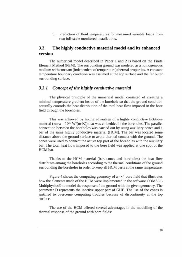
38
5. Prediction of fluid temperatures for measured variable loads from
two full-scale monitored installations.
3.3 The highly conductive material model and its enhanced
version
The numerical model described in Paper 1 and 2 is based on the Finite
Element Method (FEM). The surrounding ground was modeled as a homogeneous
medium with constant (independent of temperature) thermal properties. A constant
temperature boundary condition was assumed at the top surface and the far outer
surrounding surface.
3.3.1 Concept of the highly conductive material
The physical principle of the numerical model consisted of creating a
minimal temperature gradient inside of the borehole so that the ground condition
naturally controls the heat distribution of the total heat flow imposed in the bore
field through the boreholes.
This was achieved by taking advantage of a highly conductive fictitious
material (kHCM = 1010 W/(m-K)) that was embedded in the boreholes. The parallel
connection between the boreholes was carried out by using auxiliary cones and a
bar of the same highly conductive material (HCM). The bar was located some
distance above the ground surface to avoid thermal contact with the ground. The
cones were used to connect the active top part of the boreholes with the auxiliary
bar. The total heat flow imposed to the bore field was applied at one spot of the
HCM bar.
Thanks to the HCM material (bar, cones and boreholes) the heat flow
distributes among the boreholes according to the thermal conditions of the ground
surrounding the boreholes in order to keep all HCM parts at the same temperature.
Figure 4 shows the computing geometry of a 4×4 bore field that illustrates
how the elements made of the HCM were implemented in the software COMSOL
Multiphysics to model the response of the ground with the given geometry. The
parameter D represents the inactive upper part of GHE. The use of the cones is
justified to overcome computing troubles because of discontinuity at the top
surface.
The use of the HCM offered several advantages in the modelling of the
thermal response of the ground with bore fields:
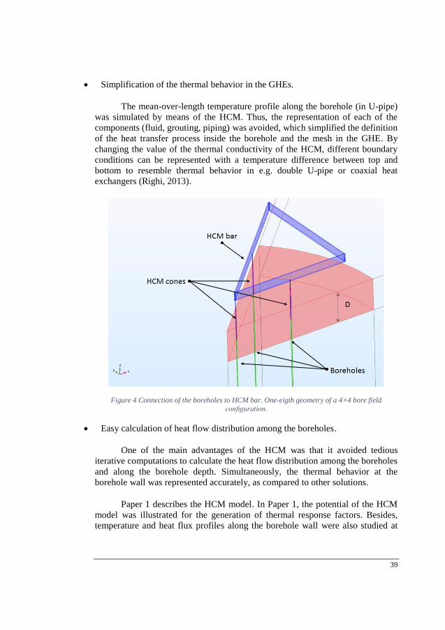
39
Simplification of the thermal behavior in the GHEs.
The mean-over-length temperature profile along the borehole (in U-pipe)
was simulated by means of the HCM. Thus, the representation of each of the
components (fluid, grouting, piping) was avoided, which simplified the definition
of the heat transfer process inside the borehole and the mesh in the GHE. By
changing the value of the thermal conductivity of the HCM, different boundary
conditions can be represented with a temperature difference between top and
bottom to resemble thermal behavior in e.g. double U-pipe or coaxial heat
exchangers (Righi, 2013).
Figure 4 Connection of the boreholes to HCM bar. One-eigth geometry of a 4×4 bore field
configuration.
Easy calculation of heat flow distribution among the boreholes.
One of the main advantages of the HCM was that it avoided tedious
iterative computations to calculate the heat flow distribution among the boreholes
and along the borehole depth. Simultaneously, the thermal behavior at the
borehole wall was represented accurately, as compared to other solutions.
Paper 1 describes the HCM model. In Paper 1, the potential of the HCM
model was illustrated for the generation of thermal response factors. Besides,
temperature and heat flux profiles along the borehole wall were also studied at
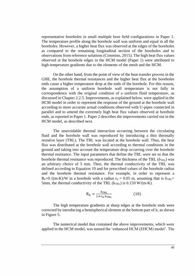
40
representative boreholes in small multiple bore field configurations in Paper 1.
The temperature profile along the borehole wall was uniform and equal in all the
boreholes. However, a higher heat flux was observed at the edges of the boreholes
as compared to the remaining longitudinal section of the boreholes and to
observations from reference solutions (Cimmino, 2015). The high heat flux values
observed at the borehole edges in the HCM model (Paper 1) were attributed to
high temperature gradients due to the elements of the mesh and the HCM.
On the other hand, from the point of view of the heat transfer process in the
GHE, the borehole thermal resistances and the higher heat flux at the boreholes
ends cause a higher temperature drop at the ends of the borehole. For this reason,
the assumption of a uniform borehole wall temperature is not fully in
correspondence with the original condition of a uniform fluid temperature, as
discussed in Chapter 2.2.5. Improvements, as explained below, were applied in the
HCM model in order to represent the response of the ground at the borehole wall
according to more accurate actual conditions observed with U-pipes connected in
parallel and to amend the extremely high heat flux values observed at borehole
ends, as reported in Paper 1. Paper 2 describes the improvements carried out in the
HCM model, as described next.
The unavoidable thermal interaction occurring between the circulating
fluid and the borehole wall was reproduced by introducing a thin thermally
resistive layer (TRL). The TRL was located at the borehole wall. Thus, the heat
flux was distributed at the borehole wall according to thermal conditions in the
ground and taking into account the temperature drop occurring over the borehole
thermal resistance. The input parameters that define the TRL were set so that the
borehole thermal resistance was reproduced. The thickness of the TRL (TRL) was
an arbitrary choice of 5 mm. Then, the thermal conductivity of the TRL was
defined according to Equation 10 and for prescribed values of the borehole radius
and the borehole thermal resistance. For example, in order to represent a
Rb=0.1(m-K)/W in a borehole with a radius rb = 0.05 m, assuming that is TRL=
5mm, the thermal conductivity of the TRL (kTRL) is 0.159 W/(m-K).
Rb =δTRL
2∙π∙rb∙kTRL (10)
The high temperature gradients at sharp edges at the borehole ends were
corrected by introducing a hemispherical element at the bottom part of it, as shown
in Figure 5.
The numerical model that contained the above improvements, which were
applied in the HCM model, was named the ‘enhanced HCM (EHCM) model’. The
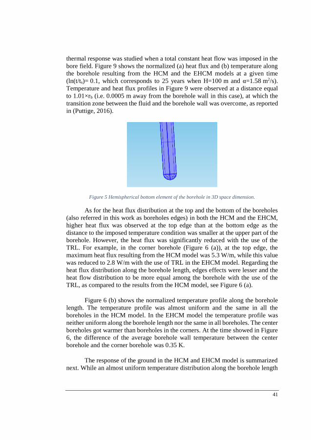
41
thermal response was studied when a total constant heat flow was imposed in the
bore field. Figure 9 shows the normalized (a) heat flux and (b) temperature along
the borehole resulting from the HCM and the EHCM models at a given time
(ln(t/ts)= 0.1, which corresponds to 25 years when H=100 m and α=1.58 m2/s).
Temperature and heat flux profiles in Figure 9 were observed at a distance equal
to 1.01×rb (i.e. 0.0005 m away from the borehole wall in this case), at which the
transition zone between the fluid and the borehole wall was overcome, as reported
in (Puttige, 2016).
Figure 5 Hemispherical bottom element of the borehole in 3D space dimension.
As for the heat flux distribution at the top and the bottom of the boreholes
(also referred in this work as boreholes edges) in both the HCM and the EHCM,
higher heat flux was observed at the top edge than at the bottom edge as the
distance to the imposed temperature condition was smaller at the upper part of the
borehole. However, the heat flux was significantly reduced with the use of the
TRL. For example, in the corner borehole (Figure 6 (a)), at the top edge, the
maximum heat flux resulting from the HCM model was 5.3 W/m, while this value
was reduced to 2.8 W/m with the use of TRL in the EHCM model. Regarding the
heat flux distribution along the borehole length, edges effects were lesser and the
heat flow distribution to be more equal among the borehole with the use of the
TRL, as compared to the results from the HCM model, see Figure 6 (a).
Figure 6 (b) shows the normalized temperature profile along the borehole
length. The temperature profile was almost uniform and the same in all the
boreholes in the HCM model. In the EHCM model the temperature profile was
neither uniform along the borehole length nor the same in all boreholes. The center
boreholes got warmer than boreholes in the corners. At the time showed in Figure
6, the difference of the average borehole wall temperature between the center
borehole and the corner borehole was 0.35 K.
The response of the ground in the HCM and EHCM model is summarized
next. While an almost uniform temperature distribution along the borehole length
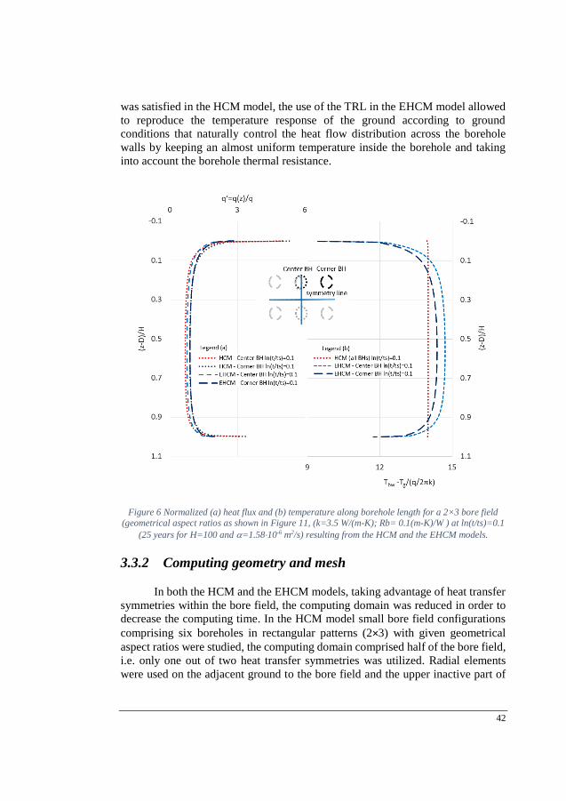
42
was satisfied in the HCM model, the use of the TRL in the EHCM model allowed
to reproduce the temperature response of the ground according to ground
conditions that naturally control the heat flow distribution across the borehole
walls by keeping an almost uniform temperature inside the borehole and taking
into account the borehole thermal resistance.
Figure 6 Normalized (a) heat flux and (b) temperature along borehole length for a 2×3 bore field (geometrical aspect ratios as shown in Figure 11, (k=3.5 W/(m-K); Rb= 0.1(m-K)/W ) at ln(t/ts)=0.1
(25 years for H=100 and =1.5810-6 m2/s) resulting from the HCM and the EHCM models.
3.3.2 Computing geometry and mesh
In both the HCM and the EHCM models, taking advantage of heat transfer
symmetries within the bore field, the computing domain was reduced in order to
decrease the computing time. In the HCM model small bore field configurations
comprising six boreholes in rectangular patterns (2×3) with given geometrical
aspect ratios were studied, the computing domain comprised half of the bore field,
i.e. only one out of two heat transfer symmetries was utilized. Radial elements
were used on the adjacent ground to the bore field and the upper inactive part of
43
the bore field. Therefore, radial elements resulted from a triangular mesh drawn
on the layer above the active depth of the bore field, with small elements in the
bore field region which increased as the distance moved further away from the
bore field. Then, the triangular elements were swept along the borehole depth with
a symmetric distribution and smaller elements near the borehole edges. The
triangular elements were also swept along the region above the active part of the
bore field. The mesh of the region downward the bore field was made up of
tetrahedral elements, with small elements in the bore field region that increased
their size as mesh moving further the bore field region. The total number of
elements in the mesh in the HCM model was around 250,000.
In the EHCM model, the mesh was similar to the HCM model, but
including some improvements that increased the accuracy and continued to
provide the solution within an acceptable time (8 hours for the generation of
temperature response with a continuous heat flow and less than 1% of total heat
flow (post)calculations). These improvements included the reduction of the
computing geometries to the greatest extent, i.e. computing domains of rectangular
2×3 and 4×4 bore fields were reduced to one-quarter and one-eighth, respectively.
Figure 7 shows the computing domain of a 4×4 bore field. The elements of
the mesh in the bore field region and the nearest surrounding (one-eighth cylinder
with an outer radius of 20 m) also consisted of radial elements built from a swept
operation of the triangular elements, see Figure 7 – ‘zoom 1’, of the surface above
the active upper part and along the bore field length. Tetrahedral elements
comprised the surrounding outward of the bore field region. The region downward
of the bore field and the elements made up of the HCM were also meshed with
tetrahedral elements. Elements of the mesh in the bore field region and nearest
bore field surrounding are shown in Figure 7 – ‘zoom 2’ to illustrate the meshing
process. The mesh in the EHCM model consisted of 200,000 elements in total.
The simulation of both the HCM and EHCM models were carried out on a
computer with 32 GB RAM and two Intel© Xeon© processors CPU E5-2620 at
2.00 GHz.
3.4 Results
The HCM and EHCM models were utilized to simulate the response of the
ground with a continuous total heat flow imposed to the bore field for the
generation of temperature response functions.
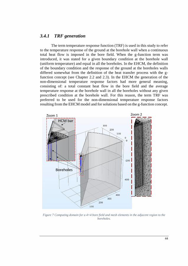
44
3.4.1 TRF generation
The term temperature response function (TRF) is used in this study to refer
to the temperature response of the ground at the borehole wall when a continuous
total heat flow is imposed in the bore field. When the g-function term was
introduced, it was stated for a given boundary condition at the borehole wall
(uniform temperature) and equal in all the boreholes. In the EHCM, the definition
of the boundary condition and the response of the ground at the boreholes walls
differed somewhat from the definition of the heat transfer process with the g-
function concept (see Chapter 2.2 and 2.3). In the EHCM the generation of the
non-dimensional temperature response factors had more general meaning,
consisting of: a total constant heat flow in the bore field and the average
temperature response at the borehole wall in all the boreholes without any given
prescribed condition at the borehole wall. For this reason, the term TRF was
preferred to be used for the non-dimensional temperature response factors
resulting from the EHCM model and for solutions based on the g-function concept.
Figure 7 Computing domain for a 4×4 bore field and mesh elements in the adjacent region to the
boreholes.
45
Firstly, the HCM model was utilized to generate the TRFs for the single
borehole and small multiple bore field configurations of two 2×3 bore fields, as
reported in Paper 1. Then, the EHCM model was utilized to obtain the TRFs of
the same small bore fields reported in Paper 1 and expanded to a larger 4×4 bore
field configuration, as shown in Paper 2. In the EHCM model, the GHE thermal
resistance is assumed to be Rb = 0.1 (m-K)/W and the soil thermal conductivity,
k= 3.5 W/(m-K).
Figure 8 shows the TRF of a 4×4 bore field with given geometrical aspect
ratios obtained from the HCM and the EHCM model, tagged as “FEM - HCM”
and “FEM - EHCM”, respectively. Besides, the TRFs from reference solutions are
also illustrated in Figure 8. The reference solution tagged as “FDM – Uniform
Temperature” is based on the SBM approach with uniform temperature and
obtained from commercial design tools (Hellström and Sanner, 1994). The
solution obtained from the FLS with uniform temperature is tagged as “FLS –
Uniform Temperature”. Figure 8 also includes the TRF resulting from a recent
state-of-the-art approach proposed in (Cimmino, 2015b) with a non-dimensional
thermal conductance of 0.300, a non-dimensional fluid flow rate 0.9425 and a non-
dimensional borehole thermal resistance of 2.19 with k= 3.5 W/(m-K). This
solution is tagged as Cimmino 2015. The TRFs are expressed as a function of
ln(t/ts).
In general, at short times, differences between the solutions were small. At
ln(t/ts)=-4.5 (around 200 days for H=150 and α=1.5810-6 m2/s), the TRF from the
HCM model underestimated the response by 0.03 units as compared to the
response from the EHCM model. At ln(t/ts)=-4.5, the solution from the ‘FLS –
Uniform Temperature’ also underestimated the response by 0.01 units as
compared to EHCM predictions and resulted in higher predictions than those from
the HCM model, by around 0.05 units. The TRF- ‘FDM – Uniform Temperature’
was around 0.1 units higher than the TRF- ‘FEM - EHCM’ when ln(t/ts)=-4.5. A
difference of 0.1 units in the TRFs represents a 0.09 K in terms of temperature
when a constant heat rate per unit length of 20 W/m is assumed, and the thermal
conductivity of the soil is 3.5 W/(m-K).
The differences increased with time, being noticeable when ln(t/ts)> 0
(around 50 years for H=150 and α=1.5810-6 m2/s). For instance, when ln(t/ts)=
1.5, the TRF- “FEM - HCM” underestimated the response by 0.9 units (3.4%) as
compared to the TRF- “FEM – EHCM”. A similar behavior was observed when
the TRF- “FLS – Uniform Temperature” was compared to the TRF- “FEM –
EHCM” with an under prediction of around 0.5 units (2%). As time increases, the
TRF – “FDM – Uniform Temperature” tended to overestimate the response, being
around 0.5 units (2%) at ln(t/ts)= 1.5. In terms of temperature differences, a 0.5
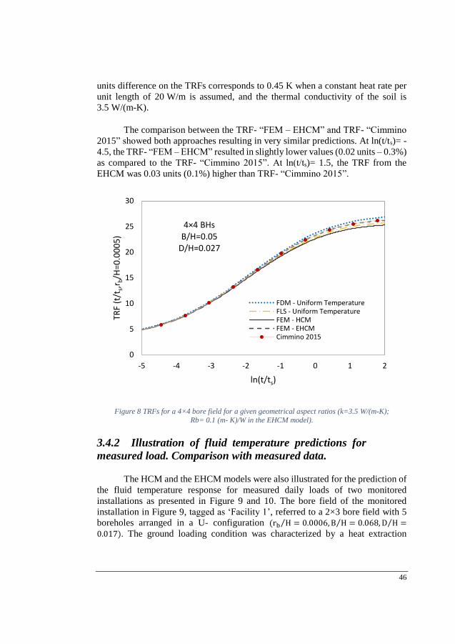
46
units difference on the TRFs corresponds to 0.45 K when a constant heat rate per
unit length of 20 W/m is assumed, and the thermal conductivity of the soil is
3.5 W/(m-K).
The comparison between the TRF- “FEM – EHCM” and TRF- “Cimmino
2015” showed both approaches resulting in very similar predictions. At ln(t/ts)= -
4.5, the TRF- “FEM – EHCM” resulted in slightly lower values (0.02 units – 0.3%)
as compared to the TRF- “Cimmino 2015”. At ln(t/ts)= 1.5, the TRF from the
EHCM was 0.03 units (0.1%) higher than TRF- “Cimmino 2015”.
Figure 8 TRFs for a 4×4 bore field for a given geometrical aspect ratios (k=3.5 W/(m-K);
Rb= 0.1 (m- K)/W in the EHCM model).
3.4.2 Illustration of fluid temperature predictions for
measured load. Comparison with measured data.
The HCM and the EHCM models were also illustrated for the prediction of
the fluid temperature response for measured daily loads of two monitored
installations as presented in Figure 9 and 10. The bore field of the monitored
installation in Figure 9, tagged as ‘Facility 1’, referred to a 2×3 bore field with 5
boreholes arranged in a U- configuration (rb H⁄ = 0.0006, B H⁄ = 0.068, D H⁄ =
0.017). The ground loading condition was characterized by a heat extraction
0
5
10
15
20
25
30
-5 -4 -3 -2 -1 0 1 2
TRF
(t/t
s,r b
/H=0
.00
05
)
ln(t/ts)
4×4 BHsB/H=0.05
D/H=0.027
FDM - Uniform TemperatureFLS - Uniform TemperatureFEM - HCMFEM - EHCMCimmino 2015
47
profile in order to supply space heating in the winter season and domestic hot water
over the entire year. The total annual energy imbalance was of around 40 MWh.
‘Facility 1’ was monitored since February 2010 till December 2013 when the
monitoring system stopped being functional. Further information about ‘Facility
1’ was reported in (Iglesias et al., 2012 and Puttige et al., 2016).
The bore field corresponding to the second monitored installation analyzed
in this dissertation was referred to ‘Facility 2’. Its measured data is presented in
Figure 10. The bore field consisted of a rectangular 2×3 bore field with the
following geometrical aspect ratios (rb H⁄ = 0.0016, B H⁄ = 0.063, D H⁄ = 0.074). The GCHP system supplied space heating during the winter and space cooling
during the summer. The total annual thermal imbalance was around 24.7 MWh of
cooling load. ‘Facility 2’ has been monitored since the beginning of its operation
in January 2005 up to now. The comparison of fluid temperature prediction against
measured data presented in this dissertation was done until June 2015. More
details about Facility 2 can be found in (Montagud et al., 2011; GroundMed, 2014
and Ruiz-Calvo et al., 2016).
The computing geometries of the monitored bore fields were first built
according to their geometrical aspect ratios. The thermal properties of the ground
and its undisturbed temperature in the models were defined according to
predictions from TRTs. A detailed description of the monitored installations and
a summary of the data source of the monitored installations can be found in
Paper 2.
Then, both the HCM and EHCM models were first used to generate their
TRFs, as shown in Paper 2. Next, in the HCM and the EHCM models, the
continuous total heat flow value was replaced by the measured thermal power
exchanged with the ground at monitored sites. Thus, the ground response was
predicted from both the HCM and EHCM models for the corresponding measured
bore field loads. Then, the average fluid temperature (Tf) was obtained from the
relation between the average temperature at the borehole wall (Tb) and to the heat
transfer rate per unit length (q) affected by the traditional effective GHE thermal
resistance (Rb∗), with t defined as daily steps, as expressed in Equation 1.
Figure 9 and 10 show the comparison of the fluid temperature predictions
against measured values for Facility 1 and Facility 2, respectively. The accuracy
of both the EHCM and the HCM models to predict daily temperature was
examined from the deviation of the ‘Simulated Daily Temp FEM-EHCM’ against
‘Measured Daily Temp’ for both ‘Facility 1’ and ‘Facility 2’. The analysis was
also carried out for predictions obtained from a FEM with constant heat flux
boundary condition at the borehole wall.
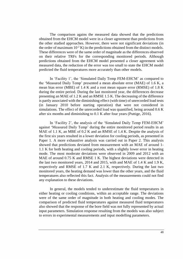
48
The comparison agains the measured data showed that the predictions
obtained from the EHCM model were in a closer agreement than predictions from
the other studied approaches. However, there were not significant deviations (in
the order of maximum 10-2 K) in the predictions obtained from the distinct models.
These differences were of the same order of magnitude as the differences observed
on their relative TRFs for the corresponding monitored periods. Although
predictions obtained from the EHCM model presented a closer agreement with
measured data, the reduction of the error was too small to state the EHCM model
predicted the fluid temperatures more accurately than other models.
In ‘Facility 1’, the ‘Simulated Daily Temp FEM-EHCM’ as compared to
the ‘Measured Daily Temp’ presented a mean absolute error (MAE) of 1.6 K, a
mean bias error (MBE) of 1.4 K and a root mean square error (RMSE) of 1.8 K
during the entire period. During the last monitored year, the differences decrease
presenting an MAE of 1.2 K and an RMSE 1.5 K. The decreasing of the difference
is partly associated with the diminishing effect (with time) of unrecorded load tests
(in January 2010 before starting operation) that were not considered in
simulations. The effect of the unrecorded load was quantified, being around 0.6 K
after six months and diminishing to 0.1 K after four years (Puttige, 2016).
In ‘Facility 2’, the analysis of the ‘Simulated Daily Temp FEM-EHCM’
against ‘Measured Daily Temp’ during the entire monitored period results in an
MAE of 1.1 K, an MBE of 0.2 K and an RMSE of 1.4 K. Despite the analysis of
the first six years resulted in a lower deviation for cooling periods, as presented in
Paper 1. A more exhaustive analysis was carried out in Paper 2. This analysis
showed that predictions deviated from measurement with an MAE of around 1-
1.1 K for both heating and cooling periods, with a slightly lower error in heating
mode. The most moderate deviations were observed in 2009 and 2012 with an
MAE of around 0.75 K and RMSE 1 K. The highest deviations were detected in
the last two monitored years, 2014 and 2015, with and MAE of 1.4 K and 1.9 K,
respectively and RMSE of 1.7 K and 2.1 K, respectively. During the last two
monitored years, the heating demand was lower than the other years, and the fluid
temperatures also reflected this fact. Analysis of the measurements could not find
any explanation to these deviations.
In general, the models tended to underestimate the fluid temperatures in
either heating or cooling conditions, within an acceptable range. The deviations
were of the same order of magnitude in both heating and cooling modes. The
comparison of predicted fluid temperatures against measured fluid temperatures
also showed that the response of the bore field was not fully represented by actual
input parameters. Simulation response resulting from the models was also subject
to errors in experimental measurements and input modelling parameters.
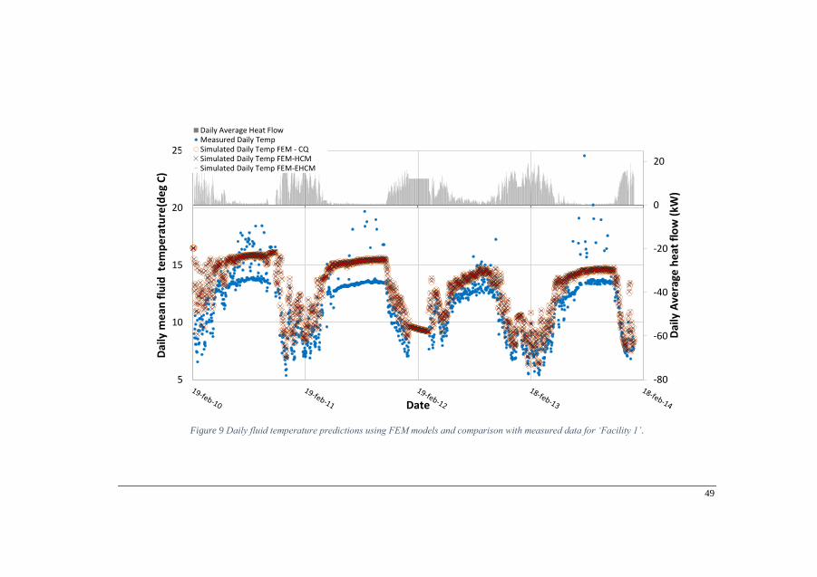
49
Figure 9 Daily fluid temperature predictions using FEM models and comparison with measured data for ‘Facility 1’.
-80
-60
-40
-20
0
20
5
10
15
20
25
Dai
ly A
vera
ge h
eat
flo
w (
kW)
Dai
ly m
ean
flu
id t
em
pe
ratu
re(d
eg
C)
Date
Daily Average Heat FlowMeasured Daily TempSimulated Daily Temp FEM - CQSimulated Daily Temp FEM-HCMSimulated Daily Temp FEM-EHCM
50
Figure 10 Daily fluid temperature predictions using FEM models and comparison with measured data for ‘Facility 2.
-30
-25
-20
-15
-10
-5
0
5
10
10
15
20
25
30
35
40
45
Dai
ly A
vera
ge H
eat
Flo
w (
kW)
Dai
ly f
luid
te
mp
era
ture
(d
egC
)
Date
Daily Average Heat FlowMeasured Daily TempSimulated Daily Temp FEM - CQSimulated Daily Temp FEM - HCMSimulated Daily Temp FEM - EHCM
51
3.5 Conclusions
A numerical model was developed for the response of the ground in bore
field with the GHE connected in parallel. The developed model did not impose
any boundary condition at the borehole wall, as it is often done in reference
studies. In the developed model the boundary condition was defined as a total heat
flow. The ground conditions naturally control the heat flux distribution at the wall
of the borehole.
For this purpose, boreholes were filled with a fictitious highly conductive
material. Then, an auxiliary bar of the same highly conductive material, located
somewhat above the top surface, was connected to the boreholes. The purpose of
the bar was to emulate the parallel connection among the boreholes. The inactive
upper part above the active borehole length of the borehole was represented via an
auxiliary cone that connected the top active part of the borehole to the bar. The
total heat flow was imposed at one spot in the auxiliary bar. The thermal
conductivity of the material was so high that the temperature gradient occurring
within the highly conductive material was very small. Therefore, the ground
condition was naturally establishing the heat transfer through the walls of the
boreholes. This model was used to study the temperature and heat flux distribution
along the borehole length in some bore field configurations.
Moreover, the definition of the boundary condition was also subject of
discussion in this work. As discussed, the assumption of a uniform borehole wall
temperature is violated when it is considered that the thermal resistance between
the borehole wall and the circulating fluid and the heat flux variations interact
along the borehole. This aspect has often been disregarded. Improvements were
applied in the enhanced version of the proposed model in order to take into account
this aspect. This was achieved by introducing a thermal resistive layer at the
borehole wall. Moreover, edge effects at the borehole ends were also softened by
representing the borehole bottom as a hemispherical element. This enhanced
model was also used to study the temperature and heat flux profiles at the borehole
wall. The effect of the thermal resistance between the circulating fluid and the
borehole wall were proved to violate the assumption of a uniform temperature at
the borehole wall, which also distorted the heat flow distribution between the
boreholes.
The thermal response functions (with continuous and constant total heat
flow in the bore field) were generated from the proposed model and its enhanced
version. TRFs resulting from the enhanced version of the numerical model serve
as reference to other solutions. The numerical model and its enhanced version were
also tested to predict the fluid temperature for the multiyear operation of two

52
monitored installations. Although predictions from the enhanced model presented
a closer agreement with measured data than predictions resulting from other
models, differences were not significant enough to state that the enhanced model
predicted the response of the bore field more accurately. The analysis of the
deviations showed that the models tended to underestimate the response of the
bore field and did not fully represent the response of the bore field for actual input
parameters. The enhanced model predicted fluid temperatures with a mean
absolute error varying within 1.1 K and 1.6 K and a root mean square root within
1.4 K and 1.8 K, which was an acceptable variation that should not compromise
the performance of the heat pump.

53
4 BORE FIELD SIZING: INFLUENCE OF DESIGN
PARAMETERS
Mathematical models are used in bore field sizing methods to predict the return fluid
temperature. Besides the mathematical approach, bore field sizing methods are used to
calculate the required length in order to keep the return fluid temperature within certain
limits at the worst ground load condition. The worst ground load condition is usually
assumed to occur after 10 or 20 years. However, the worst ground load condition often occurs
during the first year of operation. A general methodology that allows the calculation of the
required bore field length during the first year of operation and at any longer time was
proposed in Paper 3. A comprehensive summary of the proposed methodology is described
in this Chapter 4. The potential of the methodology was illustrated for a particular case
with a quasi-balanced annual load condition with application to optimum borehole spacing.
4.1 Specific objective
The specific objective of Chapter 4 was to develop a general bore field
sizing methodology. This methodology should be able to:
(i) Evaluate the total bore field length for the first year of operation and
at any longer times of operation
(ii) Study the optimum borehole spacing for quasi-balanced load
scenarios
4.2 Method
1. Revision of reference studies, as summarized in Chapter 2.3.2.
2. Development of a general bore field sizing methodology
3. Application of the methodology to calculate the bore field length for
the first year of operation and after 10 years of operation. The
methodology is also applied to find the optimum borehole spacing
for a quasi-balanced load scenario. Discussion of the results.
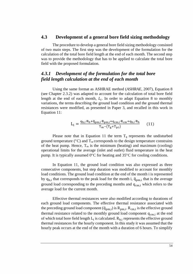
54
4.3 Development of a general bore field sizing methodology
The procedure to develop a general bore field sizing methodology consisted
of two main steps. The first step was the development of the formulation for the
calculation of the total bore field length at the end of each month. The second step
was to provide the methodology that has to be applied to calculate the total bore
field with the proposed formulation.
4.3.1 Development of the formulation for the total bore
field length calculation at the end of each month
Using the same format as ASHRAE method (ASHRAE, 2007), Equation 8
(see Chapter 2.3.2) was adapted to account for the calculation of total bore field
length at the end of each month, 𝐿𝑖. In order to adapt Equation 8 to monthly
variations, the terms describing the ground load condition and the ground thermal
resistances were modified, as presented in Paper 3, and recalled in this work in
Equation 11:
Li =qh,i∙Rb+qpm,i∙Rpm,i+qcm,i∙Rcm+qh,i∙Rh
Tm−(Tg+Tp,i) (11)
Please note that in Equation 11 the term Tg represents the undisturbed
ground temperature (C) and Tm corresponds to the design temperature constrains
of the heat pump. Hence, Tm is the minimum (heating) and maximum (cooling)
operational limits for the average (inlet and outlet) fluid temperature in the heat
pump. It is typically assumed 0C for heating and 35C for cooling conditions.
In Equation 11, the ground load condition was also expressed as three
consecutive components, but step duration was modified to account for monthly
load conditions. The ground load condition at the end of the month i is represented
by qh,i that corresponds to the peak load for the month i, qpm,i that is the average
ground load corresponding to the preceding months and qcm,i which refers to the
average load for the current month.
Effective thermal resistances were also modified according to durations of
each ground load components. The effective thermal resistance associated with
the preceding ground load component (qpm,i) is Rpm,i. Rcm,i is the effective ground
thermal resistance related to the monthly ground load component qcm,i at the end
of which total bore field length Li is calculated. Rh,i represents the effective ground
thermal resistances for the hourly component. In this study it was assumed that the
hourly peak occurs at the end of the month with a duration of 6 hours. To simplify
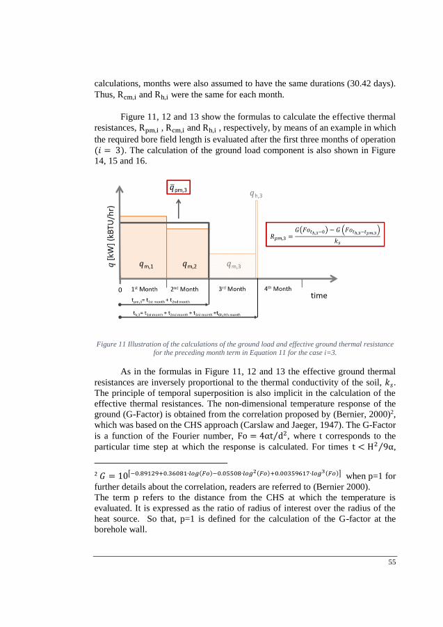
55
calculations, months were also assumed to have the same durations (30.42 days).
Thus, Rcm,i and Rh,i were the same for each month.
Figure 11, 12 and 13 show the formulas to calculate the effective thermal
resistances, Rpm,i , Rcm,i and Rh,i , respectively, by means of an example in which
the required bore field length is evaluated after the first three months of operation
(𝑖 = 3). The calculation of the ground load component is also shown in Figure
14, 15 and 16.
Figure 11 Illustration of the calculations of the ground load and effective ground thermal resistance for the preceding month term in Equation 11 for the case i=3.
As in the formulas in Figure 11, 12 and 13 the effective ground thermal
resistances are inversely proportional to the thermal conductivity of the soil, 𝑘𝑠.
The principle of temporal superposition is also implicit in the calculation of the
effective thermal resistances. The non-dimensional temperature response of the
ground (G-Factor) is obtained from the correlation proposed by (Bernier, 2000)2,
which was based on the CHS approach (Carslaw and Jaeger, 1947). The G-Factor
is a function of the Fourier number, Fo = 4αt d2⁄ , where t corresponds to the
particular time step at which the response is calculated. For times t < H2 9α⁄ ,
2 𝐺 = 10[−0.89129+0.36081∙𝑙𝑜𝑔(𝐹𝑜)−0.05508∙𝑙𝑜𝑔2(𝐹𝑜)+0.00359617∙𝑙𝑜𝑔3(𝐹𝑜)] when p=1 for
further details about the correlation, readers are referred to (Bernier 2000).
The term p refers to the distance from the CHS at which the temperature is
evaluated. It is expressed as the ratio of radius of interest over the radius of the
heat source. So that, p=1 is defined for the calculation of the G-factor at the
borehole wall.
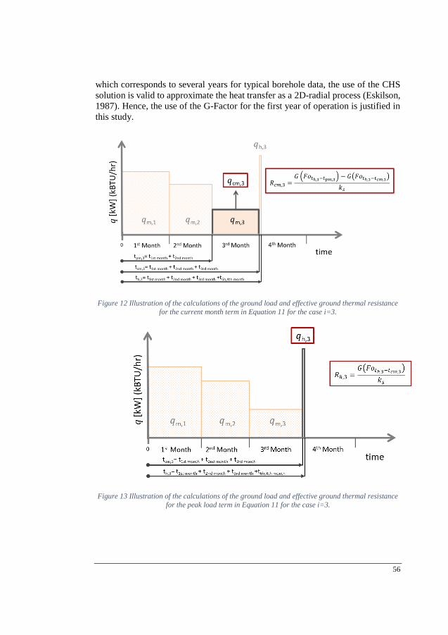
56
which corresponds to several years for typical borehole data, the use of the CHS
solution is valid to approximate the heat transfer as a 2D-radial process (Eskilson,
1987). Hence, the use of the G-Factor for the first year of operation is justified in
this study.
Figure 12 Illustration of the calculations of the ground load and effective ground thermal resistance
for the current month term in Equation 11 for the case i=3.
Figure 13 Illustration of the calculations of the ground load and effective ground thermal resistance
for the peak load term in Equation 11 for the case i=3.
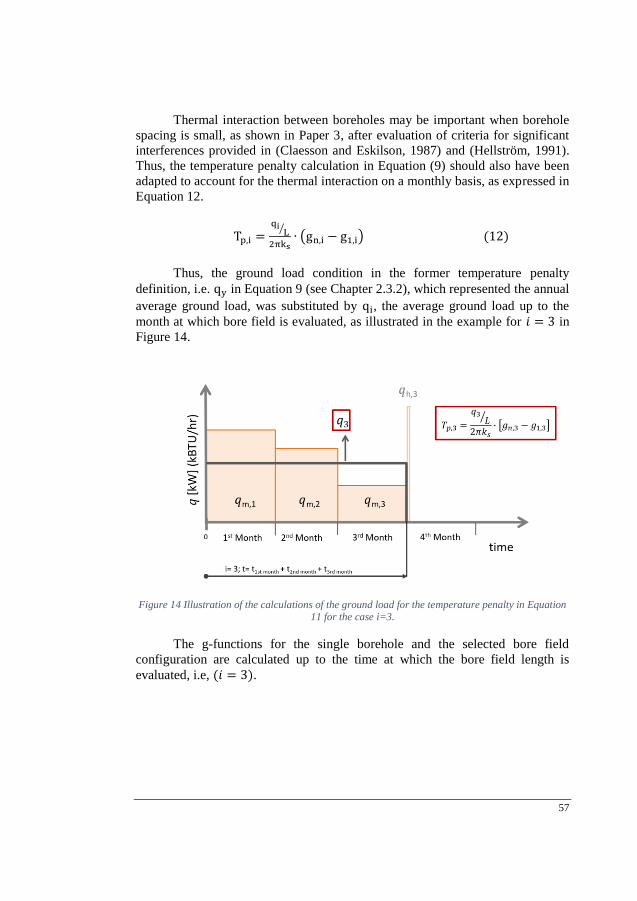
57
Thermal interaction between boreholes may be important when borehole
spacing is small, as shown in Paper 3, after evaluation of criteria for significant
interferences provided in (Claesson and Eskilson, 1987) and (Hellström, 1991).
Thus, the temperature penalty calculation in Equation (9) should also have been
adapted to account for the thermal interaction on a monthly basis, as expressed in
Equation 12.
Tp,i =qi
L⁄
2πks∙ (gn,i − g1,i) (12)
Thus, the ground load condition in the former temperature penalty
definition, i.e. qy in Equation 9 (see Chapter 2.3.2), which represented the annual
average ground load, was substituted by qi, the average ground load up to the
month at which bore field is evaluated, as illustrated in the example for 𝑖 = 3 in
Figure 14.
Figure 14 Illustration of the calculations of the ground load for the temperature penalty in Equation 11 for the case i=3.
The g-functions for the single borehole and the selected bore field
configuration are calculated up to the time at which the bore field length is
evaluated, i.e, (𝑖 = 3).
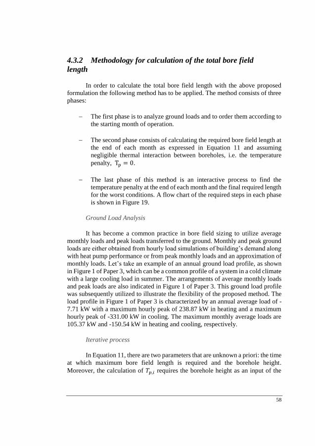
58
4.3.2 Methodology for calculation of the total bore field
length
In order to calculate the total bore field length with the above proposed
formulation the following method has to be applied. The method consists of three
phases:
The first phase is to analyze ground loads and to order them according to
the starting month of operation.
The second phase consists of calculating the required bore field length at
the end of each month as expressed in Equation 11 and assuming
negligible thermal interaction between boreholes, i.e. the temperature
penalty, Tp = 0.
The last phase of this method is an interactive process to find the
temperature penalty at the end of each month and the final required length
for the worst conditions. A flow chart of the required steps in each phase
is shown in Figure 19.
Ground Load Analysis
It has become a common practice in bore field sizing to utilize average
monthly loads and peak loads transferred to the ground. Monthly and peak ground
loads are either obtained from hourly load simulations of building’s demand along
with heat pump performance or from peak monthly loads and an approximation of
monthly loads. Let’s take an example of an annual ground load profile, as shown
in Figure 1 of Paper 3, which can be a common profile of a system in a cold climate
with a large cooling load in summer. The arrangements of average monthly loads
and peak loads are also indicated in Figure 1 of Paper 3. This ground load profile
was subsequently utilized to illustrate the flexibility of the proposed method. The
load profile in Figure 1 of Paper 3 is characterized by an annual average load of -
7.71 kW with a maximum hourly peak of 238.87 kW in heating and a maximum
hourly peak of -331.00 kW in cooling. The maximum monthly average loads are
105.37 kW and -150.54 kW in heating and cooling, respectively.
Iterative process
In Equation 11, there are two parameters that are unknown a priori: the time
at which maximum bore field length is required and the borehole height.
Moreover, the calculation of 𝑇𝑝,𝑖 requires the borehole height as an input of the
59
geometrical aspect ratios of the bore field layout for the g-function calculation.
Therefore, an iterative procedure is required to solve Equation 11. For given input
parameters as listed in the first step of the flow chart in Figure 16, the calculation
procedure starts with the analysis of the ground load and the calculation of the
effective ground thermal resistances.
Figure 15 Flowchart containing the steps of the iterative process to calculate L in Equation 11
(presented in Paper 3).
60
Then, in the first iteration, Tp,i is assumed to be zero. A set of required total
bore field lengths is obtained for heating and cooling conditions at the end of each
month, LiH and Li
C, respectively. Among the 24 values of L, the maximum value
is chosen to be used in the next calculations, identified as LNEW in Figure 16. In
the next steps temperature penalties are calculated. The g-function requires the
borehole height which is estimated from 𝐿𝑁𝐸𝑊 and a prescribed number of
boreholes, nb as H =LNEW
nb. Once borehole height is estimated, the geometrical
aspect ratios are given as input for the calculation of the g-function values via an
interpolation procedure of a pre calculated g-function for a given bore field
geometry.
Applying Equation 12, a set of temperature penalties is obtained for each
month and for a given ratio B
H in heating and cooling conditions, Tp,i
H and Tp,iC ,
respectively. Then, calculation of L is again carried out for the temperature
penalties at each month. This procedure is repeated until a convergence criterion
is met (1%). It is worth noticing that this methodology is adjustable for multi-year
simulation.
4.4 Application of the methodology
4.4.1 Calculation of the required total bore field length
at the end of each month during the first year of operation
For a particular ground load profile with a quasi-balanced load condition,
see Figure 15 and prescribed input parameters listed in Table 5 –Paper 3, the
methodology was first applied to calculate the total bore field length at the end of
each month during the first year of operation. These results were provided in Table
6 of Paper 3. Two different starting dates of operation were also evaluated, January
1 and July 1. The analysis of these results showed that a 5% reduction of the total
required bore field length was achieved when the system was started in July. When
operation of the system started in July 1, the ground increased its temperature
during the heat injection period, which harnessed the system during the heat
extraction period. A sensitivity analysis of the starting dates during the first year
of operation was carried out in Appendix B of Paper 3, with a minimum required
𝐿 when system started in May, 1.
Calculation of the total required bore field length after ten years of
operation, i.e. using the traditional ASHRAE method (Equation 8), resulted in
4921 m for the particular case considered in this study. If a 10-year period had
only been considered for bore field sizing, without looking into the response
61
during the first year of operation, the bore field would have been undersized for
the conditions during the first year, which could have caused operational problems
during this period.
It is worth to mention that systems with ground load conditions similar to
the example presented in this study (maximum length during the first year of
operation) may design (and drill) the bore field for typical time-span conditions
(10 years) and use a complementary heating system during the first year as an
alternative to prevent the system to run into operational problems and to install
more pipe than needed. This methodology (Paper 3) allows designer to calculate
the required total bore field length at any time-span and to take decision to
optimize the design without incurring in either operational problems or
unnecessary extra cost.
Thermal diffusivity of the ground was also an important aspect on the total
required bore field length. Paper 3 gathered an analysis of the results for the given
example in this study to illustrate how total bore field length was affected by a set
of given values of thermal ground diffusivity in combination with a set of two
given borehole spacings.
4.4.2 Optimum borehole spacing
Secondly, the methodology was also utilized to evaluate the reduction of
the borehole spacing on the total bore field length calculation. The analysis was
performed for two starting dates (January 1 and July 1) and during the first and the
tenth year of operation. The total bore field length was evaluated at the end of each
month for a set of borehole spacings that varied from 6 to 3 m in steps of 1 m.
Maximum required bore field length against borehole spacing for the two starting
dates are shown in Figure 17 for the first year of operation and in Figure 18 for the
tenth year of operation.
For the example considered in this study with starting date July 1, the total
required bore field could be minimized from 5853 m for a borehole spacing of 6
m down to 5620 m for a borehole spacing of 3 m (for the tenth year of operation).
By reducing the borehole spacing, the temperature in the bore field increases or
the heat losses to the surroundings decreases. The increase of temperature benefits
the system in heating operation during the upcoming winter season.
Therefore, results for the particular case with a quasi- balanced thermal
load considered in this study showed the capability of the proposed methodology
to handle this type of questions and that it was possible to find an optimum
borehole spacing that minimizes the total required bore field.
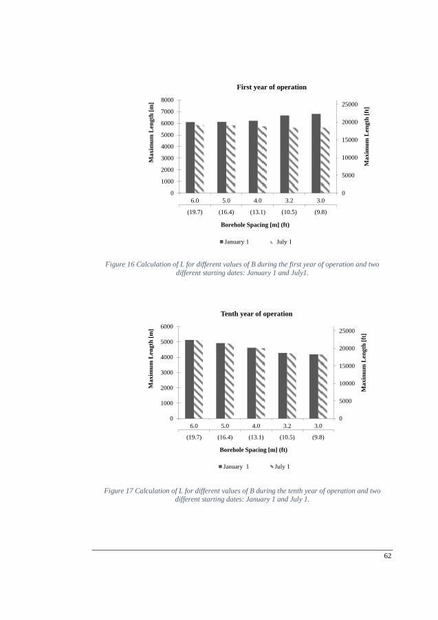
62
Figure 16 Calculation of L for different values of B during the first year of operation and two
different starting dates: January 1 and July1.
Figure 17 Calculation of L for different values of B during the tenth year of operation and two different starting dates: January 1 and July 1.
(19.7) (16.4) (13.1) (10.5) (9.8)
0
5000
10000
15000
20000
25000
0
1000
2000
3000
4000
5000
6000
7000
8000
6.0 5.0 4.0 3.2 3.0
Ma
xim
um
Len
gth
[ft
]
Ma
xim
um
Len
gth
[m
]
Borehole Spacing [m] (ft)
First year of operation
January 1 July 1
(19.7) (16.4) (13.1) (10.5) (9.8)
0
5000
10000
15000
20000
25000
0
1000
2000
3000
4000
5000
6000
6.0 5.0 4.0 3.2 3.0
Ma
xim
um
Len
gth
[ft
]
Ma
xim
um
Len
gth
[m
]
Borehole Spacing [m] (ft)
Tenth year of operation
January 1 July 1

63
4.5 Conclusions
A general methodology to calculate the required bore field length was
developed.
The proposed methodology calculates the total bore field length at the
end of each month during the first year of operation or at any longer
times.
The methodology also allows to find the optimum borehole spacing that
minimizes the total bore field length for quasi-balanced annual load
scenarios.
The proposed methodology was illustrated for a particular ground load
condition. The results showed that the maximum required length occurred during
the first year of operation which would have led the system to run into to
operational problems if a typical 10-year span period had been considered in the
calculations. The methodology was also applied to find the optimum borehole
spacing for a particular quasi-balanced load profile.
Sizing equation (Equation 8) in ASHRAE HandbookHVAC
Applications is recommended to be changed as proposed in Equation 11.

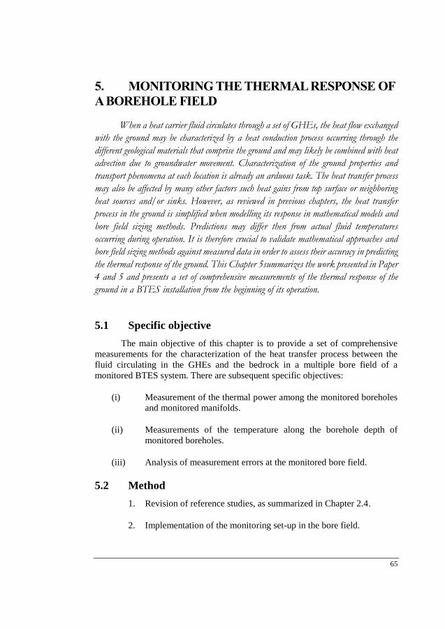
65
5. MONITORING THE THERMAL RESPONSE OF
A BOREHOLE FIELD
When a heat carrier fluid circulates through a set of GHEs, the heat flow exchanged
with the ground may be characterized by a heat conduction process occurring through the
different geological materials that comprise the ground and may likely be combined with heat
advection due to groundwater movement. Characterization of the ground properties and
transport phenomena at each location is already an arduous task. The heat transfer process
may also be affected by many other factors such heat gains from top surface or neighboring
heat sources and/or sinks. However, as reviewed in previous chapters, the heat transfer
process in the ground is simplified when modelling its response in mathematical models and
bore field sizing methods. Predictions may differ then from actual fluid temperatures
occurring during operation. It is therefore crucial to validate mathematical approaches and
bore field sizing methods against measured data in order to assess their accuracy in predicting
the thermal response of the ground. This Chapter 5summarizes the work presented in Paper
4 and 5 and presents a set of comprehensive measurements of the thermal response of the
ground in a BTES installation from the beginning of its operation.
5.1 Specific objective
The main objective of this chapter is to provide a set of comprehensive
measurements for the characterization of the heat transfer process between the
fluid circulating in the GHEs and the bedrock in a multiple bore field of a
monitored BTES system. There are subsequent specific objectives:
(i) Measurement of the thermal power among the monitored boreholes
and monitored manifolds.
(ii) Measurements of the temperature along the borehole depth of
monitored boreholes.
(iii) Analysis of measurement errors at the monitored bore field.
5.2 Method
1. Revision of reference studies, as summarized in Chapter 2.4.
2. Implementation of the monitoring set-up in the bore field.
66
3. Recording and management of measurements about the thermal
response of the ground.
4. Error analysis of the power meter measurements and evaluation of
the temperature errors along the borehole length.
5.3 Implementation of the monitoring set-up
The observational investigation of the thermal response between the fluid
circulating in the GHEs and the bedrock is carried out through an on-going
monitoring project of a new BTES installation. The monitoring systems comprises
power meters and temperature sensors.
Power meters measure the volume flow rate and the temperature at the
supply and the return pipes of the GHEs. The Dynaflox DEM-series power meter
is equipped with two PT1000 resistance thermometers. The manufacturer data
sheet reports eligible ranging temperature between -5 C and 95 C with a
precision of ±0.1 K. The volume flow meter is an ultrasonic device (class 2) with
a maximum error of ±1.5% at a nominal flow (Hansson, 2018, personal
comunication).
Table 1 Summary of performance specifications of the monitoring equipments with regards to
instrument settings at the actual monitoring site.
Power meter Dynaflox DEM-series Sampling time
Volume flow meter
Type Pressure loss at
nominal flow
Maximum error at
nominal flow
1 minute
Class 2 <0.02 MPa ±1.5%
Temperature
sensor
Type Range Precision Type
connection
PT1000 -5 C and 95 C ±0.1 K 2 wires
DTS
equipment
Sensornet ORYX (4 channels)
Range Sampling resolution
Spatial resolution
Integration time (*)
Temperature resolution at (*)
0-3.5 km 1 m 2 m 10 minutes 0.02 C -1.5 km
0.04 C -3.5 km
(*)The temperature resolution of the DTS equipment depends on the integration time selected in the instrument.
A distributed temperature sensing (DTS) technique is employed to measure
the temperature along the borehole length in some boreholes located at strategic
positions within the bore field. This technique is based on the Raman optical time
domain reflectometry. When a laser beam travels through a fiber optic cable, a
backscattered light signal is reemitted to the instrument, which is known as Raman
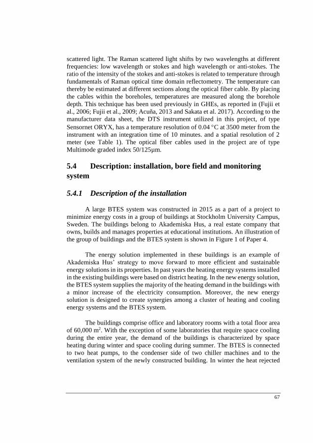
67
scattered light. The Raman scattered light shifts by two wavelengths at different
frequencies: low wavelength or stokes and high wavelength or anti-stokes. The
ratio of the intensity of the stokes and anti-stokes is related to temperature through
fundamentals of Raman optical time domain reflectometry. The temperature can
thereby be estimated at different sections along the optical fiber cable. By placing
the cables within the boreholes, temperatures are measured along the borehole
depth. This technique has been used previously in GHEs, as reported in (Fujii et
al., 2006; Fujii et al., 2009; Acuña, 2013 and Sakata et al. 2017). According to the
manufacturer data sheet, the DTS instrument utilized in this project, of type
Sensornet ORYX, has a temperature resolution of 0.04 C at 3500 meter from the
instrument with an integration time of 10 minutes. and a spatial resolution of 2
meter (see Table 1). The optical fiber cables used in the project are of type
Multimode graded index 50/125µm.
5.4 Description: installation, bore field and monitoring
system
5.4.1 Description of the installation
A large BTES system was constructed in 2015 as a part of a project to
minimize energy costs in a group of buildings at Stockholm University Campus,
Sweden. The buildings belong to Akademiska Hus, a real estate company that
owns, builds and manages properties at educational institutions. An illustration of
the group of buildings and the BTES system is shown in Figure 1 of Paper 4.
The energy solution implemented in these buildings is an example of
Akademiska Hus’ strategy to move forward to more efficient and sustainable
energy solutions in its properties. In past years the heating energy systems installed
in the existing buildings were based on district heating. In the new energy solution,
the BTES system supplies the majority of the heating demand in the buildings with
a minor increase of the electricity consumption. Moreover, the new energy
solution is designed to create synergies among a cluster of heating and cooling
energy systems and the BTES system.
The buildings comprise office and laboratory rooms with a total floor area
of 60,000 m2. With the exception of some laboratories that require space cooling
during the entire year, the demand of the buildings is characterized by space
heating during winter and space cooling during summer. The BTES is connected
to two heat pumps, to the condenser side of two chiller machines and to the
ventilation system of the newly constructed building. In winter the heat rejected
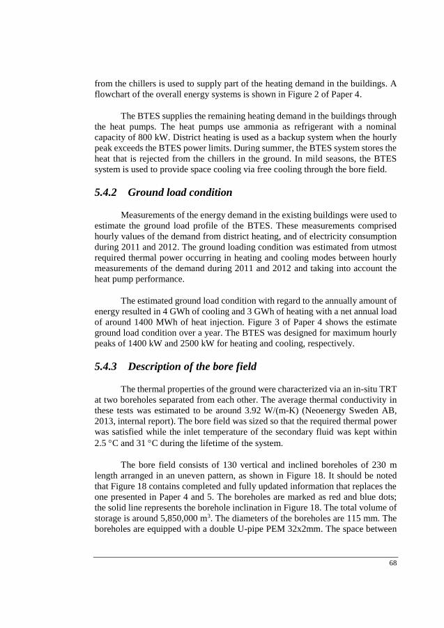
68
from the chillers is used to supply part of the heating demand in the buildings. A
flowchart of the overall energy systems is shown in Figure 2 of Paper 4.
The BTES supplies the remaining heating demand in the buildings through
the heat pumps. The heat pumps use ammonia as refrigerant with a nominal
capacity of 800 kW. District heating is used as a backup system when the hourly
peak exceeds the BTES power limits. During summer, the BTES system stores the
heat that is rejected from the chillers in the ground. In mild seasons, the BTES
system is used to provide space cooling via free cooling through the bore field.
5.4.2 Ground load condition
Measurements of the energy demand in the existing buildings were used to
estimate the ground load profile of the BTES. These measurements comprised
hourly values of the demand from district heating, and of electricity consumption
during 2011 and 2012. The ground loading condition was estimated from utmost
required thermal power occurring in heating and cooling modes between hourly
measurements of the demand during 2011 and 2012 and taking into account the
heat pump performance.
The estimated ground load condition with regard to the annually amount of
energy resulted in 4 GWh of cooling and 3 GWh of heating with a net annual load
of around 1400 MWh of heat injection. Figure 3 of Paper 4 shows the estimate
ground load condition over a year. The BTES was designed for maximum hourly
peaks of 1400 kW and 2500 kW for heating and cooling, respectively.
5.4.3 Description of the bore field
The thermal properties of the ground were characterized via an in-situ TRT
at two boreholes separated from each other. The average thermal conductivity in
these tests was estimated to be around 3.92 W/(m-K) (Neoenergy Sweden AB,
2013, internal report). The bore field was sized so that the required thermal power
was satisfied while the inlet temperature of the secondary fluid was kept within
2.5 C and 31 C during the lifetime of the system.
The bore field consists of 130 vertical and inclined boreholes of 230 m
length arranged in an uneven pattern, as shown in Figure 18. It should be noted
that Figure 18 contains completed and fully updated information that replaces the
one presented in Paper 4 and 5. The boreholes are marked as red and blue dots;
the solid line represents the borehole inclination in Figure 18. The total volume of
storage is around 5,850,000 m3. The diameters of the boreholes are 115 mm. The
boreholes are equipped with a double U-pipe PEM 32x2mm. The space between
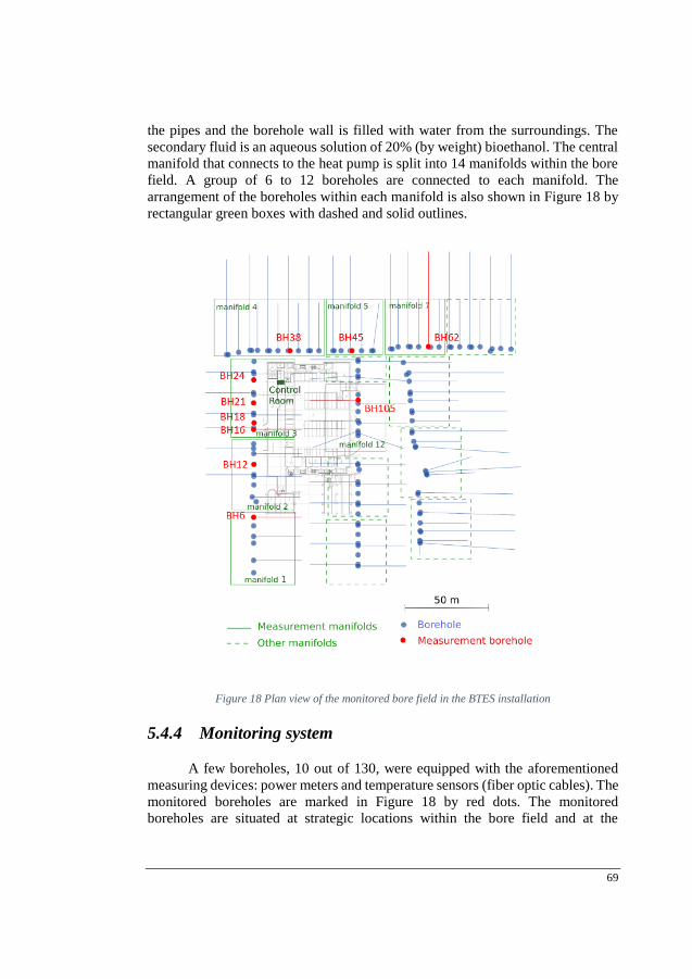
69
the pipes and the borehole wall is filled with water from the surroundings. The
secondary fluid is an aqueous solution of 20% (by weight) bioethanol. The central
manifold that connects to the heat pump is split into 14 manifolds within the bore
field. A group of 6 to 12 boreholes are connected to each manifold. The
arrangement of the boreholes within each manifold is also shown in Figure 18 by
rectangular green boxes with dashed and solid outlines.
Figure 18 Plan view of the monitored bore field in the BTES installation
5.4.4 Monitoring system
A few boreholes, 10 out of 130, were equipped with the aforementioned
measuring devices: power meters and temperature sensors (fiber optic cables). The
monitored boreholes are marked in Figure 18 by red dots. The monitored
boreholes are situated at strategic locations within the bore field and at the
70
periphery of the control room providing a detailed monitoring of the response of
the half upper part of the bore field. The monitored boreholes and their
corresponding manifolds were equipped with power meters, which were located
at the monitoring well. The measurements of the power meters are recorded every
minute. Figure 19 shows a sketch of the measuring procedure of the power
measurements in the measurement well.
Figure 19 Measuring procedure of power measurements in the monitored manifold and boreholes
along with some pictures of bore field components during their installation.
The secondary fluid is pumped out from the heat pump and distributed to
each manifold in the bore field. The route that the fluid follows is schematised in
Figure 19 with figures 1 to 9 as explained next. Before the secondary fluid enters
the manifold, volume flow rate and temperature at the inlet and outlet piping of
the manifold are measured at the measurement well (1 2). Then, the flow travels
to the manifold where the flow splits equally (3) and distributes to each borehole.
Before the secondary fluid enters the monitored borehole, it returns to the
measurement well and passes through its power meter (4) so that temperatures and
71
volume flow rate of the secondary fluid are measured. Then, the fluid circulates
along the GHE (5). When the fluid existing the monitored GHE, the fluid returns
first to the measurement well (6) where the outlet temperature of the monitored
borehole is measured. Then, the fluid travels to the manifold (7) and it mixes with
the fluid coming back from the remaning boreholes in the manifold. The fluid
returns back (8 9) to the heat pump, passing first again through the measurement
well at which the outlet temperature of the monitored manifold is measured. Figure
19 also shows some pictures of the components in the manifold that were taken
during their installation.
The monitored boreholes were also equipped with optical fiber cables
acting as temperature sensors, as explained above. Figure 5 of Paper 4 shows a set
of pictures during the installations of the cables in one of the boreholes. The optical
fiber cable was placed separately in each borehole, outside the GHE pipes.
The DTS instrument has four channels to which four fiber cables are
connected.
The fiber optical cable contains four fibers, but only two of them were used
in this arrangement. For connecting the fibers cables embedded in two boreholes
and to the DTS instrument, the continuous fiber cable was assembled by splicing
(welding) two of the fibers in the cable of one borehole by a series connection to
the corresponding two fibers of the cable in the neighboring borehole. The splice
was carried out in a junction box. Then, an end-loop connection was assembled
(fibers are spliced to each other) in one borehole. The other borehole connected in
series to the corresponding two fibers in an auxiliary cable that traveled from the
bore field to the DTS instrument. The DTS instrument is located indoors. An
example of the splice-fiber scheme, known as duplex arrangement (Hausner et al.,
2011), in two of the monitored boreholes in channel 3 is shown in Figure 20 (a).
Similar procedure was carried out in channel 1, 2 and 4, their splice-fiber schemes
are reported in Figure 58, 59 and 60, respectively, of the Appendix B.2.
The setting of the DTS instrument integration time is every ten minutes per
channel, and in space, every 1 meter. The the DTS data is recorded with a 40
minute interval for each channel. An example of the temperature measurement
recorded along the fiber cable length is shown in Figure 20 (b) for channel 3. The
DTS measurements were post-processed to identify the length of the fiber cable
relative to the borehole. The identification of the length intervals relative to the
monitored boreholes was done by the information of the fiber cable path and taking
advantage of reference sections. The reference sections are extra lengths of cable
reserved before and after the junction box. By placing the reference sections in
thermal baths with a known temperature, fiber cables reflected the temperature at
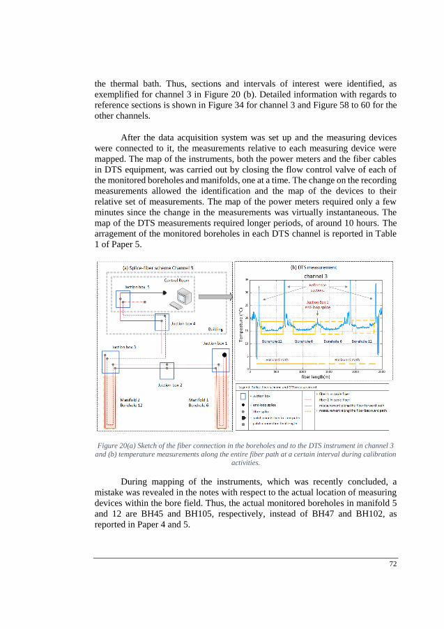
72
the thermal bath. Thus, sections and intervals of interest were identified, as
exemplified for channel 3 in Figure 20 (b). Detailed information with regards to
reference sections is shown in Figure 34 for channel 3 and Figure 58 to 60 for the
other channels.
After the data acquisition system was set up and the measuring devices
were connected to it, the measurements relative to each measuring device were
mapped. The map of the instruments, both the power meters and the fiber cables
in DTS equipment, was carried out by closing the flow control valve of each of
the monitored boreholes and manifolds, one at a time. The change on the recording
measurements allowed the identification and the map of the devices to their
relative set of measurements. The map of the power meters required only a few
minutes since the change in the measurements was virtually instantaneous. The
map of the DTS measurements required longer periods, of around 10 hours. The
arragement of the monitored boreholes in each DTS channel is reported in Table
1 of Paper 5.
Figure 20(a) Sketch of the fiber connection in the boreholes and to the DTS instrument in channel 3
and (b) temperature measurements along the entire fiber path at a certain interval during calibration
activities.
During mapping of the instruments, which was recently concluded, a
mistake was revealed in the notes with respect to the actual location of measuring
devices within the bore field. Thus, the actual monitored boreholes in manifold 5
and 12 are BH45 and BH105, respectively, instead of BH47 and BH102, as
reported in Paper 4 and 5.
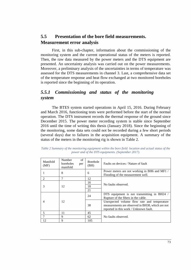
73
5.5 Presentation of the bore field measurements.
Measurement error analysis
First, in this sub-chapter, information about the commissioning of the
monitoring system and the current operational status of the meters is reported.
Then, the raw data measured by the power meters and the DTS equipment are
presented. An uncertainty analysis was carried out on the power measurements.
Moreover, a preliminary analysis of the uncertainties in terms of temperature was
assessed for the DTS measurements in channel 3. Last, a comprehensive data set
of the temperature response and heat flow exchanged at two monitored boreholes
is reported since the beginning of its operation.
5.5.1 Commissioning and status of the monitoring
system
The BTES system started operations in April 15, 2016. During February
and March 2016, functioning tests were performed before the start of the normal
operation. The DTS instrument records the thermal response of the ground since
December 2015. The power meter recording system is stable since September
2016 until the time of writing this thesis (January 2018). Since the beginning of
the monitoring, some data sets could not be recorded during a few short periods
(several days) due to failures in the acquisition equipment. A summary of the
status of the meters in the monitoring rig is shown in Table 2.
Table 2 Summary of the monitoring equipment within the bore field: location and actual status of the
power and of the DTS equipments. (September 2017).
Manifold
(MF)
Number of
boreholes per manifold
Borehole
(BH) Faults on devices / Nature of fault
1 8 6 Power meters are not working in BH6 and MF1 /
Flooding of the measurement well.
2 7 12
No faults observed. 3 12
16
18
21
4 12
24 DTS equipment is not transmitting in BH24 /
Rupture of the fibers in the cable.
38
Unexpected volume flow rate and temperature
measurements are observed in BH38, which are not
reported in this work / Unknown fault.
5 11 45
No faults observed. 7 9 62
12 9 105
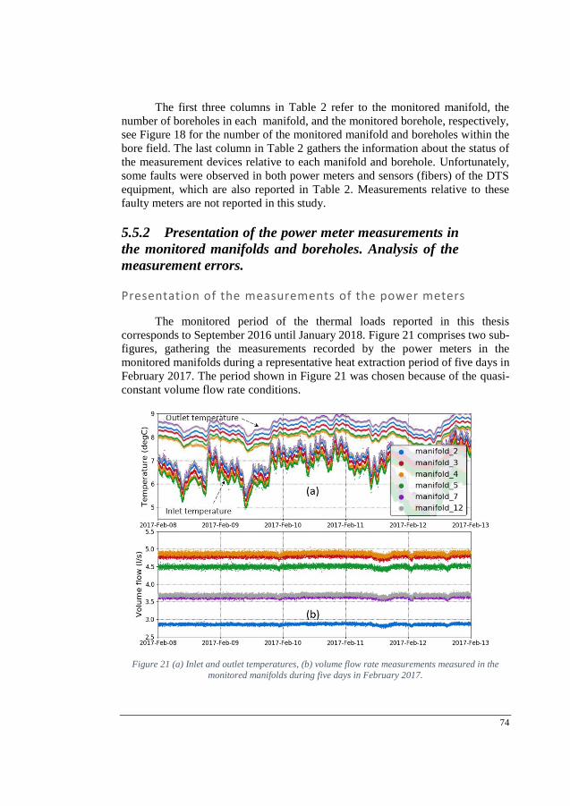
74
The first three columns in Table 2 refer to the monitored manifold, the
number of boreholes in each manifold, and the monitored borehole, respectively,
see Figure 18 for the number of the monitored manifold and boreholes within the
bore field. The last column in Table 2 gathers the information about the status of
the measurement devices relative to each manifold and borehole. Unfortunately,
some faults were observed in both power meters and sensors (fibers) of the DTS
equipment, which are also reported in Table 2. Measurements relative to these
faulty meters are not reported in this study.
5.5.2 Presentation of the power meter measurements in
the monitored manifolds and boreholes. Analysis of the
measurement errors.
Presentation of the measurements of the power meters
The monitored period of the thermal loads reported in this thesis
corresponds to September 2016 until January 2018. Figure 21 comprises two sub-
figures, gathering the measurements recorded by the power meters in the
monitored manifolds during a representative heat extraction period of five days in
February 2017. The period shown in Figure 21 was chosen because of the quasi-
constant volume flow rate conditions.
Figure 21 (a) Inlet and outlet temperatures, (b) volume flow rate measurements measured in the
monitored manifolds during five days in February 2017.
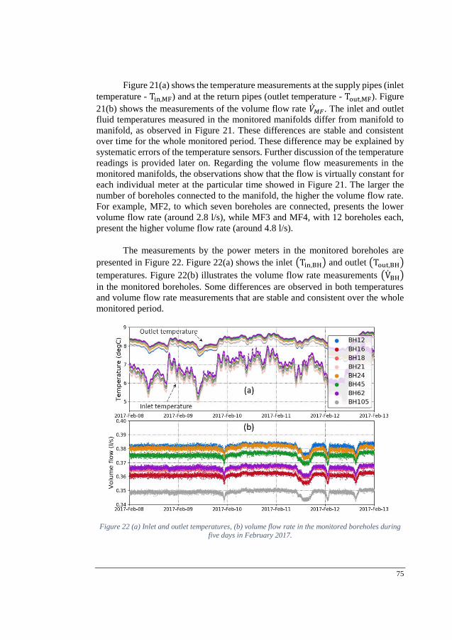
75
Figure 21(a) shows the temperature measurements at the supply pipes (inlet
temperature - Tin,MF) and at the return pipes (outlet temperature - Tout,MF). Figure
21(b) shows the measurements of the volume flow rate ��𝑀𝐹. The inlet and outlet
fluid temperatures measured in the monitored manifolds differ from manifold to
manifold, as observed in Figure 21. These differences are stable and consistent
over time for the whole monitored period. These difference may be explained by
systematic errors of the temperature sensors. Further discussion of the temperature
readings is provided later on. Regarding the volume flow measurements in the
monitored manifolds, the observations show that the flow is virtually constant for
each individual meter at the particular time showed in Figure 21. The larger the
number of boreholes connected to the manifold, the higher the volume flow rate.
For example, MF2, to which seven boreholes are connected, presents the lower
volume flow rate (around 2.8 l/s), while MF3 and MF4, with 12 boreholes each,
present the higher volume flow rate (around 4.8 l/s).
The measurements by the power meters in the monitored boreholes are
presented in Figure 22. Figure 22(a) shows the inlet (Tin,BH) and outlet (Tout,BH)
temperatures. Figure 22(b) illustrates the volume flow rate measurements (VBH)
in the monitored boreholes. Some differences are observed in both temperatures
and volume flow rate measurements that are stable and consistent over the whole
monitored period.
Figure 22 (a) Inlet and outlet temperatures, (b) volume flow rate in the monitored boreholes during five days in February 2017.
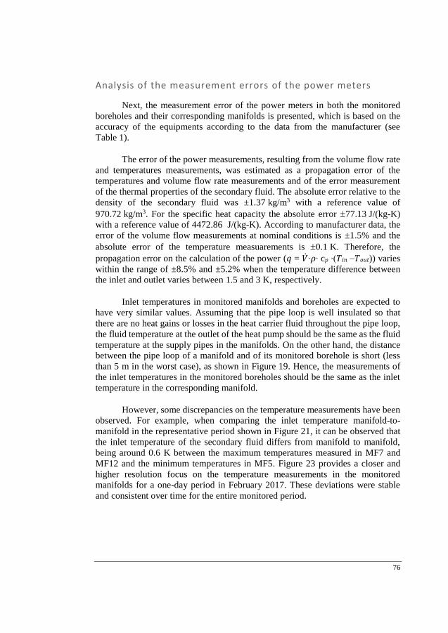
76
Analysis of the measurement errors of the power meters
Next, the measurement error of the power meters in both the monitored
boreholes and their corresponding manifolds is presented, which is based on the
accuracy of the equipments according to the data from the manufacturer (see
Table 1).
The error of the power measurements, resulting from the volume flow rate
and temperatures measurements, was estimated as a propagation error of the
temperatures and volume flow rate measurements and of the error measurement
of the thermal properties of the secondary fluid. The absolute error relative to the
density of the secondary fluid was ±1.37 kg/m3 with a reference value of
970.72 kg/m3. For the specific heat capacity the absolute error 77.13 J/(kg-K)
with a reference value of 4472.86 J/(kg-K). According to manufacturer data, the
error of the volume flow measurements at nominal conditions is ±1.5% and the
absolute error of the temperature measuarements is 0.1 K. Therefore, the
propagation error on the calculation of the power (𝑞 = ��∙𝜌∙ c𝑝 ∙(𝑇𝑖𝑛 –𝑇𝑜𝑢𝑡)) varies
within the range of ±8.5% and ±5.2% when the temperature difference between
the inlet and outlet varies between 1.5 and 3 K, respectively.
Inlet temperatures in monitored manifolds and boreholes are expected to
have very similar values. Assuming that the pipe loop is well insulated so that
there are no heat gains or losses in the heat carrier fluid throughout the pipe loop,
the fluid temperature at the outlet of the heat pump should be the same as the fluid
temperature at the supply pipes in the manifolds. On the other hand, the distance
between the pipe loop of a manifold and of its monitored borehole is short (less
than 5 m in the worst case), as shown in Figure 19. Hence, the measurements of
the inlet temperatures in the monitored boreholes should be the same as the inlet
temperature in the corresponding manifold.
However, some discrepancies on the temperature measurements have been
observed. For example, when comparing the inlet temperature manifold-to-
manifold in the representative period shown in Figure 21, it can be observed that
the inlet temperature of the secondary fluid differs from manifold to manifold,
being around 0.6 K between the maximum temperatures measured in MF7 and
MF12 and the minimum temperatures in MF5. Figure 23 provides a closer and
higher resolution focus on the temperature measurements in the monitored
manifolds for a one-day period in February 2017. These deviations were stable
and consistent over time for the entire monitored period.
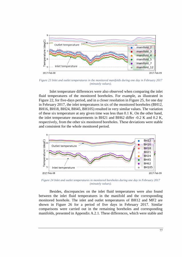
77
Figure 23 Inlet and outlet temperatures in the monitored manifolds during one day in February 2017 (minutely values).
Inlet temperature differences were also observed when comparing the inlet
fluid temperatures of the monitored boreholes. For example, as illustrated in
Figure 22, for five-days period, and in a closer resolution in Figure 25, for one day
in February 2017, the inlet temperatures in six of the monitored boreholes (BH12,
BH16, BH18, BH24, BH45, BH105) resulted in very similar values. The variation
of these six temperature at any given time was less than 0.1 K. On the other hand,
the inlet temperature measurements in BH21 and BH62 differ -0.2 K and 0.2 K,
respectively, from the other six monitored boreholes. These deviations were stable
and consistent for the whole monitored period.
Figure 24 Inlet and outlet temperatures in monitored boreholes during one day in February 2017
(minutely values).
Besides, discrepancies on the inlet fluid temperatures were also found
between the inlet fluid temperatures in the manifold and the corresponding
monitored borehole. The inlet and outlet temperatures of BH12 and MF2 are
shown in Figure 26 for a period of five days in February 2017. Similar
comparisons were carried out in the remaining boreholes and corresponding
manifolds, presented in Appendix A.2.1. These differences, which were stable and
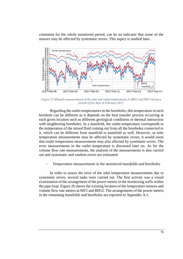
78
consistent for the whole monitored period, can be an indicator that some of the
sensors may be affected by systematic errors. This aspect is studied later.
Figure 25 Minutely measurements of the inlet and outlet temperatures in BH12 and MF2 during a period of five days in February 2017.
Regarding the outlet temperatures in the boreholes, this temperature in each
borehole can be different as it depends on the heat transfer process occurring at
each given location such as different geological conditions or thermal interaction
with neighboring boreholes. In a manifold, the outlet temperature corresponds to
the temperature of the mixed fluid coming out from all the boreholes connected to
it, which can be different from manifold to manifold as well. However, as inlet
temperature measurements may be affected by systematic errors, it would seem
that outlet temperature measurements may also affected by systematic errors. The
error measurements in the outlet temperature is discussed later on. As for the
volume flow rate measurements, the analysis of the measurements is also carried
out and systematic and random errors are estimated.
Temperature measurements in the monitored manifolds and boreholes
In order to assess the error of the inlet temperature measurements due to
systematic errors, several tasks were carried out. The first activity was a visual
examination of the arrangement of the power meters in the monitoring wells within
the pipe loop. Figure 26 shows the existing location of the temperature sensors and
volume flow rate meters in MF2 and BH12. The arrangements of the power meters
in the remaining manifolds and boreholes are reported in Appendix A.1.
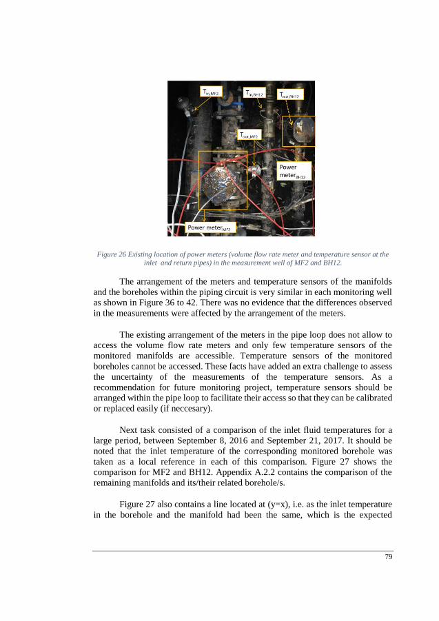
79
Figure 26 Existing location of power meters (volume flow rate meter and temperature sensor at the inlet and return pipes) in the measurement well of MF2 and BH12.
The arrangement of the meters and temperature sensors of the manifolds
and the boreholes within the piping circuit is very similar in each monitoring well
as shown in Figure 36 to 42. There was no evidence that the differences observed
in the measurements were affected by the arrangement of the meters.
The existing arrangement of the meters in the pipe loop does not allow to
access the volume flow rate meters and only few temperature sensors of the
monitored manifolds are accessible. Temperature sensors of the monitored
boreholes cannot be accessed. These facts have added an extra challenge to assess
the uncertainty of the measurements of the temperature sensors. As a
recommendation for future monitoring project, temperature sensors should be
arranged within the pipe loop to facilitate their access so that they can be calibrated
or replaced easily (if neccesary).
Next task consisted of a comparison of the inlet fluid temperatures for a
large period, between September 8, 2016 and September 21, 2017. It should be
noted that the inlet temperature of the corresponding monitored borehole was
taken as a local reference in each of this comparison. Figure 27 shows the
comparison for MF2 and BH12. Appendix A.2.2 contains the comparison of the
remaining manifolds and its/their related borehole/s.
Figure 27 also contains a line located at (y=x), i.e. as the inlet temperature
in the borehole and the manifold had been the same, which is the expected
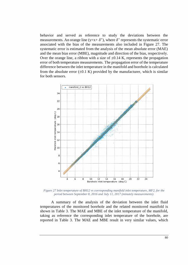
80
behavior and served as reference to study the deviations between the
measurements. An orange line (y=x+ 𝛿∗), where 𝛿∗ represents the systematic error
associated with the bias of the measurements also included in Figure 27. The
systematic error is estimated from the analysis of the mean absolute error (MAE)
and the mean bias error (MBE), magnitude and direction of the bias, respectively.
Over the orange line, a ribbon with a size of ±0.14 K, represents the propagation
error of both temperature measurements. The propagation error of the temperature
difference between the inlet temperature in the manifold and borehole is calculated
from the absolute error (0.1 K) provided by the manufacturer, which is similar
for both sensors.
Figure 27 Inlet temperature of BH12 vs corresponding manifold inlet temperature, MF2, for the
period between September 8, 2016 and July 11, 2017 (minutely measurements).
A summary of the analysis of the deviation between the inlet fluid
temperatures of the monitored borehole and the related monitored manifold is
shown in Table 3. The MAE and MBE of the inlet temperature of the manifold,
taking as reference the corresponding inlet temperature of the borehole, are
reported in Table 3. The MAE and MBE result in very similar values, which
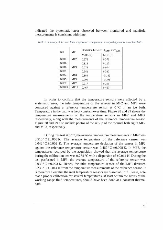
81
indicated the systematic error observed between monitored and manifold
measurements is consistent with time.
Table 3 Summary of the inlet fluid temperature comparison: manifold against relative borehole.
BH MF Deviation between Tin,MF vs Tin,BH
MAE (K) MBE (K)
BH12 MF2 0.376 0.376
BH16
MF3
0.118 0.117
BH18 0.076 0.074
BH21 0.341 0.340
BH24 MF4 0.184 -0.182
BH45 MF5 0.200 -0.195
BH62 MF7 0.217 0.216
BH105 MF12 0.467 0.467
In order to confirm that the temperature sensors were affected by a
systematic error, the inlet temperature of the sensors in MF2 and MF3 were
compared against a reference temperature sensor at 0 C in an ice bath.
Temperature in the bath was kept constant over time. Figure 28 and 29 shows the
temperature measurements of the temperature sensors in MF2 and MF3,
respectively, along with the measurements of the reference temperature sensor.
Figure 28 and 29 also include photos of the set-up of the thermal bath rig in MF2
and MF3, respectively.
During this test at 0 C, the average temperature measurements in MF2 was
0.510 C 0.008 K. The average temperature of the reference sensor was
0.042 C 0.002 K. The average temperature deviation of the sensor in MF2
against the reference temperature sensor was 0.467 C 0.008 K. In MF3, the
temperatures recorded by the acquisition showed that the average temperature
during the calibration test was 0.274 C with a dispersion of 0.014 K. During the
test performed in MF3, the average temperature of the reference sensor was
0.039 C 0.003 K. Hence, the inlet temperature sensor of the MF3 deviated
0.235 C 0.014 K from the temperature measurements of the reference sensor. It
is therefore clear that the inlet temperature sensors are biased at 0 C. Please, note
that a proper calibration for several temperatures, at least within the limits of the
working range fluid temperatures, should have been done at a constant thermal
bath.
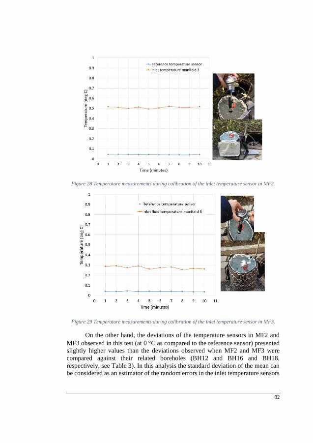
82
Figure 28 Temperature measurements during calibration of the inlet temperature sensor in MF2.
Figure 29 Temperature measurements during calibration of the inlet temperature sensor in MF3.
On the other hand, the deviations of the temperature sensors in MF2 and
MF3 observed in this test (at 0 C as compared to the reference sensor) presented
slightly higher values than the deviations observed when MF2 and MF3 were
compared against their related boreholes (BH12 and BH16 and BH18,
respectively, see Table 3). In this analysis the standard deviation of the mean can
be considered as an estimator of the random errors in the inlet temperature sensors
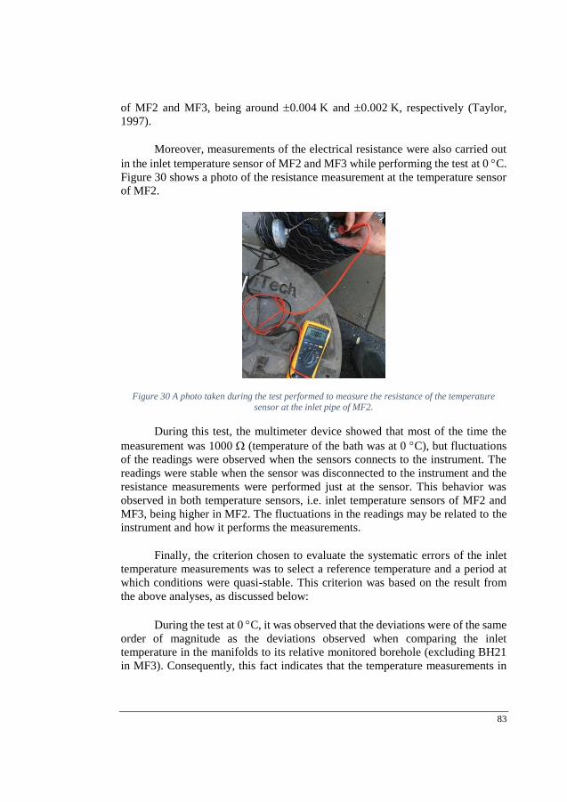
83
of MF2 and MF3, being around 0.004 K and 0.002 K, respectively (Taylor,
1997).
Moreover, measurements of the electrical resistance were also carried out
in the inlet temperature sensor of MF2 and MF3 while performing the test at 0 C.
Figure 30 shows a photo of the resistance measurement at the temperature sensor
of MF2.
Figure 30 A photo taken during the test performed to measure the resistance of the temperature sensor at the inlet pipe of MF2.
During this test, the multimeter device showed that most of the time the
measurement was 1000 (temperature of the bath was at 0 C), but fluctuations
of the readings were observed when the sensors connects to the instrument. The
readings were stable when the sensor was disconnected to the instrument and the
resistance measurements were performed just at the sensor. This behavior was
observed in both temperature sensors, i.e. inlet temperature sensors of MF2 and
MF3, being higher in MF2. The fluctuations in the readings may be related to the
instrument and how it performs the measurements.
Finally, the criterion chosen to evaluate the systematic errors of the inlet
temperature measurements was to select a reference temperature and a period at
which conditions were quasi-stable. This criterion was based on the result from
the above analyses, as discussed below:
During the test at 0 C, it was observed that the deviations were of the same
order of magnitude as the deviations observed when comparing the inlet
temperature in the manifolds to its relative monitored borehole (excluding BH21
in MF3). Consequently, this fact indicates that the temperature measurements in
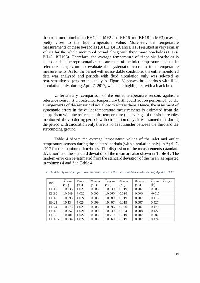
84
the monitored boreholes (BH12 in MF2 and BH16 and BH18 in MF3) may be
pretty close to the true temperature value. Moreover, the temperature
measurements of these boreholes (BH12, BH16 and BH18) resulted in very similar
values for the whole monitored period along with three more boreholes (BH24,
BH45, BH105). Therefore, the average temperature of these six boreholes is
considered as the representative measurement of the inlet temperature and as the
reference temperature to evaluate the systematic errors in inlet temperature
measurements. As for the period with quasi-stable conditions, the entire monitored
data was analyzed and periods with fluid circulation only was selected as
representative to perform this analysis. Figure 31 shows these periods with fluid
circulation only, during April 7, 2017, which are highlighted with a black box.
Unfortunately, comparison of the outlet temperature sensors against a
reference sensor at a controlled temperature bath could not be performed, as the
arrangements of the sensor did not allow to access them. Hence, the assesment of
systematic errors in the outlet temperature measurements is estimated from the
comparison with the reference inlet temperature (i.e. average of the six boreholes
mentioned above) during periods with circulation only. It is assumed that during
the period with circulation only there is no heat transfer between the fluid and the
surrounding ground.
Table 4 shows the average temperature values of the inlet and outlet
temperature sensors during the selected periods (with circulation only) in April 7,
2017 for the monitored boreholes. The dispersion of the measurements (standard
deviation) and the standard deviation of the mean are also shown in Table 4 . The
random error can be estimated from the standard deviation of the mean, as reported
in columns 4 and 7 in Table 4.
Table 4 Analysis of temperature measurements in the monitored boreholes during April 7, 2017 .
BH 𝑇𝑖𝑛,𝐵𝐻
(C)
𝜎𝑇𝑖𝑛,𝐵𝐻
(C)
𝜎𝑇𝑖𝑛,𝐵𝐻
(C)
𝑇𝑜𝑢𝑡,𝐵𝐻
(C)
𝜎𝑇𝑜𝑢𝑡,𝐵𝐻
(C)
𝜎𝑇𝑜𝑢𝑡,𝐵𝐻
(C)
𝑇𝑖𝑛,𝐵𝐻 − 𝑇𝑜𝑢𝑡,𝐵𝐻
(K)
BH12 10.633 0.023 0.008 10.530 0.019 0.007 0.103
BH16 10.649 0.023 0.008 10.666 0.018 0.006 -0.017
BH18 10.695 0.024 0.008 10.680 0.019 0.007 0.015
BH21 10.434 0.024 0.009 10.407 0.019 0.007 0.027
BH24 10.675 0.023 0.008 10.596 0.020 0.007 0.079
BH45 10.657 0.026 0.009 10.630 0.024 0.008 0.027
BH62 10.901 0.024 0.008 10.719 0.019 0.007 0.182
BH105 10.634 0.024 0.008 10.560 0.019 0.007 0.074
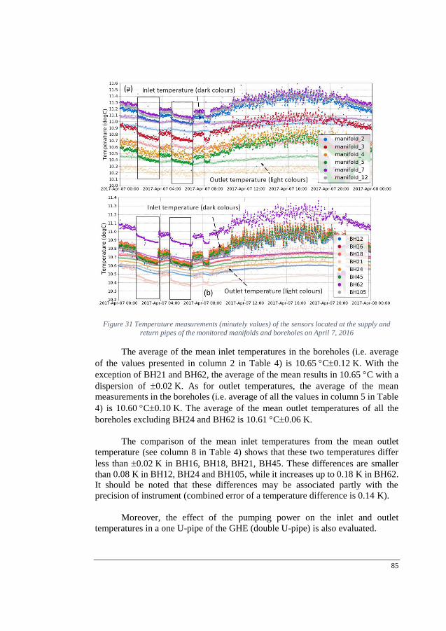
85
Figure 31 Temperature measurements (minutely values) of the sensors located at the supply and
return pipes of the monitored manifolds and boreholes on April 7, 2016
The average of the mean inlet temperatures in the boreholes (i.e. average
of the values presented in column 2 in Table 4) is 10.65 C0.12 K. With the
exception of BH21 and BH62, the average of the mean results in 10.65 C with a
dispersion of 0.02 K. As for outlet temperatures, the average of the mean
measurements in the boreholes (i.e. average of all the values in column 5 in Table
4) is 10.60 C0.10 K. The average of the mean outlet temperatures of all the
boreholes excluding BH24 and BH62 is 10.61 C0.06 K.
The comparison of the mean inlet temperatures from the mean outlet
temperature (see column 8 in Table 4) shows that these two temperatures differ
less than 0.02 K in BH16, BH18, BH21, BH45. These differences are smaller
than 0.08 K in BH12, BH24 and BH105, while it increases up to 0.18 K in BH62.
It should be noted that these differences may be associated partly with the
precision of instrument (combined error of a temperature difference is 0.14 K).
Moreover, the effect of the pumping power on the inlet and outlet
temperatures in a one U-pipe of the GHE (double U-pipe) is also evaluated.
86
The pumping power is calculated as Pf = V ∙ ∆P1000⁄ where ∆P represents
the pressure loss of the overall piping circuit. In this study the total pressure loss
of the overall circuit is estimated from the pressure loss of each loop, i.e. each U-
pipe. Hence, the pressure loss in a loop is calculated as ∆Ploop = lf,loop ∙ ρ ∙g where
is the density of the secondary fluid (972 kg/m3), g is the gravitational constant
(9.82 m/s2).The term lf,loop represents the head loss per loop lf,loop = fLloop
Dpipe∙
ν2
g
with Lloop being the total length of the downward and upward in a U-pipe, i.e 460
m, Dpipe is the diameter of the U-pipe, ν is the velocity of the fluid (m/s) in one U-
pie, i.e V/2
Apipe. The pressure loss in a loop is 6 W. The impact of the pumping power
on the temperature differences between the inlet and outlet temperature in a loop
(i.e. in one U-pipe of the GHE) is around 0.007 K. Hence, the effect of the pumping
power has a minimal impact on the differences between the inlet and outlet
temperatures in each borehole.
Next, the variation of the temperature measurements at each given time
during the highlighted periods shown in Figure 31 are analyzed against the
reference temperature (Tref,BH is the average value of the inlet temperature
measurements in BH12, BH16, BH18, BH24, BH45, BH105 at any instant of
time).
In Table 5, column 2 and 3 shows the MAE and MBE of the inlet
temperature measurements obtained from the comparasion against the reference
temperature. The MAE and MBE of the oulet temperature measurements is
presented in column 5 and 6 in Table 5. The MAE and MBE are of the same
magnitude in each individual temperature set measurements for both inlet and
outlet temperature analyses The MAE and MBE are used in this study as an
indicator of the magnitude and direction of the systematic error (bias in the
measurements). It should be noted that the MAE of the inlet and outlet temperature
measurements of BH16, BH18, BH21, BH24 and BH45 differ less than 0.05 K,
which indicates that the systematic errors in the measurements of are of the same
magnitude (this fact will have a minimal impact in the power calculations as it is
the result of the temperature difference between these two measurements). The
difference between the MAE of the inlet and outlet mean temperatures in BH12
and BH105 is less than 0.1 K, being with the margin of the propagation errors.
However, the bias of the inlet and outlet temperature measurements is not of the
same magnitude in BH62, with a larger systematic error in the inlet temperature
measurements.
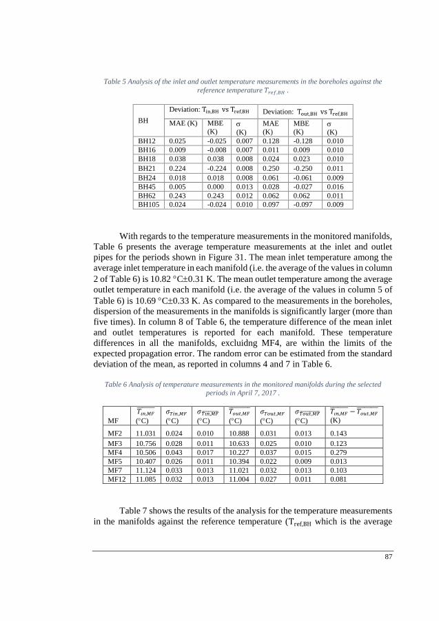
87
Table 5 Analysis of the inlet and outlet temperature measurements in the boreholes against the
reference temperature 𝑇𝑟𝑒𝑓,𝐵𝐻 .
BH
Deviation: Tin,BH vs Tref,BH Deviation: Tout,BH vs Tref,BH
MAE (K) MBE
(K) (K)
MAE
(K)
MBE
(K) (K)
BH12 0.025 -0.025 0.007 0.128 -0.128 0.010
BH16 0.009 -0.008 0.007 0.011 0.009 0.010
BH18 0.038 0.038 0.008 0.024 0.023 0.010
BH21 0.224 -0.224 0.008 0.250 -0.250 0.011
BH24 0.018 0.018 0.008 0.061 -0.061 0.009
BH45 0.005 0.000 0.013 0.028 -0.027 0.016
BH62 0.243 0.243 0.012 0.062 0.062 0.011
BH105 0.024 -0.024 0.010 0.097 -0.097 0.009
With regards to the temperature measurements in the monitored manifolds,
Table 6 presents the average temperature measurements at the inlet and outlet
pipes for the periods shown in Figure 31. The mean inlet temperature among the
average inlet temperature in each manifold (i.e. the average of the values in column
2 of Table 6) is 10.82 C0.31 K. The mean outlet temperature among the average
outlet temperature in each manifold (i.e. the average of the values in column 5 of
Table 6) is 10.69 C0.33 K. As compared to the measurements in the boreholes,
dispersion of the measurements in the manifolds is significantly larger (more than
five times). In column 8 of Table 6, the temperature difference of the mean inlet
and outlet temperatures is reported for each manifold. These temperature
differences in all the manifolds, excluidng MF4, are within the limits of the
expected propagation error. The random error can be estimated from the standard
deviation of the mean, as reported in columns 4 and 7 in Table 6.
Table 6 Analysis of temperature measurements in the monitored manifolds during the selected
periods in April 7, 2017 .
MF
𝑇𝑖𝑛,𝑀𝐹
(C)
𝜎𝑇𝑖𝑛,𝑀𝐹
(C)
𝜎𝑇𝑖𝑛,𝑀𝐹
(C)
𝑇𝑜𝑢𝑡,𝑀𝐹
(C)
𝜎𝑇𝑜𝑢𝑡,𝑀𝐹
(C)
𝜎𝑇𝑜𝑢𝑡,𝑀𝐹
(C)
𝑇𝑖𝑛,𝑀𝐹 − 𝑇𝑜𝑢𝑡,𝑀𝐹
(K)
MF2 11.031 0.024 0.010 10.888 0.031 0.013 0.143
MF3 10.756 0.028 0.011 10.633 0.025 0.010 0.123
MF4 10.506 0.043 0.017 10.227 0.037 0.015 0.279
MF5 10.407 0.026 0.011 10.394 0.022 0.009 0.013
MF7 11.124 0.033 0.013 11.021 0.032 0.013 0.103
MF12 11.085 0.032 0.013 11.004 0.027 0.011 0.081
Table 7 shows the results of the analysis for the temperature measurements
in the manifolds against the reference temperature (Tref,BH which is the average
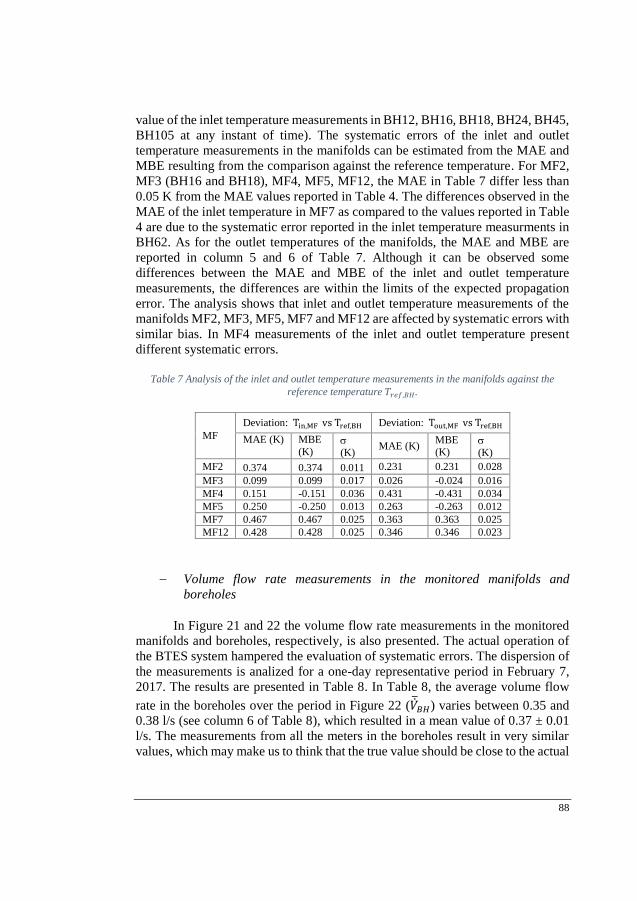
88
value of the inlet temperature measurements in BH12, BH16, BH18, BH24, BH45,
BH105 at any instant of time). The systematic errors of the inlet and outlet
temperature measurements in the manifolds can be estimated from the MAE and
MBE resulting from the comparison against the reference temperature. For MF2,
MF3 (BH16 and BH18), MF4, MF5, MF12, the MAE in Table 7 differ less than
0.05 K from the MAE values reported in Table 4. The differences observed in the
MAE of the inlet temperature in MF7 as compared to the values reported in Table
4 are due to the systematic error reported in the inlet temperature measurments in
BH62. As for the outlet temperatures of the manifolds, the MAE and MBE are
reported in column 5 and 6 of Table 7. Although it can be observed some
differences between the MAE and MBE of the inlet and outlet temperature
measurements, the differences are within the limits of the expected propagation
error. The analysis shows that inlet and outlet temperature measurements of the
manifolds MF2, MF3, MF5, MF7 and MF12 are affected by systematic errors with
similar bias. In MF4 measurements of the inlet and outlet temperature present
different systematic errors.
Table 7 Analysis of the inlet and outlet temperature measurements in the manifolds against the
reference temperature 𝑇𝑟𝑒𝑓,𝐵𝐻.
MF
Deviation: Tin,MF vs Tref,BH Deviation: Tout,MF vs Tref,BH
MAE (K) MBE
(K) (K)
MAE (K) MBE (K)
(K)
MF2 0.374 0.374 0.011 0.231 0.231 0.028
MF3 0.099 0.099 0.017 0.026 -0.024 0.016
MF4 0.151 -0.151 0.036 0.431 -0.431 0.034
MF5 0.250 -0.250 0.013 0.263 -0.263 0.012
MF7 0.467 0.467 0.025 0.363 0.363 0.025
MF12 0.428 0.428 0.025 0.346 0.346 0.023
Volume flow rate measurements in the monitored manifolds and
boreholes
In Figure 21 and 22 the volume flow rate measurements in the monitored
manifolds and boreholes, respectively, is also presented. The actual operation of
the BTES system hampered the evaluation of systematic errors. The dispersion of
the measurements is analized for a one-day representative period in February 7,
2017. The results are presented in Table 8. In Table 8, the average volume flow
rate in the boreholes over the period in Figure 22 (��𝐵𝐻) varies between 0.35 and
0.38 l/s (see column 6 of Table 8), which resulted in a mean value of 0.37 ± 0.01
l/s. The measurements from all the meters in the boreholes result in very similar
values, which may make us to think that the true value should be close to the actual
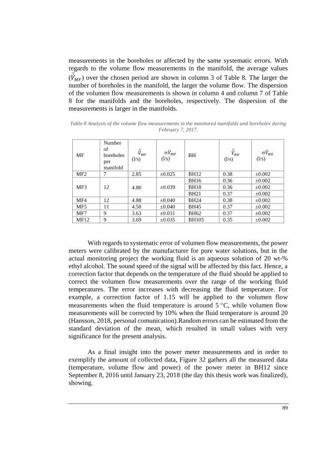
89
measurements in the boreholes or affected by the same systematic errors. With
regards to the volume flow measurements in the manifold, the average values
(��𝑀𝐹) over the chosen period are shown in column 3 of Table 8. The larger the
number of boreholes in the manifold, the larger the volume flow. The dispersion
of the volumen flow measurements is shown in column 4 and column 7 of Table
8 for the manifolds and the boreholes, respectively. The dispersion of the
measurements is larger in the manifolds.
Table 8 Analysis of the volume flow measurements in the monitored manifolds and boreholes during
February 7, 2017.
MF
Number
of boreholes
per
manifold
��𝑀𝐹 (l/s)
��𝑀𝐹 (l/s)
BH ��𝐵𝐻 (l/s)
��𝐵𝐻 (l/s)
MF2 7 2.85 ±0.025 BH12 0.38 ±0.002
MF3 12 4.80
±0.039
BH16 0.36 ±0.002
BH18 0.36 ±0.002
BH21 0.37 ±0.002
MF4 12 4.88 ±0.040 BH24 0.38 ±0.002
MF5 11 4.50 ±0.040 BH45 0.37 ±0.002
MF7 9 3.63 ±0.031 BH62 0.37 ±0.002
MF12 9 3.69 ±0.035 BH105 0.35 ±0.002
With regards to systematic error of volumen flow measurements, the power
meters were calibrated by the manufacturer for pure water solutions, but in the
actual monitoring project the working fluid is an aqueous solution of 20 wt-%
ethyl alcohol. The sound speed of the signal will be affected by this fact. Hence, a
correction factor that depends on the temperature of the fluid should be applied to
correct the volumen flow measurements over the range of the working fluid
temperatures. The error increases with decreasing the fluid temperature. For
example, a correction factor of 1.15 will be applied to the volumen flow
measurements when the fluid temperature is around 5 C, while volumen flow
measurements will be corrected by 10% when the fluid temperature is around 20
(Hansson, 2018, personal comunication).Random errors can be estimated from the
standard deviation of the mean, which resulted in small values with very
significance for the present analysis.
As a final insight into the power meter measurements and in order to
exemplify the amount of collected data, Figure 32 gathers all the measured data
(temperature, volume flow and power) of the power meter in BH12 since
September 8, 2016 until January 23, 2018 (the day this thesis work was finalized),
showing.
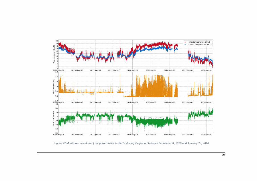
90
Figure 32 Monitored raw data of the power meter in BH12 during the period between September 8, 2016 and January 23, 2018
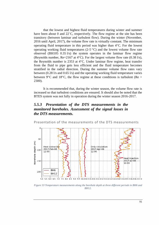
91
that the lowest and highest fluid temperatures during winter and summer
have been about 0 and 22˚C, respectively. The flow regime at the site has been
transitory (between laminar and turbulent flow). During the winter (November,
2016 until April, 2017), the volume flow rate is virtually constant. The minimum
operating fluid temperature in this period was higher than 4C. For the lowest
operating working fluid temperatures (2-5 C) and the lowest volume flow rate
observed (BH105 0.35 l/s) the system operates in the laminar flow regime
(Reynolds number, Re=2167 at 4C). For the largest volume flow rate (0.38 l/s),
the Reynolds number is 2353 at 4C. Under laminar flow regime, heat transfer
from the fluid to pipe gets less efficient and the fluid temperature becomes
stratified in the radial direction. During the summer volume flow rates vary
between (0.28 l/s and 0.65 l/s) and the operating working fluid temperature varies
between 9C and 18C, the flow regime at these conditions is turbulent (Re >
2300).
It is recommended that, during the winter season, the volume flow rate is
increased so that turbulent conditions are ensured. It should also be noted that the
BTES system was not fully in operation during the winter season 2016-2017.
5.5.3 Presentation of the DTS measurements in the
monitored boreholes. Assessment of the signal losses in
the DTS measurements.
Presentation of the measurements of the DTS measurements
Figure 33 Temperature measurements along the borehole depth at three different periods in BH6 and BH12.
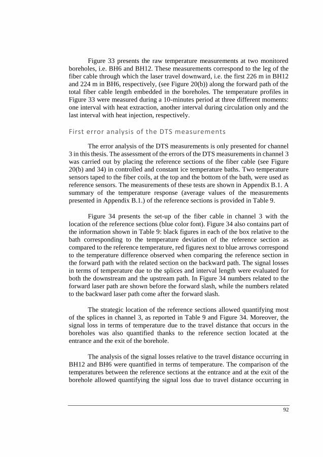
92
Figure 33 presents the raw temperature measurements at two monitored
boreholes, i.e. BH6 and BH12. These measurements correspond to the leg of the
fiber cable through which the laser travel downward, i.e. the first 226 m in BH12
and 224 m in BH6, respectively, (see Figure 20(b)) along the forward path of the
total fiber cable length embedded in the boreholes. The temperature profiles in
Figure 33 were measured during a 10-minutes period at three different moments:
one interval with heat extraction, another interval during circulation only and the
last interval with heat injection, respectively.
First error analysis of the DTS measurements
The error analysis of the DTS measurements is only presented for channel
3 in this thesis. The assessment of the errors of the DTS measurements in channel 3
was carried out by placing the reference sections of the fiber cable (see Figure
20(b) and 34) in controlled and constant ice temperature baths. Two temperature
sensors taped to the fiber coils, at the top and the bottom of the bath, were used as
reference sensors. The measurements of these tests are shown in Appendix B.1. A
summary of the temperature response (average values of the measurements
presented in Appendix B.1.) of the reference sections is provided in Table 9.
Figure 34 presents the set-up of the fiber cable in channel 3 with the
location of the reference sections (blue color font). Figure 34 also contains part of
the information shown in Table 9: black figures in each of the box relative to the
bath corresponding to the temperature deviation of the reference section as
compared to the reference temperature, red figures next to blue arrows correspond
to the temperature difference observed when comparing the reference section in
the forward path with the related section on the backward path. The signal losses
in terms of temperature due to the splices and interval length were evaluated for
both the downstream and the upstream path. In Figure 34 numbers related to the
forward laser path are shown before the forward slash, while the numbers related
to the backward laser path come after the forward slash.
The strategic location of the reference sections allowed quantifying most
of the splices in channel 3, as reported in Table 9 and Figure 34. Moreover, the
signal loss in terms of temperature due to the travel distance that occurs in the
boreholes was also quantified thanks to the reference section located at the
entrance and the exit of the borehole.
The analysis of the signal losses relative to the travel distance occurring in
BH12 and BH6 were quantified in terms of temperature. The comparison of the
temperatures between the reference sections at the entrance and at the exit of the
borehole allowed quantifying the signal loss due to travel distance occurring in
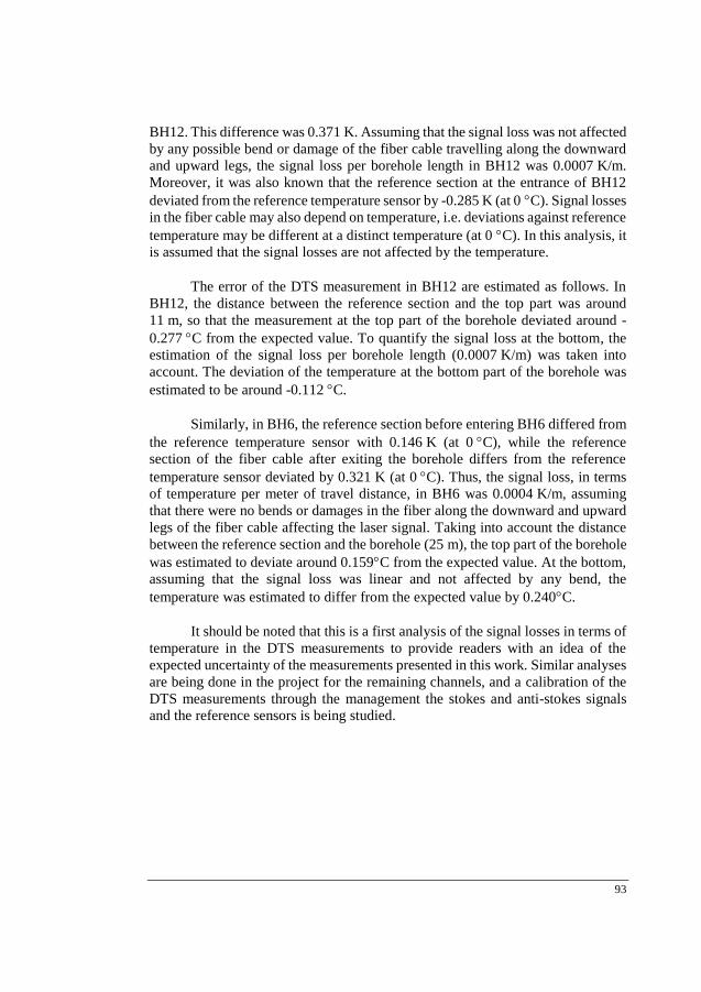
93
BH12. This difference was 0.371 K. Assuming that the signal loss was not affected
by any possible bend or damage of the fiber cable travelling along the downward
and upward legs, the signal loss per borehole length in BH12 was 0.0007 K/m.
Moreover, it was also known that the reference section at the entrance of BH12
deviated from the reference temperature sensor by -0.285 K (at 0 C). Signal losses
in the fiber cable may also depend on temperature, i.e. deviations against reference
temperature may be different at a distinct temperature (at 0 C). In this analysis, it
is assumed that the signal losses are not affected by the temperature.
The error of the DTS measurement in BH12 are estimated as follows. In
BH12, the distance between the reference section and the top part was around
11 m, so that the measurement at the top part of the borehole deviated around -
0.277 C from the expected value. To quantify the signal loss at the bottom, the
estimation of the signal loss per borehole length (0.0007 K/m) was taken into
account. The deviation of the temperature at the bottom part of the borehole was
estimated to be around -0.112 C.
Similarly, in BH6, the reference section before entering BH6 differed from
the reference temperature sensor with 0.146 K (at 0 C), while the reference
section of the fiber cable after exiting the borehole differs from the reference
temperature sensor deviated by 0.321 K (at 0 C). Thus, the signal loss, in terms
of temperature per meter of travel distance, in BH6 was 0.0004 K/m, assuming
that there were no bends or damages in the fiber along the downward and upward
legs of the fiber cable affecting the laser signal. Taking into account the distance
between the reference section and the borehole (25 m), the top part of the borehole
was estimated to deviate around 0.159C from the expected value. At the bottom,
assuming that the signal loss was linear and not affected by any bend, the
temperature was estimated to differ from the expected value by 0.240C.
It should be noted that this is a first analysis of the signal losses in terms of
temperature in the DTS measurements to provide readers with an idea of the
expected uncertainty of the measurements presented in this work. Similar analyses
are being done in the project for the remaining channels, and a calibration of the
DTS measurements through the management the stokes and anti-stokes signals
and the reference sensors is being studied.
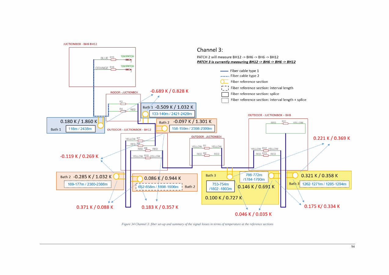
94
Figure 34 Channel 3: fiber set-up and summary of the signal losses in terms of temperature at the reference sections
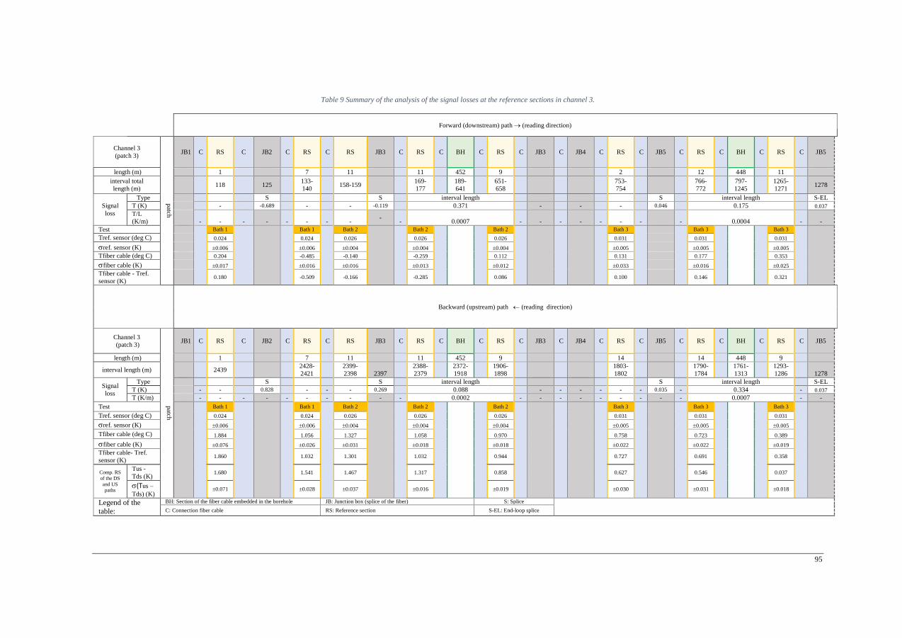
95
Table 9 Summary of the analysis of the signal losses at the reference sections in channel 3.
Forward (downstream) path (reading direction)
Channel 3
(patch 3)
patch
JB1 C RS C JB2 C RS C RS JB3 C RS C BH C RS C JB3 C JB4 C RS C JB5 C RS C BH C RS C JB5
length (m) 1 7 11 11 452 9 2 12 448 11
interval total
length (m) 118 125
133-
140 158-159
169-
177
189-
641
651-
658
753-
754
766-
772
797-
1245
1265-
1271 1278
Signal
loss
Type S S interval length S interval length S-EL
T (K) - -0.689 - - -0.119 0.371 - - - 0.046 0.175 0.037
T/L
(K/m) - - - - - - - - -
- 0.0007 - - - - - - - - 0.0004 - -
Test
Bath 1
Bath 1
Bath 2
Bath 2
Bath 2
Bath 3
Bath 3
Bath 3
Tref. sensor (deg C) 0.024 0.024 0.026 0.026 0.026 0.031 0.031 0.031
ref. sensor (K) 0.006 0.006 0.004 0.004 0.004 0.005 0.005 0.005
Tfiber cable (deg C) 0.204 -0.485 -0.140 -0.259 0.112 0.131 0.177 0.353
fiber cable (K) 0.017 0.016 0.016 0.013 0.012 0.033 0.016 0.025
Tfiber cable - Tref.
sensor (K) 0.180 -0.509 -0.166 -0.285 0.086 0.100 0.146 0.321
Backward (upstream) path (reading direction)
Channel 3
(patch 3)
patch
JB1 C RS C JB2 C RS C RS JB3 C RS C BH C RS C JB3 C JB4 C RS C JB5 C RS C BH C RS C JB5
length (m) 1 7 11 11 452 9 14 14 448 9
interval length (m)
2439
2428-
2421
2399-
2398 2397
2388-
2379
2372-
1918
1906-
1898
1803-
1802
1790-
1784
1761-
1313
1293-
1286 1278
Signal
loss
Type S S interval length S interval length S-EL
T (K) - - 0.828 - - - 0.269 0.088 - - - - - - 0.035 - 0.334 - 0.037
T (K/m) - - - - - - - - - - 0.0002 - - - - - - - - - 0.0007 - -
Test
Bath 1
Bath 1
Bath 2
Bath 2
Bath 2
Bath 3
Bath 3
Bath 3
Tref. sensor (deg C) 0.024 0.024 0.026 0.026 0.026 0.031 0.031 0.031
ref. sensor (K) 0.006 0.006 0.004 0.004 0.004 0.005 0.005 0.005
Tfiber cable (deg C) 1.884 1.056 1.327 1.058 0.970 0.758 0.723 0.389
fiber cable (K) 0.076 0.026 0.031 0.018 0.018 0.022 0.022 0.019
Tfiber cable- Tref.
sensor (K) 1.860 1.032 1.301 1.032 0.944 0.727 0.691 0.358
Comp. RS
of the DS
and US paths
Tus -
Tds (K) 1.680 1.541 1.467 1.317 0.858 0.627 0.546 0.037
(Tus –
Tds) (K) ±0.071 ±0.028 ±0.037 ±0.016 ±0.019 ±0.030 ±0.031 ±0.018
Legend of the
table:
BH: Section of the fiber cable embedded in the borehole JB: Junction box (splice of the fiber) S: Splice
C: Connection fiber cable RS: Reference section S-EL: End-loop splice
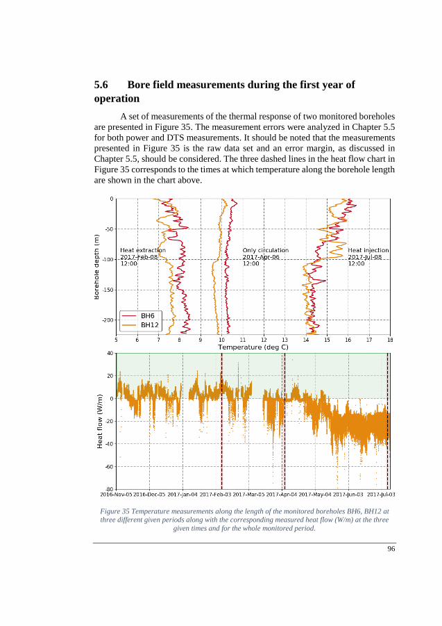
96
5.6 Bore field measurements during the first year of
operation
A set of measurements of the thermal response of two monitored boreholes
are presented in Figure 35. The measurement errors were analyzed in Chapter 5.5
for both power and DTS measurements. It should be noted that the measurements
presented in Figure 35 is the raw data set and an error margin, as discussed in
Chapter 5.5, should be considered. The three dashed lines in the heat flow chart in
Figure 35 corresponds to the times at which temperature along the borehole length
are shown in the chart above.
Figure 35 Temperature measurements along the length of the monitored boreholes BH6, BH12 at three different given periods along with the corresponding measured heat flow (W/m) at the three
given times and for the whole monitored period.
97
Figure 35 shows a particular behavior of the groundwater temperature at
about 100 m depth in BH12. Although the extracted power was rather low, Figure
35 shows the accordance between power meters and DTS, as well as how
grounwater temperatures outside the GHE pipes can vary with depth and time in
the monitored boreholes at this BTES site. These measurements are unique and
will contribute to further research during the coming years.
5.7 Conclusions
In order to pursue the final objective of this chapter, the implementation of
a monitoring set-up was first carried out. A comprehensive insight into power
(volume flow and temperature) measurements was provided for a multiple bore
field of a BTES system.
Relevant activities, full documentation and error analyses were reported,
which may be of interest for future monitoring projects and and for validating bore
field sizing methods. Power meters and a distributed temperature sensing
instrument with optical fiber cables were successfully installed and put into
operation. Measurements are being recorded since the monitoring system was
fully operational in September 2016.
Unique power measurements in manifolds and nine GHEs as well as
temperature profiles along the full depth on the groundwater side of the nine
boreholes were presented for the monitored period between September 2016 and
Januray 2018, together with an analysis of measurement errors of the power and
of the signal losses of the DTS temperature measurements.
The measurement errors of the power measurements was estimated to vary
between ±5.2% and ±9.5% when the difference between the inlet and the outlet is
around 3 K and 1.5 K, respectively. Systematic errors were estimated in
temperature and volume flow measurements in the manifolds and boreholes. A
correction factor should be applied to correct the volume flow measurements to
adjust the errors of the intrument for the actual working fluid (an aqueous solution
of 20 wt-% ethyl alcohol).
With regard to the DTS measurements, registered signal losses were
characterized through monitored temperatur in the reference sections with ice
baths (at 0 C) using the fiber loop connected to channel 3 of the DTS instrument.
The registered losses were also characterized at most of the splices and due to
travel distance in the monitored boreholes of channel 3. The error of the DTS
measurements in BH12 is estimated to deviate at the top around -0.277 C and -
0.122 C at the bottom. In BH6, at the top part of the borehole DTS measurements

98
are estimated to deviate around 0.159 C at the top part of the borehole and
0.240 C at the bottom part of the borehole. Given the complexity of this DTS
measurement system, a similar analysis for all DTS channels should be carried
out prior to adjusting or calibrating the measured data.
99
6. CONCLUSIONS
The investigations carried out during this Ph.D. study contributed to the
development of tools for the evaluation of the bore field response via the following
specific investigations:
1. A numerical model was developed with the particularity that the ground
conditions naturally controlled the heat transfer through the borehole
instead of imposing a boundary condition at the borehole wall. The model
also took into account the effect of the fluid-to-borehole wall thermal
resistance on the heat flux distribution along the borehole wall, which was
often disregarded.
The model used a fictitious highly conductive material to create a very
small temperature gradient occurring along the borehole length. Together with a
thin thermally resistive layer, defined at the borehole wall, the model accounted
for the effect of the borehole thermal resistance and and allows the bore field to
naturally controll the conditions at the borehole wall.
The proposed model was used to analyze the temperature and heat flux
distribution along the borehole length. Neither temperature profiles were uniform
nor the heat flux profiles were constant. It was proved that the unavoidable
borehole thermal resistance violates the assumption of uniform borehole wall
temperature, which is often assumed in mathematical models. Results from the
enhanced model serve as a reference to other approaches.
The model was also used to generate temperature responses with a
continuous total heat flow for multiple bore fields. Although there were no major
differencesbetween the proposed model and solutions based on a uniform borehole
temperature, deviations increased with number of boreholes. The model was also
used to illustrate and reciprocally validate the fluid temperature of two monitored
sites.
2. A general methodology for bore field sizing that calculates the maximum
required total bore field length for each arbitrary month during the lifetime
of the installations was developed.
The methodology calculates the total required bore field length for the first
year of operation or at any longer time. The proposed methodology allows to find
the optimum borehole spacing that results in the minimum total bore field for a
quasi-balanced ground load condition. The proposed methodology was
exemplified for a particular quasi-balanced load scenario, showing that the
100
maximum length can occur during the first year of operation and the optimum
borehole spacing.
A recommendation to include the first year of operation on the evaluation
of the total bore field length, as proposed in Equation12, was suggested to the bore
field sizing method in ASHRAE HandbookHVAC Applications.
3. A set of comprehensive power and temperature measurements in vertical
ground heat exchangers were provided for nine boreholes at a large bore
field.
Implementation, design, full documentation and error analyses of the
measurements and monitoring system were presented. The system consists of
power meters in boreholes and manifolds as well as distributed temperature
measurements with fiber optics.
The information and the measurements presented in this thesis provide a
detailed insight into the thermal characterization of the thermal response of the
ground.
6.1. Discussion and Future Work
The numerical model presented in Chapter 3 (and Paper 1 and 2) provided
a deepening the understanding of the heat transfer process in the ground, with
regards to the temperature and heat flux distribution at the borehole wall. As the
ground naturally control the heat transfer process without imposing a boundary
condition at the borehole wall, this model serves as reference to other solutions.
However, the subject of modelling the heat transfer in the ground has still room
for improvements. The numerical model, developed during this study, may be
adapted to represent the temperature change along the borehole length for U-pipe
heat exchangers connected in parallel. Further development can also be done in
order to represent the temperature response of the ground when multiple bore
fields comprise other types of heat exchangers (e.g. coaxial) with parallel or series
connections.
Concerning design methods (Chapter 4), the study rose awareness about
some aspects that were often disregarded when sizing bore fields. The first aspect
was about the time span at which the worst ground load conditions is assumed to
occur, which is often assumed to occur after several years, but it may occur during
the first year, specially with quasibalanced thermal loads during peak load
conditions. The second aspect was to investigate to what extent the borehole-to-
borehole spacing can be reduced or optimized without increasing the total bore
101
field length when the annual thermal load condition is quasi-balanced. The main
contribution was the development of a flexible methodology to calculate the
required total bore field length while addressing the aforementioned concerns.
As many other design methods available nowadays, the proposed
methodology was also based on a pure heat conduction process, in which the
ground is modelled as a homogenous and isotropic medium. Factors such as multi-
layered ground, groundwater movement or heat gains from anthropogenic
activities were not taken into account in the proposed methodology. Hence, a
potential area for improvement is to develop design tools capable to assess the
influence of the aforementioned factors for cases in which GHE systems may be
substantially influenced. Another important aspect when sizing bore fields is how
to assess the influence these factors as they are often not determined beforehand.
Concerning the investigations on: the comparison of fluid temperature
predictions against measured data from full–scale monitored installations
(Chapter 3) and the comprehensive set of monitored data of the ground thermal
process in a BTES system (Chapter 5), there are few aspects to reflect on:
The first aspect is about the small differences observed when monitored
fluid temperature were compared against predictions obtained from different
approaches, i.e. the solution resulting from the proposed model in this study and
from other reference approaches. This outcome made me to reflect about the
formulation of the hypotheses (see Chapter 2.1.4) on mathematical modelling of
the ground response. Are the assumptions on mathematical modelling sufficiently
precise to model the response of the ground? Therefore, modelling the thermal
response of the ground becomes challenging when trying to cope with all the
particularities of the ground, e.g. groundwater movement, heterogeneities, et
cetera that are particular to each location. Further investigations on mathematical
modelling, validation against measured data and intermodel comparison could aid
to answer this aspect.
The second aspect of reflection is the measurement error analysis in full-
scale monitoring system. Error analyses are often overlooked or very poorly
approximated in monitoring installations. Similarly, analysis of error
measurements is often ignored when thermal properties of the ground are
estimated from measured values. Before I conclude with remarks about monitored
data in GHE systems, I will next reflect on the last part of this study (Chapter 5),
which was also connected to measurements.
102
The last part of this study presented a set of comprehensive monitored data
of the thermal process of the ground. In this thesis, experiences about
implementation of the monitoring set-up and its commissioning were reported.
These experiences (e.g. the location of the meters or device faults) may help future
monitoring project to avoid potential problems or mistakes (i.e. easy access of
sensors or avoiding flooding of the meters). Guidelines about implementation of
monitoring systems with respect to GHEs application are scarce, especially for
large bore field configurations. Regarding error analysis of the measurements,
several challenges were faced to deliver a preliminary measurement error analysis
of the data reported in this work. There are no completely clear methods to assess
errors in measurements with respect to the particular characteristics of GHEs
systems (i.e. borehole length, borehole diameter, location of the sensors). Hence,
monitoring and measurement error analysis in GHEs applications are potential
areas for further work. Guidelines about both implementation and measurement
error analysis for GHEs applications could eventually pave the way to increase the
number of monitoring systems delivering good quality data and with
comprehensive error analyses.
May the monitoring system documented in this thesis keep on recording the
response of the ground all along the lifetime of the system!
103
REFERENCES
Acuña, J., 2013. Distributed thermal response tests: New insights on U-pipe and Coaxial
heat exchangers in groundwater-filled boreholes, Ph.D. Thesis, Dept. of Energy
Technology, KTH Royal Institute of Technology, Stockholm.
Akademiska Hus, 2016. Marklager på Frescati, I berget lagrar vi framtidens
energi,http://www.akademiskahus.se/globalassets/dokument/regiondokument/stoc
kholm/frescati/sa-har-funkar-marklagret-pa-frescati.pdf, last access date:
26/01/2016.
Al-Khoury, R., Bonnier, P.G., 2006. Efficient finite element formulation for geothermal
heating systems. Part II: transient. Int. J. Numerical Methods Engineering 67, 725-
745.
Al-Khoury, R., Bonnier, P.G., Brinkgreve, R.B.J., 2005. Efficient finite element
formulation for geothermal heating systems. Part I: steady state. Int. J. Numerical
Methods Engineering 63, 988–1013.
Al-Khoury, R., Kölbel, T., Schramedei, R., 2010. Efficient numerical modelling of borehole
heat exchangers. Computer & Geoscience 36(10), 1301–1315.
Aposteanu, A., Berre, I., Bertani, R., Clauser, C., Jaudin, F., Kujbus, A., Sanner, B.,
Urchueguia, J., 2014. Geothermal Technology Roadmap. European Technology
Platform on Renewable Heating and Cooling.
ASHRAE, 2007. ASHRAE. Handbook- HVAC Applications, Chap 32.
Austin III W.A. 1998. Development of an in situ system for measurement for ground
thermal properties. MSc Thesis, Oklahoma State University; USA.
ÅF(www.aforsk.se) last access date: 25/01/2018
Beier, R.A., 2011. Vertical temperature profile in ground heat exchanger during in-situ test.
Renewable Energy 36, 1578–1587.
Beier, R.A., Spitler, J.D., 2016. Weighted average of inlet and outlet temperatures in
borehole heat exchangers. Applied Energy 174, 118–129.
Belzile, P., Lamarche, L., Rousse, D.R., 2016. Semi-analytical model for geothermal
borefields with independent inlet conditions. Geothermics 60, 144–155.
Bernier, M., 2014. Sizing and simulating geothermal bore fields using thermal response
factors. in: Proc. 11th IEA Heat Pump Conference 2014, Canada, KN3.1.1
Bernier, M., 2000. A review of the cylindrical heat source method for the design and
analysis of vertical ground-coupled heat pump systems, in: Proc. 4th International
Conference on Heat Pumps in Cold Climates, Aylmer, Quebec, Canada.
Bernier, M.A., Chahla, A., Pinel, P., 2008. Long-term Ground-Temperature Changes in
Geo-Exchange Systems. ASHRAE Transactions114 (2): 343–350.
Carslaw, H. S. and Jaeger, J. C. 1947. Conduction of heat in solids. Oxford University Press,
Oxford.
Cimmino, M., 2017. Examination of Ambient Temperature Variations Effects on Predicted
Fluid Temperatures in Vertical Boreholes. in: Proc. of the IGSHPA Conference,
Denver.
Cimmino, M., 2016. Fluid and borehole wall temperature profiles in vertical geothermal
boreholes with multiple U-tubes. Renewable Energy 96, Part A, 137–147.
Cimmino, M., 2015. The effects of borehole thermal resistances and fluid flow rate on the
g-functions of geothermal bore fields. Int. J. Heat Mass Transfer 91, 1119–1127.
104
Cimmino, M., 2014. Développement et validation expérimentale de facteurs de réponse
thermique pour champs de puits géothermiques. PhD Thesis, Dept. of Mechanical
Engineering, École Polytechnique de Montréal.
Cimmino, M., Bernier, M., 2015. Experimental determination of the g-functions of a small-
scale geothermal borehole. Geothermics 56, 60–71.
Cimmino, M., Bernier, M., 2014. A semi-analytical method to generate g-functions for
geothermal bore fields. Int. J. Heat Mass Transfer 70, 641–650. d
Cimmino, M., Bernier, M., 2013. Preprocessor for the generation of g-functions used in the
simulation of geothermal systems, in: Proc. 13th Conference of International
Building Performance Simulation Association, Chambéry, France. pp. 2675–2682.
Cimmino, M., Bernier, M., Adams, F., 2013. A contribution towards the determination of
g-functions using the finite line source. Applied Thermal Engineering. 51, 401–
412.
Claesson, J., Eskilson, P., 1988. Conductive heat extraction to a deep borehole: Thermal
analyses and dimensioning rules. Energy 13, 509–527.
Claesson, J., Eskilson, P., 1987. Conductive heat extraction by thermally interacting deep
boreholes. Dept. of Building Technology, Lund Institute of Technology, Sweden.
Claesson, J., Javed, S., 2011. An analytical method to calculate borehole fluid temperatures
for time-scales from minutes to decades. ASHRAE Transactions 117(2): 279–288.
Cullin, J., Montagud, C., Ruiz-Calvo, F., Spitler, J.D., 2014. Experimental validation of
ground heat exchanger design methodologies using real monitored data.
in:ASHRAE Transactions 120 (2): 357-369.
Cullin, J.R., Spitler, J.D., Montagud, C., Ruiz-Calvo, F., Rees, S.J., Naicker, S.S., Konečný,
P., Southard, L.E., 2015. Validation of vertical ground heat exchanger design
methodologies. Science and Technology for the Built Environment, 21, 137–149.
Dehkordi, S.E., Olofsson, B., Schincariol, R.A., 2015a. Effect of groundwater flow in
vertical and horizontal fractures on borehole heat exchanger temperatures. Bulletin
of Engineering Geololgy and the Environment. 74, 479–491.
Dehkordi, S.E., Schincariol, R.A., Olofsson, B., 2015b. Impact of groundwater flow and
energy load on multiple borehole heat exchangers. Groundwater 53, 558–571.
Derouet, M., Monzó, P., Acuña, J., 2015. Monitoring and Forecasting the Thermal
Response of an Existing Borehole Field, in: Proc. World Geothermal Congress,
Melbourne.
Diersch, H.-J.G., Bauer, D., Heidemann, W., Rühaak, W., Schätzl, P., 2011a. Finite element
modelling of borehole heat exchanger systems: Part 1. Fundamentals. Computers
& Geoscience 37, 1122–1135.
Diersch, H.-J.G., Bauer, D., Heidemann, W., Rühaak, W., Schätzl, P., 2011b. Finite element
modelling of borehole heat exchanger systems: Part 2. Numerical simulation.
Computer & Geoscience, 37, 1136–1147.
EFFSYS Expand (www.effsysexpand.se), last access date: 14/06/2017
Erlström, M., Mellqvist, C., Schwarz, G., Gustafsson, M., Peter Dahlqvist, 2016. Geologisk
information för geoenergianläggningar – en översikt. Sver. Geol. Unders. SGU-
rapport 2016:16.
Eskilson, P. 1986. Superposition Borehole Model. Manual for Computer Code, Dept. of
Mathematical Physics, Lund Institute of Technology, Lund, Sweden.
Eskilson, P., 1987. Thermal analysis of heat extraction boreholes. Ph.D. Thesis, Dept. of
Mathematical Physics, University of Lund, Sweden.

105
FORMAS (www.formas.se), last access date: 15/06/2017
Fossa, M., 2011. The temperature penalty approach to the design of borehole heat
exchangers for heat pump applications. Energy Building, 43, 1473–1479.
Fujii, H., Okubo, H. & Itoi, R., 2006. Thermal response tests using optical fiber
thermometers. Geothermal Resources Council Transactions, 30, 545-551
Fujii, H., Okubo, H., Chono, M., Sasada, M., Takasugi, S., Tateno, M., 2009. Application
of optical fiber thermometers in thermal response tests for detailed geological
descriptions, in: Proc. of Effstock 2009 Conference on Thermal Energy Storage for
Efficiency and Sustainability, Stockholm, Sweden.
Gehlin, S., 2016. 11 - Borehole thermal energy storage A2 - Rees, Simon J., in: Advances
in Ground-Source Heat Pump Systems. Woodhead Publishing, pp. 295–327.
Gehlin, S., 2002. Thermal response test: method development and evaluation. PhD Thesis,
Luleå University of Technology, Sweden.
Gehlin, S., Andersson, O., 2016. Geothermal Energy Use, Country Update for Sweden, in:
European Geothermal Congress 2016. Presented at the European Geothermal
Congress, European Geothermal Congress, Strasbourg, France.
Gehlin, S., Andersson, O., Bjelm, L., Alm, P.-G., Rosberg, J.-E., 2015. Country Update for
Sweden, in: Proc., World Geothermal Congress.
Ground-Med (2009-2014) "Advanced ground source heat pump systems for heating and
cooling in Mediterranean climate" Seventh FP No TREN/FP7EN/218895, Financed
by the European Commission, http://groundmed.eu/about_ground_med/, last
access date: 14/06/2017
Ground-Med 2011 D.6.5: University Polytechnic of Valencia demo system in Spain. Work
Package 6: Integrated ground source heat pump demonstration systems. Seventh FP
NoTREN/FP7EN/218895.http://www.groundmed.eu/uploads/media/Deliverable_
6.5_UPV_demo_system_01.pdf, last access date: 26/05/2017
Gustaffson, A.M. 2010. Thermal response tests- influence of convective flow in
groundwater filled borehole heat exchangers, Dept. of Civil, Mining and
Environmental Engineering, Luleå University of Technology, Luleå, Sweden.
Hausner, M.B., Suárez, F., Glander, K.E., Giesen, N. van de, Selker, J.S., Tyler, S.W., 2011.
Calibrating Single-Ended Fiber-Optic Raman Spectra Distributed Temperature
Sensing Data. Sensors 11, 10859–10879.
Hansson, F., 2018. 2flow AB Swedish company. Oral and mail communication, January,
19, 2018.
Hellström, G., 1991. Ground Heat Storage. Thermal Analyses of Duct Storage Systems,
Ph.D. Thesis, Dept. of Mathematical Physics, University of Lund, Sweden.
Hellström, G., Sanner, B., 1994. Earth Energy Designer: software for dimensioning of deep
bore holes for heat extraction. in: Proc. Calorstock. Presented at the 6th
International Conference on Thermal Energy Storage, Espoo, Finland, pp. 195–202.
Hern, S.A., 2004. Design of an Experimental Facility for a Hybrid Ground Source Heat
Pump (Bachelor of Science). Oklahoma State University, Stillwater, Oklahoma.
HORIZON 2020 - Work Programme 2016 - 2017. “Secure, Clean and Efficient Energy,”
2017.http://ec.europa.eu/research/participants/data/ref/h2020/wp/2016_2017/main
/h2020-wp1617-energy_en.pdf, last access date: 14/06/17
Iglesias, M., Rodriguez, J., Franco, D., 2012. Monitoring of Building Heating and Cooling
Systems Based on Geothermal Heat Pump in Galicia (Spain). EPJ Web Conf. 33,
05004.
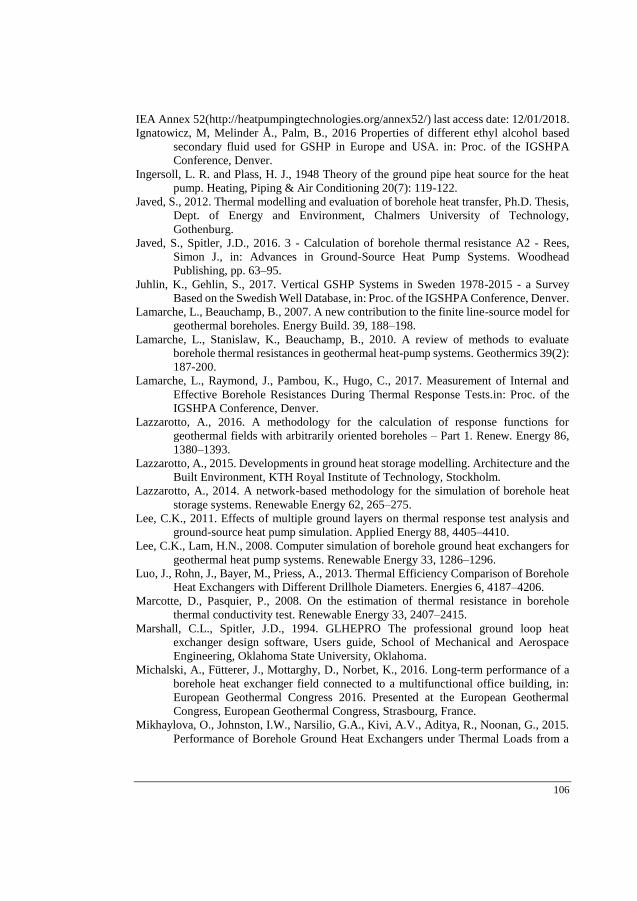
106
IEA Annex 52(http://heatpumpingtechnologies.org/annex52/) last access date: 12/01/2018.
Ignatowicz, M, Melinder Å., Palm, B., 2016 Properties of different ethyl alcohol based
secondary fluid used for GSHP in Europe and USA. in: Proc. of the IGSHPA
Conference, Denver.
Ingersoll, L. R. and Plass, H. J., 1948 Theory of the ground pipe heat source for the heat
pump. Heating, Piping & Air Conditioning 20(7): 119-122.
Javed, S., 2012. Thermal modelling and evaluation of borehole heat transfer, Ph.D. Thesis,
Dept. of Energy and Environment, Chalmers University of Technology,
Gothenburg.
Javed, S., Spitler, J.D., 2016. 3 - Calculation of borehole thermal resistance A2 - Rees,
Simon J., in: Advances in Ground-Source Heat Pump Systems. Woodhead
Publishing, pp. 63–95.
Juhlin, K., Gehlin, S., 2017. Vertical GSHP Systems in Sweden 1978-2015 - a Survey
Based on the Swedish Well Database, in: Proc. of the IGSHPA Conference, Denver.
Lamarche, L., Beauchamp, B., 2007. A new contribution to the finite line-source model for
geothermal boreholes. Energy Build. 39, 188–198.
Lamarche, L., Stanislaw, K., Beauchamp, B., 2010. A review of methods to evaluate
borehole thermal resistances in geothermal heat-pump systems. Geothermics 39(2):
187-200.
Lamarche, L., Raymond, J., Pambou, K., Hugo, C., 2017. Measurement of Internal and
Effective Borehole Resistances During Thermal Response Tests.in: Proc. of the
IGSHPA Conference, Denver.
Lazzarotto, A., 2016. A methodology for the calculation of response functions for
geothermal fields with arbitrarily oriented boreholes – Part 1. Renew. Energy 86,
1380–1393.
Lazzarotto, A., 2015. Developments in ground heat storage modelling. Architecture and the
Built Environment, KTH Royal Institute of Technology, Stockholm.
Lazzarotto, A., 2014. A network-based methodology for the simulation of borehole heat
storage systems. Renewable Energy 62, 265–275.
Lee, C.K., 2011. Effects of multiple ground layers on thermal response test analysis and
ground-source heat pump simulation. Applied Energy 88, 4405–4410.
Lee, C.K., Lam, H.N., 2008. Computer simulation of borehole ground heat exchangers for
geothermal heat pump systems. Renewable Energy 33, 1286–1296.
Luo, J., Rohn, J., Bayer, M., Priess, A., 2013. Thermal Efficiency Comparison of Borehole
Heat Exchangers with Different Drillhole Diameters. Energies 6, 4187–4206.
Marcotte, D., Pasquier, P., 2008. On the estimation of thermal resistance in borehole
thermal conductivity test. Renewable Energy 33, 2407–2415.
Marshall, C.L., Spitler, J.D., 1994. GLHEPRO The professional ground loop heat
exchanger design software, Users guide, School of Mechanical and Aerospace
Engineering, Oklahoma State University, Oklahoma.
Michalski, A., Fütterer, J., Mottarghy, D., Norbet, K., 2016. Long-term performance of a
borehole heat exchanger field connected to a multifunctional office building, in:
European Geothermal Congress 2016. Presented at the European Geothermal
Congress, European Geothermal Congress, Strasbourg, France.
Mikhaylova, O., Johnston, I.W., Narsilio, G.A., Kivi, A.V., Aditya, R., Noonan, G., 2015.
Performance of Borehole Ground Heat Exchangers under Thermal Loads from a
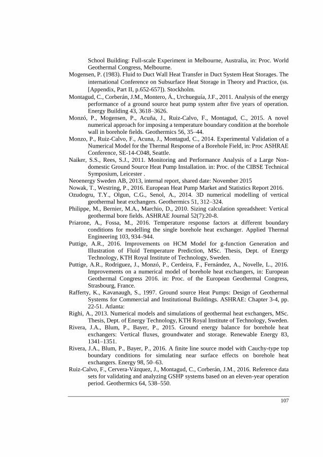
107
School Building: Full-scale Experiment in Melbourne, Australia, in: Proc. World
Geothermal Congress, Melbourne.
Mogensen, P. (1983). Fluid to Duct Wall Heat Transfer in Duct System Heat Storages. The
international Conference on Subsurface Heat Storage in Theory and Practice, (ss.
[Appendix, Part II, p.652-657]). Stockholm.
Montagud, C., Corberán, J.M., Montero, Á., Urchueguía, J.F., 2011. Analysis of the energy
performance of a ground source heat pump system after five years of operation.
Energy Building 43, 3618–3626.
Monzó, P., Mogensen, P., Acuña, J., Ruiz-Calvo, F., Montagud, C., 2015. A novel
numerical approach for imposing a temperature boundary condition at the borehole
wall in borehole fields. Geothermics 56, 35–44.
Monzo, P., Ruiz-Calvo, F., Acuna, J., Montagud, C., 2014. Experimental Validation of a
Numerical Model for the Thermal Response of a Borehole Field, in: Proc ASHRAE
Conference, SE-14-C048, Seattle.
Naiker, S.S., Rees, S.J., 2011. Monitoring and Performance Analysis of a Large Non-
domestic Ground Source Heat Pump Installation. in: Proc. of the CIBSE Technical
Symposium, Leicester .
Neoenergy Sweden AB, 2013, internal report, shared date: November 2015
Nowak, T., Westring, P., 2016. European Heat Pump Market and Statistics Report 2016.
Ozudogru, T.Y., Olgun, C.G., Senol, A., 2014. 3D numerical modelling of vertical
geothermal heat exchangers. Geothermics 51, 312–324.
Philippe, M., Bernier, M.A., Marchio, D., 2010. Sizing calculation spreadsheet: Vertical
geothermal bore fields. ASHRAE Journal 52(7):20-8.
Priarone, A., Fossa, M., 2016. Temperature response factors at different boundary
conditions for modelling the single borehole heat exchanger. Applied Thermal
Engineering 103, 934–944.
Puttige, A.R., 2016. Improvements on HCM Model for g-function Generation and
Illustration of Fluid Temperature Prediction, MSc. Thesis, Dept. of Energy
Technology, KTH Royal Institute of Technology, Sweden.
Puttige, A.R., Rodriguez, J., Monzó, P., Cerdeira, F., Fernández, A., Novelle, L., 2016.
Improvements on a numerical model of borehole heat exchangers, in: European
Geothermal Congress 2016. in: Proc. of the European Geothermal Congress,
Strasbourg, France.
Rafferty, K., Kavanaugh, S., 1997. Ground source Heat Pumps: Design of Geothermal
Systems for Commercial and Institutional Buildings. ASHRAE: Chapter 3-4, pp.
22-51. Atlanta:
Righi, A., 2013. Numerical models and simulations of geothermal heat exchangers, MSc.
Thesis, Dept. of Energy Technology, KTH Royal Institute of Technology, Sweden.
Rivera, J.A., Blum, P., Bayer, P., 2015. Ground energy balance for borehole heat
exchangers: Vertical fluxes, groundwater and storage. Renewable Energy 83,
1341–1351.
Rivera, J.A., Blum, P., Bayer, P., 2016. A finite line source model with Cauchy-type top
boundary conditions for simulating near surface effects on borehole heat
exchangers. Energy 98, 50–63.
Ruiz-Calvo, F., Cervera-Vázquez, J., Montagud, C., Corberán, J.M., 2016. Reference data
sets for validating and analyzing GSHP systems based on an eleven-year operation
period. Geothermics 64, 538–550.

108
Sakata, Y., Katsura, T., Nagano, K., Ishizuka, M.(2017) Field analysis of stepwise effective
thermal conductivity along a borehole heat exchanger under artificial conditions of
groundwater flow. Hydrology, 4 (2), 1-21 Spitler, J.D., Bernier, M., 2016. 2 - Vertical borehole ground heat exchanger design
methods A2- Rees, Simon J., in: Advances in Ground-Source Heat Pump Systems.
Woodhead Publishing, pp. 29–61.
Sundberg, J. 1991 Termiska egenskaper i jorg och berg. Swedish Geotechnical Institute,
Linköping, Sweden.
Sutton, M.G., Nutter, D.W., Couvillion, R.J., Davis, R.K., 2002. Comparison of multilayer
borefield design algorithm (MLBDA) to available GCHP benchmark data.
ASHRAE Trans. 108(1): 82-7.
Swedish Energy Agency (www.energimyndiheten.se), last access date: 14/06/2017
Tanaka, N., others, 2011. Technology roadmap: Energy-efficient Buildings: Heating and
Cooling Equipment. Int. Energy Agency Tech Rep.
Taylor, J.R. 1997. An introduction to error analysis, 2d ed. Sausalito: University Science
Books.
VINNOVA (www.vinnova.se), last access date: 15/06/2017
Witte, H.J., Van Gelder, G.J., Spitier, J.D., 2002. In situ measurement of ground thermal
conductivity: a Dutch perspective. ASHRAE Transactions 108 (1): 263-270.
Witte, H.J.L., 2013. Error analysis of thermal response tests. Applied Energy 109, 302–311.
Witte, H.J.L., 2016. 4 - In situ estimation of ground thermal properties A2 - Rees, Simon
J., in: Advances in Ground-Source Heat Pump Systems. Woodhead Publishing, pp.
97–116.
Yavuzturk, C., Spitler, J.D., 2001. Field validation of a short time step model for vertical
ground-loop heat exchangers ASHRAE Transactions 107 (1): 617-625.
Zeng, H., Diao, N., Fang, Z., 2003. Heat transfer analysis of boreholes in vertical ground
heat exchangers. Int. J. Heat Mass Transfer 46, 4467–4481.
Zeng, H.Y., Diao, N.R., Fang, Z.H., 2002. A finite line-source model for boreholes in
geothermal heat exchangers. Heat Transfer - Asian Research 31, 558–567.
doi:10.1002/htj.10057
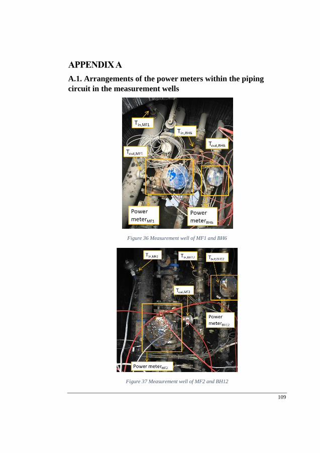
109
APPENDIX A
A.1. Arrangements of the power meters within the piping
circuit in the measurement wells
Figure 36 Measurement well of MF1 and BH6
Figure 37 Measurement well of MF2 and BH12
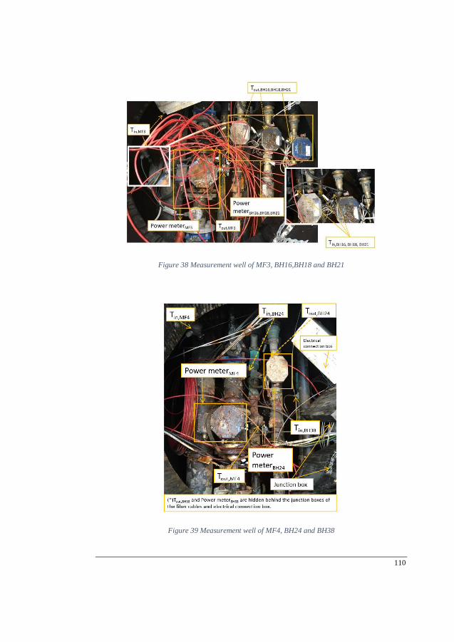
110
Figure 38 Measurement well of MF3, BH16,BH18 and BH21
Figure 39 Measurement well of MF4, BH24 and BH38
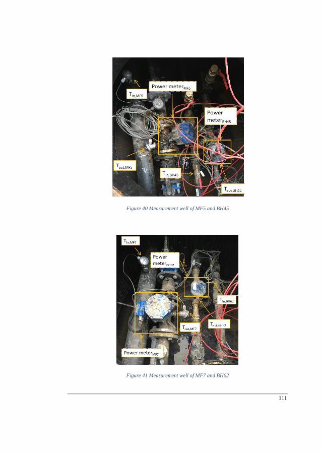
111
Figure 40 Measurement well of MF5 and BH45
Figure 41 Measurement well of MF7 and BH62
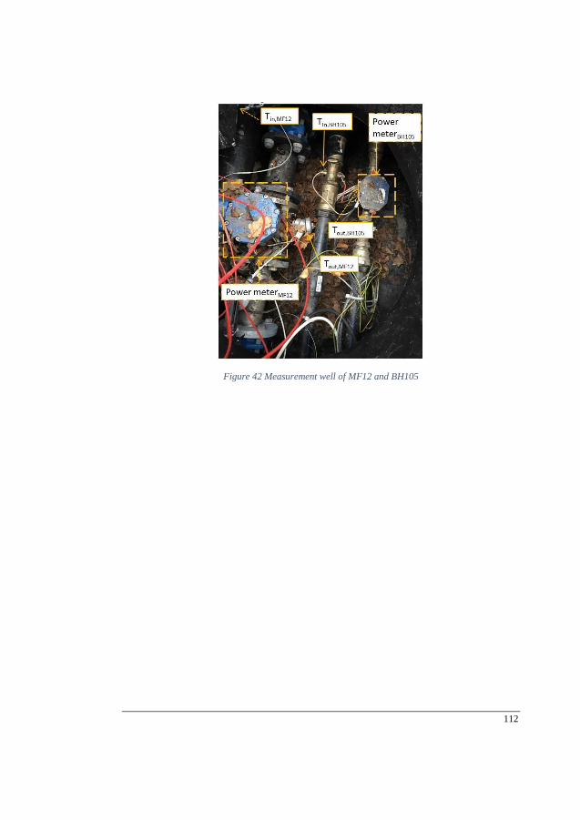
112
Figure 42 Measurement well of MF12 and BH105
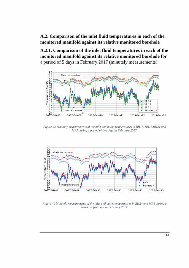
113
A.2. Comparison of the inlet fluid temperatures in each of the
monitored manifold against its relative monitored borehole
A.2.1. Comparison of the inlet fluid temperatures in each of the
monitored manifold against its relative monitored borehole for
a period of 5 days in February,2017 (minutely measurements)
Figure 43 Minutely measurements of the inlet and outlet temperatures in BH16, BH18,BH21 and MF3 during a period of five days in February 2017.
Figure 44 Minutely measurements of the inlet and outlet temperatures in BH24 and MF4 during a
period of five days in February 2017.
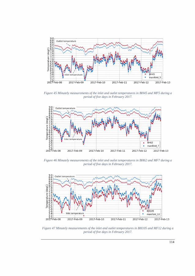
114
Figure 45 Minutely measurements of the inlet and outlet temperatures in BH45 and MF5 during a period of five days in February 2017.
Figure 46 Minutely measurements of the inlet and outlet temperatures in BH62 and MF7 during a
period of five days in February 2017.
Figure 47 Minutely measurements of the inlet and outlet temperatures in BH105 and MF12 during a period of five days in February 2017.
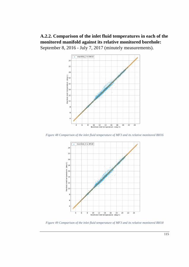
115
A.2.2. Comparison of the inlet fluid temperatures in each of the
monitored manifold against its relative monitored borehole:
September 8, 2016 - July 7, 2017 (minutely measurements).
Figure 48 Comparison of the inlet fluid temperature of MF3 and its relative monitored BH16
Figure 49 Comparison of the inlet fluid temperature of MF3 and its relative monitored BH18

116
Figure 50 Comparison of the inlet fluid temperature of MF3 and its relative monitored BH21
Figure 51 Comparison of the inlet fluid temperature of MF4 and its relative monitored BH24
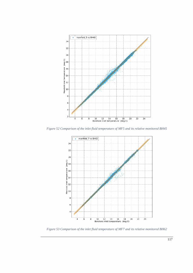
117
Figure 52 Comparison of the inlet fluid temperature of MF5 and its relative monitored BH45
Figure 53 Comparison of the inlet fluid temperature of MF7 and its relative monitored BH62
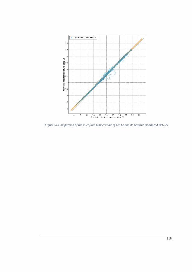
118
Figure 54 Comparison of the inlet fluid temperature of MF12 and its relative monitored BH105
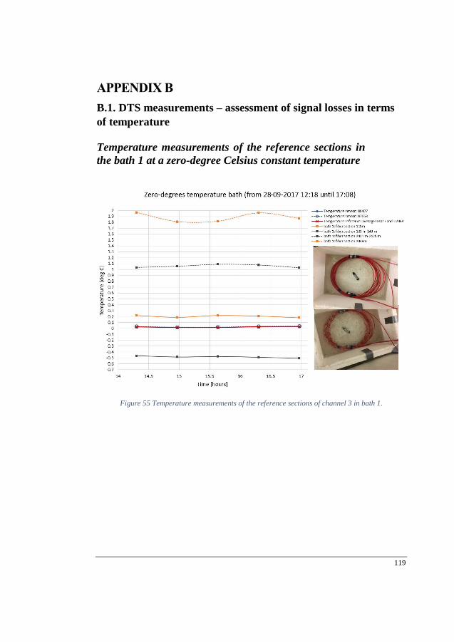
119
APPENDIX B
B.1. DTS measurements – assessment of signal losses in terms
of temperature
Temperature measurements of the reference sections in
the bath 1 at a zero-degree Celsius constant temperature
Figure 55 Temperature measurements of the reference sections of channel 3 in bath 1.
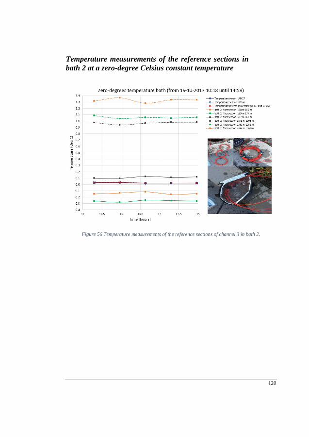
120
Temperature measurements of the reference sections in
bath 2 at a zero-degree Celsius constant temperature
Figure 56 Temperature measurements of the reference sections of channel 3 in bath 2.
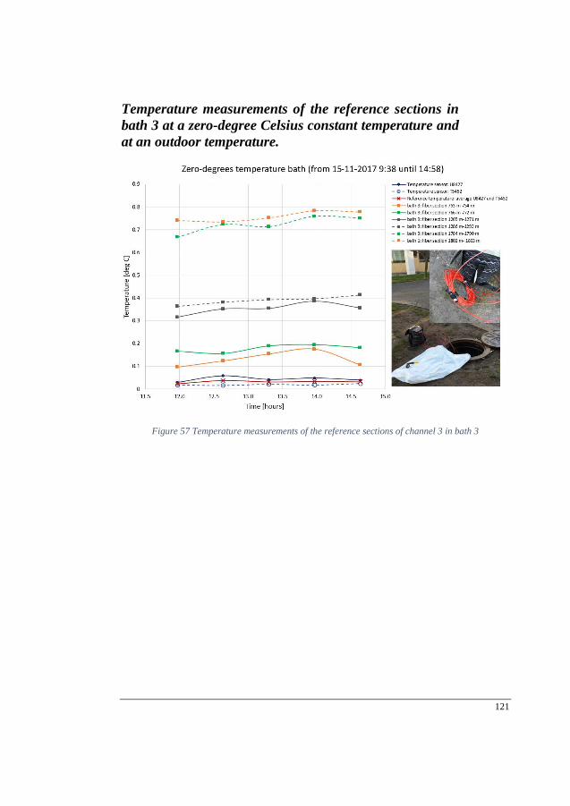
121
Temperature measurements of the reference sections in
bath 3 at a zero-degree Celsius constant temperature and
at an outdoor temperature.
Figure 57 Temperature measurements of the reference sections of channel 3 in bath 3
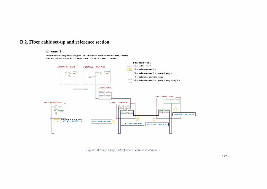
122
B.2. Fiber cable set-up and reference section
Figure 58 Fiber set-up and reference sections in channel 1
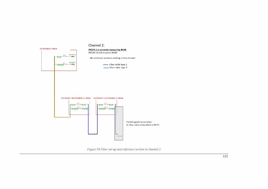
123
Figure 59 Fiber set-up and reference section in channel 2
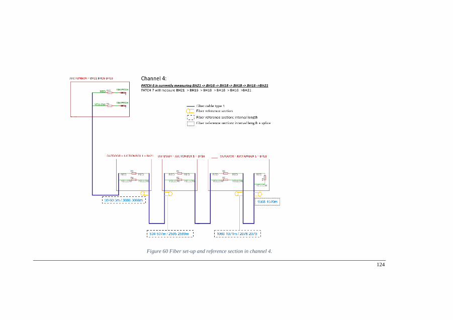
124
Figure 60 Fiber set-up and reference section in channel 4.