Fakulteit Ingenieurswese •

Faculty of Engineering

D epa r t e men t Me g an i e s e I n g en i e u r s we se • D ep a r t m e n t o f M e ch a n i c a l E n g i n ee r i n g

P r i v a a t S a k / P r i v a t e B a g X1 • M a t i e l a n d , 7 6 0 2 • S u i d - A f r i k a / S o u t h A f r i c a , T e l : +2 7 ( 0 ) 2 1 8 0 8 4 3 7 6 • F a k s / F a x : +2 7 ( 0 ) 2 1 8 0 8 4 9 5 8

Modelling and Design of a Novel Air-Spring for a Suspension Seat

Marco Wilfried Holtz

Fakulteit Ingenieurswese •

Faculty of Engineering

D epa r t e men t Me g an i e s e I n g en i e u r s we se • D ep a r t m e n t o f M e ch a n i c a l E n g i n ee r i n g

P r i v a a t S a k / P r i v a t e B a g X1 • M a t i e l a n d , 7 6 0 2 • S u i d - A f r i k a / S o u t h A f r i c a , T e l : +2 7 ( 0 ) 2 1 8 0 8 4 3 7 6 • F a k s / F a x : +2 7 ( 0 ) 2 1 8 0 8 4 9 5 8

Modelling and Design of a Novel Air-Spring for a Suspension Seat

Marco Wilfried Holtz

Thesis presented at the University of Stellenbosch in partial fulfilment of the requirements for the degree of

Master of Science in Engineering

Supervisor: Prof J.L. van Niekerk

December 2007

i

Declaration I, the undersigned, hereby declare that the work contained in this thesis is my own original work and that I have not previously in its entirety or part submitted it at any university for a degree.

Signature:…………………………… M.W. Holtz Date: 02 March 2008

ii

Abstract Suspension seats are commonly used for earth moving machinery to isolate vehicle operators from vibrations transmitted to the vehicle body. To provide the required stiffness and damping for these seats, air-springs are typically used in conjunction with dampers. However, to eliminate the need for additional dampers, air-springs can be used in conjunction with auxiliary air volumes to provide both spring stiffness and damping. The damping is introduced through the flow restriction connecting the two air volumes. In this study, simplified models of an air-spring were derived followed by a model including the addition of an auxiliary volume. Subsequent to simulations, tests were performed on an experimental apparatus to validate the models. The air-spring models were shown to predict the behaviour of the experimental apparatus. The air-spring and auxiliary volume model followed the trend predicted by literature but showed approximately 27 % lower transmissibility amplitude and 21 % lower system natural frequency than obtained by tests when using large flow restriction diameters. This inaccuracy was assumed to be introduced by the simplified mass transfer equations defining the flow restriction between air-spring and auxiliary volume. The models however showed correlation when the auxiliary volume size was decreased by two thirds of the volume actually used for the experiment. This design of a prototype air-spring and auxiliary volume is presented for a suspension seat used in articulated or rigid frame dump trucks. The goal of this study was to design a suspension seat for this application and to obtain a SEAT value below 1,1. The design was optimised by varying auxiliary volume size, flow diameter and load. A SEAT value of less than 0,9 was achieved.

iii

Uittreksel Suspensie sitplekke word dikwels in grondverskuiwingsvoertuie gebruik om bestuurders te isoleer van die vibrasies wat vanaf die voertuig se onderstel oorgedra word. Om die nodige styfheid en demping vir hierdie sitplekke te voorsien, word daar normaalweg lug-vere te same met dempers gebruik. Om die noodsaaklikheid van ekstra dempers uit te skakel, word lugvere met eksterne lug volumes gebruik om die veer met addisionele demping te voorsien. Die demping word verskaf deur die vloeiweerstand wat hierdie twee lug volumes met mekaar verbind. In hierdie studie is drie modelle vir ´n lug-veer afgelei. Dit is gevolg deur die afleiding van ´n model waar die eksterne volume bygevoeg is. Die simulasies is gevolg deur toetse op ´n eksperimentele opstelling om die modelle te bekragtig. Die lug-veer modelle het die gedrag van die eksperimentele opstelling voorspel. Die lug-veer en eksterne volume model het die tendense wat in literatuur voorspel is weergegee. Die oordraagbaarheidsamplitude was 27% laer en die natuurlike frekwensie 21% laer wanneer groot deursnee vloeiweerstande by toetse gebruik is. Dit word aangeneem dat hierdie onnoukeurigheid deur die vereenvoudigde massa oordrags vergelykings, wat die vloei weerstand tussen die lug veer en die eksterne volume beskryf, veroorsaak word. Die modelle het vergelykbare resultate gelewer, as die eksterne volume met twee derdes verminder is. Die ontwerp van ´n prototipe lug-veer met ‘n eksterne volume is ontwikkel vir ´n suspensie sitplek wat vir stortvragmotors gebruik word. Die doel van die studie was om ´n suspensie sitplek vir hierdie doel te ontwerp en ´n SEAT waarde van minder as 1,1 te verkry. Die ontwerp is geoptimiseer deur middel van die eksterne volume grootte, die vloei weerstand deursnee en die las te verander. ´n SEAT waarde van minder as 0,9 is uiteindelik verkry.

iv

Dedicated to my parents for their unwavering support

v

Acknowledgements I would like to extend a thank you to Professor J. L. van Niekerk for his supervision and securing finances for the duration of my thesis. These have been critical in making the project possible. Further thanks are to Ferdi Zietsman, Graham Hamerse, Anton van den Berg and Calvin Hamerse for the manufacturing of components for the experimental setup and Cobus Zietsman for providing the components and materials for the air system. Your advice in these matters has also been valuable.

vi

Table of contents 1. Introduction......................................................................................................1

1.1. Whole body vibrations.............................................................................2

1.2. Suspension seats and air-springs..............................................................4

1.3. Objectives and scope ...............................................................................7

1.4. Thesis overview .......................................................................................8

2. Literature survey ............................................................................................10

2.1. Air-springs .............................................................................................10

2.2. Modelling...............................................................................................13

3. Modelling.......................................................................................................16

3.1. Linear spring model ...............................................................................16

3.2. Non-linear spring model ........................................................................19

3.3. Complex non-linear spring model .........................................................21

3.4. Air-spring model with auxiliary volume ...............................................22

4. Experiment.....................................................................................................27

4.1. Experimental apparatus..........................................................................27

4.2. Test equipment and procedures .............................................................30

5. Results – simulation and testing ....................................................................34

5.1. Air-spring simulation and experiment results........................................34

5.2. Auxiliary volume simulation and experiment results ............................37

5.3. Discussion of simulation and experiment results ..................................41

6. Procedure to design novel air-spring suspension...........................................42

6.1. Design parameters and criteria ..............................................................42

6.2. Design procedure and simulation ..........................................................46

7. Conclusion and recommendations .................................................................51

8. References......................................................................................................53

Appendix A: Derivations of state equations............................................... A - 1

A.1 Linear spring model .......................................................................... A - 1

A.2 Non-linear spring model ................................................................... A - 4

A.3 Complex non-linear spring model .................................................... A - 5

vii

A.4 Air-spring model with auxiliary volume .......................................... A - 7

A.5 Simulation parameters .................................................................... A - 14

Appendix B: List of instrumentation and test settings ................................B - 1

Appendix C: Results....................................................................................C - 1

C.1 Air-spring simulation and test – load case 1, 1 - 3m/s2 r.m.s...........C - 1

C.2 Air-spring simulation and test – load case 2, 1 - 3m/s2 r.m.s. .........C - 4

C.3 Air-spring simulation and test – load case 3, 1 - 3m/s2 r.m.s...........C - 7

C.4 Air-spring simulation and test – load case 4, 1 - 3m/s2 r.m.s.........C - 10

C.5 Air-spring and auxiliary volume simulation and test – load case 1, 1 -

3m/s2 r.m.s....................................................................................................C - 13

C.6 Air-spring and auxiliary volume simulation and test – load case 3, 1 -

3m/s2 r.m.s....................................................................................................C - 16

viii

List of tables Table 3.1: Equivalent spring stiffness model state equations................................18

Table 3.2: State equations of non-linear spring model ..........................................20

Table 3.3: State equations of complex non-linear spring model ...........................21

Table 3.4: State equations of complex spring model with auxiliary volume ........25

Table 4.1: Experimental apparatus parameters......................................................29

Table 4.2: Settings used for simulations and test runs...........................................32

Table 6.1: SEAT values for various load cases .....................................................48

Table A.1: Equivalent spring stiffness model state equations……………...…A - 4

Table A.2: State equations of non-linear spring model……………………….A - 5

Table A.3: State equations of complex non-linear spring model…………..…A - 7

Table A.4: State equations of complex spring model with auxiliary volume..A - 13

Table A.5: Simulation parameters…………………………………………….A - 1

Table B.1: Numbers designated for results files of test runs………………….B - 1

Table B.2: List of test equipment…………………………………………...…B - 1

Table B.3: Settings on .vna file – MC Setup…………………………………..B - 2

Table B.4: Example of test sheet to document testing……………………..….B - 2

ix

List of figures Figure 1.1: Frequency range and magnitude for human vibration – (Mansfield,

2005) ........................................................................................................................3

Figure 1.2: Basicentric vibration axes in seated position – (ISO 2631, 1997) ........4

Figure 1.3: Transmissibility of rigid, foam and metal sprung and suspension seats

– (Griffin, 1990).......................................................................................................5

Figure 1.4: Convoluted air-spring (left-hand side) and reversible sleeve air-spring

(right-hand side) – (Firestone) .................................................................................7

Figure 1.5: Flow chart of project .............................................................................9

Figure 2.1: Air suspension layout - air-spring and auxiliary volume with resistance

– (Quaglia and Sorli, 2001)....................................................................................11

Figure 2.2: Frequency response of non-linear air-spring model with varying

conductance – (Quaglia and Sorli, 2001)...............................................................12

Figure 3.1: Spring model and free body diagram ..................................................17

Figure 3.2: Sketch of air-spring with sectioned views...........................................18

Figure 3.3: SIMULINK block diagram of linear spring model .............................19

Figure 3.4: SIMULINK block diagram of non-linear spring model......................20

Figure 3.5: SIMULINK block diagram for complex non-linear spring model

including boundary work .......................................................................................22

Figure 3.6: Model of spring with auxiliary volume and free body diagram..........23

Figure 3.7: SIMULINK block diagram of spring and auxiliary volume model ....26

Figure 4.1: Sketch of experimental apparatus .......................................................27

Figure 4.2: Air supply to spring and flow connector between air-spring and

auxiliary volume (top), and configuration of connector (bottom) .........................28

Figure 4.3: Experimental apparatus on servo actuated hydraulic platform ...........29

Figure 4.4: Data processing and control equipment ..............................................30

Figure 4.5: Pressure gauge and shut off valves .....................................................31

Figure 4.6: Transmissibility curve for air-spring experiment at load case three ...33

Figure 5.1: Comparison of transmissibility for air spring models at load case three

...............................................................................................................................35

x

Figure 5.2: Comparison between transmissibility for air spring models and

experimental apparatus at load case three..............................................................36

Figure 5.3: Transmissibility curves of spring auxiliary volume model .................37

Figure 5.4: Transmissibility curves of experiment with air-spring .......................39

Figure 5.5: Transmissibility curves of air-spring and auxiliary volume................40

Figure 5.6: Transmissibility curves of air-spring and auxiliary volume................40

Figure 6.1: The effects of changing flow restriction diameter ..............................43

Figure 6.2: PSD plot and r.m.s. value for spectral class EM1 – ISO 7096............44

Figure 6.3: Weighting function Wk for WBV in the z-direction – ISO 2631:1 ....45

Figure 6.4: System response with increasing flow restriction diameter ................47

Figure 6.5: System response with increased auxiliary volume size ......................47

Figure 6.6: System response with increasing flow restriction diameter ................49

Figure 6.7: Air-spring and auxiliary volume effectiveness ...................................49

Figure A.1: Spring model and free body diagram………………………….....A - 1

Figure A.2: Sketch of air-spring with sectioned views and illustration of spring

effective area, A1…………………………………..…………………………..A - 3

Figure A.3: Model of spring with auxiliary volume and free body diagram….A - 8

xi

Nomenclature The subscripts ‘1’ and ‘2’ used in the text and equations refer to the air-spring and auxiliary volume respectively. The subscript ‘0’ refers to reference or equilibrium conditions. No numerical subscript indicates a constant value. A Area As Heat transfer area Cν,av Averaged specific heat between T1 and T2 for constant volume process Cν Specific heat for constant volume process c Damping constant D1 Air-spring inner diameter D2 Air-spring outer diameter d Flow restriction diameter e Wall roughness E Energy F Force f Applied force(s) in equation of motion floss Friction factor g Gravitational acceleration hQ Heat transfer coefficient hL Pressure loss h Height of spring henth Enthalpy h& Velocity of deflected point of spring h&& Acceleration of deflected point of spring Δh Deflection of spring from equilibrium position KE Expansion loss coefficient KC Contraction loss coefficient kequ Equivalent spring constant l Flow restriction length mload Suspended mass m Air mass n Ratio of specific heats/constant for polytropic process Pa Atmospheric pressure Pr Relative pressure P Internal pressure ΔP Pressure differential Q Heat transfer ΔQ Change in heat transfer Q& Rate of heat transfer R Gas constant Ts Temperature of heat transfer surface Tr Relative temperature

xii

T Temperature ΔT Change in temperature T& Rate of temperature change Δt Time increment U Internal energy ΔU Change in internal energy V Volume W Work done ΔW Change in work ωn System natural frequency y Total/absolute piston displacement y& Total piston velocity y&& Total piston acceleration z Spring base displacement z& Spring base velocity z&& Spring base acceleration γ Specific weight ζ Damping ratio

1

1. Introduction Vibrations are encountered by any vehicle as it is driven over an irregular road surface. As a result, it is customary for vehicles to be fitted with suspension systems to reduce the vibrations transmitted to the vehicle body and its occupants. Furthermore, as greater loading capacities have been developed, and vehicles are able to travel at higher speeds, stiffer suspensions are designed, resulting in larger vibration inputs to the vehicle. These design measures to improve productivity have resulted in both the vehicle body and the human occupants being subjected to higher levels of vibration. The consequences of these increased vibrations are both fatigue and injury to the humans, and damage to the machinery. Vehicle operators, in particular, suffer from fatigue and resultant injuries from continuous exposure to vibration, specifically in the mining, construction and haulage sectors where they are subjected to vibrations for extended periods of time. In attempting to reduce these problems, particular attention has been focused on reducing vibrations transmitted to the operator by isolating the vehicle operator from the vibrations of the vehicle. This was accomplished by adding seat suspensions to vehicles, as seats are the final area where vehicle vibration can be isolated from the operator. Vehicle suspensions are incapable of preventing the transmission of continuous vibration and large amplitude or shock excitations to the operator, so the addition of seat suspensions aims to reduce this vibration transmission before it is perceived by the operator. Over the last forty years, air-springs have been used more in suspension systems, initially in the agriculture, transport and freight sectors, and in the last twenty years, they have been used increasingly so in the commercial and private vehicle sectors. Air-spring technology is the preferred technology used in suspension seats owing to its advantages over conventional mechanical coil suspension systems. These advantages include:

● Varying spring rates determined by the internal pressure and excitation force, and frequency of the vibration (Kornhausser, 1994)

● Easy to maintain correct suspension height around the ‘design point’ by adjusting the spring pressure as the load is varied

● Light weight ● Good vibration isolation properties

Conventional suspension systems use coil springs in conjunction with hydraulic dampers to achieve the desired stiffness and damping for their design application. In contrast to these systems, certain air suspensions use flexible re-enforced rubber bellows or a rolling diaphragm connected to an auxiliary air volume

2

reservoir by a flow restriction. The flow restriction introduces damping, whilst the compressed air determines the stiffness of the springs. It therefore becomes a single device that provides the function of two traditionally separate entities whilst keeping /maintaining all the benefits of air springs. One problem is that air-springs are difficult to model in comparison to the traditional coil springs. This can be attributed to the fact that a gas is used as the component providing the stiffness, thereby introducing thermodynamic effects. When an auxiliary volume is added to the air spring, further thermodynamic and fluid mechanic effects are introduced, due to mass transfer between the two air volumes. In order to design and develop prototype air-springs, the device requires accurate modelling. Thus an air-spring and auxiliary volume model needs to be generated as a means to develop a prototype. The interest in this project lies in developing such an air-spring with auxiliary volume model that is used for a suspension seat in articulated or rigid frame dump trucks, using the EM1 spectral class as defined in ISO 7096 (2000). The remainder of this introductory chapter presents some background on whole body vibration and suspension seats and briefly highlights air-springs that are now widely used in this type of seat. The objectives and scope of this research project are discussed and the chapter is concluded with an overview of the remaining paper.

1.1. Whole body vibrations Vehicle operators are exposed to what is known as whole-body vibrations (WBV). These vibrations can vary in magnitude and frequency. The continuous prolonged exposure to vibrations as well as instances of impact loadings can result in excessively large forces being transmitted to the driver. This can cause driver discomfort and physiological damage. Human response to WBV as explained by Griffin (1990) is typically threefold: degraded comfort, interference with activities and impaired health. The factors determining the type and extent of effect are the frequency, direction and magnitude of the vibrations, as well as the duration of WBV exposure. The frequencies transmitted by seats are predominantly below 20 Hz, with somewhat higher frequencies transmitted by the vehicle floor (Griffin, 1990). As illustrated in Figure 1.1, Mansfield (2005) found WBV can be seen to take effect in this region of approximately 1 Hz to 20 Hz. Below 1 Hz, motion sickness is prevalent. For seated subjects, sensitivity to vertical vibration occurs in the frequency range between 2 to 3 Hz and 5 to 6 Hz (Griffin, 1990).

3

Figure 1.1: Frequency range and magnitude for human vibration – (Mansfield,

2005) The general range of interest for vibration magnitudes is from about 0.01 m/s2 to 10.0 m/s2. Below 1 Hz and above 20 Hz, higher vibrational magnitudes than 0.01 m/s2 are required for humans to detect vibrations. WBV with magnitudes of 10.0 m/s2 r.m.s. and higher are considered hazardous (Griffin, 1990). Typical vibrations experienced in off-road vehicles are at low frequencies between 1 Hz and 10 Hz and high amplitudes of about 1.5 m/s2. These can cause or aggravate physical symptoms that impair driver health in predominantly two major areas: gastric complaints and spinal disorders (Ishitake et al, 2001, Pope et al, 1998, Pope and Hansson, 1992). To determine the vibrations that are transmitted to test subjects or occupants, certain guidelines need to be followed during testing to ensure they are measured correctly. Standards have been drawn up to provide these guidelines, of which ISO 2631-1 (1997) is an example, dealing with the evaluation of human exposure to whole-body vibrations. To ascertain the direction of vibration, the human body is given a number of axes along which the vibration can be measured. This enables the accurate definition of vibration direction and forms the base for the experimental set-up when measuring the vibrations. The ISO 2631 standard part 1 (1997) for mechanical vibration and shock provides the direction of the axes as depicted in Figure 1.2. The frequency range covered by the standard is from 0.1 Hz to 80 Hz and provides guidance on the possible effects of vibration on health, comfort, perception of vibration and motion sickness. This standard deals specifically with vibrations transmitted to the human body as a whole through the supporting surfaces.

4

Figure 1.2: Basicentric vibration axes in seated position – (ISO 2631, 1997)

As indicated in the preceding section, suspension seats provide the final means of isolating vehicle occupants from vibration. Used in conjunction with air-springs, they provide an effective means of reducing vibrations transmitted to vehicle occupants, and are discussed further in the following section.

1.2. Suspension seats and air-springs Suspensions have been introduced in cab and seat design to reduce the exposure to vibrations, in the light of driver performance and health and safety. The need for cab and seat suspensions became more important as labour health costs increased, along with stricter requirements for operator safety, and the performance capabilities of machinery increased leading to greater vibrations, particularly in agricultural vehicles such as tractors not equipped with wheel suspensions (Hostens and Ramon, 2003). The same is also applicable to marine craft and suspended vehicles like trucks, busses and mining machinery. Seat suspensions then become of particular interest to improve operator comfort. They need to be optimised to reduce the transmitted vibrations and developing new seats is done by first generating models of the seats and their human occupant, and seeing the results of various testing regiments. A number of models have been created, ranging from very basic to

5

more complex. The basic models represent the suspension seat by a simple spring and damper and the occupant’s sprung mass is modelled as an effective mass. The more complex models incorporate end stop buffers and the human as a system of lumped masses with spring and damping characteristics (Kim et al, 2003). When looking at seat comfort, both static properties and dynamic properties can be considered. Particularly the dynamic behaviour becomes important when designing an optimum seat for vehicles. An optimum seat would be one that attenuates unwanted vibrations, preventing or minimising their transmission but still be cost effective in achieving this. To determine the transmission of vibrations by a seat, the accelerations are measured and compared at the seat mounting on the floor, and the interface between the seat and seated person. Guidelines for testing suspension seats are provided by ISO 7096 (2003). In accordance with ISO 10326-1 (1992), this standard specifies the laboratory method for the measurement and evaluation of seat suspension effectiveness to reduce WBV transmitted to operators of earth-moving machines at frequencies between 1 and 20 Hz. During testing, transmissibility may be affected by whether a person is used to test the seat or simply an equivalent mass as a rigid mass could over exaggerate the amplification. This can be attributed to the lack of damping - a human occupant provides damping due to his or her physiological properties. Various seat transmissibilities are illustrated in Figure 1.3 taken from Griffin.

Figure 1.3: Transmissibility of rigid, foam and metal sprung and suspension seats –

(Griffin, 1990)

6

Transmissibility of conventional seats is generally quite high at around 4 Hz with attenuation from 6 Hz upwards. Suspension seats show much lower amplification, occurring at about 2 Hz and attenuation occurring at about 3 to 4 Hz as illustrated in Figure 1.3 (Griffin, 1990). The seat effective amplitude transmissibility or ‘SEAT’ value is a method of communicating the dynamic performance of the seat, as it factors in the vibration spectrum, seat transmissibility and human response to vibrations (Griffin, 1990). A SEAT value of greater than 100% indicates the seat amplifies the vibration and if the value is below 100%, the seat’s dynamic behaviour has reduced the vibrations transmitted from the floor. For high vibration levels and at frequencies to which the human body is most sensitive, the attenuation needs to be the highest, and at frequencies where the human body is least sensitive, little or no attenuation is required. The SEAT value thus provides a measure combining these relevant factors. The SEAT value is defined as

100% ×××

=WeightingFlooronVibration

WeightingSeatonVibrationSEAT (1.1)

It can be calculated by the expression

100)()(

)()(%

2/1

2

2

×⎥⎥

⎦

⎤

⎢⎢

⎣

⎡=∫∫

dffWfG

dffWfGSEAT

iff

iss (1.2)

where Gss(f) and Gff(f) are the seat and floor acceleration power spectra, and Wi(f) is the frequency weighting for the human response to vibration which is of interest (Griffin, 1990). It is important to note the vibration weighting refers to the vibration occurring on the seat. To attenuate vibrations transmitted to the occupant, suspension seats have generally used the conventional coil spring and hydraulic damper combination. To further improve on these suspensions, air-spring technology, initially being used in vehicle suspensions, was introduced. The reasons for the increased popularity of air-springs compared to the conventional coil spring and damper suspensions as presented in Quaglia and Sorli (2001) are their

• adjustable carrying capacity, • reduced weight, • variable spring rate with constant ‘tuned’ frequency, • reduced structurally transmitted noise, and • variable ride height.

7

There are two main types of air-springs: bellows, also known as convoluted air-springs, and rolling diaphragm springs, also called reversible sleeve springs. These two types of springs are illustrated in Figure 1.4, both illustrations are taken from Firestone. Each type of spring is more suited to certain applications and exhibits different stiffness characteristics due to geometry and material composition. There are numerous sizes and configurations available for each type.

Figure 1.4: Convoluted air-spring (left-hand side) and reversible sleeve air-spring (right-hand side) – (Firestone)

Various suspension seats have been developed. However most work in modelling suspension seats focussed on the behaviour of the occupant in conjunction with a conventional suspension system using coil springs and hydraulic dampers. The area of interest for this project lies in modelling the air-spring with an auxiliary volume, thereby replacing the conventional components of the suspension seat.

1.3. Objectives and scope The objective of this project was the development of a model of a suspension system for a seat, comprising of an air-spring with an auxiliary volume. It required analytical modelling of the system and simulation of its dynamic response. The accuracy of the model was verified by testing an air-spring on a test rig. This enabled simulation in a controlled environment. Subsequent to the verification of the model, it was used to design a new suspension system that can in future be tuned further for certain excitation and loading conditions as experienced by typical earth moving equipment.

8

The objectives for the project are summarised below: • develop an accurate simulation model of an air-spring incorporating non-

linear characteristics such as fluid dynamic and thermodynamic effects • verify the simulation model by experimental testing • design a prototype air-spring for a suspension seat • test prototype model by running simulations

The resistive element in the air-spring is generally represented either by a pipe with varying diameter or an orifice, the diameter of which can be varied. The modelling of the pipe and the air mass inside it however can be somewhat cumbersome and the dynamic behaviour undesirable due to the inertia effects of the air mass in the pipe. The aim of the project was to develop a model and prototype that does not have a long pipe as a connection between the two air volumes but a shorter connection. This could be a resistive device in the form of an orifice or short pipe section directly connecting the two air chambers. This type of configuration has been previously used for vehicle suspensions and railway wagon secondary suspensions. However, the novelty of this air-spring configuration lies in that it has never been used before for the application of seat suspensions. The project thus incorporates design and development of a new air suspension consisting of an air-spring with an auxiliary volume. This system was refined to improve its attenuation of different input frequencies, depending on the field of application.

1.4. Thesis overview More detail of the work done for this project and a brief outline of each chapter is now presented. In Chapter 2, the literature survey reviews the two main components of this project namely air-springs and their modelling. A few papers are discussed to provide some background information on the topic. In Chapter 3, three different models for the air-spring are derived and presented, ranging from a linear spring model to a complex non-linear model. This chapter also presents the derivation of the air-spring and auxiliary volume model that is used to develop the simulation of the prototype. Figure 1.5 presents a flow chart of the procedure followed in developing the spring models through to the design of the prototype. The experimental apparatus and testing procedures are presented in Chapter 4. Here the physical testing is performed on an air-spring, as well as testing of the air-spring and auxiliary volume combination. The results of both experimental and numerical simulations are presented Chapter 5.

9

Chapter 6 deals with the procedure to design a prototype air spring. Firstly the main parameters in the design envelope that influence the response are presented. Based on these parameters, the prototype is developed by taking into consideration specifications presented in the ISO 7096 standard. The final chapter, Chapter 7, presents the conclusions and gives some recommendations for further work.

Figure 1.5: Flow chart of project

Modelling

Simulation

Satisfactory

Testing

Satisfactory

Prototype Design

Satisfactory

Project Completed

Yes

Yes

Yes

No

No

No

Simulation

Change Parameters

Change Parameters

10

2. Literature survey It is difficult to design and model air suspension systems. Despite similarities to the force-distance relationship of conventional mechanical springs, this relationship in air-springs is more complex. This is due to non-linearity brought

about by spring geometry and ‘complex interaction of heat transfer, fluid mechanics and thermodynamics’ (Kornhauser, 1994). The air-spring model needs to be accurate and yield accurate simulation results comparable to those obtained through experimental tests. Due to this non-linearity, the governing equations of the model need to incorporate equations of heat transfer, fluid dynamics and thermodynamics. Furthermore, the model needs to be generated in a computational environment that will be capable of managing the complexities and requirements to simulate the system.

2.1. Air-springs Air-springs have found wide application in the commercial sectors of earth-moving equipment, transportation and haulage, particularly in the heavy vehicle sectors where construction vehicles, mining equipment, trucks, busses and trains have been equipped with such suspensions. Air suspensions are also used in suspension seats and have proven themselves ideally suited for this application. As increased importance is placed on driver seat comfort, health and safety, vibration isolation has seen further advances by means of active or semi-active systems. These too have found wide application, particularly in the luxury vehicle sector where they enable suspension adjustment to road conditions or driver preference. Semi-active systems however come at a high cost due to the complexity required for such sophisticated sensory and control mechanisms, required to continually sense and regulate the suspension. Passive systems, despite their lack of direct feedback control, still provide a viable cost effective and far less complex alternative. They can be designed and adjusted for specific applications and still provide the advantages offered by air-springs mentioned in chapter 1. When using air-springs in suspension systems, they predominantly exhibit stiffness and, as with conventional coil springs, require additional damping. In the air-spring, the pressurised air inside the flexible mounting acts as the spring force, working against the applied load. The air-spring does provide some damping due to flexing and friction of the rubber-chord material. However to eliminate the need for an additional hydraulic damper, air-springs have been used in conjunction with auxiliary volumes (Quaglia and Sorli, 2001).

11

In most instances, these systems are made up of the bellows or diaphragm air-spring connected to an auxiliary reservoir by a thin tube offering resistance to the flow of air. Such a system is depicted in Figure 2.1 taken from Quaglia and Sorli (2001), and is an instance of a vehicular suspension. The interaction between these two air volumes and the resistance between them determines the dynamic characteristics of the system, the gas or air-spring and auxiliary volume determine the stiffness of the system, and the resistance, to the greatest part, the damping of the system. Through this resistance, damping is introduced into the system to eliminate the need for additional hydraulic dampers.

Figure 2.1: Air suspension layout - air-spring and auxiliary volume with resistance – (Quaglia and Sorli, 2001)

For the air-spring, the change in spring stiffness can be attributed to two main factors: the change in the pressure of the spring, and its effective area, which is attributed to the flexibility of the bellow or diaphragm. The spring stiffness is determined by the force applied to the spring and the internal pressure. These can be used in the simple equation of force equals pressure times area to calculate the effective area. This effective area is generally determined experimentally by applying a static force to the spring and measuring the internal or gauge pressure at that position, from which the effective area can be calculated. Change in volume, and therefore pressure, can be seen as static as well as dynamic. Deflecting the spring statically causes a change in its geometry. Similarly to its area change, the volume will also change as a result. In the case of dynamic changes in volume, simulations have indicated that for higher frequencies, the stiffness and behaviour of the spring is determined in effect only by its own volume. The resistive connection between the air volumes acts as a constriction, preventing air passing through it due to the spring’s rapid oscillation. For lower frequencies, the spring’s stiffness is determined by both its own volume and that of the auxiliary chamber. In this instance, the air is allowed to pass through the resistive connection (Quaglia and Sorli, 2001).

12

Furthermore the dynamics of the system are also influenced by the nature of the excitation, more specifically the excitation frequency and amplitude. The stiffness of the spring varies with a change in frequency. The frequency response of the system tends to show a change of magnitude in the transmitted vibration. This is linked to the effect of the interaction between the spring volume and auxiliary volume depending on the resistance connecting the two. When plotting this on a graph as shown in Figure 2.2, there is a common point for all the curves located between the maximum peaks of transmissibility: one for the spring stiffness due to its own volume, fS, and the other due to the combined volumes, fSV. For a specific resistance, the peak shifts to this common point which is lower than the two maxima, point ‘B’. The aim is thus to find the correct resistance or, inversely, conductance value for the specific spring/auxiliary volume ratio, placing the peak at the lowest point to ensure the lowest transmissibility (Quaglia and Sorli, 2001).

Figure 2.2: Frequency response of non-linear air-spring model with varying conductance – (Quaglia and Sorli, 2001)

This alone does not guarantee ideal suspension behaviour. Step response analyses suggest that excitation amplitude effect response characteristics as well. For large amplitude step inputs, a small conductance, or small value for the parameter C in Figure 2.2, the graph will show a large initial peak and modest attenuation. A larger conductance shows a lower initial peak and improved attenuation; however, the smaller oscillations last for longer. For a smaller step input, an intermediate

13

value showed the best attenuation for the initial oscillations. From this behaviour it was concluded that conductance should increase with an increase in the pressure (Quaglia and Sorli, 2001). The above discussion illustrates that the spring requires correct design to prevent increased or excessive transmission in the vicinity of the resonance frequency, taking into account its field of application and desired response. This would require design for operation under either constant vibration input or shock input. Some applications however might require striking a balance between design for frequency response and shock input. There are also thermodynamic, fluid mechanic and heat transfer considerations governing the spring behaviour. This is due to the compression and expansion of the pressurised gas and the gas flow inside and in-between the spring volume and auxiliary volume. To satisfy the laws of thermodynamics, the continuity, momentum and energy equations need to be derived for the system as presented by Toyofuku et al (1999) and Quaglia and Sorli (2001). Thus each of the volumes in the model and the resistance are defined by these equations. The model then incorporates each of these components to accurately represent the air-spring. These factors create non-linearities which make the modelling more complex compared to the conventional mechanical springs. Many suspension seat models focus on the behaviour of the occupant and the conventional suspension system using coil springs and hydraulic dampers. The area of interest for this project is the use of air-springs and an auxiliary volume as a substitute for the conventional components. The focus is placed on generating an accurate model of the actual air-spring; however, accurately modelling the behaviour provides numerous challenges.

2.2. Modelling Various methods have been devised to generate models that will accurately determine the response of springs to different input excitation frequencies and magnitudes. Improvement has been made in the accuracy of the spring models by incorporating the thermodynamic, heat transfer and fluid mechanic components in the models (Kornhauser, 1994). Qauglia and Sorli (2000) derive the stiffness of their air-spring model based on the basic force-distance relationship. Considering that the force can be attributed to the air pressure inside the spring and the area this pressure acts on, spring stiffness is defined as a function of pressure and spring area. As the spring pressure and area change continuously during spring compression or expansion, the differential form is used for each of these. The spring stiffness is thus divided

14

into essentially two parts: the stiffness due to the change in volume – this gives rise to the change in pressure, and the stiffness due to the area change. Expanding on this work, Quaglia and Sorli included an auxiliary volume (2001). This necessitated the introduction of a continuity equation to account for mass flow between the air-spring and auxiliary volume. In addition to this, the flow-restriction between these two volumes was characterised by using mass flow rate equations provided by ISO 6358. This international standard presents the method to characterise flow restrictions by means of experiment using specific test equipment to obtain conductance values used in the mass flow rate equations. Using these flow equations, Quaglia and Sorli then obtained different transmissibility magnitudes and resonant frequencies by changing the conductance or resistance between the air-spring and auxiliary volume. This method allowed tuning the suspension to yield an optimum point with low transmissibility characteristics. Another area for which air-springs and auxiliary volumes are modelled is pneumatic vibrations isolators. In these devices, the air-spring assumes more of a piston configuration. The air-spring is connected to the auxiliary volume, typically called a damping chamber, by means of a capillary tube. A number of papers and books discuss modelling of pneumatic vibration isolators. Here the equations defining the mass flow rate are for capillary tubes with laminar flow and small variations between upstream and downstream pressures (Bachrach and Rivin, 1983, Rivin, 2003, Erin, Wilson and Zapfe, 1998, Lee and Kim, 2007). These models assume small displacements of 1-100 μm (Erin et al, 1998) so that slight pressure variations occur over the capillary tubes. Furthermore, since the mass flow rate is low and thin air connections are used, the equations used are for fully developed and laminar flow. This is based on a length to diameter ratio greater than 10. The mass flow rate equations thus find themselves unsuitable for the purposes of my intended application. In their paper, Toyofuku et al (1999) present equations of motion, continuity, state and energy for an air-spring and auxiliary chamber. Their differential form of the ideal gas equation is a practical means of obtaining the state equations. The energy balance equation also provides a basic guideline on the various forms of energy in the system. The flow restriction for this set-up however is a pipe the length of which becomes significant. This introduces additional complexity for both the equation of motion of the air inside the pipe and the equation of energy that is required for the air motion. Due to this, this approach in modelling air flow through the restriction is

15

not suitable for the application considered for this project since only shorter air paths are considered. This project will apply modelling strategies based on some of the previous work done in this field. However, using certain assumptions, the state equations of the model are derived from first principles to more accurately represent the air spring and auxiliary volume. Having presented the grounding work on air springs in the literature survey, the following chapter presents the actual air-spring and auxiliary volume models.

16

3. Modelling To determine the air-spring behaviour, three models of this device were derived. Each model is based on an increasingly more complex formulation of the system, aiming to represent the device more accurately. The final objective was to create a simulation model that will accurately predict the behaviour of an air-spring with an auxiliary volume, incorporating detailed thermodynamic and fluid mechanic principles. The first of the three models is a linearised model and represents the air-spring as a linear spring with a constant spring rate. The second incorporates the non-linearity brought about by compression and expansion of the gas modelled as a polytropic process. This type of process assumes that the change from one state to another can be defined by the relation

cVP n = (3.1) where P and V are the pressure and volume of a gas, and n and c are constants. Using this definition, any one of the two final states can be determined if the initial conditions and the other final state is known. The third model determines the spring dynamics in terms of the rate of change of pressure as derived from the ideal gas equation. This model incorporates the boundary work of the piston. Subsequent to this, the auxiliary volume with the flow restriction is included in this model. The models were created for three reasons:

• to provide a means of comparison, • to check their validity against the experimental apparatus, and thus • for use in prototype design.

All models represent the air-spring as a simple piston-cylinder model with a constant cross sectional area, independent of spring height. The volume thereby assumes a linear relationship with respect to the spring height. The spring stiffness therefore initially only varies with a change in volume, and later, once the auxiliary volume is included, by the amount of air remaining in the spring.

3.1. Linear spring model To start deriving a model for simulation purposes, the simplest model was first derived, namely a linear spring model. Since the spring’s stiffness is a function of spring internal pressure and the spring dimensions, an equation was derived to

17

determine the spring rate or stiffness. To enable simulation of typical vibration inputs, the spring’s equation of motion was derived to incorporate base excitation. A number of assumptions were made regarding this model:

• the spring will oscillate about its equilibrium position, • the spring rate assumes a fixed value for each load case (mload), • the spring rate is derived from the relation defining a polytropic process, • the compression and expansion processes are considered adiabatic, and • the unknown damping in the spring can be represented by viscous

damping. Firstly the equation of motion was derived for the model considering the free body diagram in Figure 3.1. Thereafter the spring rate was determined from the polytropic relation. This is shown in equation 3.2 where the spring rate is a function of the piston area, the internal pressure and spring height. The complete derivations are presented in Appendix A.

Figure 3.1: Spring model and free body diagram

Having derived the equation for spring stiffness, the system was linearised about the equilibrium height using the simplified version of spring stiffness:

1001

)( +

−= n

n

equ thhPAn

k (3.2)

Furthermore, the effective area of the spring was calculated. This comprises of the spring’s rigid top part to which the rolling diaphragm is attached, and a part of the cross sectional area of the folded diaphragm, as illustrated in Figure 3.2. The area is determined by the following equation

( )22

211 8

DDA +=π (3.3)

h(t)

Pa

P1(t), V1(t) A1

h(t) mload g

fP1(t)

fPa

z(t)

y(t)

z(t)

y(t)

f(t)

mload

f(t) fc(t)

18

Figure 3.2: Sketch of air-spring with sectioned views

and illustration of spring effective area, A1 The state equations are presented in Table 3.1. They are the equation of motion and the equivalent spring stiffness as derived for the linear spring. A block diagram incorporating viscous damping was created using these equations and is depicted Figure 3.3.

Table 3.1: Equivalent spring stiffness model state equations

∫= dttyty )()( &&& (3.4)

( ) ( )[ ] ( ){ })()()()()(1)( 00 tftztyczytztykm

ty equload

−−−−−−= &&&& (3.5)

0

01

hPAn

kequ−

= (3.2)

)(),(: tytyStates &

A1

Rolling diaphragm Spring base

Rigid piston

Section A - A

A A

B

B

Section B - B D1

D2

19

It can be noted in Table 3.1 that the equation of motion features a damping term. This was included to account for any additional damping introduced to the experimental set-up through friction or flexing of the rubber diaphragm. The additional damping term is incorporated in each of the subsequent models.

dydy dy y

dh

h

zdz

dzdz

0 z0h

spring height

FP1out

spring force

signal generator

y

piston displacement

Bf8(s)

Af8(s)low-pass fil ter

Bf8(s)

Af8(s)low-pass fil ter

1s

integrator

1s

integrator

h01 h1

h01

h01

f(t)

-(n*A1*P01)/h01

equivalent stiffness

du/dt

derivative

c

damping

z

base displacement

dzdz

base acceleration

SpectrumAnalyzer

A1*Pa+mload*g F0

Kl*Zl(s)

Pl(s) low-pass fi lter

du/dt

derivative

1/mload

Figure 3.3: SIMULINK block diagram of linear spring model

3.2. Non-linear spring model The spring force for this model is determined by the spring’s internal pressure which varies with time. The spring internal pressure in turn is determined by assuming that the compression and expansion of air inside the spring can be described by a polytropic process. This model was created based on the assumptions that:

• the compression and expansion is adiabatic, • the spring internal pressure is determined by a polytropic process, • the area over which the spring pressure acts is constant, and • the unknown damping in the spring can be represented by viscous

damping. The equation of motion remains as presented in section 3.1. Here however, the force term due to the atmospheric pressure remains since the system is not linearised about the equilibrium position. To determine the spring force, essentially the spring internal pressure needs to be determined. Turning our attention to the previous derivation of the spring pressure

20

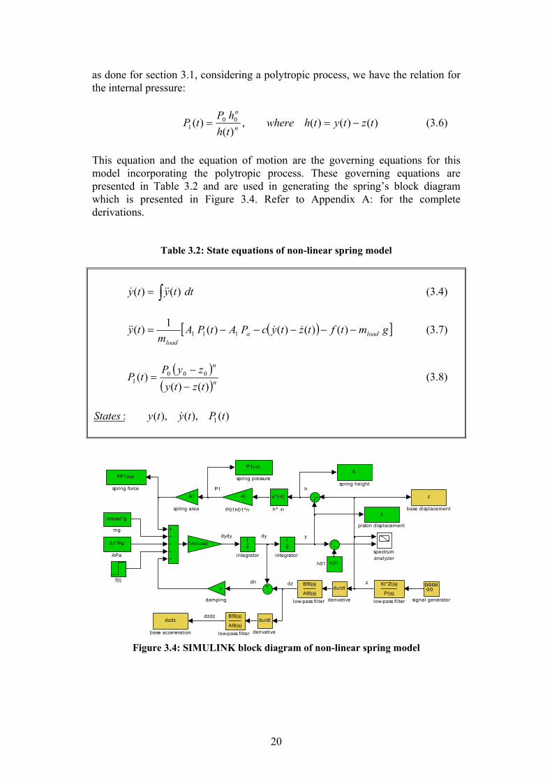
as done for section 3.1, considering a polytropic process, we have the relation for the internal pressure:

)()()(,)(

)( 001 tztythwhere

thhP

tP n

n

−== (3.6)

This equation and the equation of motion are the governing equations for this model incorporating the polytropic process. These governing equations are presented in Table 3.2 and are used in generating the spring’s block diagram which is presented in Figure 3.4. Refer to Appendix A: for the complete derivations.

Table 3.2: State equations of non-linear spring model

dttyty ∫= )()( &&& (3.4)

( )[ ]gmtftztycPAtPAm

ty loadaload

−−−−−= )()()()(1)( 111 &&&& (3.7)

( )

( )n

n

tztyzyP

tP)()(

)( 0001

−

−= (3.8)

)(),(),(: 1 tPtytyStates &

dh

P1

dz z

y

h

dydydy

dzdz

P1out

spring pressureh

spring heightFP1out

spring forceA1

spring area

spectrumanalyzer

signal generator

y

piston displacementmload*g

mg

Bf8(s)

Af8(s)low-pass fil ter

Bf8(s)

Af8(s)low-pass fil ter

1s

integrator

1s

integrator

u^(-n)

h^ -n

h01h01

f(t)

du/dt

derivative

du/dt

derivative

c

damping

z

base displacement

dzdz

base acceleration

-K-

P01h01^n

A1*Pa

APa

Kl*Zl(s)

Pl(s) low-pass fi l ter

1/mload

Figure 3.4: SIMULINK block diagram of non-linear spring model

21

3.3. Complex non-linear spring model To enable more accurate modelling of the spring’s behaviour, boundary work was incorporated into this model. As in the preceding section, the model determines the spring force by means of the spring’s internal pressure. In this model, the pressure is determined by a differential form of the ideal gas equation. To develop this model, the following assumptions were made:

• the air inside the spring is treated as an ideal gas, • the area over which the spring pressure acts is constant, • heat transfer takes place between the spring and its surroundings, and • the unknown damping in the spring can be represented by viscous

damping. The assumption of ideal gas behaviour is relevant since the relative pressure and temperature are in the regions where ideal gas behaviour can be assumed, namely Pr << 1 and Tr > 2 (Çengel and Boles, 2002). Thus, to obtain the change in pressure, we take the ideal gas equation as an equation of state and differentiate it with respect to time. After substitutions and simplifications detailed in Appendix A, the equation of state is obtained

( ))(2)()()(

1)( 111

11 tTTh

CR

rth

thtP

CRtP aQ

vv

−+⎟⎟⎠

⎞⎜⎜⎝

⎛⎟⎟⎠

⎞⎜⎜⎝

⎛+−= && (3.9)

The equation of motion in essence remains the same as defined in section 3.2. Thus the three equations of state defining the model are presented in Table 3.3 below. The block diagram for this model is presented in Figure 3.5.

Table 3.3: State equations of complex non-linear spring model

∫= dttyty )()( &&& (3.4)

( )[ ]gmtftztycPAtPAm

ty loadaload

−−−−−= )()()()(1)( 111 &&&& (3.7)

( ) ( ))(2)()()()(

)(1)( 11

1

11 tTTh

CR

rtzty

tztytP

CRtP aQ

vv

−+−⎟⎟⎠

⎞⎜⎜⎝

⎛−⎟⎟

⎠

⎞⎜⎜⎝

⎛+−= &&& (3.9)

)(),(),(: 1 tPtytyStates &

22

z

y

dzdh

dP1P1A*P1

h

dydydy

dzdz

P1out

spring pressure

FP1out

spring force

A1

spring area

A1

spring area

spectrumanalyzer

signal generator1

h

piston height

y

piston displacement

mload*g

mg

Kl*Zl(s)

Pl(s)low-pass fi lter1

Bf8(s)

Af8(s)low-pass fi lter

Bf8(s)

Af8(s)low-pass fi lter

1s

integrator

1s

integrator

1s

integrator

-K-

hQ1(2R/rCv)

h01h01

f(t)

du/dt

derivative2

du/dt

derivative

c

damping

z

base displacement

dzdz

base acceleration

P1(dh/h)

P1(A1)

A1*Pa

APa

-K-

1/Rm1

-K-

-(1+R/Cv)

T01

1/mload

Figure 3.5: SIMULINK block diagram for complex non-linear spring model

including boundary work

These three models were used in simulations to predict the air-spring behaviour. The equation of motion incorporating base excitations provides a means of numerically simulating vibration inputs typically experienced by seats. The models thus allow simulation of typical conditions that the seat will be exposed to. The successive models are used as a comparative method, with the linear spring model providing the initial model for predicting the system response. The two more complex formulations are firstly gauged against this model to see if their behaviour is within reasonable bounds. Subsequently, the accuracies of the three models are pitted against the actual air-spring response obtained through testing. These results are presented and discussed in Chapter 5. Based on the thermodynamic air-spring model, a model incorporating an auxiliary volume was developed. This includes the full air-spring model with an additional volume connected by a fluidic resistance. The following section deals with the derivation of the governing equations of this model.

3.4. Air-spring model with auxiliary volume After completing the spring models, the next phase of modelling included the auxiliary volume being added to the air-spring model. Since there is mass transfer between the two chambers, continuity and mass equations were added to the existing state equation and the equation of motion.

23

The same assumptions made for the previous model hold here with one addition: • the flow in the restriction can be modelled by internal flow equations.

The equation of motion remains as determined for the spring model in section 3.3, since the parameters defining the motion of the piston are unchanged with the addition of the auxiliary volume as illustrated in Figure 3.6 below.

Figure 3.6: Model of spring with auxiliary volume and free body diagram

The differential form of the ideal gas equation however gains two more terms, one for continuity and the other for conservation of energy. As in section 3.3, the ideal gas equation for the spring volume is differentiated with respect to time. Furthermore, due to mass flow between the air-spring and auxiliary volume, the continuity equation is incorporated into the model. The sign convention adopted for the air-spring is a positive mass flow out of the spring into the auxiliary volume. The continuity equations can thus be defined as

mdt

dmandmdt

dm&& =−= 21 , (3.10), (3.11)

To define the mass flow through the air connection, firstly calculations were done to determine the Reynolds number for flow passing through the restriction. The flow was determined as predominantly turbulent. Based on this, an equation was set up that defined the pressure loss occurring due to the flow restriction. It comprised of three components: friction, contraction and expansion losses. The minor losses were determined by the contraction and expansion coefficients for a square edged entrance and a sudden enlargement.

mload

h(t)

Pa

P1(t), V1(t), m1(t) A1

h(t) mload g

fP1(t)

fPa f(t)

z(t)

y(t)

z(t)

y(t)

P2(t), V2(t), m2(t)

)(tm&

fc(t)

24

The major pressure loss was due to friction and was determined by the Darcy-Weisbach equation, valid for both laminar and turbulent flows (Potter & Wiggert, 2002).

gtV

dlfthL 2

)()(2

= (3.12)

The friction factor, f, was determined for Re > 4000 and completely turbulent flow with

2

7.3ln86.0

−

⎟⎠⎞

⎜⎝⎛−=

def (3.13)

Using the energy equation for pipe flow (Potter & Wiggert, 2002) and equating it with the head loss equation, neglecting the height difference of the capillary entrance and exits since this and the specific weight of air are very small, then re-arranging equation 3.12 we obtain an expression of the velocity. This equation is substituted into the mass flow rate equation and simplified. Considering the cross sectional area of the flow restriction as round, we obtain

( )

( ))()()()()(2

)( 2121

24 tPtPsign

KKKdlf

tPtPtdtm

xEC

avg−

+++

−=

ρπ

& (3.14)

( )( ))()(

)()(

21

21

tTtTRtPtPwhere avg +

+=ρ (3.15)

Furthermore, the energy balance is set up for the spring volume. Section 3.3 dealt with the energy balance for a closed system. Note that there is energy transfer between the spring and auxiliary volume which needs to be accounted for in the energy balance. After substitution and simplification, we obtain a rate equation for the change in temperature:

v

ssQ

v

p

v CtmtTTtAh

CtmtTCtm

CtmthtPAtT

)())(()(

)()()(

)()()()(

1

1111

1

1

1

1111

−+−−=

&&& (3.16)

This temperature rate equation and the mass flow rate are substituted into the change in pressure equation and simplified making use of the ideal gas equation as follows:

25

( ))(2)()()(1

)()()(1)( 11

11

1

1

111 tTTh

CR

rtmtPtm

CC

thtPth

CRtP aQ

vv

p

v

−+⎟⎟⎠

⎞⎜⎜⎝

⎛+−⎟⎟

⎠

⎞⎜⎜⎝

⎛+−= &&&

(3.17) Following a similar procedure for the auxiliary volume, but neglecting heat transfer, the pressure differential becomes

)()()(1)(

2

22 tm

tPtmCC

tPv

p &&⎟⎟⎠

⎞⎜⎜⎝

⎛+= (3.18)

The state equations for this spring and auxiliary volume model derived in Appendix A: are summarised in Table 3.4 below.

Table 3.4: State equations of complex spring model with auxiliary volume

∫= dttyty )()( &&& (3.4)

( )[ ]gmtftztycPAtPAm

ty loadaload

−−−−−= )()()()(1)( 111 &&&& (3.7)

( )

( ))()()()()(2

)( 2121

24 tPtPsign

KKKdlf

tPtPtdtm

xEC

avg−

+++

−=

ρπ

& (3.14)

( )( ))()(

)()()(

21

21

tTtTRtPtP

tavg ++

=ρ (3.15)

)()(),()( 21 tmtmandtmtm &&&& =−= (3.19), (3.20)

( ))(2)()(

)(1)()(

)(1)( 1111

1

1

111 tTTh

CR

rtmtP

tmCvC

thtP

thCRtP aQ

v

p

v

−+⎟⎟⎠

⎞⎜⎜⎝

⎛+−⎟⎟

⎠

⎞⎜⎜⎝

⎛+−= &&&

(3.17)

)()(

)(1)(2

22 tm

tPtm

CC

tPv

p &&⎟⎟⎠

⎞⎜⎜⎝

⎛+= (3.18)

)(),(),(),(),(: 21 tPtPtmtytyStates &

26

These equations are used in setting up the block diagram for the Simulink model depicted in Figure 3.7. This model, representing the complete air-spring and auxiliary volume device, is used in numerical simulations. The simulation results are compared to the test results obtained for the experimental apparatus in Chapter 5.

Figure 3.7: SIMULINK block diagram of spring and auxiliary volume model

z

y

dzdh

dP1

P1

A*P

1

h

dydy

dy

dmm

1

m2

dP2

P2 m

T1

(T1

+ T

2)

(P1

+ P

2)

delta

P(rh

o)(R

)

(P1

- P2)

dzdz

T2

m

trans

ferre

d ai

r mas

s

u^(1

/2)

squa

re ro

ot

u^(1

/2)

squa

re ro

ot

P1

sprin

g pr

essu

re

h

sprin

g he

ight

FP

sprin

g fo

rce

A1

sprin

g ar

ea

A1

sprin

g ar

ea

m1

sprin

g ai

r mas

s

spec

trum

anal

yzer

sign

al g

ener

ator

dydy

pist

on d

ispl

acem

ent1

y

pist

on d

ispl

acem

ent

mlo

ad*g

mg

dm

mas

s flo

w ra

te

mas

s flo

w ra

te

Bf8

(s)

Af8

(s)

low

-pas

s fil

ter

Bf8

(s)

Af8

(s)

low

-pas

s fil

ter

Kl*

Zl(s

)

Pl(s

)lo

w-p

ass

filte

r

hL

loss

fact

or

1 s

inte

grat

or

1 s

inte

grat

or

1 s

inte

grat

or

-K-

hQ1(

2R/r1

Cv)

h01

h01

f(t)

du/d

t

deriv

ativ

e

du/d

t

deriv

ativ

e

c

dam

ping

Aca

p

capi

llary

are

a

z

base

dis

plac

emen

t

dzdz

base

acc

eler

atio

n

P

aux

vol p

ress

ure

m2

aux

vol a

ir m

assV

2

Sig

n

P2(

dm/m

2)

P2(

V2/

m2)

P1(

dm/m

1)

P1(

dh/h

)

P1(

A1/

m1)

1 s

Inte

grat

or

1 s

Inte

grat

or

Div

ide6

|u|

Abs

A1*

Pa

AP

a

-K-

-(1+R

/Cv)

-K-

-(1+C

p/C

v)

-K-

(1+C

p/C

v)

T01

1/R

1/m

load

m01

m02

2/R

1/R

27

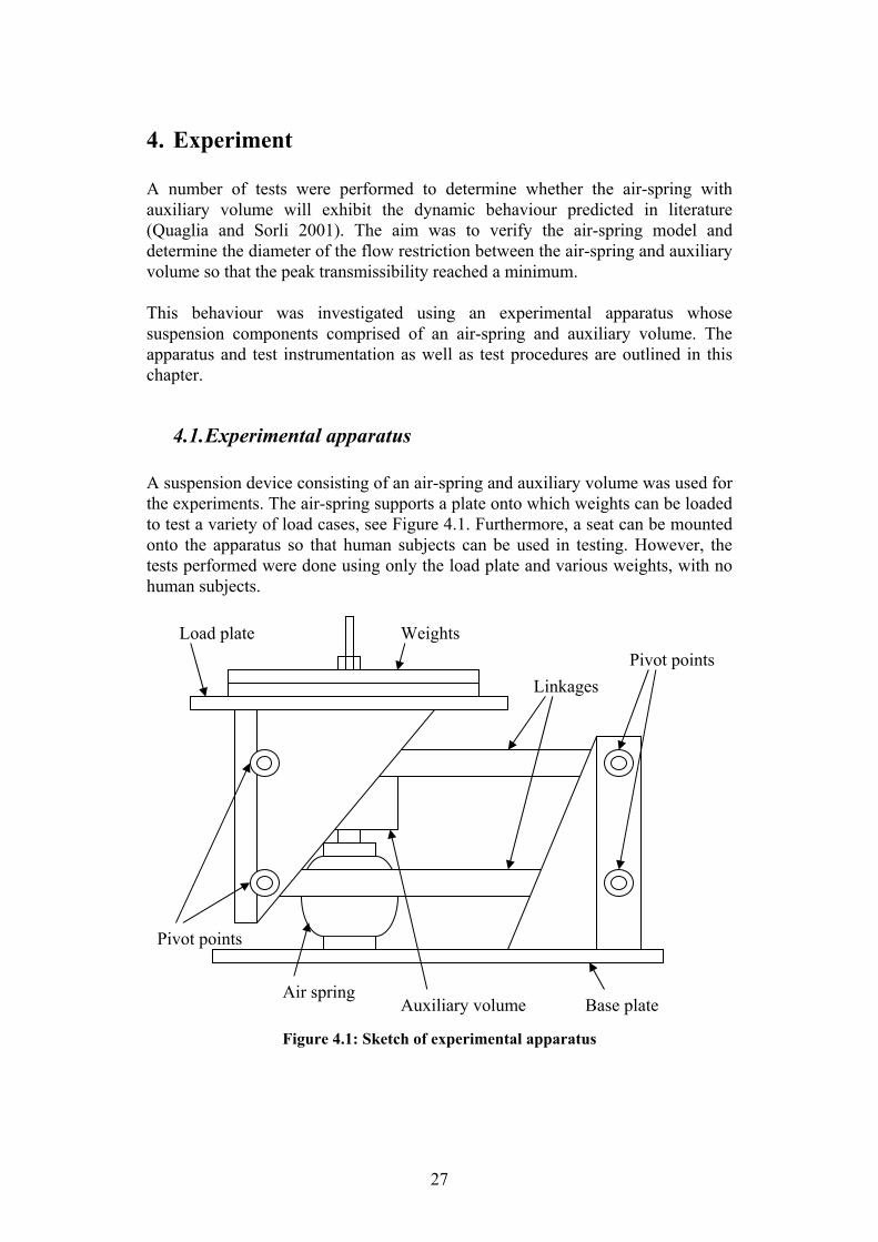
4. Experiment A number of tests were performed to determine whether the air-spring with auxiliary volume will exhibit the dynamic behaviour predicted in literature (Quaglia and Sorli 2001). The aim was to verify the air-spring model and determine the diameter of the flow restriction between the air-spring and auxiliary volume so that the peak transmissibility reached a minimum. This behaviour was investigated using an experimental apparatus whose suspension components comprised of an air-spring and auxiliary volume. The apparatus and test instrumentation as well as test procedures are outlined in this chapter.

4.1. Experimental apparatus A suspension device consisting of an air-spring and auxiliary volume was used for the experiments. The air-spring supports a plate onto which weights can be loaded to test a variety of load cases, see Figure 4.1. Furthermore, a seat can be mounted onto the apparatus so that human subjects can be used in testing. However, the tests performed were done using only the load plate and various weights, with no human subjects.

Figure 4.1: Sketch of experimental apparatus

Load plate

Linkages Pivot points

Air spring Auxiliary volume Base plate

Weights

Pivot points

28

To determine spring characteristics, the device was designed to approximate linear motion for the load and the air-spring. This was done using a Watt’s linkage. The links of equal lengths are placed in a horizontal position with the air-spring at its equilibrium height. The sketch in Figure 4.1 shows the pivot points of the upper linkage are located vertically above the corresponding pivots of the lower linkage. This, and the fact that the linkages were relatively long, ensured approximate linear motion for the load plate in the vertical direction. Compressed air was supplied to the spring to allow adjustment of the spring internal pressure and to raise or lower the load plate to equilibrium height, depending on the load placed onto it. To test the dynamic behaviour of the air-spring and auxiliary volume combination, connectors with various hole diameters were manufactured as depicted in Figure 4.2. These flow restrictions could be interchanged to test the air-spring and auxiliary volume behaviour for the various load cases. To test the air-spring by itself, the air path between the two was simply blanked off.

Figure 4.2: Air supply to spring and flow connector between air-spring and

auxiliary volume (top), and configuration of connector (bottom)

Ø 0,0 mm – Ø 6,5 mm

29 mm

M10x1 M10x1

22 mm

Connector Compressed air supply

Air-spring

29

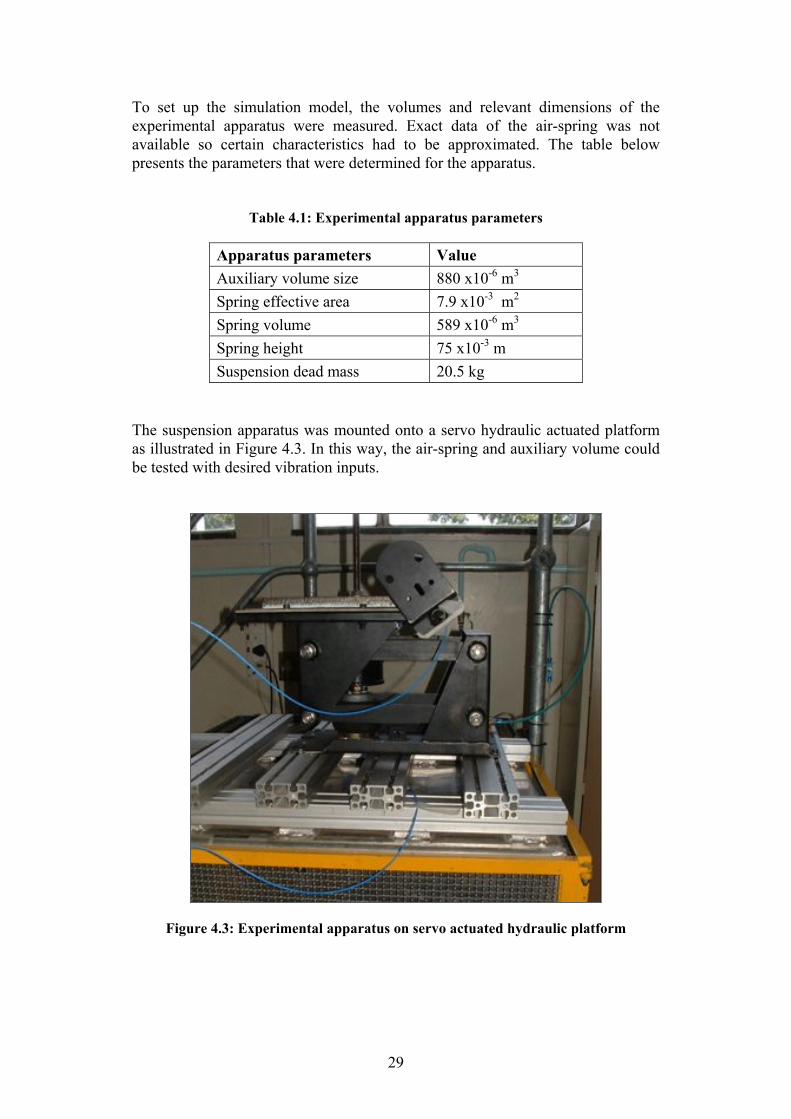
To set up the simulation model, the volumes and relevant dimensions of the experimental apparatus were measured. Exact data of the air-spring was not available so certain characteristics had to be approximated. The table below presents the parameters that were determined for the apparatus.

Table 4.1: Experimental apparatus parameters

Apparatus parameters Value Auxiliary volume size 880 x10-6 m3

Spring effective area 7.9 x10-3 m2 Spring volume 589 x10-6 m3 Spring height 75 x10-3 m Suspension dead mass 20.5 kg

The suspension apparatus was mounted onto a servo hydraulic actuated platform as illustrated in Figure 4.3. In this way, the air-spring and auxiliary volume could be tested with desired vibration inputs.

Figure 4.3: Experimental apparatus on servo actuated hydraulic platform

30

4.2. Test equipment and procedures The servo hydraulic actuated platform of the dynamic seat test facility was designed to simulate conditions experienced in typical vehicles or vessels. Thus any desired vibration input could be simulated to test the device. To determine the spring characteristics, the suspension device comprising of the air-spring and auxiliary volume was mounted on the dynamic seat test facility. To measure the transmissibility of the suspension device, two accelerometers were mounted on the device. One was mounted on the base plate to measure the base or input acceleration, and the second was mounted on the load plate to measure the output acceleration. The signals from the accelerometers were routed to the data acquisition system that provided an interface between the computer and test equipment, shown in Figure 4.4. The software used to acquire and analyse the signals was MATLAB/Siglab. A signal for testing the device was sent from the MATLAB/Siglab workspace via the Siglab box to the controller that regulates the servo hydraulic actuated platform. Figure 4.4 below shows the equipment used in the data acquisition and control of the platform.

Figure 4.4: Data processing and control equipment

Computer running MATLAB/Siglab

Accelerometer power supply

Siglab box

Servo hydraulic actuator

Servo hydraulic controller

Platform

31

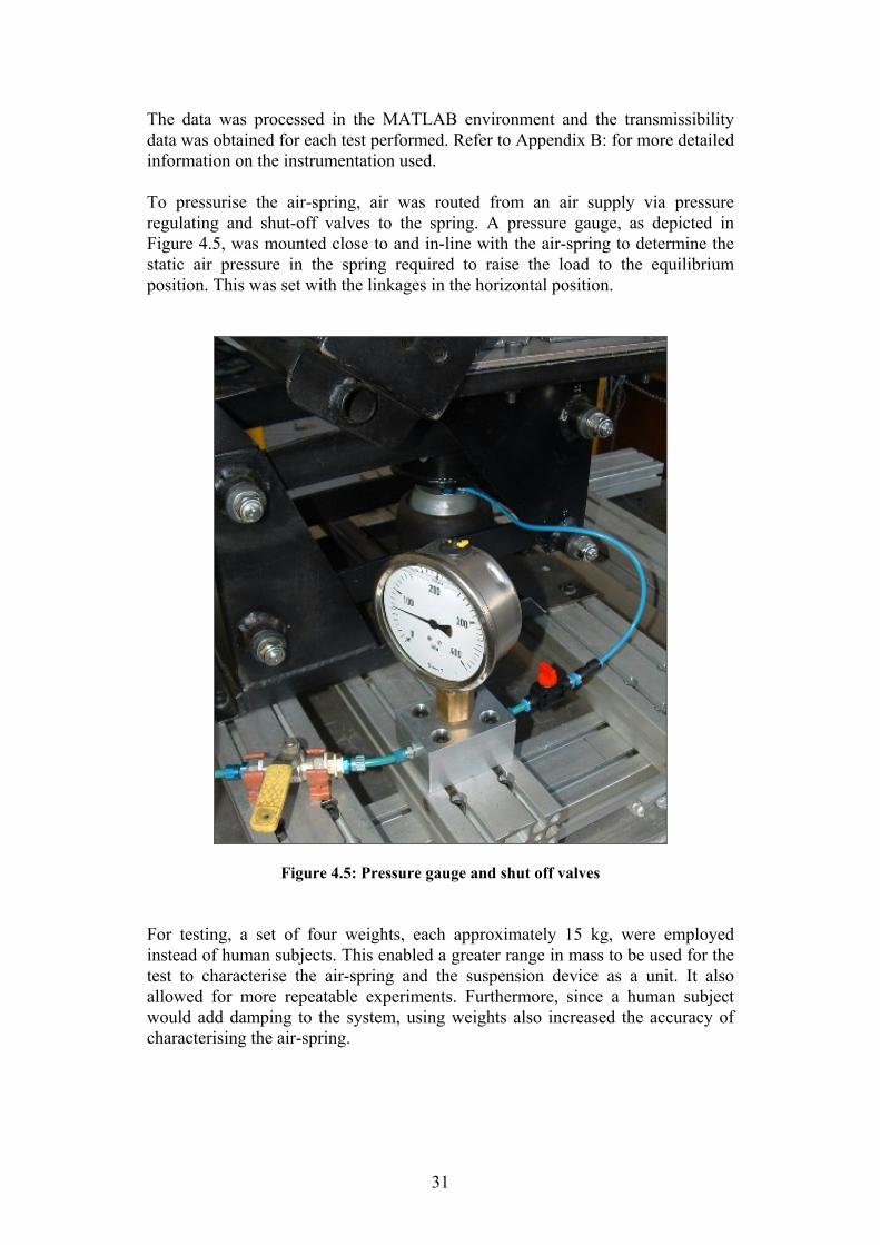
The data was processed in the MATLAB environment and the transmissibility data was obtained for each test performed. Refer to Appendix B: for more detailed information on the instrumentation used. To pressurise the air-spring, air was routed from an air supply via pressure regulating and shut-off valves to the spring. A pressure gauge, as depicted in Figure 4.5, was mounted close to and in-line with the air-spring to determine the static air pressure in the spring required to raise the load to the equilibrium position. This was set with the linkages in the horizontal position.

Figure 4.5: Pressure gauge and shut off valves For testing, a set of four weights, each approximately 15 kg, were employed instead of human subjects. This enabled a greater range in mass to be used for the test to characterise the air-spring and the suspension device as a unit. It also allowed for more repeatable experiments. Furthermore, since a human subject would add damping to the system, using weights also increased the accuracy of characterising the air-spring.

32

For each of the four load cases, three test runs were performed. The amplitude of the forcing signal was increased to give three different sets of results, each with increased r.m.s. acceleration values. A table listing the settings for each experiment is presented below.

Table 4.2: Settings used for simulations and test runs

Load case * 1 2 3 4 Mass [kg] 15.42 30.83 46.26 61.68 * these values include the additional 20.5 kg of the suspension components

Voltage [V] 2 V = ± 1 m/s2 r.m.s.

4 V = ± 2 m/s2 r.m.s.

6 V = ± 3 m/s2 r.m.s.

Before the first test run was started, the system was cycled with a 10 mm sinusoidal input at 10 Hz for 5-10 minutes to allow the oil and components to reach their operating temperature. The testing procedure was performed as follows:

• load and fix mass onto load plate • adjust spring internal pressure to level linkages in the horizontal

equilibrium position • record pressure reading • switch on hydraulic pumps and cycle system 1-2 minutes at test signal

before sampling data • sample data • stop system and switch off all hydraulic pumps • set linkages to level position • check pressure reading to determine if any air leaked out • perform next run at higher voltage setting.

The second round of tests involved the combination of the spring and auxiliary volume. A number of connectors were employed to create a path for air flow between the air-spring and auxiliary volume. The diameters of these connections were varied to change the flow rate between the air chambers. Furthermore the number of load cases was reduced to two to decrease the amount of test runs required. The tests performed were done with load cases 1 and 3. As previously discussed, it is evident that the parameter of primary interest is the diameter of the flow restriction since it determines the system’s natural frequency and transmissibility magnitude. The aim is thus to verify the behaviour as predicted by literature and to determine the optimal diameter for the specified setup. Of further interest is the relationship between hole diameter and mass, more

33

specifically how a change in mass influences the response for an optimal hole diameter that gives a minimum transmissibility for a specified mass. This behaviour of the apparatus and that of the simulation models is investigated in the following chapter where the test and simulation results are discussed. A typical result is presented in Figure 4.6 where the transmissibility curve of the air-spring tested for load case 3 at 2 m/s2 r.m.s. is depicted.

0.5 1 1.5 2 2.5 3 3.5 4 4.5 5 5.5 60

0.5

1

1.5

2

2.5

3

3.5

4

Frequency [Hz]

Tran

smis

sibi

lity

Transfer Function - ExperimentAir-Spring Load Case 3, 2 m/s2 r.m.s.

Figure 4.6: Transmissibility curve for air-spring experiment at load case three

34

5. Results – simulation and testing For the simulations, the same random input signal was used as for the experiments - its acceleration power spectral density filtered above 15 Hz. This signal was chosen to excite all the relevant frequencies in the system to give an accurate depiction of typical vibration inputs such a device would be exposed to. By exciting the system with a signal containing random frequencies, the transmissibility curves could be obtained. The first comparison drawn is that between the various spring models and experimental apparatus. Thereafter the auxiliary volume model is investigated and compared to the experimental results. The chapter is concluded with a discussion of the results.

5.1. Air-spring simulation and experiment results The air spring simulation models parameters were chosen based on the dimensions of the specific air-spring used for testing. The simulations involved four load cases for each model as shown in Table 4.2. The linear model was created as a simple comparison to evaluate results obtained for the more complex models. The tests performed on the air-spring would verify the simulation results and determine their overall accuracy to simulate the physical device. This would also determine if the models could be used to incorporate the auxiliary volume. Thus, a comparison of the experimental data and simulation data follows with a discussion of the results. Since the air spring is a complex device, many parameters are difficult to define. A case in point is the rubber chord material where for instance the spring walls exhibit certain stiffness and damping. Furthermore the effective spring area varies with height as the diaphragm folds during the stroke. These factors were excluded from this model to reduce its complexity. As the model does not account for all forms of damping, a viscous damping term was introduced. This allowed adjustment to the system’s damping so that the amplitude of the complex simulation model could be matched to that of the experimental apparatus. For the model comparison, the simulations were run for each spring model at a specific load setting. The results of load case 3 are presented in Figure 5.1. The linear and non-linear models show a lower amplitude than the complex non-linear model. The definite increase of peak transmissibility can be attributed to the more non-linear response from the air spring as rapid compression leads to an

35

exponential pressure increase inside the spring. This in turn increases the spring ‘stiffness’ and thus directly the spring force. Considering the linear and non-linear models whose state equations were presented in section 3.1 and 3.2 respectively, the spring stiffness for the linear model was determined from the relation of an adiabatic polytropic process, otherwise known as an isentropic process. The result is a spring stiffness matched to that of the non-linear model, whose stiffness or spring force is derived from the spring internal pressure that is calculated directly from the polytropic relation. This is of course applicable for motions about the equilibrium position as encountered here.

0.5 1 1.5 2 2.5 3 3.5 4 4.5 5 5.5 60

0.5

1

1.5

2

2.5

3

3.5

4

4.5

5

5.5

Transfer function - air-springSimulation load case 3, 3 m/s2 r.m.s.

Frequency [Hz]

Tran

smis

sibi

lity

Linear Non-linear Complex

Figure 5.1: Comparison of transmissibility for air spring models at load case three

Despite the complex model’s higher peak transmissibility, the natural frequencies correlate well. It would therefore seem reasonable to assume that both methods, the polytropic relation and the differential form of the ideal gas equation, provide comparable results. Having obtained satisfactory results regarding the natural frequency and approximate amplitudes of the model, the test results for the air-spring were considered next.

36

The experimental apparatus was run with four load settings, and the result of load case 3 is presented in Figure 5.2. The experimental result and that of the complex air-spring model are very similar. The natural frequency of the simulations and experiment match up quite accurately. Variation between the peak transmissibility of the complex model and the experimental apparatus was removed by adjusting the damping factor. After this parameter was determined, it remained fixed at this value for any following simulations.

0.5 1 1.5 2 2.5 3 3.5 4 4.5 5 5.5 60

0.5

1

1.5

2

2.5

3

3.5

4

4.5

5

5.5

Transfer function - air-springSimulation and experiment - load case 3 @ 3 m/s2 r.m.s.

Frequency [Hz]

Tran

smis

sibi

lity

Linear Non-linear Complex Experiment

Figure 5.2: Comparison between transmissibility for air spring models and

experimental apparatus at load case three For the intermediate amplitude setting of 3 m/s2 r.m.s. selected for the tests, the natural frequencies and transmissibility amplitudes matched those obtained for the simulation models. This leads to the conclusion that, for general simulation purposes, the air-spring model is a good approximation to the experimental apparatus. Despite the simplifications made in developing this model, the results show that the air-spring can be modelled with reasonable accuracy, and thus the somewhat more complex model of the auxiliary volume is presented in the following section.

37

5.2. Auxiliary volume simulation and experiment results The preceding section dealt with the behaviour of only the air-spring. Attention is now turned to the air spring and auxiliary volume combination. As outlined in Chapters 1 and 2, literature predicts a certain type of behaviour for this configuration. The flow restriction between the air spring and auxiliary volume allows air to pass between the two volumes. This will result in a system response where the minimum transmissibility is attained at a natural frequency between those of solely the air spring and the air spring and auxiliary volume combination. This behaviour is investigated here. The model being scrutinised in this section is based on the complex air-spring model incorporating an auxiliary volume. As in the preceding section, a random input signal was used to excite the base of the suspension device. For the simulations and the experiment, load cases one and three were investigated. The aim was to determine if the system response for a particular flow restriction diameter was load dependent. Thus for each of the load cases, the diameter was varied to obtain the frequency response and thus the transmissibility curves of the suspension configuration. The simulation results for load case three are presented in Figure 5.3.

0.5 1 1.5 2 2.5 3 3.5 4 4.5 5 5.5 60

0.5

1

1.5

2

2.5

3

3.5

4

Transfer Function - air-spring and aux. volumeSimulation load case 3 @ 3 m/s2 r.m.s.

Frequency [Hz]

Tran

smis

sibi

lity

∅ 1.0 mm ∅ 1.5 mm ∅ 2.0 mm ∅ 2.5 mm ∅ 3.5 mm

Figure 5.3: Transmissibility curves of spring auxiliary volume model

with load case 3

38

It can clearly be seen how the transmissibility magnitude of the air-spring and auxiliary volume combination decreases with the addition of an air-flow path between these two air volumes. Initially, for small diameters of the flow restriction, the system distinctly shows additional damping. Increasing the diameter brings about a twofold change in the system: increased damping, and a shift in the system’s natural frequency. The initial transmissibility peak for the small hole diameter occurs at the natural frequency of the spring. The shift in the natural frequency occurs when the diameter is increased further, thus allowing mass transfer between the two volumes. This interaction between the two air spaces becomes more noticeable as the diameter is increased further, with the transmissibility magnitude decreasing, effectively increasing the system’s damping and decreasing the natural frequency. Having derived the equation for equivalent spring stiffness shown in equation 3.2, it is clear that an increase in volume by increasing the spring height reduces the stiffness of the system. Thus the increase in the flow restriction diameter and hence mass flow, gives the system a characteristic reduction in the natural frequency; the system now behaves like it has a larger volume and therefore lower stiffness.

0

01

hPnA

kequ−

= (3.2)

The main advantage is the pronounced reduction in the magnitude of transmissibility found between the two extreme cases of just the air-spring, and when the auxiliary volume is added to this. Inherent damping is introduced into the system, reducing the peak transmissibility by more than 60 % when compared to the results obtained for the air-spring as presented in section 5.1. The results obtained when simulating the system response using load case one, show a similar trend of decreasing transmissibility magnitude and shift in natural frequency as obtained with load case three. Refer to Appendix C. It can however be seen that a slightly larger diameter brings about the minimum transmissibility. Turning attention from the numerical simulation models to the results obtained from the experiment, these seem to exhibit similar behaviour to that predicted by the models. For the same specified diameters, the model predicts the same trend in transmissibility and shift in natural frequency during experiments as illustrated in Figure 5.4. The peak transmissibility at the air-spring’s natural frequency reduces and shifts to a lower natural frequency as the diameter is increased from 1,0 mm to its minimum at 2,5 mm. Thereafter it increases further as the diameter increases to the maximum of 6,5 mm. The trend of the shifting natural frequency and reduction in peak transmissibility in literature is thus verified by simulation and

39

experiment. It needs to be noted that the model was not able to run simulations with flow restriction diameters of 6,5 mm or larger, as seen in Figure 5.3. The 6,5 mm results are thus absent from the simulation data.

0.5 1 1.5 2 2.5 3 3.5 4 4.5 5 5.5 60

0.5

1

1.5

2

2.5

3

3.5

4

Transfer Function - air-spring and aux. volumeSimulation and experiment load case 3, 3 m/s2 r.m.s.

Frequency [Hz]

Tran

smis

sibi

lity

∅ 1.0 mm ∅ 1.5 mm ∅ 2.0 mm ∅ 2.5 mm ∅ 3.5 mm ∅ 6.5 mm

Figure 5.4: Transmissibility curves of experiment with air-spring

The model results thus predict the trend as seen in the experimental apparatus; the simulation model and experimental results match up for the smallest diameter and as the diameter is increased, the model results follow the same trend. The most noticeable difference however, when overlaying the results for the simulation and experiment, is the minimum transmissibility and the lower natural frequency of the combined air-spring and auxiliary volume response, shown in Figure 5.5. The auxiliary volume was identified to have a pronounced influence on transmissibility magnitude and the lower natural frequency. Figure 5.6 shows the system response for the original auxiliary volume size reduced by a third: V/3. Now the transmissibility curves of the experiment and simulation match, bar the higher transmissibility. This and the fact that an additional pressure loss coefficient, Kx, had to be introduced to obtain this result, implies the flow restriction in the experimental device provides more damping than initially modelled. In the light of this, it can be argued that the auxiliary volume model behaves as if the auxiliary volume is larger than it actually is. The simulation results thus predict a lower natural frequency and magnitude of transmissibility.

40

0.5 1 1.5 2 2.5 3 3.5 4 4.5 5 5.5 60

0.5

1

1.5

2

2.5

3

3.5

4

4.5

Transfer Function - air-spring and aux. volumeSimulation and experiment load case 3, 3 m/s2 r.m.s.

Frequency [Hz]

Tran

smis

sibi

lity

∅ 1.0 mm (sim) ∅ 2.5 mm (sim) ∅ 3.5 mm (sim) ∅ 1.0 mm (exp) ∅ 2.5 mm (exp) ∅ 3.5 mm (exp)

Figure 5.5: Transmissibility curves of air-spring and auxiliary volume

0.5 1 1.5 2 2.5 3 3.5 4 4.5 5 5.5 60

0.5

1

1.5

2

2.5

3

3.5

4

4.5

Transfer Function - air-spring and aux. volume V/3Simulation load case 3, 3 m/s2 r.m.s.

Frequency [Hz]

Tran

smis

sibi

lity

∅ 1.0 mm ∅ 1.5 mm ∅ 2.0 mm ∅ 2.5 mm ∅ 3.5 mm

Figure 5.6: Transmissibility curves of air-spring and auxiliary volume

with V/3 and increased Kx

41

5.3. Discussion of simulation and experiment results The air-spring model predicts the spring natural frequency accurately, although the peak transmissibility between the simulation and experiment does vary somewhat for different load cases when adopting a constant damping ratio. Simulation peak transmissibilities however remain reasonably constant between the load cases. Overall, the air-spring simulation models predict the experimental behaviour well. The addition of the auxiliary volume introduces a trend in dynamic behaviour with variation of flow restriction diameters by decreasing transmissibility and natural frequency with an increase in diameter up to the point of lowest transmissibility. The fact that the minimum transmissibility and lower natural frequency for the combined air-spring and auxiliary volume is lower for the simulation model than the experiments dictate, can assumed to be attributed to more complex dynamic behaviour of the air passing between the two chambers. Looking at the simulation model or experimental apparatus, the change in the natural frequency can be attributed to the increasing influence the auxiliary volume has on the system as the increase in diameter facilitates higher mass flow rates between the two chambers. As the mass flow increases, it is no longer just the volume of the spring that determines the spring stiffness. Having derived the equation for equivalent spring stiffness, equation 3.2, it is clear that an increase in volume by increasing the spring height reduces the stiffness of the system. Thus the increase in the flow restriction diameter and hence mass flow, gives the system a characteristic reduction in the natural frequency; the system now behaves like it has a larger volume and therefore lower stiffness. Essentially, for large flow restriction diameters, the volume of the air-spring is increased by an amount equal to that of the auxiliary volume. The overall effect is a softer spring as during spring compression the air can ‘escape’ into the larger available cavity. The models have shown a fair deal of forecasting capability for the actual device. Refinement regarding auxiliary volume modelling, more particularly flow modelling, could aid in improving the accuracy of simulation results. Such detail analysis lies outside the scope of this project.

42

6. Procedure to design novel air-spring suspension Having developed an air-spring and auxiliary volume model, this can be used to design a prototype air-spring device for a suspension seat. This chapter presents both the design parameters that can be adjusted to modify the system response, and the design procedure to generate a first round prototype. This is done considering the ISO 7096 standard which stipulates typical vibration inputs for earth moving machinery in the light of evaluating operator seat vibration. Subsequent to that, simulations are run to evaluate the air-spring device performance. A means to evaluate the air-spring performance is the SEAT value and this parameter is employed to determine how suitable the design is for use in particular vehicles. The aim is thus to design the seat suspension to obtain acceptable levels of vibrations as determined by the SEAT value.

6.1. Design parameters and criteria To design an air suspension that gives the desired response of good vibration isolation, specific design parameters or variables need to be identified. These enable the designer to systematically adjust the parameters to obtain the design objective of developing an air-spring and auxiliary volume suspension providing good vibration isolation. Four main factors were identified when the models were developed that affect the air-spring and auxiliary volume combination frequency response. They are the:

• air-spring effective area, • suspended load, • flow restriction diameter, and • auxiliary volume size.

Bearing in mind that only one air-spring was available, making the effective area a constant, and that the load is considered a system input, only the remaining two factors of the flow restriction diameter and auxiliary volume size were considered as design variables. The suspended load had the overall effect of decreasing the natural frequency of the system. Thus the range in operator weight needed to be taken into consideration, and to ascertain whether large variation occurred with regard to the optimum diameter as the load was varied or if this was insignificant.

43

It was ascertained in the preceding sections that the increase in the flow restriction diameter from a very small to larger ones decreased the system natural frequency and also the peak transmissibility. When changing this parameter, it was of interest to find the diameter size providing the lowest transmissibility. In the light of this, the diameter size was considered a significant parameter, essential to obtain a low transmissibility. The remaining factor to be considered is the auxiliary volume size. Literature indicates that the peak occurring at the largest diameter size is considered the peak of the combined volumes of the air-spring and auxiliary volume. It can thus be assumed that the larger the total volume, the lower the first natural frequency of the system. Figure 6.1 illustrates the typical system response for two load cases as the flow restriction diameter is varied. Thus, to lower the natural frequency and peak transmissibility of the system, a larger auxiliary volume with a large flow restriction diameter is required.

0.5 1 1.5 2 2.5 3 3.5 4 4.5 5 5.5 60

0.5

1

1.5

2

2.5

3

3.5

4

4.5

5

Frequency [Hz]

Tran

smis

sibi

lity

Transfer function - air-spring and aux. volumeSimulation load cases 1 and 3, 3 m/s2 r.m.s

∅ 1.0 mm (1) ∅ 2.5 mm (1) ∅ 3.5 mm (1) ∅ 1.0 mm (3) ∅ 2.5 mm (3) ∅ 3.5 mm (3)

Figure 6.1: The effects of changing flow restriction diameter

and load on system response To develop the suspension for a specific application, the appropriate simulation conditions were required. The ISO 7096:2000(E) standard on Earth-moving machinery – Laboratory evaluation of operator seat vibration, provides various

44

spectral classes of vibration inputs. The test used for this design application was the EM1 spectral class representing vibration experienced in articulated or rigid frame dumpers. An input signal was used, the acceleration power spectral density of which had a similar r.m.s. acceleration content as that of the EM1 test. The acceleration power spectral density for the EM1 test is shown in Figure 6.2 below.

0 2 4 6 8 10 120

0.5

1

1.5

2

2.5

Target PSD (G*p(f)) forSpectral class EM1 vibration input

Frequency [Hz]

PS

D [(

m/s

2 )2 /Hz]

Figure 6.2: PSD plot and r.m.s. value for spectral class EM1 – ISO 7096

An acceptable SEAT value is provided for each spectral class presented in ISO 7096. For this spectral class, the standard stipulates a SEAT value of < 1,1, meaning that no more than a 10 % increase in transmission of vibration is to be allowed. This value is calculated from the weighted acceleration power spectral density of the seat and floor as defined in section 1.2 by equation 1.2 below

100)()(

)()(%

2/1

2

2

×⎥⎥⎦

⎤

⎢⎢⎣

⎡=∫∫

dffWfG

dffWfGSEAT

iff

iss (1.2)

where Gss(f) and Gff(f) are the seat and floor acceleration power spectra and Wi(f) is the frequency weighting for the human response to vibration which is of interest (Griffin, 1990).

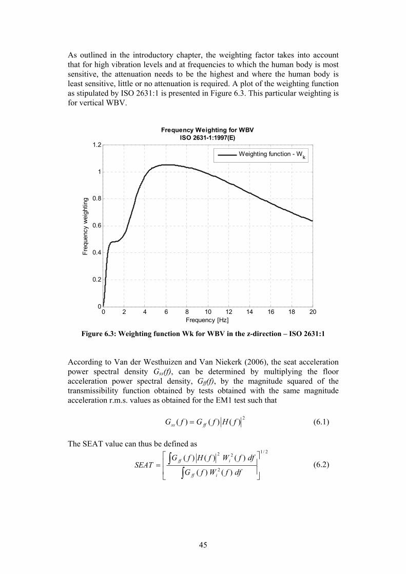
45

As outlined in the introductory chapter, the weighting factor takes into account that for high vibration levels and at frequencies to which the human body is most sensitive, the attenuation needs to be the highest and where the human body is least sensitive, little or no attenuation is required. A plot of the weighting function as stipulated by ISO 2631:1 is presented in Figure 6.3. This particular weighting is for vertical WBV.

0 2 4 6 8 10 12 14 16 18 200

0.2

0.4

0.6

0.8

1

1.2

Frequency Weighting for WBVISO 2631-1:1997(E)

Frequency [Hz]

Freq

uenc

y w

eigh

ting

Weighting function - Wk

Figure 6.3: Weighting function Wk for WBV in the z-direction – ISO 2631:1

According to Van der Westhuizen and Van Niekerk (2006), the seat acceleration power spectral density Gss(f), can be determined by multiplying the floor acceleration power spectral density, Gff(f), by the magnitude squared of the transmissibility function obtained by tests obtained with the same magnitude acceleration r.m.s. values as obtained for the EM1 test such that

2)()()( fHfGfG ffss = (6.1) The SEAT value can thus be defined as

2/1

2

22

)()(

)()()(

⎥⎥

⎦

⎤

⎢⎢

⎣

⎡=

∫∫

dffWfG

dffWfHfGSEAT

iff

iff (6.2)

46

Considering the weighting function, it is clear that the transmissibility peak should be kept at as low a frequency value as possible, since at the lower frequency range, there is a lesser penalty incurred regarding transmitted vibration. From the preceding discussion, it is recognised that the design objective is to lower the natural frequency of the system and decrease the transmissibility magnitude to the extent where the response of the system will result in a SEAT value of less than 1,1.

6.2. Design procedure and simulation Having decided on the design variables and that a SEAT value below 1.1 was required, the design procedure was considered next. This comprised a number of simulations to determine which combination of system parameters would provide the best results. In section 6.1 the auxiliary volume size and flow restriction diameter were recognised as the main design variables. The load was also varied to determine to which extent variation in operator weight would change the response. Two load cases, sample loads one and three, were used again and two additional auxiliary volume sizes were selected besides the original volume, namely instances of twice and thrice the original volume size. The diameters ranged from 1,0 mm to 3,5 mm. This range allowed enough leeway to observe which diameter would be most suitable. Concerning the increase in the auxiliary volume size, attention needs to be turned to the results in section 5.2. It would seem evident that the simulation model behaves as if the auxiliary volume is larger than it actually is – the natural frequency and transmissibility magnitude are less than in reality. To try and match the simulation to the experimental results, the volume could be decreased by a factor of about three. Since this would also require adjustment of the damping constants and flow loss coefficient, too much uncertainty would be introduced making this approach less desirable. This merely substantiates the fact that more accurate modelling of the flow restriction would be necessary. It was therefore opted to rather continue with the model ‘as-is’ for the design procedure. Figure 6.4 again illustrates the typical trend of an increasing flow restriction diameter – decreased transmissibility and natural frequency as was discussed at length in Chapter 5. The result set in Figure 6.4 was obtained with the original volume size.

47

0.5 1 1.5 2 2.5 3 3.5 4 4.5 5 5.5 60

0.5

1

1.5

2

2.5

3

3.5

4

Frequency [Hz]

Tran

smis

sibi

lity

Transfer function - air-spring and aux. volumeSimulation load case 3, 3 m/s2 r.m.s

∅ 1.0 mm ∅ 1.5 mm ∅ 2.0 mm ∅ 2.5 mm ∅ 3.5 mm

Figure 6.4: System response with increasing flow restriction diameter

The results when the volume is tripled can be seen in Figure 6.5.

0.5 1 1.5 2 2.5 3 3.5 4 4.5 5 5.5 60

0.5

1

1.5

2

2.5

3

3.5

4

4.5

Transfer Function - air-spring and aux. volume 3xVSimulation load case 3, 3 m/s2 r.m.s.

Frequency [Hz]

Tran

smis

sibi

lity

∅ 1.0 mm ∅ 1.5 mm ∅ 2.0 mm ∅ 2.5 mm ∅ 3.5 mm ∅ 5.5 mm

Figure 6.5: System response with increased auxiliary volume size

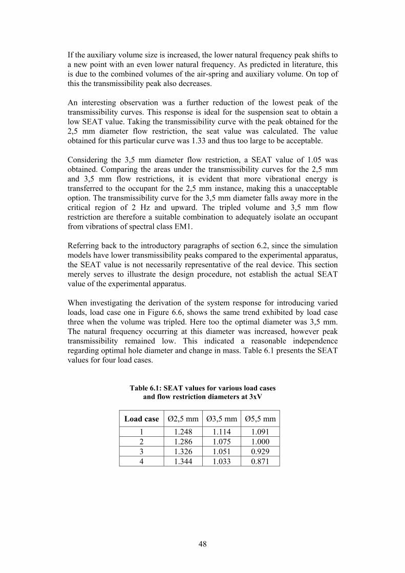
48

If the auxiliary volume size is increased, the lower natural frequency peak shifts to a new point with an even lower natural frequency. As predicted in literature, this is due to the combined volumes of the air-spring and auxiliary volume. On top of this the transmissibility peak also decreases. An interesting observation was a further reduction of the lowest peak of the transmissibility curves. This response is ideal for the suspension seat to obtain a low SEAT value. Taking the transmissibility curve with the peak obtained for the 2,5 mm diameter flow restriction, the seat value was calculated. The value obtained for this particular curve was 1.33 and thus too large to be acceptable. Considering the 3,5 mm diameter flow restriction, a SEAT value of 1.05 was obtained. Comparing the areas under the transmissibility curves for the 2,5 mm and 3,5 mm flow restrictions, it is evident that more vibrational energy is transferred to the occupant for the 2,5 mm instance, making this a unacceptable option. The transmissibility curve for the 3,5 mm diameter falls away more in the critical region of 2 Hz and upward. The tripled volume and 3,5 mm flow restriction are therefore a suitable combination to adequately isolate an occupant from vibrations of spectral class EM1. Referring back to the introductory paragraphs of section 6.2, since the simulation models have lower transmissibility peaks compared to the experimental apparatus, the SEAT value is not necessarily representative of the real device. This section merely serves to illustrate the design procedure, not establish the actual SEAT value of the experimental apparatus. When investigating the derivation of the system response for introducing varied loads, load case one in Figure 6.6, shows the same trend exhibited by load case three when the volume was tripled. Here too the optimal diameter was 3,5 mm. The natural frequency occurring at this diameter was increased, however peak transmissibility remained low. This indicated a reasonable independence regarding optimal hole diameter and change in mass. Table 6.1 presents the SEAT values for four load cases.

Table 6.1: SEAT values for various load cases and flow restriction diameters at 3xV

Load case Ø2,5 mm Ø3,5 mm Ø5,5 mm

1 1.248 1.114 1.091 2 1.286 1.075 1.000 3 1.326 1.051 0.929 4 1.344 1.033 0.871

49

0.5 1 1.5 2 2.5 3 3.5 4 4.5 5 5.5 60

0.5

1

1.5

2

2.5

3

3.5

4

4.5

Transfer Function - air-spring and aux. volume 3xVSimulation load case 1, 3 m/s2 r.m.s.

Frequency [Hz]

Tran

smis

sibi

lity

∅ 1.0 mm ∅ 1.5 mm ∅ 2.0 mm ∅ 2.5 mm ∅ 3.5 mm

Figure 6.6: System response with increasing flow restriction diameter

and increased auxiliary volume size For illustrative purposes, the results in Table 6.1 are presented in Figure 6.7 as a plot of SEAT values against load case and flow restriction diameter.

1

2

3

12

34

0.8

0.9

1

1.1

1.2

1.3

1.4

Diameter

Air-spring and auxiliary volume effectiveness for 3xV

Load case

SE

AT

valu

e

Figure 6.7: Air-spring and auxiliary volume effectiveness

in terms of SEAT value for 3xV

50

This plot clearly shows how, for a specific auxiliary volume size, the increase in mass reduces the SEAT value because of the reduction in the natural frequency of the system. This value can only be decreased to a certain level because the natural frequency has the lower bound of 0 Hz. The increase of the flow restriction diameter also reduces the SEAT value. It will only do so up to a point since a further increase will cause a rise in the transmissibility peak. This peak will occur at the natural frequency for the combined volume of air spring and auxiliary volume. It is probable that the area under the transmissibility curve will increase, again leading to a higher SEAT value. This trend could not be illustrated since the model could not be run at diameters 6,5 mm or larger. These simulation results provide the design basis for an initial design of a prototype. Running tests on the prototype with given diameters would aid to validate the simulation model. For the prototype version, fine tuning of the diameter size would then ensure the optimum diameter for the actual device. This could be done by varying the load for each flow restriction diameter.

51

7. Conclusion and recommendations Based on the work completed in this study, the following conclusions can be drawn: It is possible to accurately model the dynamics of a single air-spring. This study has shown by means of simulation and experiment that an accurate air-spring simulation model incorporating thermodynamics and heat transfer was derived from first principles. Referring to Figure 5.2, the complex non-linear air-spring model matches test results obtained by experiment both on system natural frequency and transmissibility magnitude based on selecting a damping coefficient for a viscous damping term. The air-spring and auxiliary volume model predicts the trend as presented by literature; however it deviates from the exact experimental response. The auxiliary volume model derived for this project has shown the distinct trend predicted by literature of a reduction in peak transmissibility and natural frequency for increased flow restriction diameters (Quaglia and Sorli, 2001). However, deviation occurs for the simulation model at these large diameters. Transmissibility magnitude is decreased by 27 % and the natural frequency lowered by 21%. Figure 5.5 shows this discrepancy which is assumed to arise from inaccurate modelling of the flow restriction. (By reducing the simulation model auxiliary volume by two thirds and introducing a flow loss coefficient of Kx = 2, the results match the experimental apparatus more accurately as seen in Figure 5.6. The assumption of inaccurate flow modelling is thus supported as these changes imply that air passes through the restriction too easily. Despite these discrepancies, the auxiliary volume model is proven to be a first round optimisation tool.) The auxiliary volume model was used as a basic design tool for a prototype seat suspension which obtained a SEAT value below 0,9 for simulations. In this project, a prototype seat suspension using an air-spring and auxiliary volume was designed for articulated or rigid frame dump trucks. Using the EM1 class vibration spectrum stipulated by ISO 7096 for this type of vehicle, the suspension was optimised by varying the auxiliary volume size and flow restriction diameter. Referring to Table 6.1, a SEAT value of 0.871 was obtained for load case four with a ø 5,5 mm flow restriction. This has shown that the auxiliary volume model is both a practical design tool and that the device has potential of being employed in seat suspension.

52

The work completed for this project and conclusions drawn are

• the generation of a series of air-spring models from first principles, • the generation of a complete thermodynamic and fluid mechanic model of

the auxiliary volume and air-spring combination, • the air-spring and auxiliary volume model exhibits the same trends as the

experimental apparatus and thus lends itself to be used as a design tool, and

• the auxiliary volume has potential for use in seat suspension. Recommendations A few recommendations can be made for further work. First, it was identified that the auxiliary volume simulation model predicted a response akin to that of a larger auxiliary volume. It is assumed that the mass flow equation gives rise to this behaviour and should be further investigated. Thus more accurate modelling of the flow restriction could be done, possibly performing tests to characterise the flow restriction. Another area that could be investigated is more accurate characterisation of the air-spring. If no supplier data is available, a series of tests can be run to characterise the air-spring.

53

8. References Bachrach, B. I., Rivin, E., 1983. Analysis of a damped pneumatic spring. Journal of Sound and Vibration, Vol 86, No 2, pp 191-197. Çengel, Y. A. & Boles, M. A., 2002. Thermodynamics – An Engineering Approach. Fourth Edition, McGraw-Hill, New York. Deprez, K., Hostens, I., Ramon, H., 2004. Modeling and design of a pneumatic suspension for seats and cabins of mobile agricultural machines. Proceedings of the ISMA, 20-22 September 2004 Katholieke Unversiteit Leuven. Erin, C., Wilson, B. & Zapfe, J., 1998. An improved model of a pneumatic vibration isolator: theory and experiment. Journal of Sound and Vibration, Vol 218, No 1, pp 81-101. Griffin, M. J., 1990. Handbook of Human Vibration. Academic Press Ltd, California. Hostens, I., Ramon, H., 2003. Descriptive analysis of combine cabin vibrations and their effect on the human body. Journal of Sound and Vibration, Vol 266, pp 453-464. Inman, D. J., 2001. Engineering Vibration. Second edition, Prentice-Hall, Inc, New Jersey. International Organization for Standardization. Earth-moving machinery – Laboratory evaluation of operator seat vibration. ISO 7096, 2000 International Organization for Standardization. Mechanical Vibration and Shock – Evaluation of human exposure to whole-body vibration – Part 1: General requirements. ISO 2631-1, 1997. International Organization for Standardization. Pneumatic fluid power – Components using compressible fluids – Determination of flow-rate characteristics. ISO 6358, 1989. Ishitake, T., Miyazaki, Y., Noguchi, R., Ando, H., Matoba, T., 2002. Evaluation of frequency Weighting (ISO 2631-1) For Acute Effects of Whole-Body Vibration on Gastric Motility. Journal of Sound and Vibration, Vol 253, No1, pp 31-36. Kim, T. H., Kim, Y. T., Yoon, Y. J., 2005. Development of a biomechanical model of the human body in a sitting posture with vibration transmissibility in the

54

vertical direction. International Journal of Industrial Ergonomics, Vol 35, pp 817-829. Kornhauser, A. A., 1994. Dynamic Modeling of Gas Springs. Transactions of the ASME, Journal of Dynamic Systems, Measurement and Control, Vol 116, pp 414-418. Lee, J.-H. & Kim, K.-J., 2007. Modeling of nonlinear complex stiffness of dual-chamber pneumatic spring for precision vibration isolations. Journal of Sound and Vibration, Vol 301, pp 909-926. Mansfield, N. J., 2005. Human Response to Vibration. CRC Press, Florida. Pope, M. H., Hansson, T.H., 1992. Vibration of the Spine and Low Back Pain. Clinical Orthopedics and Related Research, Vol 279, pp 49-59. Pope, M. H., Wilder, D. G., Magnussen, M., 1998. Possible Mechanisms of Low Back Pain due to Whole-Body Vibration. Journal of Sound and Vibration, Vol 215, No 4, pp687-697. Potter, M. C., Wiggert, D. C., 2002. Mechanics of Fluids. Third Edition, Brooks/Cole, California. Prasad, N., Tewari, V. K., Yadav, R., 1995. Tractor Ride Vibration – A Review. Journal of Terramechanics, Vol 32, No 4, pp 205-219. Quaglia, G., Sorli, M., 2001. Air Suspension Dimensionless Analysis and Design Procedure. Vehicle System Dynamics, Vol 35, pp 817-829. Quaglia, G., Sorli, M., 2000. Experimental and theoretical analysis of an air spring with auxiliary reservoir. Proceedings of the 6th Internationales Symposium on Fluid Control Measurement and Visualisation (FLUCOME 2000), Sherbrooke, Canada, August 2000. Rivin, E. I., 2003. Passive Vibration Isolation. Professional Engineering Publishing Limited, United Kingdom. Sayers, A. T., 1990. Hydraulic and compressible flow turbomachines. British Library Cataloguing in Publication Data. Toyofuko, K., Yamada, C. Kagawa, T., Fujita, T., 1999. Study on dynamic characteristic analysis of air spring with auxiliary chamber. JSAE Review, Vol 20, pp 349-355.

55

Van der Westhuizen, A., Van Niekerk, J. L., 2006. Verification of seat effective amplitude transmissibility (SEAT) value as a reliable metric to predict dynamic seat comfort. Journal of Sound and Vibration, Vol 295, pp 1060-1075.

A - 1

Appendix A: Derivations of state equations

A.1 Linear spring model Firstly the equation of motion is derived for the model. Considering the free body diagram in Figure A.1, we have

)()()()(:∑1

tymgmtftfftfymF loadloadcPP a&&&& =−−−−=↑

[ ]gmtftztycftfm

ty loadPPload

a−−−−−= )())()(()(1)(

1&&&& (A.1)

Expressing the spring force fP1(t) as that of a linear spring

)()()(),()()()( tztythtymgmtftffthk loadloadcPequ a−==−−−− &&

( ) )()()()()( tymgmtftfftztyk loadloadcPequ a&&=−−−−− (A.2)

Figure A.1: Spring model and free body diagram

Next we look at deriving the equivalent spring rate, kequ. This was done by first calculating the spring internal pressure, P1(t), and then the displaced height assuming an adiabatic and polytropic process

)()()()(

1

0010011 tV

VPtPVPtVtP n

nnn =⇒= (A.3)

Since the volume can be defined as V(t) = A1 h(t), and the area of the piston is constant, A0 = A1, the equation can be simplified and rearranged, so that the pressure is expressed in terms of the spring height

h(t)

Pa

P1(t), V1(t) A1

h(t) mload g

fP1(t)

fPa

z(t)

y(t)

z(t)

y(t)

f(t)

mload

f(t) fc(t)

A - 2

( )( ) )(

)()(

)(1

001

11

0101 th

hPtP

thAhAP

tP n

n

n

n

=⇒= (A.4)

Dropping the subscript of the spring height for the general case but keeping the subscript of the spring pressure, an expression for the spring stiffness is determined from the relations

dhdFkand

thhPA

tPAtF equn

n

=== ,)(

)()( 00111 (A.5)

⎟⎟⎠

⎞⎜⎜⎝

⎛=⇒

)(001

thhPA

dhdk n

n

equ

)(

)(2

1001

ththhPAn

n

nn −−=

)(1

001

thhPAn

n

n

+

−= (A.6)

In order to linearise the equation of motion, a force balance is performed on the system at equilibrium, taking the base displacement as z = 0 m. For this instance, the spring deflection Δh is equivalent to Δy. The initial deflection Δh of the equivalent spring is due to the atmospheric pressure and the piston mass.

0: 1 =−−Δ=∑↑ gmPAhkymF loadaequ&& (A.7) At the equilibrium position we know that h0 ≡ y0. Thus to determine what the equivalent stiffness is we substitute h0 for h(t) in equation A.6 and cancelling out h0 in the numerator we obtain

0

01

hPAn

kequ−

= (A.8)

In essence the spring height can be substituted by h(t) = y(t) – z(t). By subtracting equation A.7 from equation A.2 the equation of motion is reduced to

( ) ( )[ ] )()()()()( 00 tymtftfzytztyk loadcequ &&=−−−−− (A.9) Furthermore the spring effective area was calculated. This comprises of the spring’s rigid top part to which the rolling diaphragm is attached, see Figure A.2, and a part of the cross sectional area of the folded diaphragm.

A - 3

Figure A.2: Sketch of air-spring with sectioned views and illustration of spring

effective area, A1 The piston diameter or fixed inner diameter of the spring, D1, and the outer diameter of the rolling diaphragm, D2, were measured. The area over which the spring pressure acts to give the supporting force was thus approximated by the piston area plus half the area of the ring between the measured inner and out diameters. The area was determined as follows

( ) 244

21

22

211 DDDA −+=

ππ , where ( )21

224

DDAring −=π

( )22

218

DD +=π (A.10)

The governing equations are presented in Table A.1 below. They are the equation of motion and the term defining the equivalent spring stiffness as derived for the linear spring. A block diagram incorporating viscous damping as encountered in the actual device was created using these equations and is depicted in Figure 3.3.

A1

Rolling diaphragm Spring base

Rigid piston

Section A - A

A A

B

B

Section B - B D1

D2

A - 4

Table A.1: Equivalent spring stiffness model state equations

∫= dttyty )()( &&& (A.11)

( ) ( )[ ] ( ){ })()()()()(1)( 00 tftztyczytztykm

ty equload

−−−−−−= &&&& (A.9)

0

01

hPAn

kequ−

= (A.8)

)(),(: tytyStates &

A.2 Non-linear spring model The equation of motion remains as derived in section A.1. Here however the force term due to the atmospheric pressure remains since the system is not linearised about the equilibrium position.

)()()()(:∑1

tymgmtftfftfymF loadloadcPP a&&&& =−−−−=↑

)()()()( 111 tymgmtftfPAtPA loadloadca &&=−−−− (A.12) To determine the spring force, essentially the spring internal pressure needs to be determined as this will determine the spring’s stiffness. Turning our attention to the previous derivation of the spring pressure in section A.1, considering a polytropic process we have the relation

)(

)( 001 th

hPtP n

n

= (A.13)

With the constants at the equilibrium position, the spring internal pressure, P1(t), becomes a function of the piston height, h(t). This is used to calculate the spring force F(t) by the relation F(t) = A1 P1(t) where

)()()(,)(

)(1

001 tztythbut

thhP

tP n

n

−==

( )

( )n

n

tztyzyP

tP)()(

)( 0001

−

−=⇒ (A.14)

A - 5

This equation and the equation of motion are the governing equations for this model incorporating the polytropic process. These governing equations are presented in Table A.2 and used in generating the spring’s block diagram which is presented in Figure 3.4.

Table A.2: State equations of non-linear spring model

dttyty ∫= )()( &&& (A.11)

( )[ ]gmtftztycPAtPAm

ty loadaload

−−−−−= )()()()(1)( 11 &&&& (A.15)

( )

( )n

n

tztyzyP

tP)()(

)( 0001

−

−= (A.14)

)(),(),(: 1 tPtytyStates &

A.3 Complex non-linear spring model The gas inside the spring, in this case air, can be treated as an ideal gas. This relevant assumption can be made since the relative pressure and temperature are in the regions where ideal gas behaviour can be assumed, namely Pr << 1 and Tr > 2 (Çengel and Boles, 2002). Thus we take the ideal gas equation as an equation of state and differentiate with respect to time. First the equation is simplified since V(t) =A h(t)

)()()()()()()()( tTRtmthAtPtTRtmtVtP =⇒= (A.16) Differentiating

dt

tdTRtmtTRdt

tdmdt

tdPthAdt

tdhAtP )()()()()()()()( +=+ (A.17)

Since it is a closed system dm/dt = 0 and rearranging

dttdhAtP

dttdTRm

dttdPthA )()()()()( −= (A.18)

A - 6

Considering the law of conservation of energy, E(t) = Q(t) – W(t), we take the energy of the system as internal energy since it is a closed system. Thus the energy equation becomes

)()()( tWtQtU −= (A.19) Defining the internal energy, heat transfer and boundary work respectively as

)()( tTCtU v Δ=Δ (A.20) ( ) ttTTtAhtQ ssQ Δ−=Δ )()()( 1111 (A.21)

)()()()()( 11 thtPAthtFtW Δ=Δ=Δ (A.22) Substituting these terms, the energy equation thus becomes

( ) )()()()()( 1111111 thtPAttTTtAhtTCm ssQv Δ−Δ−=Δ (A.23) Dividing by the time increment, Δt, and letting the limit tend to zero, the rate equation is obtained

( ) )()()()()( 1111111 thtPAtTTtAhtTCm ssQv&& −−= (A.24)

Rearranging this in terms of )(1 tT& one obtains

( )

v

ssQ

v CmtTTtAh

CmthtPAtT

1

1111

1

111

)()()()()(−

+−=&

& (A.25)

Assuming the surface temperature of the heat transfer area is at ambient conditions so that Ts1 = Ta and substituting )(1 tT& into the differentiated equation of state

( )⎟⎟⎠

⎞⎜⎜⎝

⎛ −+−+⎟⎟

⎠

⎞⎜⎜⎝

⎛−=

v

ssQ

v CmtTTtAh

CmthtPA

thARm

ththtP

tP1

1111

1

11

1

111

)()()()()(

)()()(

)(&

&&

( ))()()(

)()()(

1 111

11 tTThthAtA

CRth

thtP

CR

aQs

vv

−⎟⎟⎠

⎞⎜⎜⎝

⎛+⎟⎟

⎠

⎞⎜⎜⎝

⎛⎟⎟⎠

⎞⎜⎜⎝

⎛+−= & (A.26)

Assuming that the spring ends are insulated so that heat transfer only takes place across the sleeve area, we can simplify the following expression

12

1

1

1

1 2)()(2

)()(

rthrthr

thAtAs ==

ππ (A.27)

A - 7

The equation of state thus becomes

( ))(2)()()(

1)( 111

11 tTTh

CR

rth

thtP

CRtP aQ

vv

−+⎟⎟⎠

⎞⎜⎜⎝

⎛⎟⎟⎠

⎞⎜⎜⎝

⎛+−= && (A.28)

The three equations of state defining the model are presented in Table A.3. The block diagram for this model is presented in Figure 3.5.

Table A.3: State equations of complex non-linear spring model

∫= dttyty )()( &&& (A.11)

( )[ ]gmtftztycPAtPAm

ty loadaload

−−−−−= )()()()(1)( 11 &&&& (A.15)

( ) ( ))(2)()()()(

)(1)( 11

1

11 tTTh

CR

rtzty

tztytP

CRtP aQ

vv

−+−⎟⎟⎠

⎞⎜⎜⎝

⎛−⎟⎟

⎠

⎞⎜⎜⎝

⎛+−= &&& (A.28)

)(),(),(: 1 tPtytyStates &

A.4 Air-spring model with auxiliary volume The equation of motion remains as determined for the spring model in section 1.3 since the parameters defining the motion of the piston are unaltered with addition of the auxiliary volume as illustrated in Figure A.3 below.

∫= dttyty )()( &&& (A.29)

( )gmtftfPAtPAm

ty loadcaload

−−−−= )()()(1)( 111&& (A.30)

A - 8

Figure A.3: Model of spring with auxiliary volume and free body diagram

The differential form of the ideal gas equation however gains two more terms, one for continuity and the other for conservation of energy. Considering the ideal gas equation for the spring volume and differentiating with respect to time we obtain

)()()()( 1111 tTRtmtVtP =

( ) ( ))()()()( 1111 tTRtmdtdtVtP

dtd

=

Rtmdt

tdTtTR

dttdm

tPdt

tdVtV

dttdP

)()(

)()(

)()(

)()(

11

11

11

11 +=+

11

11

11

11

1

111 )(

)()(

)()(

)()()(

)()(AthRtm

tTAthtTR

tmthtP

thtP &&&& ++−= (A.31)

A positive increase in air mass of volume 1 would be a negative mass flow according to the sign convention adopted in Figure A.3. The opposite applies for the auxiliary volume. The continuity equations can thus be defined as

)()(

,)()( 21 tm

dttdm

andtmdt

tdm&& =−= (A.32), (A.33)

To define the mass flow through the capillary, firstly calculations were done to determine the Reynolds number for flow passing through the capillary. It was seen that the flow was not laminar but predominantly turbulent. Based on this, an equation was set up that defined the head loss occurring due to the flow

mload

h(t)

Pa

P1(t), V1(t), m1(t) A1

h(t) mload g

fP1(t)

fPa f(t)

z(t)

y(t)

z(t)

y(t)

P2(t), V2(t), m2(t)

)(tm&

fc(t)

A - 9

restriction. It comprised of three components, namely friction losses and contraction and expansion losses. The head loss due to friction is determined by the Darcy-Weisbach equation, valid for both laminar and turbulent flows (Potter & Wiggert, 2002):

gtV

dlfthL 2

)()(2

= (A.34)

The friction factor, f, was determined for Re > 4000 and completely turbulent flow with

de

f 7.3ln86.01

−=

2

7.3ln86.0

1

⎟⎠⎞

⎜⎝⎛−

=⇒

de

f (A.35)

The minor losses were determined by the contraction and expansion coefficients for a square edged entrance and a sudden enlargement. A loss coefficient Kx was added after experimental results showed some deviation between simulation and experimental results. This coefficient allowed for unknown losses occurring in the flow restriction. Summing the losses, the head loss term could thus be expressed as

gtVK

gtVK

gtVK

gtV

dlfth xECL 2

)(2

)(2

)(2

)()(2222

+++= (A.36)

The energy equation for pipe flow (Potter & Wiggert, 2002) is defined as

( )γ

γ htPthL+Δ

=)()( (A.37)

Neglecting the height difference h of the capillary entrance and exits since this and the specific weight of air are very small, re-arranging equation A.34 in terms of the velocity in the tube and equating this with equation 8.35 we obtain

gttbutttPKKK

dlf

gtV

xEC )()(,)()(

2)( 2

ργγ

=Δ

=⎟⎠⎞

⎜⎝⎛ +++

⎟⎠⎞

⎜⎝⎛ +++Δ= xEC KKK

dlfttPtV )()(2)( ρ (A.38)

A - 10

This equation is substituted into the mass flow rate equation

⎟⎠⎞

⎜⎝⎛ +++Δ= xECcap KKK

dlfttPAttm )()(2)()( ρρ& (A.39)

Noting that the pressure differential can be positive or negative we take the absolute value of this and place a term outside the square root to ensure the mass flow is assigned the correct direction of flow. Simplifying this and considering the area Acap being that of a round capillary with radius r, we obtain

( )( ))()(

)()()(2)( 21

212

4 tPtPsignKKK

dlf

tPtPtdtm

xEC

avg−

+++

−=

ρπ

& (A.40)

( )( ))()(

)()()(

21

21

tTtTRtPtP

twhere avg ++

=ρ (A.41)

Furthermore, the energy balance is set up for the spring volume. Section A.3 dealt with the energy balance for a closed system. Now there is energy transfer between the spring and auxiliary volume which needs to be accounted for in the energy balance. Looking at the energy balance for the spring, the internal energy is the sum of heat energy added or removed and work done on or by the system

)()()()( tEtWtQtU +−= (A.42) The change in internal energy, heat transfer and boundary work can be defined as

)()( , tTCtU avv Δ=Δ (A.43) ( ) ttTTtAhtQ ssQ Δ−=Δ )()()( 1111 (A.44)

)()()()()( 111 thtPAthtFtW Δ=Δ=Δ (A.45) Substituting these terms, the energy equation thus becomes

( ) )()()()()()()( 111111111 tEthtPAttTTtAhtTCtm ssQv Δ+Δ−Δ−=Δ (A.46) Due to flow work and a transfer of mass which contains internal energy, a new term arises in the energy equation, denoted by ΔE(t). The flow work per unit mass is defined as Pv and the internal energy as u. Thus

( )uvPtmtE +Δ=Δ )()( (A.47)

A - 11

which is defined as the enthalpy of the fluid and can be represented by the constant specific heat and temperature of the fluid so that

)()()( tTCtmth penth Δ= (A.48) For simplicity the static enthalpy is used and not the total or stagnation enthalpy. The new energy equation thus becomes ( ) )()()()()()()()( 11111111111 tTCtmthtPAttTTtAhtTCtm pssQv Δ+Δ−Δ−=Δ (A.49) Dividing by the time increment, Δt, and letting the limit tend to zero, the rate equation is obtained

( ) )()()()()()()()( 1111111111 tTCtmthtPAtTTtAhtTCtm pssQv &&& −−−= (A.50)

taking note of the substitution of mass flow rate as defined in equation A.32 and adhering to the sign convention. Rearranging equation A.50 in terms of )(1 tT& one obtains

( )v

ssQ

v

p

v CtmtTTtAh

CtmtTCtm

CtmthtPAtT

)()()(

)()()(

)()()()(

1

1111

1

1

1

1111

−+−−=

&&& (A.51)

Now equations A.51 and A.32 are substituted into equation A.31 and simplified making use of the ideal gas equation

⎢⎣

⎡−−+−−=

v

p

v CtmtTCtm

CtmthtPA

AthRtm

AthtTR

tmthtP

thtP)(

)()()(

)()()()(

)()(

)()()(

)()(1

1

1

111

11

1

11

1

1

111

&&&&&

( )

⎥⎦

⎤−+

v

ssQ

CtmtTTtAh

)()()(

1

1111

11

1

1

1

)()(

)()(

AthtTR

tmtP

but = (A.52)

v

p

v CC

tmtPtm

CR

thtPth

tmtPtm

thtPthtP

)()()(

)()()(

)()()(

)()()()(

1

1

1

11

1

1

1

111 &&&&& −−−−=⇒

( ))()()(

1111

1 tTThthAtA

CR

sQs

v

−+ (A.53)

A - 12

Assuming as in the preceding section that the spring ends are insulated so that heat transfer only takes place across the sleeve area, we can simplify the following expression

12

1

1

1

1 2)()(2

)()(

rthrthr

thAtAs ==

ππ (A.54)

and the state equation for the pressure differential of the air-spring becomes

( ))(2)()(

)(1)()(

)(1)( 1111

1

1

111 tTTh

CR

rtmtP

tmCC

thtP

thCRtP aQ

vv

p

v

−+⎟⎟⎠

⎞⎜⎜⎝

⎛+−⎟⎟

⎠

⎞⎜⎜⎝

⎛+−= &&&

(A.55) Similarly for the Auxiliary Volume, the differential form of the ideal gas equation is

Rtmdt

tdTtTR

dttdm

tPdt

dVV

dttdP

)()(

)()(

)()(

22

22

22

22 +=+ (A.56)

However there is no change in volume so that

Rtmdt

tdTtTR

dttdm

Vdt

tdPtP

dtdV

)()(

)()()(

,0)( 22

22

22

22 +=⇒=

2

22

2

222

)()(

)()()(

VRtm

tTV

tTRtmtP &&& += (A.57)

The energy equation for the auxiliary volume is also derived similarly to that of the spring. There however is no boundary work for the fixed volume and this term falls away. We also assume that the auxiliary volume is insulated so that there is no heat transfer. Substituting the relevant terms for internal energy and the enthalpy of the fluid into equation A.42, taking the time increment, Δt, and letting the limit tend to zero, we obtain the time derivative of the temperature for the auxiliary volume

( ) )()()()()( 22222222 tTCtmttTTAhtTCtm pssQv Δ+Δ−=Δ

( ) )()()()()( 2222222 tTCtmtTTAhtTCtm pssQv && +−= ( ) 0)(2222 =− tTTAhbut ssQ

v

p

CtmtTCtm

tT)(

)()()(

2

22

&& =⇒ (A.58)

A - 13

This equation is substituted into equation A.57 and simplified to obtain the state equation for the pressure differential of the auxiliary volume:

⎥⎦

⎤⎢⎣

⎡+=

v

p

CtmtTCtm

VRtm

VtTR

tmtP)(

)()()()()()(

2

2

2

2

2

22

&&&

2

2

2

2 )()()(

VtTR

tmtPbut =

v

p

CC

tmtPtm

tmtPtmtP

)()()(

)()()()(

2

2

2

22 &&& +=⇒

)()()(1

2

2

tmtPtm

CC

v

p &⎟⎟⎠

⎞⎜⎜⎝

⎛+= (A.59)

With the equation of motion derived for the air-spring in Appendix A.1, the governing equations for the spring and auxiliary volume model are summarised in Table A.4.

Table A.4: State equations of complex spring model with auxiliary volume

∫= dttyty )()( &&& (A.11)

( )[ ]gmtftztycPAtPAm

ty loadaload

−−−−−= )()()()(1)( 11 &&&& (A.15)

( )

( ))()()()()(2

)( 2121

24 tPtPsign

KKKdlf

tPtPtdtm

xEC

avg−

+++

−=

ρπ

& (A.40)

( )( ))()(

)()()(21

21

tTtTRtPtPtavg +

+=ρ (A.41)

)()(),()( 21 tmtmandtmtm &&&& =−= (A.32), (A.33)

( ))(2)()(

)(1)()(

)(1)( 1111

1

1

111 tTTh

CR

rtmtP

tmCvC

thtP

thCRtP aQ

v

p

v

−+⎟⎟⎠

⎞⎜⎜⎝

⎛+−⎟⎟

⎠

⎞⎜⎜⎝

⎛+−= &&&

(A.55)

A - 14

)()(

)(1)(2

22 tm

tPtm

CC

tPv

p &&⎟⎟⎠

⎞⎜⎜⎝

⎛+= (A.59)

)(),(),(),(),(: 21 tPtPtmtytyStates &

A.5 Simulation parameters

Table A.5: Simulation parameters

Parameter Value Units Air properties Cp 1005 J / kg K Cv 718 J / kg K R 287 J / kg K Pa 101x103 N / m2

G 9,81 m / s2

n 1,3 (polytropic) - 1,4 (isentropic) - Air-spring D1 82x10-3 m D2 107x10-3 m h01 75x10-3 m T01 288,15 K hQ1 30 W / m2 K ζ +/- 0,169 - Auxiliary volume Dav 105,5x10-3 m A2 8,74 x10-3 m2 h2 100,7x10-3 m V2 880x10-6 m3 T02 288,15 K Flow restriction l 29x10-3 m e 5x10-6 m Kc 0,5 - Ke 1 -

B - 1

Appendix B: List of instrumentation and test settings

Table B.1: Numbers designated for results files of test runs

Mass [kg] * Voltage [V]

15.42 30.83 46.26 61.68

2 = ± 1 m/s2 rms 1a 2a 3a 4a 4 = ± 2 m/s2 rms 1b 2b 3b 4b 6 = ± 3 m/s2 rms 1c 2c 3c 4c

* The sprung mass of the experimental apparatus’ suspension components amounts to 20.5 kg. This value is added to the masses in the table to determine the total suspended mass.

Table B.2: List of test equipment

Processing software: Name: Matlab Version: 6p5

Item Manufactr. Model # Serial # Other spec/ description

Pressure Gauge

WIKA 213.53 U-01 Accuracy 1% of total deflection

Air-spring Continental 864Z 618 1 Isringhausen 3.1396

Siglab box MTS DSP Technology Division

20-42 11564 BATENR 314292

Capacitive accelerometer

PCB 3701D1FA20G

5551

Mounted on base

Capacitive accelerometer

PCB 3701D1FA20G

7432

Mounted on seat

PCB 441A43 551 Power supply PCB 445A101 3229

For accelerometer

Conditioner MTS 407.14B 1329092 Controller for hydr.platform

Hydraulic actuator

MTS 244.11 1375894

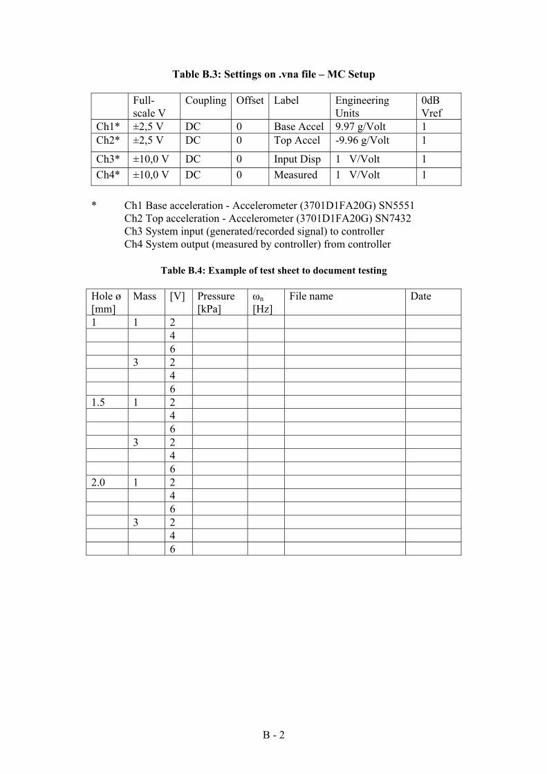
B - 2

Table B.3: Settings on .vna file – MC Setup Full-

scale V Coupling Offset Label Engineering

Units 0dB Vref

Ch1* ±2,5 V DC 0 Base Accel 9.97 g/Volt 1 Ch2* ±2,5 V DC 0 Top Accel -9.96 g/Volt 1

Ch3* ±10,0 V DC 0 Input Disp 1 V/Volt 1 Ch4* ±10,0 V DC 0 Measured 1 V/Volt 1

* Ch1 Base acceleration - Accelerometer (3701D1FA20G) SN5551 Ch2 Top acceleration - Accelerometer (3701D1FA20G) SN7432 Ch3 System input (generated/recorded signal) to controller Ch4 System output (measured by controller) from controller

Table B.4: Example of test sheet to document testing Hole ø [mm]

Mass [V] Pressure [kPa]

ωn [Hz]

File name Date

1 1 2 4 6 3 2 4 6 1.5 1 2 4 6 3 2 4 6 2.0 1 2 4 6 3 2 4 6

C - 1

Appendix C: Results

C.1 Air-spring simulation and test – load case 1, 1 - 3m/s2 r.m.s

0.5 1 1.5 2 2.5 3 3.5 4 4.5 5 5.5 60

0.5

1

1.5

2

2.5

3

3.5

4

4.5

Transfer function - air-springSimulation load case 1, 1 m/s2 r.m.s.

Frequency [Hz]

Tran

smis

sibi

lity

Linear Non-linear Complex

0.5 1 1.5 2 2.5 3 3.5 4 4.5 5 5.5 60

0.5

1

1.5

2

2.5

3

3.5

4

4.5

Transfer function - air-springSimulation and experiment load case 1, 1 m/s2 r.m.s.

Frequency [Hz]

Tran

smis

sibi

lity

Linear Non-linear Complex Experiment

C - 2

0.5 1 1.5 2 2.5 3 3.5 4 4.5 5 5.5 60

0.5

1

1.5

2

2.5

3

3.5

4

4.5

Transfer function - air-springSimulation load case 1, 2 m/s2 r.m.s.

Frequency [Hz]

Tran

smis

sibi

lity

Linear Non-linear Complex

0.5 1 1.5 2 2.5 3 3.5 4 4.5 5 5.5 60

0.5

1

1.5

2

2.5

3

3.5

4

4.5

Transfer function - air-springSimulation and experiment load case 1, 2 m/s2 r.m.s.

Frequency [Hz]

Tran

smis

sibi

lity

Linear Non-linear Complex Experiment

C - 3

0.5 1 1.5 2 2.5 3 3.5 4 4.5 5 5.5 60

0.5

1

1.5

2

2.5

3

3.5

4

4.5

Transfer function - air-springSimulation load case 1, 3 m/s2 r.m.s.

Frequency [Hz]

Tran

smis

sibi

lity

Linear Non-linear Complex

0.5 1 1.5 2 2.5 3 3.5 4 4.5 5 5.5 60

0.5

1

1.5

2

2.5

3

3.5

4

4.5

5

Transfer function - air-springSimulation and experiment load case 1, 3 m/s2 r.m.s.

Frequency [Hz]

Tran

smis

sibi

lity

Linear Non-linear Complex Experiment

C - 4

C.2 Air-spring simulation and test – load case 2, 1 - 3m/s2 r.m.s.

0.5 1 1.5 2 2.5 3 3.5 4 4.5 5 5.5 60

0.5

1

1.5

2

2.5

3

3.5

4

4.5

5

Transfer function - air-springSimulation load case 2, 1 m/s2 r.m.s.

Frequency [Hz]

Tran

smis

sibi

lity

Linear Non-linear Complex

0.5 1 1.5 2 2.5 3 3.5 4 4.5 5 5.5 60

0.5

1

1.5

2

2.5

3

3.5

4

4.5

5

Transfer function - air-springSimulation and experiment load case 2, 1 m/s2 r.m.s.

Frequency [Hz]

Tran

smis

sibi

lity

Linear Non-linear Complex Experiment

C - 5

0.5 1 1.5 2 2.5 3 3.5 4 4.5 5 5.5 60

0.5

1

1.5

2

2.5

3

3.5

4

4.5

5

Transfer function - air-springSimulation load case 2, 2 m/s2 r.m.s.

Frequency [Hz]

Tran

smis

sibi

lity

Linear Non-linear Complex

0.5 1 1.5 2 2.5 3 3.5 4 4.5 5 5.5 60

0.5

1

1.5

2

2.5

3

3.5

4

4.5

5

5.5

Transfer function - air-springSimulation and experiment load case 2, 2 m/s2 r.m.s.

Frequency [Hz]

Tran

smis

sibi

lity

Linear Non-linear Complex Experiment

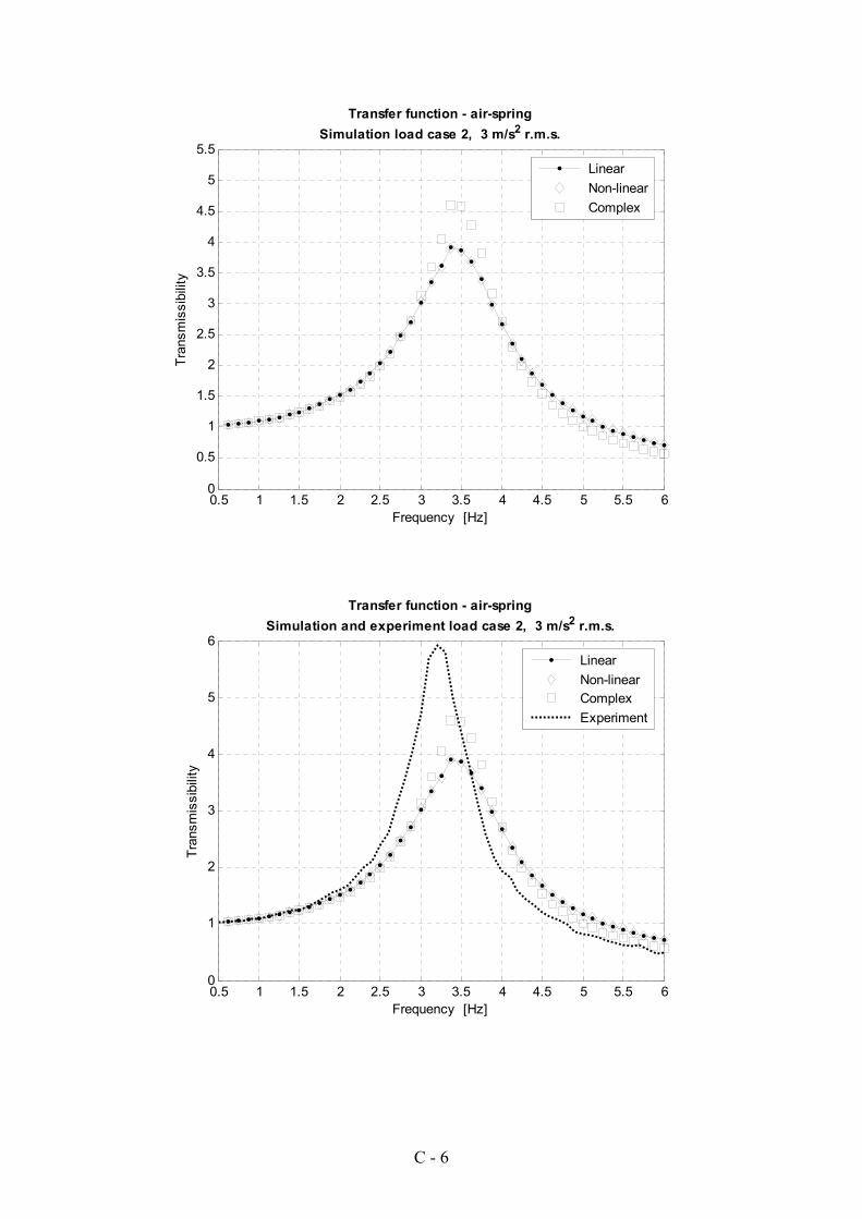
C - 6

0.5 1 1.5 2 2.5 3 3.5 4 4.5 5 5.5 60

0.5

1

1.5

2

2.5

3

3.5

4

4.5

5

5.5

Transfer function - air-springSimulation load case 2, 3 m/s2 r.m.s.

Frequency [Hz]

Tran

smis

sibi

lity

Linear Non-linear Complex

0.5 1 1.5 2 2.5 3 3.5 4 4.5 5 5.5 60

1

2

3

4

5

6

Transfer function - air-springSimulation and experiment load case 2, 3 m/s2 r.m.s.

Frequency [Hz]

Tran

smis

sibi

lity

Linear Non-linear Complex Experiment

C - 7

C.3 Air-spring simulation and test – load case 3, 1 - 3m/s2 r.m.s.

0.5 1 1.5 2 2.5 3 3.5 4 4.5 5 5.5 60

0.5

1

1.5

2

2.5

3

3.5

4

4.5

5

5.5

Transfer function - air-springSimulation load case 3, 1 m/s2 r.m.s.

Frequency [Hz]

Tran

smis

sibi

lity

Linear Non-linear Complex

0.5 1 1.5 2 2.5 3 3.5 4 4.5 5 5.5 60

0.5

1

1.5

2

2.5

3

3.5

4

4.5

5

5.5

Transfer function - air-springSimulation and experiment load case 3, 1 m/s2 r.m.s.

Frequency [Hz]

Tran

smis

sibi

lity

Linear Non-linear Complex Experiment

C - 8

0.5 1 1.5 2 2.5 3 3.5 4 4.5 5 5.5 60

0.5

1

1.5

2

2.5

3

3.5

4

4.5

5

5.5

Transfer function - air-springSimulation load case 3, 2 m/s2 r.m.s.

Frequency [Hz]

Tran

smis

sibi

lity

Linear Non-linear Complex

0.5 1 1.5 2 2.5 3 3.5 4 4.5 5 5.5 60

0.5

1

1.5

2

2.5

3

3.5

4

4.5

5

5.5

Transfer function - air-springSimulation and experiment load case 3, 2 m/s2 r.m.s.

Frequency [Hz]

Tran

smis

sibi

lity

Linear Non-linear Complex Experiment

C - 9

0.5 1 1.5 2 2.5 3 3.5 4 4.5 5 5.5 60

0.5

1

1.5

2

2.5

3

3.5

4

4.5

5

5.5

Transfer function - air-springSimulation load case 3, 3 m/s2 r.m.s.

Frequency [Hz]

Tran

smis

sibi

lity

Linear Non-linear Complex

0.5 1 1.5 2 2.5 3 3.5 4 4.5 5 5.5 60

1

2

3

4

5

6

Transfer function - air-springSimulation and experiment load case 3, 3 m/s2 r.m.s.

Frequency [Hz]

Tran

smis

sibi

lity

Linear Non-linear Complex Experiment

C - 10

C.4 Air-spring simulation and test – load case 4, 1 - 3m/s2 r.m.s.

0.5 1 1.5 2 2.5 3 3.5 4 4.5 5 5.5 60

0.5

1

1.5

2

2.5

3

3.5

4

4.5

5

5.5

Transfer function - air-springSimulation load case 4, 1 m/s2 r.m.s.

Frequency [Hz]

Tran

smis

sibi

lity

Linear Non-linear Complex

0.5 1 1.5 2 2.5 3 3.5 4 4.5 5 5.5 60

0.5

1

1.5

2

2.5

3

3.5

4

4.5

5

5.5

Transfer function - air-springSimulation and experiment load case 4, 1 m/s2 r.m.s.

Frequency [Hz]

Tran

smis

sibi

lity

Linear Non-linear Complex Experiment

C - 11

0.5 1 1.5 2 2.5 3 3.5 4 4.5 5 5.5 60

0.5

1

1.5

2

2.5

3

3.5

4

4.5

5

5.5

Transfer function - air-springSimulation load case 4, 2 m/s2 r.m.s.

Frequency [Hz]

Tran

smis

sibi

lity

Linear Non-linear Complex

0.5 1 1.5 2 2.5 3 3.5 4 4.5 5 5.5 60

1

2

3

4

5

6

Transfer function - air-springSimulation and experiment load case 4, 2 m/s2 r.m.s.

Frequency [Hz]

Tran

smis

sibi

lity

Linear Non-linear Complex Experiment

C - 12

0.5 1 1.5 2 2.5 3 3.5 4 4.5 5 5.5 60

0.5

1

1.5

2

2.5

3

3.5

4

4.5

5

5.5

Transfer function - air-springSimulation load case 4, 3 m/s2 r.m.s.

Frequency [Hz]

Tran

smis

sibi

lity

Linear Non-linear Complex

0.5 1 1.5 2 2.5 3 3.5 4 4.5 5 5.5 60

1

2

3

4

5

6

7

Transfer function - air-springSimulation and experiment load case 4, 3 m/s2 r.m.s.

Frequency [Hz]

Tran

smis

sibi

lity

Linear Non-linear Complex Experiment

C - 13

C.5 Air-spring and auxiliary volume simulation and test – load case 1, 1 - 3m/s2 r.m.s.

0.5 1 1.5 2 2.5 3 3.5 4 4.5 5 5.5 60

0.5

1

1.5

2

2.5

3

3.5

Transfer Function - air-spring and aux. volumeSimulation load case 1, 1 m/s2 r.m.s.

Frequency [Hz]

Tran

smis

sibi

lity

∅ 1.0 mm ∅ 1.5 mm ∅ 2.0 mm ∅ 2.5 mm ∅ 3.5 mm

0.5 1 1.5 2 2.5 3 3.5 4 4.5 5 5.5 60

0.5

1

1.5

2

2.5

3

3.5

4

4.5

Transfer Function - air-spring and aux. volumeSimulation and experiment load case 1, 1 m/s2 r.m.s.

Frequency [Hz]

Tran

smis

sibi

lity

∅ 1.0 mm (sim) ∅ 2.5 mm (sim) ∅ 6.5 mm (sim) ∅ 1.0 mm (exp) ∅ 2.5 mm (exp)

C - 14

0.5 1 1.5 2 2.5 3 3.5 4 4.5 5 5.5 60

0.5

1

1.5

2

2.5

3

3.5

4

Transfer Function - air-spring and aux. volumeSimulation load case 1, 2 m/s2 r.m.s.

Frequency [Hz]

Tran

smis

sibi

lity

∅ 1.0 mm ∅ 1.5 mm ∅ 2.0 mm ∅ 2.5 mm ∅ 3.5 mm

0.5 1 1.5 2 2.5 3 3.5 4 4.5 5 5.5 60

0.5

1

1.5

2

2.5

3

3.5

4

4.5

Transfer Function - air-spring and aux. volumeSimulation and experiment load case 1, 2 m/s2 r.m.s.

Frequency [Hz]

Tran

smis

sibi

lity

∅ 1.0 mm (sim) ∅ 2.5 mm (sim) ∅ 5.5 mm (sim) ∅ 1.0 mm (exp) ∅ 2.5 mm (exp) ∅ 6.5 mm (exp)

C - 15

0.5 1 1.5 2 2.5 3 3.5 4 4.5 5 5.5 60

0.5

1

1.5

2

2.5

3

3.5

4

Transfer Function - air-spring and aux. volumeSimulation load case 1, 3 m/s2 r.m.s.

Frequency [Hz]

Tran

smis

sibi

lity

∅ 1.0 mm ∅ 1.5 mm ∅ 2.0 mm ∅ 2.5 mm ∅ 3.5 mm

0.5 1 1.5 2 2.5 3 3.5 4 4.5 5 5.5 60

0.5

1

1.5

2

2.5

3

3.5

4

4.5

Transfer Function - air-spring and aux. volumeSimulation and experiment load case 1, 3 m/s2 r.m.s.

Frequency [Hz]

Tran

smis

sibi

lity

∅ 1.0 mm (sim) ∅ 2.5 mm (sim) ∅ 5.5 mm (sim) ∅ 1.0 mm (exp) ∅ 2.5 mm (exp) ∅ 6.5 mm (exp)

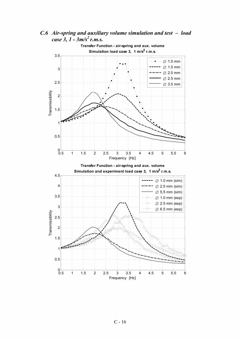
C - 16

C.6 Air-spring and auxiliary volume simulation and test – load case 3, 1 - 3m/s2 r.m.s.

0.5 1 1.5 2 2.5 3 3.5 4 4.5 5 5.5 60

0.5

1

1.5

2

2.5

3

3.5

Transfer Function - air-spring and aux. volumeSimulation load case 3, 1 m/s2 r.m.s.

Frequency [Hz]

Tran

smis

sibi

lity

∅ 1.0 mm ∅ 1.5 mm ∅ 2.0 mm ∅ 2.5 mm ∅ 3.5 mm

0.5 1 1.5 2 2.5 3 3.5 4 4.5 5 5.5 60

0.5

1

1.5

2

2.5

3

3.5

4

4.5

Transfer Function - air-spring and aux. volumeSimulation and experiment load case 3, 1 m/s2 r.m.s.

Frequency [Hz]

Tran

smis

sibi

lity

∅ 1.0 mm (sim) ∅ 2.5 mm (sim) ∅ 5.5 mm (sim) ∅ 1.0 mm (exp) ∅ 2.5 mm (exp) ∅ 6.5 mm (exp)

C - 17

0.5 1 1.5 2 2.5 3 3.5 4 4.5 5 5.5 60

0.5

1

1.5

2

2.5

3

3.5

4

Transfer Function - air-spring and aux. volumeSimulation load case 3, 2 m/s2 r.m.s.

Frequency [Hz]

Tran

smis

sibi

lity

∅ 1.0 mm ∅ 1.5 mm ∅ 2.0 mm ∅ 2.5 mm ∅ 3.5 mm

0.5 1 1.5 2 2.5 3 3.5 4 4.5 5 5.5 60

0.5

1

1.5

2

2.5

3

3.5

4

4.5

Transfer Function - air-spring and aux. volumeSimulation and experiment load case 3, 2 m/s2 r.m.s.

Frequency [Hz]

Tran

smis

sibi

lity

∅ 1.0 mm (sim) ∅ 2.5 mm (sim) ∅ 5.5 mm (sim) ∅ 1.0 mm (exp) ∅ 2.5 mm (exp) ∅ 6.5 mm (exp)

C - 18

0.5 1 1.5 2 2.5 3 3.5 4 4.5 5 5.5 60

0.5

1

1.5

2

2.5

3

3.5

4

Transfer Function - air-spring and aux. volumeSimulation load case 3, 3 m/s2 r.m.s.

Frequency [Hz]

Tran

smis

sibi

lity

∅ 1.0 mm ∅ 1.5 mm ∅ 2.0 mm ∅ 2.5 mm ∅ 3.5 mm

0.5 1 1.5 2 2.5 3 3.5 4 4.5 5 5.5 60

0.5

1

1.5

2

2.5

3

3.5

4

4.5

Transfer Function - air-spring and aux. volumeSimulation and experiment load case 3, 3 m/s2 r.m.s.

Frequency [Hz]

Tran

smis

sibi

lity

∅ 1.0 mm (sim) ∅ 2.5 mm (sim) ∅ 5.5 mm (sim) ∅ 1.0 mm (exp) ∅ 2.5 mm (exp) ∅ 6.5 mm (exp)

C - 19

0.5 1 1.5 2 2.5 3 3.5 4 4.5 5 5.5 60

0.5

1

1.5

2

2.5

3

3.5

4

Transfer Function - air-spring and aux. volume V/3Simulation load case 3, 3 m/s2 r.m.s.

Frequency [Hz]

Tran

smis

sibi

lity

∅ 1.0 mm ∅ 1.5 mm ∅ 2.0 mm ∅ 2.5 mm ∅ 3.5 mm