Embed Size (px)
Citation preview

BIS Working Papers No 230
Modelling and calibration errors in measures of portfolio credit risk by Nikola Tarashev and Haibin Zhu
Monetary and Economic Department June 2007
Abstract This paper develops an empirical procedure for analyzing the impact of model misspecification and calibration errors on measures of portfolio credit risk. When applied to large simulated portfolios with realistic characteristics, this procedure reveals that violations of key assumptions of the well-known Asymptotic Single-Risk Factor (ASRF) model are virtually inconsequential. By contrast, flaws in the calibrated interdependence of credit risk across exposures, which are driven by plausible small-sample estimation errors or popular rule-of-thumb values of asset return correlations, can lead to significant inaccuracies in measures of portfolio credit risk. Similar inaccuracies arise under erroneous, albeit standard, assumptions regarding the tails of the distribution of asset returns. JEL Classification Numbers: G21, G28, G13, C15. Keywords: Correlated defaults, value at risk, multiple common factors, granularity, estimation error, tail dependence, bank capital.

BIS Working Papers are written by members of the Monetary and Economic Department of the Bank for International Settlements, and from time to time by other economists, and are published by the Bank. The views expressed in them are those of their authors and not necessarily the views of the BIS.
Copies of publications are available from:
Bank for International Settlements Press & Communications CH-4002 Basel, Switzerland E-mail: [email protected]
Fax: +41 61 280 9100 and +41 61 280 8100
This publication is available on the BIS website (www.bis.org).
© Bank for International Settlements 2007. All rights reserved. Limited extracts may be reproduced or translated provided the source is stated.
ISSN 1020-0959 (print)
ISSN 1682-7678 (online)
Modelling and Calibration Errors in Measures of
Portfolio Credit Risk∗
Nikola Tarashev†
Haibin Zhu‡
June 2007
Abstract
This paper develops an empirical procedure for analyzing the impact of modelmisspecification and calibration errors on measures of portfolio credit risk. Whenapplied to large simulated portfolios with realistic characteristics, this procedure revealsthat violations of key assumptions of the well-known Asymptotic Single-Risk Factor(ASRF) model are virtually inconsequential. By contrast, flaws in the calibrated inter-dependence of credit risk across exposures, which are driven by plausible small-sampleestimation errors or popular rule-of-thumb values of asset return correlations, can leadto significant inaccuracies in measures of portfolio credit risk. Similar inaccuracies ariseunder erroneous, albeit standard, assumptions regarding the tails of the distributionof asset returns.
JEL Classification Numbers: G21, G28, G13, C15Keywords: Correlated defaults; Value at risk; Multiple common factors; Granularity;Estimation error; Tail dependence; Bank capital
∗We are indebted to Michael Gordy and Kostas Tsatsaronis for their encouragement and useful commentson an earlier version of this paper. We thank Klaus Duellmann, Wenying Jiangli, and participants at a BISworkshop, the 3rd International Conference on Credit and Operational Risk at HEC Montreal and the 17th
Annual Derivatives Securities and Risk Management Conference at the FDIC for insightful suggestions. Weare also grateful to Marcus Jellinghaus for his valuable help with the data. The views expressed in this paperare our own and do not necessarily represent those of the Bank for International Settlements.
†Nikola Tarashev: Research and Policy Analysis, Bank for International Settlements, Basel, Switzerland.Tel.: 41-61-280-9213. Fax: 41-61-280-9100. E-mail: [email protected].
‡Haibin Zhu: Research and Policy Analysis, Bank for International Settlements, Basel, Switzerland. Tel.:41-61-280-9164. Fax: 41-61-280-9100. E-mail: [email protected].

Modelling and Calibration Errors in Measures of Portfolio Credit Risk
Abstract
This paper develops an empirical procedure for analyzing the impact of model misspec-ification and calibration errors on measures of portfolio credit risk. When applied to largesimulated portfolios with realistic characteristics, this procedure reveals that violations ofkey assumptions of the well-known Asymptotic Single-Risk Factor (ASRF) model are vir-tually inconsequential. By contrast, flaws in the calibrated inter-dependence of credit riskacross exposures, which are driven by plausible small-sample estimation errors or popularrule-of-thumb values of asset return correlations, can lead to significant inaccuracies in mea-sures of portfolio credit risk. Similar inaccuracies arise under erroneous, albeit standard,assumptions regarding the tails of the distribution of asset returns.
JEL Classification Numbers: G21, G28, G13, C15Keywords: Correlated defaults; Value at risk; Multiple common factors; Granularity; Es-timation error; Tail dependence; Bank capital
1 Introduction
Assessments of portfolio credit risk, which are often based on analytical models, have at-
tracted much attention in recent years. One reason is that participants in the increas-
ingly popular market for structured finance products rely heavily on estimates of the inter-
dependence of credit risk across various exposures.1 Such estimates are also of principal
interest to financial supervisors who, in enforcing new standards in the banking and insur-
ance industries, have to ensure that regulatory capital is closely aligned with credit risk.
This paper investigates the well-known Asymptotic Single-Risk Factor (ASRF) model
of portfolio credit risk. The popularity of this model stems from its implication that the
contribution of each exposure to the credit value-at-risk (VaR) of the portfolio – defined as
the maximum default loss that can be incurred with a given probability over a given horizon
– is independent of the characteristics of the other exposures. This implication – which has
been derived rigorously in Gordy (2003) and is known as portfolio invariance of marginal
credit VaR contributions – underpins the internal-ratings-based (IRB) approach of the Basel
II framework (BCBS, 2005). The implication has been interpreted as alleviating the data
requirements and computational burden on users of the model. Indeed, portfolio invariance
implies that credit VaR can be calculated solely on the basis of exposure-specific parameters,
including individual probability of default (PD), loss-given-default (LGD) and dependence
on the common factor.
Its popularity notwithstanding, the “portfolio invariance” implication of the ASRF model
hinges on two strong assumptions that have been criticized as sources of misspecification
errors. Namely, the model assumes that the systematic component of credit risk is governed
by a single common factor and that the portfolio is so finely grained that all idiosyncratic risks
are diversified away. Violations of the “single-factor” and “perfect granularity” assumptions
would translate directly into erroneous assessments of portfolio credit risk.
Moreover, an application of the ASRF model may be quite challenging, even if this model
is well specified. An important reason is that the portfolio invariance implication does not
exempt a user of the model from adopting a global approach. In particular, estimates of
exposure-specific dependence on the common factor, which are required for a calibration
of the ASRF model, hinge on information about the correlation structure in the portfolio
1Examples of structured finance products are collateralized debt obligations (CDOs), nth-to-default creditdefault swaps (CDSs) and CDS indices.
1
or about the common factor itself.2 When such portfolio- or market-wide information is
imperfect, the user will implement a flawed calibration of the model, which will be another
source of errors in measured portfolio credit risk.
A contribution of this paper is to develop a unified method for quantifying the im-
portance of model misspecification and calibration errors in assessments of portfolio credit
risk. In order to implement this method, we rely on a large data set that comprises Moody’s
KMV estimates of PDs and pairwise asset return correlations for nearly 11, 000 non-financial
corporates worldwide. We treat these estimates as the actual credit risk parameters of hy-
pothetical portfolios that match the industrial-sector concentration of typical portfolios of
US wholesale banks. For each such portfolio, we derive the “true” probability distribution of
default losses and then condense this distribution into unexpected losses, which are defined
as a credit VaR net of expected losses. This summary statistic is equivalent to a “target”
capital measure necessary to cover default losses with a desired probability.3 The target
capital measure can be compared directly to a “shortcut” capital measure, which is based
on the ASRF model and a rule-of-thumb calibration of exposure-specific dependence on a
single common factor.
We decompose the difference between the target and shortcut capital measures into four
non-overlapping and exhaustive components. Two of these components relate to the sources
of misspecification of the ASRF model discussed above and are attributed to a “multi-factor”
effect and a “granularity” effect, respectively. The other two components, which we derive
after transforming the correlation structure to be consistent with the ASRF model, relate to
errors in the calibration of the inter-dependence of credit risk across exposures.4 Specifically,
the calibration errors we consider arise either from an overall bias in the measured correlations
of firms’ asset returns – which gives rise to what we dub the “correlation level” effect – or from
noise in the measured dispersion of these correlations across pairs of firms – the “correlation
dispersion” effect.
Another contribution of this paper is that it provides two additional perspectives on flaws
in the calibration of the ASRF model. First, we calculate deviations from a desired capital
2The IRB capital formula of Basel II avoids the necessity of a global approach by postulating that firm-specific dependence on the single common factor is determined fully by the level of the corresponding PD.
3In this paper, we use the terms “assessment of credit risk” and “capital measure” interchangeably.Importantly, our capital measures do not correspond to “regulatory capital”, which reflects considerationsof bank supervisors, or to “economic capital”, which reflects additional strategic and business objectives offinancial firms.
4In order to sharpen the analysis, we do not analyse the implications of errors in the estimates of PDsand LGDs.
2
buffer that arise not from the adoption of rule-of-thumb parameter values but from plausible
small-sample errors in asset return correlation estimates. Second, motivated by the analysis
in Gordy (2000) and Frey and McNeil (2003), we examine the importance of errors in the
calibrated tail dependence among individual asset return distributions. The impact of such
errors on capital measures is similar to but separate from the impact of errors in estimated
asset return correlations.
Our main conclusion is that errors in the practical implementation, as opposed to the
specification, of the ASRF model are the main sources of potential miscalculations of the
credit risk in large portfolios. Specifically, the misspecification-driven multi-factor effect leads
a user of the model to underpredict target capital buffers by only 1%. This is because a single-
factor approximation, if chosen carefully, fits well the correlation structure of asset returns in
our data. Similarly, the granularity effect causes calculated capital to underpredict the target
level by 5%. By contrast, assessments of portfolio credit risk are considerably more sensitive
to possible miscalibrations of the single-factor model. The correlation dispersion effect, for
example, leads to capital measures that are 12% higher than the target level. In turn,
the correlation level effect makes calculated capital over(under)predict the target measure
by roughly 8% for each percentage point over(under)estimation of the average correlation
coefficient. Furthermore, plausible small-sample errors in correlation estimates – arising
when users of the model have 5 to 10 years of monthly asset returns data – translate into
capital measures that may deviate from the target level by 30 to 45%.5 Finally, data on asset
returns suggests that the empirical tail dependence among the underlying distributions is at
odds with the conventional multi-normality assumption. Concretely, a capital measure that
incorporates this assumption underestimates the target level by 22 to 86%.
Among the four effects on capital calculations, only the granularity effect is sensitive
to the number of exposures in the portfolio. When this number decreases, the portfolio
maintains a larger portion of idiosyncratic risks and, thus, we are not surprised to find
that the granularity effect leads to a 19% underestimation of target capital in typical small
portfolios.
In comparison to articles in the related literature, this paper covers a wider range of
errors in assessments of portfolio credit risk. Most of these articles have focused exclusively
5Of course, it is reasonable to expect that plausible small-sample estimation errors would have a significantimpact on capital measures based on any model of portfolio credit risk, irrespective of whether the modelaccommodates a single or multiple factors. We do not quantify such an impact, however, because doing sowould be a digression from the main focus of our analysis.
3
on misspecifications of the ASRF model and have proposed ways to partially correct for
them without impairing the model’s tractability. Empirical analyses of violations of the
perfect granularity assumption include Martin and Wilde (2002), Vasicek (2002), Emmer
and Tasche (2003), and Gordy and Luetkebohmert (2006). For their part, Pykhtin (2004),
Duellmann (2006), Garcia Cespedes et al. (2006) and Duellmann and Masschelein (2006a)
have analyzed implications of the common factor assumption under different degrees of
portfolio concentration in a limited number of industrial sectors. In addition, Heitfield et al.
(2006) and Duellman et al. (2006) have examined both granularity and sector concentration
issues in the context of US and European bank portfolios, respectively.6 A small branch
of the related literature, which includes Loeffler (2003) and Morinaga and Shiina (2005),
has analyzed calibration issues and has derived that noise in model parameters can have a
significant impact on assessments of portfolio credit risk.
The remainder of this paper is organized as follows. Section 2 outlines the ASRF model
and the empirical methodology applied to it. Section 3 describes the data and Section 4
reports the empirical results. Finally, Section 5 concludes.
2 Methodology
In this section, we first outline the ASRF model. Then, we discuss how violations of its
key assumptions or flawed calibration of its parameters can affect assessments of portfolio
credit risk. Finally, we develop an empirical methodology for quantifying and comparing
alternative sources of error in such assessments.
2.1 The ASRF model7
The ASRF model of portfolio credit risk – introduced by Vasicek (1991) – postulates that
an obligor defaults when the value of its assets falls below some threshold. In addition, the
model assumes that asset values are driven by a single common factor:
ViT = ρi · MT +√
1 − ρ2i · ZiT (1)
6The recent working paper by the Basel Committee on Bank Supervision (BCBS, 2006) provides anextensive review of these articles.
7This section provides an intuitive discussion of the ASRF model. For a rigorous and detailed study ofthis model, see Gordy (2003). In addition, Frey and McNeil (2003) examine the calibration of the ASRFmodel under the so-called Bernoulli mixture representation.
4
where: ViT is the value of assets of obligor i at time T ; MT and ZiT denote the common
and idiosyncratic factors, respectively; and ρi ∈ [−1, 1] is the obligor-specific loading on the
common factor. The common and idiosyncratic factors are independent of each other and
scaled to random variables with mean 0 and variance 1.8 Thus, the asset return correlation
between borrowers i and j is given by ρiρj .
The ASRF model delivers a closed-form approximation to the probability distribution of
default losses on a portfolio of N exposures. The accuracy of the approximation increases
when the number of exposures grows, N → ∞, and the largest exposure weight shrinks,
supi (wi) → 0. In these limits, as the portfolio becomes perfectly granular, the probability
distribution of default losses can be derived as follows. First, let the indicator IiT equal 1 if
obligor i is in default at time T and 0 otherwise. Conditional on the value of the common
factor, the expectation of the indicator equals
E(IiT |MT ) = Pr(ViT < F−1(PDiT )|MT )
= Pr(ρi · MT +√
1 − ρ2i · ZiT < F−1(PDiT )|MT )
= H(
F−1(PDiT ) − ρiMT√
1 − ρ2i
)
where: PDiT is the unconditional probability that obligor i is in default at time T ; the
cumulative distribution function (CDF) of ZiT is denoted by H(·); and the CDF of ViT is
F(·), implying that the default threshold equals F−1(PDiT ).
Second, under perfect granularity, the Law of Large Numbers implies that the conditional
total loss on the portfolio, TL|M , is deterministic for any value of the common factor M :
TL|M =∑
i
wi · E (LGDi) · E(Ii|M)
=∑
i
wi · E (LGDi) · H(
F−1(PDi) − ρiM√
1 − ρ2i
)
(2)
where time subscripts have been suppressed. In addition, the loss-given-default of obligor i,
LGDi , is assumed to be independent of both the common and idiosyncratic factors.9
8The ASRF model can accommodate distributions with infinite second moments. Nonetheless, we abstractfrom this generalization in order to streamline the analysis.
9The ASRF model does allow for inter-dependence between asset returns and the LGD random variable.Such inter-dependence leads to another dimension in the study of portfolio credit risk, which is explored byKupiec (2007). We abstract from this additional dimension in order to focus on the correlation of defaultevents.
5
Finally, the conditional total loss TL|M is a decreasing function of the common factor M
and, consequently, the unconditional distribution of TL can be derived directly on the basis
of equation (2) and the CDF of the common factor, G(·). Denoting by TL1−α the (1 − α)th
percentile in the distribution of total losses, i.e. Pr (TL < TL1−a) = 1 − α, it follows that:
TL1−α =∑
i
wi · E (LGDi) · H(
F−1(PDi) − ρiG−1(α)√
1 − ρ2i
)
(3)
= TL|Mα
where Mα is the αth percentile in the distribution of the common factor. The magnitude
TL1−α is also known as the credit VaR at the (1 − α) confidence level.
Thus, in order to cover unexpected (i.e. total minus expected) losses with probability
(1 − α), the capital buffer for the entire portfolio should be set to:
κ = TL1−α −∑
i
wi · E (LGDi) · PDi
=∑
i
wi · E (LGDi) · [H(
F−1(PDi) − ρiG−1(α)√
1 − ρ2i
)
− PDi] (4)
≡∑
i
wi · κi
As implied by this equation, the capital buffer for the portfolio can be set on the basis of
exposure-specific parameters. These parameters reflect the weight of a given exposure in the
portfolio, the exposure’s LGD and PD as well as the underlying dependence on the common
factor. The flip side of this implication is that each exposure-specific portion of the capital
buffer is independent of the rest of the portfolio and, thus, is portfolio invariant.
In practice, an implementation of the ASRF model requires that one specify the distri-
bution of the common and idiosyncratic factors of asset returns. It is standard to assume
normal distributions and rewrite equation (4) as:
κ =∑
i
wi · E (LGDi) · [Φ(
Φ−1(PDi) − ρiΦ−1(α)
√
1 − ρ2i
)
− PDi] (5)
where Φ(·) is the CDF of a standard normal variable. Notice that equation (5) underpins
the regulatory capital formula in the IRB approach of Basel II, in which LGD is set to be
45% and α is chosen as 0.1%.
6
2.2 Impact of model misspecification
The portfolio invariance implication of the ASRF model hinges on two key assumptions, i.e.
that the portfolio is of perfect granularity and that there is a single common factor. In the
light of this, we examine at a conceptual level how violations of either of these assumptions
– which give rise to “granularity” and “multi-factor” effects – affect capital measures. For
the illustrative examples in this section, we use the ASRF formula in equation (5) and set
α = 0.1%.
2.2.1 Granularity effect
The granularity effect arises empirically either because of a limited number of exposures or
because of exposure concentration in a small number of borrowers. In either of these cases,
idiosyncratic risk is not fully diversified away. Therefore, the existence of a granularity
effect implies that capital measures based on the ASRF model would be insufficient to cover
unexpected losses.
The top-left panel in Figure 1 provides an illustrative example of the granularity effect. In
this example, the desired capital level for a homogenous portfolio is computed as a function of
the number of exposures (solid line).10 In addition, the figure also plots the capital measure
implied by the ASRF model (dotted line), which differs from the target one only in that it
assumes an infinite number of exposures. The difference between the dotted and solid lines
equals the magnitude of the granularity effect. As expected, the granularity effect is always
negative and decreases when the number of exposures increases.
Gordy and Luetkebohmert (2006) derive a closed-form “granularity adjustment”, which
should approximate the negative of the granularity effect. When the portfolio is homoge-
neous, the approximation is linear in the reciprocal of the number of exposures, which is
largely in line with the properties of the granularity effect plotted in Figure 1.11
2.2.2 Multi-factor effect
The impact of various macroeconomic and industry-specific conditions on portfolio credit
risk may be best accounted for by generalizing equation (1) in order to incorporate multiple
(potentially unobservable) common factors. Multiple common factors affect the likelihood
10The calculation of the desired capital level uses a Gaussian copula (see Appendix A).11Further comparison between the granularity effect and the granularity adjustment of Gordy and Luetke-
bohmert (2006) is reported in Section 4.1 below.
7
of default clustering – i.e. the likelihood of a large number of defaults occurring over a given
horizon – which influences the tails of the probability distribution of credit losses. In line
with our empirical results (reported in Section 4), our conceptual analysis treats a fattening
of these tails as implying unambiguously a higher level of the desired capital buffer.12
The existence of multiple common factors of credit risk violates the single-factor assump-
tion of the ASRF model, leading to what we call a multi-factor effect in capital measures.
Depending on the characteristics of the credit portfolio, the multi-factor effect could be ei-
ther negative – i.e. implying that the ASRF model underestimates the desired capital – or
positive. To illustrate the two possibilities, we generalize equation (1):
Vi = ρ1,i · M1 + ρ2,i · M2 +√
1 − ρ21,i − ρ2
2,i · Zi (6)
assuming that M1, M2 and Z are mutually independent standard normal variables.
In our first example, we consider a portfolio in which all exposures have equal weights,
have the same PD and are divided into two groups according to their dependence on the
common factors. For exposures in the first group, 0 < ρ1,i = ρ < 1 and ρ2,i = 0; while ρ1,j = 0
and 0 < ρ2,j = ρ < 1 for exposures in the second group. Thus, the common factors are group
specific and underpin positive and homogeneous within-group pairwise correlations and zero
across-group correlations. The solid line in the top-right panel of Figure 1 plots the desired
capital measure for such a portfolio as a function of the relative weight of exposures in group
1.13 This measure is lowest when the portfolio is most diversified between the two groups
of exposures and, thus, the probability of large default losses is minimized. In addition, the
dashed line in the figure plots an alternative capital measure, which is based on the ASRF
model and is underpinned by a single-factor structure of the asset return correlations. This
structure, which allows for providing the ASRF model with as much information about the
true correlations as possible (see Appendix C), turns out to match extremely well the true
average asset return correlation but to approximate only roughly the dispersion of correlation
coefficients in the cross section of exposures.
The difference between the dashed and solid lines equals the multi-factor effect. This
effect is negative because the single-factor assumption of the ASRF model ignores the fact
12Note that, depending on the confidence level of the targeted credit VaR, a fattening of the tails of theprobability distribution of credit losses may either raise or lower the desired capital buffer. Ceteris paribus,fatter tails of the loss distribution translate into a higher desired level of the capital buffer if the value of α
in equation (4) is sufficiently close to zero.13The desired capital buffer is calculated on the basis of Monte Carlo simulations (see Appendix B) for a
portfolio consisting of 1000 exposures.
8
that the common factors are two independent sources of default clustering, which leads to an
underestimation of the desired capital. The underestimation is largest when the two groups
enter the portfolio with equal weights, in which case the role of multiple factors is greatest.
It is possible, however, to construct another example, in which imposing an erroneous
single-factor structure on portfolio credit risk distorts the interaction between asset return
correlations and individual PDs in a way that leads to a positive multi-factor effect. Consider
a portfolio comprising two groups of exposures, with the exposures in the first group being
individually riskier but less correlated among themselves than the exposures in the second
group. In terms of equation (6), this can be formalized by postulating that firms with
high PDs feature 0 < ρ1,i = ρ < 1 and ρ2,i = 0, whereas firms with low PDs feature
0 < ρ1,j = ρ2,j = ρ < 1. A single-factor approximation to this correlation structure would
match the average correlation coefficient but would also imply too high a correlation among
riskier exposures. This could raise the probability of default clustering, suggesting a capital
buffer that is larger than desired.14
2.3 Impact of calibration errors
Errors in the calibration of the ASRF model will affect assessments of portfolio credit risk
even if this model is well specified. In this paper, we focus on errors in the calibration of the
inter-dependence of credit risk across exposures, which can be driven by noise in the adopted
values of asset return correlations or by a flawed assumption regarding the distribution of
asset returns. When analyzing the consequences of such errors, we maintain our earlier
practice and treat fattening of the tails of the loss distribution as implying unambiguously a
higher 99.9% credit VaR and, thus, a higher desired level of the capital buffer. In this way,
we sharpen the conceptual analysis and keep it in line with our empirical findings.
We study two general types of errors in calibrated asset return correlations: errors in the
average correlation coefficient and errors in the dispersion of correlation coefficients across
exposure pairs. Each error type is trivially independent of the granularity effect. In addition,
extracting the multi-factor effect on the basis of the single-factor approximation described
in Section 2.2.2 allows us to separate this effect from errors in the average correlation. By
contrast, errors in the calibrated dispersion of asset return correlations could arise either as
a result of imposing a single-factor structure on the correlation matrix in the presence of
14A similar result emerges when the dispersion of correlation coefficients is distorted and the true corre-lation structure is driven by a single common factor. In order to avoid overburdening of the exposition, weprovide a graphical illustration only in the single-factor context (see Section 2.3 below).
9

multiple factors (recall Section 2.2.2) or as a result of noise in the estimated factor loadings
when there is a single common factor. In this section, we are concerned with the second
case, as it is consistent with a correct specification of the ASRF model and refers only to
calibration errors.
The two types of errors in calibrated asset return correlations have various potential
sources. One possibility is that a user of the ASRF model is data constrained and, hence,
relies on rule-of-thumb values, which may simply be correlation estimates for popular credit
indices. Such estimates will lead to a discrepancy between desired and calculated capital
to the extent that the underlying indices are not representative of the user’s own portfolio.
Alternatively, a user of the model may have insufficient data on the assets of the obligors in
the portfolio, which would lead to small-sample estimation errors in asset return correlations.
Indeed, limitations on the availability of data points are likely to be important in practice
because: (i) asset value estimates are typically available at low (i.e. monthly or quarterly)
frequencies and (ii) supervisory texts require that financial institutions possess only five years
of relevant data.15
A positive error in the average level of asset return correlations leads to a capital measure
that is higher than the desired one (Figure 1, bottom-left panel). This result reflects the
intuition that inflating asset return correlations increases the likelihood of default clustering,
which fattens the tails of the loss distribution. In the remainder of this paper, the implication
of such errors is dubbed the “correlation level” effect.
In turn, the effect of noise in the estimated dispersion of correlation coefficients can be
seen in the following example. Suppose that all firms in one portfolio have homogeneous PDs
and exhibit homogeneous pairwise asset return correlations. Suppose further that a second
portfolio is characterized by the same PDs and average asset return correlation but includes
a group of firms that are more likely to default together. The second portfolio, in which
pairwise correlations exhibit dispersion, is more likely to experience several simultaneous
defaults and, thus, has a loss distribution with fatter tails. Consequently, between the two
portfolios, the second one requires higher capital in order to attain solvency with the same
probability. This is portrayed by the upward slope of the solid line in the bottom-right panel
of Figure 1 and is a particular instance of what we dub the “correlation dispersion” effect,
which arises in the context of a single common factor.
15Data limitations are likely to be important irrespective of how a user of the model estimates asset returncorrelations. Such estimates may rely on balance sheet information and stock market data. Alternatively,as derived in Tarashev and Zhu (2006), asset return correlations can be extracted from the CDS market.
10
This result can be strengthened (dashed line in the same panel) but also weakened or even
reversed if PDs vary across firms. To see why, consider the previous example but suppose
that the strongly correlated firms in the second portfolio are the ones that have the lowest
individual PDs. In other words, the firms that are likely to generate multiple defaults are
less likely to default. As a result, greater dispersion of asset return correlations may lower
the probability of default clustering in the second portfolio to an extent that depresses the
desired capital level below that for the first portfolio. This is illustrated by the negative
slope of the dotted line in the bottom-right panel of Figure 1.
Even if asset return correlations were known with certainty, a flawed calibration of
the marginal distributions of asset returns would still drive errors in the calibrated inter-
dependence of credit risk across exposures. Although the ASRF model imposes quite weak
restrictions on asset return distributions, it is common practice to adopt distributions whose
main advantages stem not from realistic features but from operational convenience. In par-
ticular, the consensus view in the literature is that asset returns have fatter tails than those
imposed by the conventional normality assumption. To the extent that this fatness of the
tails reflects the distribution of the common factor, the probability of default clustering and,
thus, the desired capital level would be higher than those derived under normality (Hull
and White, 2004; Tarashev and Zhu, 2006). We study this issue by considering Student-t
distributions for both the common and idiosyncratic factors of asset returns.
2.4 Evaluating various sources of error
An important contribution of this paper is to present a unified empirical method for quanti-
fying the impact of several sources of error in model-based assessment of portfolio credit risk.
In particular, we focus on the difference between target capital measures and shortcut ones,
the latter of which are based on the ASRF model and possible erroneous calibration of its
parameters. We dissect this difference into four non-overlapping and exhaustive components,
attributing them to the multi-factor, granularity, correlation level and correlation dispersion
effects. In order to probe further the likely magnitude of the last two effects, we derive
plausible small-sample errors that could affect direct estimates of asset return correlations.
Finally, we also examine the implications of erroneous assumptions regarding the marginal
distribution of asset returns.
The basic empirical method consists of two general steps. In the first step, we construct
a hypothetical portfolio that is either “large” – consisting of 1,000 equal exposures – or
11
“small” – consisting of 200 equal exposures.16 The sectoral composition of such a portfolio is
designed to be in line with the typical loan portfolio of large wholesale banks in the United
States.17 Given the constraints of such a composition, the portfolio is drawn at random from
our sample of firms. Since each simulated portfolio is subject to sampling noise, we examine
3,000 different draws for both large and small portfolios.
For a portfolio constructed in the first step, the second step calculates five alternative
capital measures, which differ in the underlying assumptions regarding the inter-dependence
of credit risk across exposures. Each of these alternatives employs the same set of PD values
and assumes that asset returns are normally distributed. In addition, each alternative is
based on the assumption that LGD is a random variable, which has a symmetric triangular
distribution that is identical across exposures, peaks at 50% and has a continuous support
on the interval [0%, 100%].18
Each measure differs from a previous one owing to a single assumption:
1. The target capital measure incorporates data on asset return correlations, which are
treated as representing the “truth”. Using these correlations, we conduct Monte Carlo
simulations to construct the “true” probability distribution of default losses at the
one-year horizon. The implied 99.9% credit VaR minus expected losses equals target
capital (see Appendix B for further detail).
2. The second capital measure differs from target capital only owing to a restriction on
the number of common factors governing asset returns. In particular, we adopt a
correlation matrix that fits the original one as closely as possible under the constraint
that correlation coefficients should be consistent with the presence of a single common
factor (see Appendix C). The fitted single-factor correlation matrix is used to derive
the one-year probability distribution of joint defaults on the basis of the so-called
16The distinction between what we dub large and small portfolios does not reflect the size of the aggregateexposure but rather different degrees of diversification across individual exposures. Importantly, the degreeof diversification in the large hypothetical portfolios studied in this paper matches the diversification inthe large real-world portfolios studied by Heitfield et al. (2006) (see Section 3.2). The small hypotheticalportfolios exhibit similar properties.
17Such a portfolio does not incorporate consumer loans and, thus, may not be representative of all aspectsof credit risk.
18The LGD specification warrants an explanation. The independence between the incidence of defaultsand LGDs implies that, in the absence of simulation noise, only the mean of the LGD distribution enters (asa multiplicative factor) capital measures. However, the entire LGD distribution affects measures obtainedfrom Monte Carlo simulations. Importantly, assuming a continuous distribution for LGDs smooths thederived probability distribution of joint defaults, which improves the robustness of simulation-based capitalmeasures.
12

Gaussian copula method (see Appendix A). This distribution is then mapped into a
probability distribution of default losses and, finally, into a capital measure.
3. The third capital measure differs from the second one only in that it assumes that
all idiosyncratic risk is diversified away. This assumption allows us to use the fitted
single-factor correlation matrix underpinning measure 2 in the ASRF formula (equation
5).
4. The fourth capital measure differs from the third one only in that it is based on the
assumption that loading coefficients on the single common factor are the same across
exposures. The resulting common correlation coefficient, which is set equal to the
average of the pairwise correlations underpinning measures 2 and 3, is used as an
input to the ASRF formula (equation 5).
5. Finally, the shortcut capital measure differs from the fourth one only in that it incor-
porates alternative, rule-of-thumb, values for the common correlation coefficient.
The three intermediate measures lead to a straightforward dissection of the difference
between target and shortcut capital.19 Specifically, the difference between measures 5 and
1 is the sum of the following four components: (i) the difference between measures 2 and
1, which equals the multi-factor effect; (ii) the difference between measures 3 and 2, which
equals the granularity effect; (iii) the difference between measures 4 and 3, which equals the
correlation dispersion effect; and (iv) the difference between measures 5 and 4, which equals
the correlation level effect.
The specific ordering and choice of the three intermediate capital measures is a result
of the following reasoning. As far as measure 2 is concerned, its position is fixed by the
necessity to extract the multi-factor effect first. The reason for this is twofold. First, deriving
a capital measure that assumes an infinite number of exposures but allows for multiple
factors (i.e. calculating measure 2 after the extraction of the granularity effect) is subject
to approximation errors (see Pykhtin, 2004, for example). Second, it is possible to isolate
calibration errors (via measures 3 and 4) only after the extraction of the multi-factor effect
(via measure 2) has modified the original correlation matrix to render it consistent with
the ASRF model. Likewise, an application of this model for the extraction of calibration
19Importantly, the method also applies to alternative definitions of target and short-cut capital, so longas the true correlation structure and short-cut correlation estimates chosen by the user are clearly defined.
13
errors requires the assumption of infinite granularity, which fixes the position of measure 3.20
Finally, modifying measure 4 by preserving the cross-sectional distribution of the single-
factor correlation coefficients but changing their average level would reverse the order in
which the correlation level and dispersion effects are extracted. An important problem with
this procedure is that it would allow only for an imperfect estimate of the correlation level
effect because this estimate would be influenced by changes in the structure of the single-
factor correlation matrix.
2.4.1 Two extensions
In an attempt to delve further into the impact of plausible calibration errors on capital
measures, we conduct two additional exercises. Each exercise focuses on a specific type of
errors in the calibrated inter-dependence of defaults and incorporates the assumption that
the true PDs are identical across exposures. This assumption insulates capital measures
from the impact of interaction between heterogeneous PDs and errors in the calibrated
inter-dependence of defaults.
In the first exercise, we derive the extent to which plausible limitations on the size of
available data can affect assessments of portfolio credit risk by affecting the estimates of asset
return correlations. Specifically, we draw time series of asset returns from a joint distribution
characterized by constant pairwise correlations equal to the correlation underpinning measure
4. Using the sample correlation matrix of the simulated series and a typical value for the
probability of default, we obtain an “estimated” capital measure on the basis of the ASRF
formula in equation 5.21 The difference between this measure and the desired capital, which
employs the exact correlation structure, are driven by small-sample noise in the estimates of
the overall level and dispersion of asset return correlations.
In our second exercise, we examine how measure 4 would change if the common and
idiosyncratic factors of asset returns are in fact driven by Student-t distributions. The results
of this exercise reveal how flawed calibration of the tail dependence among exposures’ asset
returns – which is separate from flaws in correlation values – affects capital calculations.
In order to carry out the exercise, we use the general ASRF formula in equation (4) and
make two technical adjustments to the empirical setup. The first adjustment corrects for the
20Despite this observation, we have also experimented with imposing the infinite granularity assumptiononly after we calculate the correlation dispersion and level effects (i.e. deriving measure 3 after measures 4and 5). This modifies the meaning of these two effects but alters negligibly their magnitudes, as well as themagnitude of the granularity effect.
21This measure abstracts from the granularity and multi-factor effects.
14
fact that the variance of a Student-t variable is larger than unity.22 The second adjustment
addresses the fact that the generalized CDF of asset returns, F(·), does not exist in closed
form. In concrete terms, we calculate the default threshold F−1(PDi) on the basis of 10
million Monte Carlo simulations.
3 Data description
This section describes the two major blocks of data that we rely on: (i) credit risk parameter
estimates provided by Moody’s KMV and (ii) the sectoral distribution of exposures in typical
portfolios of US wholesale banks.
3.1 Credit risk parameters
Our sample includes the universe of firms covered in July 2006 by both the expected default
frequency (EDFTM) model and the global correlation (GCorrTM) model of Moody’s KMV.
These two models deliver, respectively, estimates of 1-year physical PDs and physical asset
return correlation coefficients for publicly traded companies. We abstract from financial
firms – whose capital structure makes their PDs notoriously difficult to estimate – and work
with 10,891 companies.
The sample covers firms with diverse characteristics. Specifically, 5,709 of the firms are
headquartered in the United States, 4,383 in Western Europe, and the remaining 799 in the
rest of the world. The distribution of the 10,891 firms across industrial sectors is reported in
the last column in Table 1, with the largest share of firms (10.4%) coming from the business
service sector. Importantly, only 1,434 (or 13.2%) of the firms have a rating from either
S&P or Moody’s, which matches the stylized fact that the majority of bank exposures are
unrated.
There are several reasons why EDFs and GCorr correlations are natural data for our
exercise. First, both measures are derived within the same framework, which builds on the
model of Merton (1974) and is in the spirit of the ASRF model (see Das and Ishii, 2001;
Crosbie and Bohn, 2003; Crosbie, 2005, for detail). Second, in line with their role in this
paper, Moody’s KMV EDFs have been widely used as proxies for actual default probabilities
(see Berndt et al., 2005; Longstaff et al., 2005, for example). Third, the GCorr correlations
have a multi-factor structure, which is crucial for our study of the multi-factor effect. In
22Specifically, a Student-t variable with r > 2 degrees of freedom has a variance of r
r−2.
15
particular, this model incorporates 120 common factors, including 2 global economic factors,
5 regional economic factors, 7 sector factors, 61 industry-specific factors and 45 country-
specific factors.
Table 2 and Figure 2 report summary statistics of the Moody’s KMV 1-year PD and asset
return correlation estimates. PDs have a long right tail and, thus, their median (0.39%) is
much lower than their mean (2.67%). In addition, the favorable credit conditions in July
2006 result in 1,217 firms (i.e. about 11.2% of the total) having the lowest EDF score (0.02%)
allowed by the Moody’s KMV empirical methodology. At the same time, the upper bound
on the Moody’s KMV PD estimates (20%) is attained by 643 firms. For their part, GCorr
correlations are limited between 0 and 65%. Clustered mainly between 5% and 25%, these
correlations average 9.24%.23
3.2 Characteristics of hypothetical portfolios
The portfolios we simulate match the sectoral distribution of the typical portfolio of US
wholesale banks. Specifically, to construct a large portfolio (1000 exposures), we apply the
40 non-financial sector weights reported by Heitfield et al. (2006) (see Table 1). For a small
portfolio (200 exposures), we rescale the 10 largest sectoral weights so that they sum up
to unity and set all other weights to zero. Within each sector, we draw firms at random.24
All firms in a portfolio receive equal weights (up to a rounding error) and, thus, there is a
one-to-one correspondence between the number of firms in a sector and this sector’s weight
in the portfolio.
The sector and name concentration indices, reported at the bottom of Table 1, provide
justification for our design of large and small portfolios. Calculated as the sum of squared
sectoral (name) weights, the sector (name) concentration index of the large portfolios studied
in this paper equals 0.0432 (0.001). This belongs to the corresponding interval [0.03, 0.045]
([0.000, 0.003]) reported in Heitfield et al. (2006) for large portfolios of US banks. For
small portfolios, the analogous indices and intervals are 0.1135 (0.005) and [0.035, 0.213]
([0.001, 0.008]), respectively.
23The GCorr correlation estimates are quite in line with correlation estimates reported in other studies.For instance, Lopez (2004) documents an average asset correlation of 12.5% for a large number of US firmsand Duellman et al. (2006) estimate a median asset return correlation of 10.1% for European firms.
24Within each industry sector, we draw randomly with replacement. If the same firm is drawn twice, thecorresponding pairwise correlation is set equal to the average correlation for the sector. Drawing randomlywithout replacement does not affect materially the results.
16
4 Empirical results
We implement the empirical methodology described in Section 2.4 in order to quantify the
impact of various sources of error in ASRF-based assessments of portfolio credit risk. Before
reporting our findings, it is useful to highlight several aspects of the methodology.
First, as far as calibration of the model is concerned, the analysis in this paper focuses
exclusively on errors in the values of parameters that relate to the inter-dependence of credit
risk across exposures. Considering the impact of noise in PD and LGD estimates would
make it extremely difficult to isolate the correlation level and dispersion effects we focus on.
This is because noise in PDs and LGDs would interact with noise in correlation inputs in a
highly non-linear fashion.
Second, we make the stylized assumption that portfolios consist of equally weighted
exposures. Considering disparate exposure sizes would require considering an additional
dimension of portfolio characteristics, as it will no longer be the case that the granularity of
a larger portfolio is necessarily finer. In addition, lower granularity that results from higher
concentration in a small number of borrowers would also have a bearing on the number of
common factors affecting the portfolio and on the overall correlation of risk. This would
make it impossible to isolate the granularity effect from the other three effects we consider.
Finally, our analysis treats the correlation matrix provided by Moody’s KMV as revealing
the “true” correlation of asset returns. Of course, this matrix is itself an estimate that is
subject to errors. Nevertheless, the Moody’s KMV correlation matrix provides a reasonable
benchmark to work from. In addition, we have verified that results regarding the relative
importance of alternative sources of error depend only marginally on the accuracy of the
GCorr estimates, even though the absolute impact of alternative sources of error does change
with the benchmark correlation level.
4.1 Various errors in shortcut capital measures
To study various sources of error in assessments of portfolio credit risk, we start by calculating
the five capital measures listed in Section 2.4 for 3000 large and as many small hypothetical
portfolios. Even though they have the same sectoral composition by construction, the sim-
ulated portfolios differ from each other with respect to the individual constituent exposures
and, thus, with respect to the underlying risk parameters. For example, as reported in Table
3, the average PDs in large portfolios have a mean of 2.42% but, owing to sampling variance,
vary between 1.79% and 3.12%. In comparison, the average asset return correlation remains
17
more stable, ranging between 9.14% and 10.73% across large portfolios. In addition, in ac-
cordance with an assumption of the Basel II IRB approach, firms with higher PDs tend to
be less correlated with the rest of the portfolio.25 This is illustrated succinctly by the last
line in each panel of Table 3, which reports negative correlations between individual PDs
and the corresponding loading on a single common factor.26
Table 4 reports summary statistics of the target and shortcut capital measures (i.e. the
two extremes described in Section 2.4). For large portfolios, the table reveals that target
capital averages 3.31% (per unit of aggregate exposure) across the 3000 simulated portfolios.
The corresponding shortcut level (based on a rule-of-thumb asset return correlation of 12%)
is 81 basis points higher.
Decomposing the difference between target and shortcut capital for large portfolios re-
veals that errors caused by model misspecification play a minor role. In qualitative terms,
the multi-factor effect can be of either sign (fourth column in Table 4) but is more likely to
be negative (fourth and fifth columns in Table 4). In the light of the discussion in Section
2.2.2, imposing a single-factor framework is more likely to lead to too low a capital buffer
because such a framework ignores the existence of multiple sources of default clustering.
In quantitative terms, however, the multi-factor effect entails an average discrepancy that
amounts to less than 1% of the average target capital level.27 This is because the single-factor
approximation fits closely the raw correlation matrix. Indeed, our single-factor approxima-
tion matches almost perfectly the level of average correlations (with a maximum discrepancy
across simulated portfolios of less than 4 basis points) and explains on average 76% of the
variability of pairwise correlations in the cross section of exposures.28,29
Similarly, the granularity effect is with the expected negative sign but, for large portfolios,
leads to a small deviation from target capital. With an average of −16 basis points (or 5%
of target capital), this deviation is higher than that induced by the multi-factor effect but is
25The negative relationship between PDs and correlations (or loading coefficients in a single-factor setting)is likely to be a general phenomenon. See, for example, Lopez (2004), Arora et al. (2005) and Dev (2006)who find that global factors often play bigger roles for firms of better credit quality.
26This calculation is conducted under the single-factor approximation of the correlation matrix27A similar result is obtained by Duellmann and Masschelein (2006b) who rely on Pykhtin (2004) to
approximate the multi-factor effect in loan portfolios of German banks.28The goodness-of-fit measure for the one-factor approximation is described in Appendix C. Across the
3000 simulations of large portfolios, this measure ranges between 67% and 85%. For small portfolios, therange is 63% to 86%.
29Principal component analysis confirms this result. Specifically, the portion of the total variance of assetreturns explained by the first principal component is at least 10 times larger than the portion explained bythe second principal component.
18
still small.
Furthermore, the granularity effect we calculate is approximated extremely well by (the
negative of) the closed-form granularity adjustment of Gordy and Luetkebohmert (2006),
which averages −17 basis points for large portfolios in our sample. In addition, the corre-
lation between the granularity effect and the granularity adjustment across large simulated
portfolios is 66%.
By contrast, erroneous calibration of the ASRF model leads to much greater deviations
from the target capital. For large portfolios, the correlation dispersion effect raises the capital
measure by 39 basis points, which amounts to roughly 12% of the target level.30 The sign
of the effect reflects the regularity that exposures with higher PDs tend to be less correlated
with the rest of the portfolio. The shortcut capital measure ignores this regularity and, in
line with the intuition provided in Section 2.3, overestimates the target capital.
The correlation level effect has a similarly important implication. Specifically, this effect
reveals that raising the average correlation coefficient from 9.78% (the one observed in the
data) to a rule-of-thumb value of 12% leads to an 18% overestimation of the target capital
level. The sign of the deviation is not surprising in the light of the discussion in Section 2.3.
Importantly, the shortcut measure drops (rises) by roughly 8% with each percentage point
decrease (increase) in the homogeneous correlation coefficient. Thus, using a rule-of-thumb
correlation of 6% leads to a 32% under -estimation of the target level.31
Turning to small portfolios, the decomposition results are qualitatively the same, with the
notable exception of the granularity effect. In these portfolios, a much smaller portion of the
idiosyncratic risk is diversified away and the granularity effect equals −73 basis points, which
is a 19% underestimation of the target capital. This underestimation is approximated well
by the Gordy and Luetkebohmert (2006) granularity adjustment, (the negative of) which
averages −86 basis points for small portfolios and whose correlation with the corresponding
granularity effect is 89%.
4.2 Regression analysis of calibration errors
Given the dominant role of correlation level and dispersion effects as determinants of model-
based assessments of portfolio credit risk, we investigate the sources of these two effects via
a regression analysis. The regressions – run on the cross section of simulated portfolios – are
30On the basis of a hypothetical portfolio of US firms, Hanson et al. (2006) also demonstrate the importanceof accounting for cross-sectional heterogeneity in credit risk parameters.
31The rule-of-thumb asset return correlations reported in the literature range between 5 and 25%.
19
simple linear models of calibration-driven capital discrepancy, which is defined as shortcut
capital (based on a correlation of 12%) minus target capital net of the multi-factor and
granularity effects.
We consider two blocks of explanatory variables. The first block comprises the average
level and the dispersion of the asset return correlation coefficients underlying each simulated
portfolio. These variables are natural drivers of the correlation level and dispersion effects
and would explain the two effects completely if assessments of portfolio credit risk did not
depend on the interaction of asset return correlations with PDs. In order to account for such
interaction, we include a second block of explanatory variables, which comprises average
PDs and the cross-sectional correlations between PDs and single-factor loading coefficients.
One would recall that the PDs underlying target capital are identical to those underlying
the shortcut measure. Thus, the regression coefficient of the first variable in the second
block reflects how a general rise in single-name credit risk interacts with the different av-
erage correlations and correlation structures behind the two capital measures. Finally, the
coefficient of the last explanatory variable captures the component of the correlation disper-
sion effect that is driven by a systematic relationship between individual firms’ riskiness and
their dependence on the common factor.32
The regression results, reported in Table 5, reveal that the correlation level and dispersion
variables have strong explanatory power. Depending on the portfolio size, these variables
explain one-third or more of the variation in calibration-driven capital discrepancies across
simulated portfolios and enter the regressions with statistically significant coefficients of
the expected signs. First, the positive impact of a higher average correlation on target
capital translates into a negative impact on capital discrepancy because the correlation
underpinning the shortcut measure stays constant across simulated portfolios. Second, the
correlation dispersion variable enters with a positive coefficient because – given that the
empirical relationship between PDs and asset return correlations is negative and that the
shortcut capital measure abstracts from correlation dispersion – shortcut capital overpredicts
the target level by more when correlation dispersion is greater. In order to visualize this
phenomenon refer back to the dotted line in the bottom-right panel of Figure 1. In this
plot, shortcut capital appears at zero correlation dispersion (c = 0) and a rise in correlation
dispersion (i.e. a rise in c) translates into a downward movement of target capital along the
32The correlation dispersion variable is calculated as the standard deviation of the loading coefficientsunder the single-factor approximation of the correlation matrix. The correlation between these loadingcoefficients and the associated PDs delivers the last explanatory variable.
20
dotted line.
The second part of the analysis reveals that the interaction between correlation coeffi-
cients and PDs is the main driver of the correlation level and dispersion effects. In particular,
adding the second block of explanatory variables to the regression raises the goodness of fit
measures (adjusted R2) by 50 percentage points (to 89%) for large portfolios and by 53 per-
centage points (to 86%) for small portfolios. In addition, the positive statistically significant
coefficient of average PDs indicates that, although an increase in this variable raises both the
target and shortcut capital measures, the effect is stronger under the higher (homogeneous)
asset return correlation underpinning the latter measure. Finally, the statistically significant
coefficient of the correlation between PDs and loading factors is with the expected nega-
tive sign. This is because target capital tends to increase in the correlation between PDs
and loadings on the single factor – as illustrated by an upward movements across the lines
in the bottom-right panel of Figure 1 – whereas the shortcut measure abstracts from this
correlation.
Reassuringly, the regression results are extremely robust across portfolio sizes. The ro-
bustness can be seen in that the values of the goodness-of-fit measures and the coefficient es-
timates obtained in the context of large portfolios match almost exactly their small-portfolio
counterparts. Moreover, this match extends to the t-statistics of the estimates. In a further
test of the robustness of the regression results, we pool observations across the two portfo-
lio sizes and observe that all estimates change only marginally, leaving the message of the
regression analysis intact.33
4.3 Estimation errors
The above results show that capital measures based on shortcut input estimates can deviate
substantially from target. In practice, shortcut measures are likely to be adopted by less
sophisticated users of the ASRF model who face constraints in terms of data and analytical
capacity. By contrast, larger and more sophisticated users are likely to construct their own
estimates of asset return correlations on the basis of in-house data. This section demon-
strates that, for realistic sizes of such data, small-sample estimation errors in the correlation
parameters are still likely to lead to large flaws in assessments of portfolio credit risk.
In order to quantify plausible estimation errors, we consider a portfolio whose “true”
33Background checks reveal that the regression residuals can be attributed to a large extent to interactionsamong PDs and asset return correlations that are non-linear and difficult to pin down.
21
credit risk parameters match those of the “typical” portfolio in our data set. For this
portfolio, we impose the simplifying assumption of homogeneous PDs (1%), LGDs (50%)
and pairwise asset return correlations (9.78%) and consider different numbers of underlying
exposures (see Table 6). Abstracting from issues related to granularity and multiple factors,
this assumption allows us to use the ASRF model and calculate that the desired capital
buffer, dubbed “benchmark”, equals 3.31% for each portfolio size. Referring to Table 4, this
is seen as the typical (i.e. average) target capital buffer studied in Section 4.1.34
Then, we place ourselves in the shoes of a model user who does not know the exact asset
return correlations but estimates them from available data.35 Specifically, we endow the
user with 60, 120 or 300 months of asset returns data – drawn from the “true” underlying
distribution – and calculate the sample correlation matrix. In order to quantify a plausible
range of errors in the estimate of the correlation matrix, we repeat this exercise 1000 times.
As reported in panels A and B of Table 6, the sample correlations contain estimation error
that remains substantial even for 300 months (or 25 years) of data.
Panel C of the table reveals how estimation errors in correlation coefficients translate
into deviation from the desired benchmark capital buffer. First, these deviations are affected
little by the number of exposures in the portfolio. Second, at standard confidence levels,
the deviations decrease in the size of the available time series of asset returns but remain
substantial even if this size is assumed to be unrealistically large. Specifically, if a portfolio
comprises 1000 exposures and a user has 120 months of data, estimated capital buffers can
deviate from the benchmark level by as much as 30% with a 95% probability. The size
of the deviation decreases to 18% on the basis of 300 months of data. Third, estimated
capital buffers exhibit a positive bias relative to the benchmark level, i.e. their average level
is invariably higher than 3.31%. This is because the true correlation structure is assumed
to be homogeneous, while small-sample errors introduce dispersion in estimated correlation
coefficients. By the intuition presented in Section 2.3, this dispersion raises the implied
capital buffer in the presence of homogenous PDs.
34Given that we abstract from model misspecification in this subsection, the benchmark capital measureis conceptually equivalent to what we earlier called target capital.
35In order to focus on issues in the estimation of the inter-dependence of credit risk across exposures, weassume that the user knows the true PD and LGD.
22
4.4 Alternative asset return distributions
There is general consensus in the literature that the marginal distributions of asset returns
have tails that are fatter than the tails of the convenient normal distribution. Importantly,
an erroneous normality assumption tends to bias capital buffers downwards to the extent
that the empirical distribution of asset returns is driven by fat tails in the distribution of the
common factor.36 Such a distribution of the common factor implies great tail dependence
across exposures, which leads to a large probability of default clustering.
In order to quantify the impact of alternative asset return distributions on capital mea-
sures, we consider a homogeneous portfolio in which all PDs equal 1%, all LGDs equal 50%
and all asset return correlations equal 9.78% (the same as in Section 4.3). Given these risk
parameters, we follow the literature on the pricing of portfolio credit risk (see Hull and
White, 2004; Kalemanova et al., 2007) and consider the case in which both the common and
idiosyncratic factors of asset returns have the same Student-t distribution. Experimenting
with different distributional specifications, we do see that fatter tails of the distribution of
the common factor (i.e. fewer degrees of freedom) translate into larger deviations from a
capital buffer derived under the normality assumption (Table 7, left panel).
In order to examine which distributional specification is supported by the data, we rely
on time series of asset returns estimated by Moody’s KMV. For each of the 10,891 firms in
our sample, we use the available 59 months of estimated returns (from September 2001 to
July 2006) to calculate the sample kurtosis, which is the standard measure of tail fatness.
The mean and median of this statistic across firms equal 7.96 and 5.28, respectively. Then,
on the basis of 10,000 Monte Carlo simulations, we derive the distributions of the estimators
of these mean and median when: (i) the data size matches the size of the Moody’s KMV
data on asset return estimates and (ii) both the common and idiosyncratic factors of asset
returns follow the same Student-t distribution. As revealed by the confidence intervals for
these estimators (Table 7, right panel), the Moody’s KMV data support only the “double-t”
specification with 3 degrees of freedom for each factor.
If the asset returns are indeed driven by such marginal distributions – which would be
in line with findings in Kalemanova et al. (2007) – then a normality assumption will lead
to tremendous underpredictions of the desired capital buffer. Specifically, we find that a
double-t specification with 3 degrees of freedom implies a capital buffer of 6.17% per unit
36For existing theoretical and empirical analysis of the treatment of tail dependencies by credit risk models,see for example Gordy (2000), Lucas et al. (2002) and Frey and McNeil (2003).
23
of aggregate exposure. This buffer is 86% higher than the capital buffer calculated under a
normality assumption.
Even though this result may be undermined by probable errors in the Moody’s KMV
estimates of asset returns, alternative double-t specifications studied in the related literature
also lead to capital measures that are significantly higher than those implied by a normal
distribution. Indeed, given that the available time series of Moody’s KMV asset return
estimates are short, plausible systemic errors in these estimates across firms might affect
substantially the cross-sectional mean and median of the sample kurtosis. This casts doubt
on the validity of the double-t specification with 3 degrees of freedom and prompts us to
consider alternative specifications, with 4 degrees of freedom (which is recommended by
Hull and White, 2004) and 5 degrees of freedom (which is reportedly a market standard).
As revealed in Table 7, these alternatives imply capital measures that are, respectively, 39
and 22% higher than the measure incorporating normal distributions.
5 Concluding remarks
This paper quantified the relative importance of alternative sources of error in model-based
assessments of portfolio credit risk. We found that a misspecification of the popular ASRF
model is likely to have a limited impact on such assessments, especially for large well-
diversified portfolios. By contrast, erroneous calibration of this model – driven by flaws
in popular rule-of-thumb values of asset return correlation, plausible small-sample estima-
tion errors, or a wrong assumption regarding the marginal distributions of asset returns –
has the potential to affect substantially measures of portfolio credit risk.
These results reveal a challenging task for risk managers. For one, it is reasonable to
anticipate that calibration errors could also have a substantial impact on measures of portfolio
credit risk implied by alternative models, irrespective of the number of common factors being
incorporated. Moreover, our analysis has abstracted from several additional sources of error
in credit risk parameter estimates. In particular, we assumed that PDs and LGDs are free
of estimation noise, which is likely to be sizeable in practice and to interact with noise in
correlation estimates in generating errors in measured portfolio credit risk. In addition, there
may be time variation in credit risk parameters that relate to the likelihood and severity of
default losses as well as to the correlation of the occurrence of such losses across exposures.
Such time variation, which could be due either to cyclical developments or to structural
changes in credit markets, would impair the useful content of the available data and, thus,
24

would make it even more difficult to measure portfolio credit risk.
25

References
Andersen, Leif, Jakob Sidenius, and Susanta Basu (2003), “All your hedges in one basket,”
Risk , pages 67–72.
Arora, Navneet, Jeffrey Bohn, and Korablev (2005), “Power and level validation of the
EDFTM credit measure in the US market,” Moody’s KMV White Paper .
BCBS (2005), “An explanatory note on the Basel II IRB risk weight functions,” Basel
Committee on Banking Supervision Technical Note.
BCBS (2006), “Studies on credit risk concentration: an overview of the issues and a syn-
opsis of the results from the Research Task Force project,” Basel Committee on Banking
Supervision Research Task Force Working Paper .
Berndt, Antje, Rohan Douglas, Darrell Duffie, Mark Ferguson, and David Schranz (2005),
“Measuring default risk premia from default swap rates and EDFs,” Working Paper .
Crosbie, Peter (2005), “Global correlation factor structure: modeling methodology,” Moody’s
KMV Documents .
Crosbie, Peter and Jeffrey Bohn (2003), “Modeling default risk,” Moody’s KMV White Pa-
per .
Das, Ashish and Shota Ishii (2001), “Methods for calculating asset correlations: a technical
note,” KMV Documents .
Dev, Ashish (2006), “The correlation debate,” Risk , vol. 19.
Duellman, Klaus, Martin Scheicher, and Christian Schmieder (2006), “Asset correlations and
credit portfolio risk – an empirical analysis,” Working Paper .
Duellmann, Klaus (2006), “Measuring business sector concentration by an infection model,”
Deutsche Bundesbank Discussion Paper .
Duellmann, Klaus and Nancy Masschelein (2006a), “Sector concentration in loan portfolios
and economic capital,” Deutsche Bundesbank Discussion Paper .
Duellmann, Klaus and Nancy Masschelein (2006b), “A Tractable model to measure sector
concentration risk in credit portfolios,” Working Paper .
Emmer, Susanne and Dirk Tasche (2003), “Calculating credit risk capital charges with the
one-factor model,” Journal of Risk , vol. 7, 85–101.
Frey, Rudiger and Alexander McNeil (2003), “Dependent defaults in models of portfolio
credit risk,” Journal of Risk , vol. 6, 59–92.
26

Garcia Cespedes, Juan Carlos, Juan Antonio de Juan Herrero, Alex Kreinin, and Dan Rosen
(2006), “A simple multifactor “factor adjustment” for the treatment of credit capital
diversification,” Journal of Credit Risk , vol. 2, 57–85.
Gibson, Michael (2004), “Understanding the risk of synthetic CDOs,” Finance and Eco-
nomics Discussion Series .
Gordy, Michael (2000), “A comparative anatomy of credit risk models,” Journal of Banking
and Finance, vol. 24, 119–149.
Gordy, Michael (2003), “A risk factor model foundation for ratings-based bank capital rules,”
Journal of Financial Intermediation, vol. 12, 199–232.
Gordy, Michael and Eva Luetkebohmert (2006), “Granularity adjustment for Basel II,”
Working Paper .
Hanson, Samuel, Hashem Pesaran, and Til Schuermann (2006), “Firm heterogeneity and
credit risk diversification,” Working Paper .
Heitfield, Erik, Steve Burton, and Souphala Chomsisengphet (2006), “Systematic and idio-
syncratic risk in syndicated loan portfolios,” Journal of Credit Risk , vol. 2, 3–31.
Hull, John and Alan White (2004), “Valuation of a CDO and an n-th to default CDS without
Monta Carlo simulation,” Journal of Derivatives , vol. 12, 8–23.
Kalemanova, Anna, Bernd Schmid, and Ralf Werner (2007), “The normal inverse Gaussian
distribution for synthetic CDO pricing,” Journal of Derivatives , vol. 14.
Kupiec, Paul (2007), “A generalized single common factor model of portfolio credit risk,”
Working Paper .
Loeffler, Gunter (2003), “The effects of estimation error on measures of portfolio credit risk,”
Journal of Banking and Finance, vol. 27, 1427–1453.
Longstaff, Francis, Sanjay Mithal, and Eric Neis (2005), “Corporate yield spreads: default
risk or liquidity? New evidence from the credit-default-swap market,” Journal of Finance,
vol. 60, 2213–2253.
Lopez, Jose (2004), “The empirical relationship between average asset correlation, firm prob-
ability of default and asset size,” Journal of Financial Intermediation, vol. 13, 265–283.
Lucas, Andre, Pieter Klaassen, Peter Spreij, and Stefan Straetmans (2002), “Extreme tails
for linear portfolio credit risk models,” Risk Measurement and Systemic Risk: Proceed-
ings of the 3rd Joint Central Central Bank Research Conference, Bank for International
Settlements .
27

Martin, Richard and Tom Wilde (2002), “Unsystematic credit risk,” Risk , pages 123–128.
Merton, Robert (1974), “On the pricing of corporate debt: the risk structure of interest
rates,” Journal of Finance, vol. 29, 449–470.
Morinaga, Satoshi and Yasushi Shiina (2005), “Underestimation of sector concentration risk
by mis-assignment of borrowers,” Working Paper .
Pykhtin, Michael (2004), “Multi-factor adjustment,” Risk , pages 85–90.
Tarashev, Nikola and Haibin Zhu (2006), “The pricing of portfolio credit risk,” Bank for
International Settlements Working Paper .
Vasicek, Oldrich (1991), “Limiting loan loss probability distribution,” KMV Working Paper .
Vasicek, Oldrich (2002), “Loan portfolio value,” Risk , pages 160–162.
28
Appendix
A Gaussian copula
The Gaussian copula is an efficient algorithm for measuring portfolio credit risk when a
portfolio consists of a finite number of exposures, the correlation matrix is driven by a factor-
loading structure and underlying distributions are normal. The efficiency of the algorithm
stems from the fact that, conditional on the realization of the common factor(s), defaults
occurrences are independent across exposures. This allows for a closed-form solution for
the conditional probability of joint defaults. The corresponding unconditional probability is
then derived by integrating over the probability distribution of the common factor(s). For
further detail, see Gibson (2004).
B Monte Carlo simulations
Monte Carlo simulations deliver the target capital level. This method can be applied to
any portfolio comprising N equally weighted exposures, provided that the exposure-specific
probabilities of default, PDi, the distribution of LGDi and the correlation matrix of asset
returns, R, are known.
Given that LGDi is assumed to be independent of the factors underlying PDi, and that
the distribution of LGDi is identical across exposures, the simulation of portfolio credit
losses can be divided in two parts. The first part calculates the probability distribution of
joint defaults. Given this distribution, the second part incorporates the LGD distribution
to derive the probability distribution of portfolio losses.
Specifically, we estimate the probability of joint defaults as follows:
1. Using the vector {PDi}N
i=1 and the assumption that asset returns are distributed as
standard normal variables, we obtain an N × 1 vector of default thresholds.
2. We draw an N × 1 vector from N standard normal variables whose correlation matrix
is R. The number of entries in this vector that are smaller than the corresponding
default threshold is the number of simulated defaults for the particular draw.
3. We repeat the previous step 500,000 times to derive the probability distribution of
the number of defaults, Pr(nd = k), where nd refers to the number of defaults and
k = 0, 1, · · · , N .
Then, we estimate the probability distribution of portfolio credit losses as follows:
1. For each possible number of defaults, k, we draw LGDs for the defaulted exposures
1,000 times and calculate the conditional loss distribution, Pr(TL|nd = k).
29
2. We repeat the above exercise for each k = 0, 1, · · · , N , and calculate the uncon-
ditional probability distribution of portfolio credit losses. Specifically, Pr(TL) =∑
k Pr(TL|nd = k) · Pr(nd = k).
Finally we set the capital measure to equal TL1−α −∑N
i=1E(PDi) · E(LGDi), where
α = 0.1%.
C Fitting a single-factor correlation structure
A single-factor approximation of an empirical correlation matrix is obtained as follows. De-
note the empirical correlation matrix by Σ and its elements σij , for i, j ∈ {1, · · · , N}. The
single-factor loading structure ρ ≡ [ρ1, ...ρN ] that minimizes the discrepancies between the
elements of Σ and their fitted counterparts are given by:
minρ
∑
i=1,··· ,N−1
∑
j>i
(σij − ρiρj)2
Andersen et al. (2003) propose an efficient algorithm to solve this minimization problem.
The fitted correlation matrix Σ has elements ρiρj .
We also construct a measure that reflects the “explanatory power” of the single-factor
approximation:
Goodness-of-fit measure ≡ 1 − var(ǫ)
var(σ)
where σ is a vector of all pairwise correlation coefficients σij (i, j = 1, · · · , N, i < j) and ǫ
is a vector of the errors σij − ρiρj (i, j = 1, · · · , N, i < j). This measure reflects the degree
to which the cross-sectional variation in pairwise correlations can be explained by common
factor loadings in a single-factor framework.
30
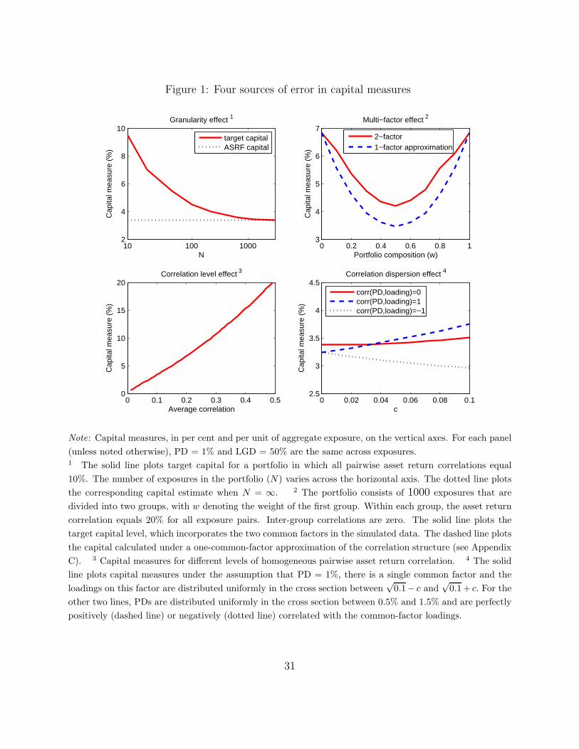
Figure 1: Four sources of error in capital measures
10 100 10002
4
6
8
10
N
Cap
ital m
easu
re (
%)
Granularity effect 1
target capitalASRF capital
0 0.2 0.4 0.6 0.8 13
4
5
6
7
Portfolio composition (w)
Cap
ital m
easu
re (
%)
Multi−factor effect 2
2−factor1−factor approximation
0 0.1 0.2 0.3 0.4 0.50
5
10
15
20
Average correlation
Cap
ital m
easu
re (
%)
Correlation level effect 3
0 0.02 0.04 0.06 0.08 0.12.5
3
3.5
4
4.5
c
Cap
ital m
easu
re (
%)
Correlation dispersion effect 4
corr(PD,loading)=0corr(PD,loading)=1corr(PD,loading)=−1
Note: Capital measures, in per cent and per unit of aggregate exposure, on the vertical axes. For each panel
(unless noted otherwise), PD = 1% and LGD = 50% are the same across exposures.1 The solid line plots target capital for a portfolio in which all pairwise asset return correlations equal
10%. The number of exposures in the portfolio (N) varies across the horizontal axis. The dotted line plots
the corresponding capital estimate when N = ∞. 2 The portfolio consists of 1000 exposures that are
divided into two groups, with w denoting the weight of the first group. Within each group, the asset return
correlation equals 20% for all exposure pairs. Inter-group correlations are zero. The solid line plots the
target capital level, which incorporates the two common factors in the simulated data. The dashed line plots
the capital calculated under a one-common-factor approximation of the correlation structure (see Appendix
C). 3 Capital measures for different levels of homogeneous pairwise asset return correlation. 4 The solid
line plots capital measures under the assumption that PD = 1%, there is a single common factor and the
loadings on this factor are distributed uniformly in the cross section between√
0.1− c and√
0.1 + c. For the
other two lines, PDs are distributed uniformly in the cross section between 0.5% and 1.5% and are perfectly
positively (dashed line) or negatively (dotted line) correlated with the common-factor loadings.
31
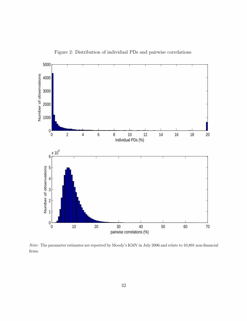
Figure 2: Distribution of individual PDs and pairwise correlations
0 2 4 6 8 10 12 14 16 18 200
1000
2000
3000
4000
5000
Individual PDs (%)
Nu
mb
er
of
ob
se
rva
tio
ns
0 10 20 30 40 50 60 700
1
2
3
4
5
6x 10
6
pairwise correlations (%)
Nu
mb
er
of
ob
se
rva
tio
ns
Note: The parameter estimates are reported by Moody’s KMV in July 2006 and relate to 10,891 non-financial
firms.
32
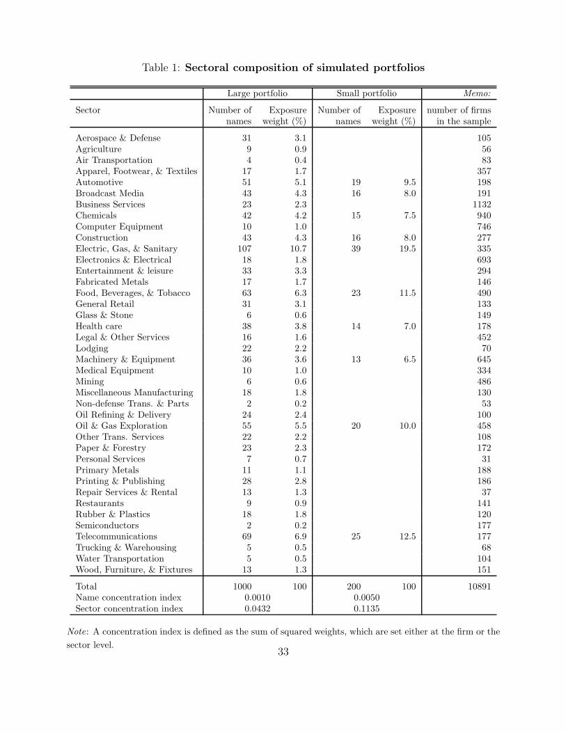
Table 1: Sectoral composition of simulated portfolios
Large portfolio Small portfolio Memo:
Sector Number of Exposure Number of Exposure number of firmsnames weight (%) names weight (%) in the sample
Aerospace & Defense 31 3.1 105Agriculture 9 0.9 56Air Transportation 4 0.4 83Apparel, Footwear, & Textiles 17 1.7 357Automotive 51 5.1 19 9.5 198Broadcast Media 43 4.3 16 8.0 191Business Services 23 2.3 1132Chemicals 42 4.2 15 7.5 940Computer Equipment 10 1.0 746Construction 43 4.3 16 8.0 277Electric, Gas, & Sanitary 107 10.7 39 19.5 335Electronics & Electrical 18 1.8 693Entertainment & leisure 33 3.3 294Fabricated Metals 17 1.7 146Food, Beverages, & Tobacco 63 6.3 23 11.5 490General Retail 31 3.1 133Glass & Stone 6 0.6 149Health care 38 3.8 14 7.0 178Legal & Other Services 16 1.6 452Lodging 22 2.2 70Machinery & Equipment 36 3.6 13 6.5 645Medical Equipment 10 1.0 334Mining 6 0.6 486Miscellaneous Manufacturing 18 1.8 130Non-defense Trans. & Parts 2 0.2 53Oil Refining & Delivery 24 2.4 100Oil & Gas Exploration 55 5.5 20 10.0 458Other Trans. Services 22 2.2 108Paper & Forestry 23 2.3 172Personal Services 7 0.7 31Primary Metals 11 1.1 188Printing & Publishing 28 2.8 186Repair Services & Rental 13 1.3 37Restaurants 9 0.9 141Rubber & Plastics 18 1.8 120Semiconductors 2 0.2 177Telecommunications 69 6.9 25 12.5 177Trucking & Warehousing 5 0.5 68Water Transportation 5 0.5 104Wood, Furniture, & Fixtures 13 1.3 151
Total 1000 100 200 100 10891Name concentration index 0.0010 0.0050Sector concentration index 0.0432 0.1135
Note: A concentration index is defined as the sum of squared weights, which are set either at the firm or the
sector level.33
Table 2: Summary statistics (in percent)
mean std. dev. skewness median minimum maximum
1-year PDs 2.67 5.28 2.49 0.39 0.02 20.00Pairwise correlations 9.24 3.86 1.87 8.45 0.29 65.00
Note: The sample includes 10,891 non-financial firms.
Table 3: Characteristics of simulated loan portfolios (in percent)
A. Large portfolios (1000 firms)mean std. dev. median minimum maximum
average PD 2.42 0.19 2.42 1.79 3.12std. dev. of individual PDs 5.16 0.26 5.16 4.25 6.14median PD 0.26 0.03 0.26 0.18 0.36average correlation 9.78 0.22 9.77 9.14 10.73std. dev. of loadings 9.33 0.31 9.32 8.33 10.47corr (PD, loadings) -20.0 2.04 -20.1 -26.7 -12.8
B. Small portfolios (200 firms)mean std. dev. median minimum maximum
average PD 2.28 0.36 2.26 1.24 3.68std. dev. of individual PDs 5.05 0.53 5.06 3.01 6.89median PD 0.24 0.05 0.23 0.11 0.55average correlation 10.49 0.44 10.48 8.99 12.00std. dev. of loadings 10.54 0.70 10.55 7.80 12.79corr (PD, loadings) -19.8 4.59 -20.2 -31.8 -1.2
Note: The results are based on 3,000 simulated portfolios and are carried out in two steps. First, portfolio-
specific characteristics specified by row headings are calculated for each simulated portfolio. Second, sum-
mary statistics specified by column headings are calculated for each of the portfolio specific characteristics
obtained in the first step. “Loadings” are estimated under a one-common-factor approximation of the cor-
relation structure and refer to the firm-specific loadings of asset returns on the single common factor.
34
Table 4: Capital measures and four sources of errors (in percent)
A. Large portfolios (1000 firms)
mean std. dev. median 95% interval 50% intervalTarget capital 1 3.31 0.18 3.30 [2.97, 3.67] [3.19, 3.42]
Deviation from target due to: 2
Multi-factor effect 3 -0.03 0.02 -0.03 [-0.08, 0.01] [-0.05, -0.02]Granularity effect 4 -0.16 0.004 -0.15 [-0.16, -0.15] [-0.16, -0.15]Correlation dispersion effect 5 0.39 0.05 0.39 [0.30, 0.48] [0.36, 0.42]Correlation level effect 6 0.61 0.06 0.62 [0.49, 0.73] [0.57, 0.66]
Shortcut capital (corr=12%) 4.12 0.20 4.12 [3.75, 4.51] [3.99, 4.25]
Memo: correlation level effect if:
corr=6% -1.06 0.08 -1.06 [-1.23, -0.92] [-1.11, -1.01]corr=18% 2.24 0.10 2.24 [2.05, 2.43] [2.17, 2.30]corr=24% 3.86 0.14 3.86 [3.59, 4.14] [3.77, 3.95]
B. Small portfolios (200 firms)
mean std. dev. median 95% interval 50% intervalTarget capital 1 3.86 0.32 3.85 [3.25, 4.55] [3.64, 4.07]
Deviation from target due to: 2
Multi-factor effect 3 -0.04 0.04 -0.04 [-0.12, 0.04] [-0.07, -0.01]Granularity effect 4 -0.73 0.03 -0.73 [-0.79, -0.67] [-0.75, -0.71]Correlation dispersion effect 5 0.42 0.12 0.42 [0.19, 0.65] [0.34, 0.50]Correlation level effect 6 0.40 0.13 0.40 [0.16, 0.67] [0.32, 0.48]
Shortcut capital (corr=12%) 3.91 0.38 3.90 [3.17, 4.70] [3.64, 4.16]
Memo: correlation level effect if:
corr=6% -1.19 0.13 -1.19 [-1.46, -0.95] [-1.28, -1.10]corr=18% 1.95 0.21 1.94 [1.57, 2.38] [1.81, 2.08]corr=24% 3.50 0.30 3.49 [2.94, 4.12] [3.30, 3.70]
Note: Summary statistics for the simulated portfolios underpinning Table 3. The column entitled “95%
interval” reports the 2.5th and 97.5th percentiles of the statistics specified in the particular row heading.
The column entitled “50% interval” reports the corresponding 25th and 75th percentiles. In all calculations,
LGDi follows a symmetric triangular distribution between 0 and 1.1 Based on Moody’s KMV estimates of PDs and asset return correlations and a Monte Carlo procedure for
calculating the probability distribution of default losses. 2 Four sources of deviation from the target capital
level; a negative sign implies underestimation. The sum of the target capital level and the four deviations
equals the shortcut capital level. Each deviation is based on the assumptions underlying previous deviations
plus one additional assumption. 3 For the multi-factor effect, the correlation matrix underpinning the
target capital level is approximated under the assumption that there is a single common factor. 4 For
the granularity effect, there is the additional assumption that the number of firms is infinite. 5 For the
correlation dispersion effect, the additional assumption is that the loadings on the single common factor are
the same across exposures. 6 For the correlation level effect, the additional assumption imposes a different,
shortcut, level on the constant pairwise correlation.
35
Table 5: Explaining calibration-driven capital discrepancies
Regression 1 Regression 2
Large Small Pooled Large Small Pooledportfolio portfolio sample portfolio portfolio sample
constant 3.01 3.00 3.29 2.58 2.40 2.46(65.6) (53.0) (111.6) (129.6) (84.0) (159.8)
average corr -0.24 -0.23 -0.24 -0.28 -0.26 -0.27(34.8) (31.5) (48.8) (95.6) (74.4) (114.5)
std dev of loading coefficients 0.037 0.022 0.010 0.031 0.029 0.028(7.5) (4.8) (3.1) (14.6) (13.9) (19.9)
average PD 0.21 0.19 0.19(86.2) (61.6) (94.2)
corr(PD, loading coefficient) -0.018 -0.019 -0.019(80.5) (79.5) (113.9)
adjusted R2 0.39 0.33 0.56 0.89 0.86 0.91
Note: t-statistics in parentheses. The regression is based on 3,000 simulations for each portfolio size. The
dependent variable equals shortcut capital (based on asset return correlation of 12%) minus target capital,
net of the granularity and multi-factor effects (see Table 4). Loading coefficients are estimated under a
one-common-factor approximation of the correlation structure of asset returns. The last regressor equals the
Kendall rank correlation between PDs and loading coefficients.
36

Table 6: Impact of estimation errors (in per cent)
A. Sample average of pairwise correlationsN=100 N=200 N=500 N=1000
T=60 9.72 [6.5, 13.3] 9.67 [6.4, 13.3] 9.64 [6.6, 13.0] 9.63 [6.9, 12.7]T=120 9.77 [7.4, 12.4] 9.77 [7.6, 12.1] 9.76 [7.6, 12.1] 9.72 [7.7, 12.0]T=300 9.75 [8.3, 11.3] 9.79 [8.3, 11.3] 9.74 [8.4, 11.2] 9.77 [8.4, 11.25]
B. Sample standard deviation of loading coefficientsN=100 N=200 N=500 N=1000
T=60 12.11 [10.3, 14.1] 11.84 [10.5, 13.2] 11.65 [10.8, 12.5] 11.58 [10.8, 12.2]T=120 8.50 [7.4, 9.8] 8.34 [7.5, 9.1] 8.17 [7.6, 8.8] 8.13 [7.7, 8.6]T=300 5.35 [4.6, 6.2] 5.24 [4.7, 5.7] 5.16 [4.8, 5.5] 5.12 [4.9, 5.4]
C. Estimated capital, based on one-factor loading structureN=100 N=200 N=500 N=1000
T=60 3.87 [2.8, 5.1] 3.83 [2.8, 5.0] 3.80 [2.8, 4.9] 3.79 [2.9, 4.8]T=120 3.59 [2.9, 4.4] 3.58 [2.9, 4.4] 3.56 [2.9, 4.3] 3.54 [2.9, 4.3]T=300 3.41 [3.0, 3.9] 3.42 [3.0, 3.9] 3.40 [3.0, 3.9] 3.41 [3.0, 3.9]benchmark 3.31 3.31 3.31 3.31
Note: Results are based on 1000 simulations of the asset returns of N firms over T months, with the true
pairwise correlation, PD and LGD fixed at 9.78%, 1% and 50%, respectively. Each cell contains the mean
and the 95% confidence interval of: the average of sample pairwise correlations (panel A); the standard
deviation of the loading coefficients in a one-factor approximation (panel B); and the implied capital buffer
(panel C).
37
Table 7: Alternative distributional assumptions
Degrees of Capital measure2 Mean kurtosis3 Median kurtosis3
freedom1 (in per cent) mean 95% interval mean 95% interval
(3, 3) 6.17 7.83 [7.30, 8.27] 5.54 [5.11, 6.54](4, 4) 4.59 5.72 [5.47, 5.92] 4.43 [4.25, 4.59](5, 5) 4.03 4.79 [4.64, 4.93] 3.96 [3.85, 4.06](6, 6) 3.81 4.31 [4.19, 4.40] 3.70 [3.63, 3.78](7, 7) 3.67 4.02 [3.93, 4.10] 3.55 [3.49, 3.60](8, 8) 3.59 3.83 [3.76, 3.89] 3.44 [3.39, 3.49](9, 9) 3.53 3.70 [3.64, 3.75] 3.36 [3.32, 3.40](10, 10) 3.49 3.60 [3.55, 3.65] 3.30 [3.26, 3.34](∞, ∞) 3.31 3.00 [2.99, 3.01] 2.89 [2.88, 2.90]
1 The degrees of freedom of the Student-t distribution of asset returns’ common and idiosyncratic factors,
respectively. The last row refers to a Gaussian specification. 2 Obtained by applying the general ASRF
formula (equation 4) to a homogeneous portfolio, in which PD=1% and LGD=50% for each exposure and
asset return correlations equal 9.78% for each pair of exposures. The default boundary for such exposures
is calculated on the basis of 10 million simulations. 3 The means and the 95% confidence intervals (based
on 10,000 Monte Carlo simulations) of the estimators of the cross-sectional mean and median of the kurtosis
when: (i) the marginal Student-t distributions of the common and idiosyncratic factors have the degrees
of freedom specified in the row heading and asset return correlations equal 9.78%; (ii) the available data
comprise time series of 59 returns for 10,891 firms.
38